Ro-vibrational energy analysis of Manning-Rosen and Pöschl-Teller potentials with a new improved approximation in the centrifugal term

Abstract

Two physically important potentials (Manning-Rosen and Pöschl-Teller) are considered for the ro-vibrational energy in diatomic molecules. An improved new approximation is invoked for the centrifugal term, which is then used for their solution within the Nikiforov-Uvarov framework. This employs a recently proposed scheme, which combines the two widely used Greene-Aldrich and Pekeris-type approximations. Thus, approximate analytical expressions are derived for eigenvalues and eigenfunctions. The energies are examined with respect to two approximation parameters, $\lambda$ and $\nu$. The original approximations are recovered for certain specials values of these two parameters. This offers a simple effective scheme for these and other relevant potentials in quantum mechanics.

background-colorgray0.98

1 Introduction

The construction of a general, universal potential energy function for molecules has been at the forefront of research activity in chemical, molecular and solid-state physics, as it carries the relevant information for a given molecule. They are needed as input in various areas including spectroscopy, molecule-molecule collision, molecular simulation, dynamical situation, thermodynamic properties etc. There are non-trivial challenges faced towards the development of energy-distance relationship, due to which, its general form still remains elusive. The publication of famous exponential Morse potential about 90 years ago, has inspired a broad range of works along this direction having varying degrees of sophistication, accuracy and flexibility. A vast number of such functions have been generated over the years by a number of researchers. Generally speaking, as the number of parameters in the analytic potential function increases, the greater it fits with the experimental data.

The exponential Manning-Rosen (MR) potential [1],

$$V=V_{MR}(r)=\frac{\hbar^{2}}{2\mu b^{2}}\left[\frac{\alpha(\alpha-1)e^{-2r/b}}{(1-e^{-r/b})^{2}}-\frac{Ae^{-r/b}}{1-e^{-r/b}}\right],$$ (1)

has played the role of an important mathematical model in the context of molecular vibration and rotation. It has relevance to a multitude of bound and resonance-state problems in physics. This expression contains two dimensionless parameters $A$ (signifying the strength) and $\alpha$ (constant), whereas the screening parameter $b$ (having a dimension of length) is connected to the range of potential. Some interesting properties include (i) it is invariant under transformation $\alpha\leftrightarrow\alpha-1$ (ii) this reduces to the celebrated short-range Hulthén potential for $\alpha=0$ or 1 (iii) a relative minimum occurs for $r=b\ln\left[1+\frac{2\alpha(\alpha-1)}{A}\right]$, when $\alpha>1$ and $A>0$.

The Schrödinger equation for the so-called $s$ (non-zero $\ell$) states can be obtained exactly, by a number of elegant and attractive formalisms, such as direct factorization method, Feynman path-integral formalism, standard function analysis leading to wave functions expressed in terms of hyper-geometric functions, a tridiagonal matrix representation [2, 3, 4], etc. However, the same for $\ell\neq 0$ states are yet to be found in closed analytic form, giving rise to a number of notable approximate schemes. Thus, arbitrary $\ell$ states were calculated by means of an approximation of centrifugal term: $\frac{1}{r^{2}}\approx\frac{1}{b^{2}}\frac{e^{-r/b}}{(1-e^{-r/b})^{2}}$ in short range [5], similar along the lines of familiar Pekeris scheme. In the literature, other methods are also available, such as, a super-symmetric shape invariance formalism along with a function analysis [6], $1/r^{2}$ approximated by a term having 3 adjustable parameters [7], Nikiforov-Uvarov (NU) method with an approximation of the $1/r^{2}$ term [8], path-integral formalism approached by a Duru-Kleinert method [9]. In [10], the author used Laguerre and oscillator bases for tridiagonalization of relevant Hamiltonian and a Gauss quadrature to calculate potential matrix elements. Other significant works are: J-matrix method [11] with a proper expansion for $1/r^{2}$, numerical integrating procedure in MATHEMATICA [12], generalized pseudospectral method [13], etc. While most works focused on bound states, scattering states [4, 11] were also considered. Moreover, properties such as oscillator strengths, multipole moments, transition probabilities for certain states were reported in the literature [11]. It has been probed in higher dimension [14].

Another important diatomic molecular potential is the Pöschl-Teller (PT) [15] like model, given by,

$$V=V_{PT}(r)=\frac{\xi_{1}-\xi_{2}\cosh(\alpha r)}{\sinh^{2}(\alpha r)},$$ (2)

where $r$ denotes the internuclear distance, $\xi_{1},\xi_{2}$ are two parameters controlling the potential well, and $\alpha$ governs the range of potential. Its bound states for arbitrary quantum numbers were expressed in terms of hyper-geometric functions ${}_{2}F_{1}(a,b,c;z)$, by employing an approximation to $1/r^{2}$ [16]. One of its variants, the so-called Scarf potential was analyzed by expanding the $1/r^{2}$ term around the minimum equilibrium point [17]. A comparison of Pekeris- as well as Greene-Aldrich-like approximations for the centrifugal term, in the context of ro-vibrational states, have been presented lately [18, 19]. The scattering states have found discussion [20, 21] as well.

Thus it appears that there is a preponderance of approaches which involve a well-designed approximation for the centrifugal term. Broadly speaking, two major routes have gained popularity over the years, namely the Pekeris- [22, 23, 24, 25] and Greene-Aldrich-type approximations, along with their several variations [26]. The primary objective of this work is to present an extension/modification of such schemes for the two potentials mentioned in Eqs. 1 and 2. The new proposed scheme has been recently applied successfully for energy and thermodynamic analysis of Deng-Fan molecular potential [27]. Towards this end, we will express the centrifugal term as a linear combination of two approximations which turns out (from the future discussion) to offer an accurate alternative approximation to the centrifugal term, near the origin ($r=0$) and any other point ($r=r_{0}$). This new intuitive approximation is succinctly discussed as functions of $r$, $r_{0}$ and two approximating parameters, namely, $\lambda$, $\nu$. The corresponding energy spectra generated from our current approximation are then critically compared with the available established approximations for the centrifugal term, for some representative states. This is done for both MR and PT potentials.

The article is organized as follows. Section 2, at first, provides the formal solutions of Schrödinger equation within the NU method. The eigenvalues and eigenfunctions for MR and PT within the various approximations of centrifugal term, are derived in Secs. 3 and 4 respectively. The associated energy spectra are analyzed in Sec. 5. Moreover, the effect of the approximation parameters $\lambda$ and $\nu$ on the energy spectrum of MR and PT potentials are shown in Finally a few comments are made in Sec. 6.

2 Exact solution of the Schrödinger equation by Nikiforov-Uvarov Method

Let us consider the Schrödinger equation of a diatomic molecule,

$$-\frac{\hbar^{2}}{2\mu}\nabla^{2}\psi+V({\bf r})\psi=E\psi,$$ (3)

in presence of MR ($V({\bf r})=V_{MR}(r))$ or PT ($V({\bf r})=V_{PT}(r))$ potential of Eq. (1) and Eq. (2) respectively. Here,

$$\nabla^{2}=\frac{1}{r^{2}}\frac{\partial}{\partial r}\left(r^{2}\frac{\partial}{\partial r}\right)+\frac{1}{r^{2}\sin\theta}\frac{\partial}{\partial\theta}\left(\sin\theta\frac{\partial}{\partial\theta}\right)+\frac{1}{r^{2}\sin^{2}\theta}\frac{\partial^{2}}{\partial\phi^{2}},$$ (4)

and $\mu$ is the reduced mass of a diatomic molecule, $r$ is the internuclear distance. The MR potential, $V_{MR}$ has a minimum at $r=b\ln\left[1+\frac{2\alpha(\alpha-1)}{A}\right]$, whereas the same occurs at $r=\frac{1}{\alpha}\tanh^{-1}\left(\sqrt{\frac{2a}{b}}\right)$ in case of $V_{PT}$. Let

$$\psi({\bf r})=\frac{R(r)}{r}Y_{l}^{m}(\theta)\,e^{im\phi},$$ (5)

be the solution of Eq. (3). Then one obtains,

$$\frac{d^{2}R}{dr^{2}}+\left[\frac{2\mu}{\hbar^{2}}E-\frac{2\mu}{\hbar^{2}}V(r)-\frac{l(l+1)}{r^{2}}\right]R=0,$$ (6)

and

$$Y_{l}^{m}=\left[\frac{(2l+1)(l-|m|)!}{4\pi(l+|m|)!}\right]^{\frac{1}{2}}\,P_{l}^{|m|}(\cos\theta)\,e^{im\phi},$$ (7)

where $l(l+1)$ is the separation constant. To find the general solution of resulting radial Schrödinger equation obtained in Eq. (6), we will use a transformation $s=e^{-r/b}$ for MR and $s=\tanh^{2}(\alpha r/2)$ for PT potentials respectively. Moreover, we have considered two set of bases, viz., (i) $\left\{1,\frac{e^{-r/b}}{1-e^{-r/b}},\frac{e^{-2r/b}}{(1-e^{-r/b})^{2}}\right\}$, for MR and (ii) $\left\{1,\frac{1}{\sinh^{2}\alpha r},\frac{\cosh\alpha r}{\sinh^{2}\alpha r}\right\}$, for PT potential, for which the centrifugal term is approximated in different forms, such as Greene-Aldrich [26] and Pekeris-type [22]. Then the Schrödinger equation becomes a second-order differential equation of the form given below,

$$\frac{d^{2}R}{ds^{2}}+\frac{\widetilde{\tau}(s)}{\sigma(s)}\frac{dR}{ds}+\frac{\widetilde{\sigma}(s)}{\sigma^{2}(s)}R=0,$$ (8)

where $\widetilde{\tau}(s)$, $\sigma(s)$, $\widetilde{\sigma}(s)$ are polynomials in $s$ of degree one, two and two respectively. If we let,

$$R(s)=\phi_{1}(s)\phi_{2}(s),$$ (9)

be the solution of Eq. (8), then we obtain [28],

$$\sigma(s)\phi_{2}^{{}^{\prime\prime}}(s)+\tau(s)\phi^{\prime}_{2}(s)+\nu\,\phi_{2}(s)=0,$$ (10)

and

$$\begin{array}[]{l}\phi_{1}(s)=\displaystyle e^{\int\frac{\pi(s)}{\sigma(s)}ds},\end{array}$$ (11)

where

$$\begin{array}[]{ll}\pi(s)&=\frac{\sigma^{\prime}(s)-\widetilde{\tau}(s)}{2}\pm\sqrt{\left(\frac{\sigma^{\prime}(s)-\widetilde{\tau}(s)}{2}\right)^{2}-\widetilde{\sigma}(s)+k\,\sigma(s)},\\ \tau(s)&=\widetilde{\tau}(s)+2\pi(s),~{}\bar{\nu}=k+\pi^{\prime}(s),\end{array}$$ (12)

$\bar{\nu}$ and $k$ are real constants. Since $\pi(s)$ is a polynomial in $s$, we have to find $k$ in such a way that, $\left(\frac{\sigma^{\prime}(s)-\widetilde{\tau}(s)}{2}\right)^{2}-\widetilde{\sigma}(s)+k\,\sigma(s)$ is a square of a polynomial in $s$. Then the solutions of Eq. (10) are given by,

$$\phi_{2,n_{r}}(s)=\frac{1}{\rho(s)}\frac{d^{n_{r}}}{ds^{n_{r}}}\left[\sigma^{n_{r}}(s)\rho(s)\right],$$ (13)

and eigenvalues are obtained as,

$$\nu_{n_{r}}=-{n_{r}}\,\tau^{\prime}(s)-\frac{{n_{r}}({n_{r}}-1)}{2}\sigma^{{}^{\prime\prime}}(s),~{}{n_{r}}=0,1,2,\dots,$$ (14)

where

$$\begin{array}[]{l}\rho(s)=\displaystyle\left[\sigma(s)\right]^{-1}\,e^{\int\frac{\tau(s)}{\sigma(s)}ds}.\end{array}$$ (15)

3 NU method for MR potential

3.1 Approximation 1: Greene-Aldrich-type

Following [5, 6, 8, 26, 29, 30, 31, 32, 33, 34, 35], at first, let us consider,

$$\begin{array}[]{ll}\frac{1}{r^{2}}&\approx f_{1}(r)=\frac{1}{b^{2}}\left(x_{11}+\frac{x_{21}e^{-r/b}}{1-e^{-r/b}}+\frac{x_{31}e^{-2r/b}}{(1-e^{-r/b})^{2}}\right),\end{array}$$ (16)

where

$$x_{11}=\frac{1}{12},x_{21}=1,x_{31}=1,$$ (17)

when $r/b\ll 1$. In the limiting case, $\lim\limits_{b\rightarrow\infty}\frac{1}{b^{2}}\left(\frac{1}{12}+\frac{s}{1-s}+\frac{s^{2}}{(1-s)^{2}}\right)=\frac{1}{r^{2}}$. Therefore, for a fixed $b$, Eq. (16) is a good approximation near $r=0$. It is to be mentioned that, for $x_{11}=0,x_{21}=x_{31}=1$, this approximation corresponds to that of [5, 29], whereas for $x_{11}=0,x_{21}=e^{1/b},x_{31}=1$, it refers to [31, 32].

3.2 Approximation 2: Pekeris-type

In another attempt, $\frac{1}{r^{2}}$ can be expressed [22, 7] around $r=r_{0}$, as,

$$\frac{1}{r^{2}}\approx f_{2}(r)=\frac{1}{b^{2}}\left(x_{12}+\frac{x_{22}e^{-r/b}}{1-e^{-r/b}}+\frac{x_{32}e^{-2r/b}}{(1-e^{-r/b})^{2}}\right),$$ (18)

where

$$\begin{array}[]{ll}x_{12}&=\displaystyle\frac{3-3u+u^{2}+\left(2u-6\right)s_{0}+\left(u+3\right)s_{0}^{2}}{u^{4}},\\ x_{22}&=\displaystyle\frac{2\left(1-s_{0}\right)^{2}}{u^{4}}\left(3+u+\frac{2u-3}{s_{0}}\right),\\ x_{32}&=-\displaystyle\frac{\left(1-s_{0}\right)^{3}}{u^{4}}\left(\frac{3+u}{s_{0}}+\frac{u-3}{s_{0}^{2}}\right),\\ s_{0}&=e^{-u},~{}u=\frac{r_{0}}{b}.\end{array}$$ (19)

In particular, if $r_{0}=b\ln\left[1+\frac{2\alpha(\alpha-1)}{A}\right]$, then the potential value $V_{MR}(r_{0})$ is minimum, which is equal to $-\frac{A^{2}\hbar^{2}}{8\mu b^{2}\alpha(\alpha-1)}$ for $A>0$ and $\alpha\in(-\infty,0)\cup(1,\infty)$.

3.3 Approximation 3: Pekeris-type

In [36, 8], the authors considered an approximation of the following form,

$$\frac{1}{r^{2}}\approx f_{3}(r)=\frac{1}{b^{2}}\left(x_{13}+\frac{x_{23}e^{-r/b}}{1-e^{-r/b}}+\frac{x_{33}e^{-2r/b}}{\left(1-e^{-r/b}\right)^{2}}\right),$$ (20)

where

$$\begin{array}[]{ll}x_{13}&=\frac{12\epsilon_{1}^{2}-4\epsilon_{1}(2A+3\epsilon_{1})\log(\epsilon_{2})+\epsilon_{3}^{2}\log(\epsilon_{2})^{2}}{\epsilon_{4}^{2}\log(\epsilon_{2})^{4}},\\ x_{23}&=\frac{8\epsilon_{1}^{2}\left[-6\epsilon_{1}+(3A+4\epsilon_{1})\log(\epsilon_{2})\right]}{A\epsilon_{4}^{2}\log(\epsilon_{2})^{4}},\\ x_{33}&=-\frac{16\epsilon_{1}^{3}\left[-3\epsilon_{1}+\epsilon_{3}\log(\epsilon_{2})\right]}{A^{2}\epsilon_{4}^{2}\log(\epsilon_{2})^{4}},\\ \epsilon_{1}&=\alpha(\alpha-1),~{}\epsilon_{2}=1+\frac{2\alpha(\alpha-1)}{A},\\ \epsilon_{3}&=A\epsilon_{2},~{}\epsilon_{4}=b\epsilon_{3}.\end{array}$$ (21)

3.4 Approximation 4: A linear combination of Greene-Aldrich and Pekeris-type

Now, we propose a new approximation of the form [27],

$$\frac{1}{r^{2}}\approx f_{4}(r,\lambda,\nu)=\frac{1}{b^{2}}\left(x_{1}+\frac{x_{2}e^{-r/b}}{1-e^{-r/b}}+\frac{x_{3}e^{-2r/b}}{(1-e^{-r/b})^{2}}\right),$$ (22)

where

$$\begin{array}[]{l}\left(\begin{array}[]{l}x_{1}\\ x_{2}\\ x_{3}\end{array}\right)=\left(\begin{array}[]{lll}x_{11}&x_{12}&x_{13}\\ x_{21}&x_{22}&x_{23}\\ x_{31}&x_{32}&x_{33}\end{array}\right)\left(\begin{array}[]{l}\nu\lambda\\ \nu(1-\lambda)\\ 1-\nu\end{array}\right),\end{array}$$ (23)

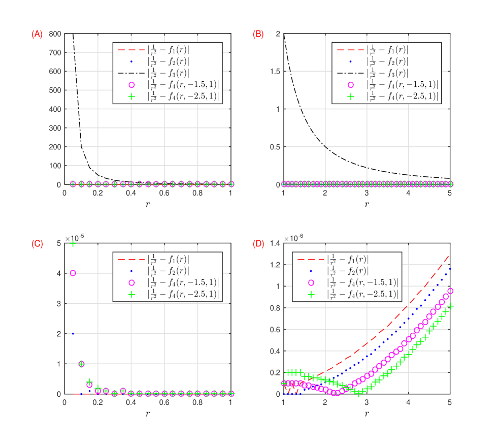
Figure 1: Plot of the differences between exact centrifugal term $\frac{l(l+1)}{r^{2}}$ and various approximations from Eqs. (16), (18), (20), (22) in MR potential, for $l=1,\hbar=\mu=1,\alpha=1.5,b=1/0.05,A=2b$, in panels (A)-(D) respectively.

and $\lambda,\nu$ are dimensionless real constants. In Fig. 1, the centrifugal term under different approximations defined in Eqs. (16), (18), (20) and (22), is displayed. From this figure, it is clear that, Eq. (22) gives the best approximation amongst all. If $(\lambda,\nu)=(1,1)$, then Eq. (22) implies Eq. (16); if $(\lambda,\nu)=(0,1)$, then it leads to Eq. (18); if $(\lambda,\nu)=(\lambda,0)$, then it implies Eq. (20). The approximation is suitable for negative values of $\lambda$ for large $r$. Furthermore, it is applicable for any values of $r$.

3.5 Solution of the MR potential

Now, under the transformation, $s=e^{-r/b}$, Eq.(6) becomes,

$$\begin{array}[]{l}\frac{d^{2}R}{ds^{2}}+\frac{1-s}{s(1-s)}\frac{dR}{ds}+\frac{-A_{1}s^{2}+Bs-C}{s^{2}(1-s)^{2}}R=0,\end{array}$$ (24)

where

$$\begin{array}[]{ll}A_{1}&=\bar{\varepsilon}^{2}+A+\alpha(\alpha-1)+l(l+1)(x_{3}-x_{2}),\\ B&=2\bar{\varepsilon}^{2}+A-l(l+1)x_{2},\\ C&=\bar{\varepsilon}^{2}=l(l+1)x_{1}-\varepsilon,\varepsilon=\frac{2\mu b^{2}E}{\hbar^{2}}.\end{array}$$ (25)

According to NU method, we obtain a pair of $k$, as given by [37],

$$\begin{array}[]{ll}k_{\pm}=A-l(l+1)x_{2}\pm\bar{\varepsilon}\sqrt{(2\alpha-1)^{2}+4l(l+1)x_{3}}.\end{array}$$ (26)

Applying Eq. (26) in Eq. (12), we obtain,

$$\begin{array}[]{ll}\pi(s)&=-\frac{s}{2}\pm\left\{\begin{array}[]{lll}\left(\bar{\varepsilon}-\frac{1}{2}\sqrt{(2\alpha-1)^{2}+4l(l+1)x_{3}}\right)s+\bar{\varepsilon},&k=k_{+},&k_{+}-B>0\\ \left(\bar{\varepsilon}+\frac{1}{2}\sqrt{(2\alpha-1)^{2}+4l(l+1)x_{3}}\right)s+\bar{\varepsilon},&k=k_{-},&k_{-}-B>0\\ \left(\bar{\varepsilon}-\frac{1}{2}\sqrt{(2\alpha-1)^{2}+4l(l+1)x_{3}}\right)s-\bar{\varepsilon},&k=k_{+},&k_{+}-B<0\\ \left(\bar{\varepsilon}+\frac{1}{2}\sqrt{(2\alpha-1)^{2}+4l(l+1)x_{3}}\right)s-\bar{\varepsilon},&k=k_{-},&k_{-}-B<0\end{array}\right\}.\end{array}$$ (27)

For the potential in Eq. (1), we have chosen $k=k_{-}$ with $k_{-}-B<0$, and selected,

$$\pi(s)=-\frac{s}{2}-\left(\bar{\varepsilon}+\frac{1}{2}\sqrt{(2\alpha-1)^{2}+4l(l+1)x_{3}}\right)s+\bar{\varepsilon}.$$ (28)

This gives,

$$\begin{array}[]{l}\rho(s)=s^{2\bar{\varepsilon}}(1-s)^{2L-1},\\ \phi_{1}(s)=s^{\bar{\varepsilon}}(1-s)^{L},\end{array}$$ (29)

and

$$\begin{array}[]{ll}\phi_{2,n_{r}}&=({n_{r}})!\,P_{n_{r}}^{(2\bar{\varepsilon},2L-1)}(1-2s),\\ &=\frac{\Gamma\left(n_{r}+2\bar{\varepsilon}+1\right)}{\Gamma\left(2\bar{\varepsilon}+1\right)}{}_{2}F_{1}\left(-n_{r},n_{r}+2\bar{\varepsilon}+2L;2\bar{\varepsilon}+1;s\right),\end{array}$$ (30)

where

$$L=\frac{1}{2}+\frac{1}{2}\sqrt{(2\alpha-1)^{2}+4l(l+1)x_{3}}.$$ (31)

The eigenvalues, $E_{n_{r},l}^{MR}$, will then be generated from the following relation,

$$k+(2n_{r}+1)\pi^{\prime}(s)=n_{r}^{2}.$$ (32)

Finally, we obtain the ro-vibrational energy spectrum of MR potential, as a function of $(\hbar,\mu),(\alpha,b),(\lambda,\nu)$, as given below,

$$\begin{array}[]{ll}E_{n_{r},l}^{MR}&=x_{5}-\frac{\hbar^{2}}{2\mu b^{2}}\left(\frac{x_{4}^{2}}{(n_{r}+L)^{2}}+\frac{(n_{r}+L)^{2}}{4}\right),\end{array}$$ (33)

where

$$\begin{array}[]{ll}x_{4}=\frac{1}{2}\left[A+\alpha(\alpha-1)+l(l+1)(x_{3}-x_{2})\right],x_{5}=\frac{\hbar^{2}}{2\mu b^{2}}(l(l+1)x_{1}+x_{4}).\end{array}$$ (34)

Therefore, the radial wave function of MR potential can be expressed as [38],

$$R_{n_{r}}^{MR}(r)=N_{{n_{r}},l}\,s^{\bar{\varepsilon}}(1-s)^{L}\,{}_{2}F_{1}\left(-{n_{r}},{n_{r}}+2\bar{\varepsilon}+2L;2\bar{\varepsilon}+1;s\right),$$ (35)

where

$$N_{{n_{r}},l}=\left[\frac{2\bar{\varepsilon}(n_{r}+\bar{\varepsilon}+L)\Gamma(n_{r}+2\bar{\varepsilon}+1)\Gamma(n_{r}+2\bar{\varepsilon}+2L)}{({n_{r}})!b(n_{r}+\bar{\varepsilon})\Gamma(n_{r}+2L)\left[\Gamma(2\bar{\varepsilon}+1)\right]^{2}}\right]^{\frac{1}{2}},$$ (36)

is the normalization constant, to be obtained from,

$$\int|\psi_{n_{r},l,m}^{MR}({\bf r})|^{2}\,d{\bf r}=1,~{}d{\bf r}=r^{2}\sin\theta\,dr\,d\theta\,d\phi.$$ (37)

Finally, the explicit form of eigenfunctions of MR potential can be written as,

$$\psi_{n_{r},l,m}^{MR}({\bf r})=\left[\frac{(2l+1)(l-|m|)!}{4\pi(l+|m|)!}\right]^{\frac{1}{2}}\frac{N_{{n_{r}},l}}{r}\,s^{\bar{\varepsilon}}(1-s)^{L}\,{}_{2}F_{1}\left(-{n_{r}},{n_{r}}+2\bar{\varepsilon}+2L;2\bar{\varepsilon}+1;s\right)\,P_{l}^{m}(\cos\theta)\,e^{im\phi},~{}s=e^{-r/b}.$$ (38)

It is to be noted that the approximation (22) is well defined for $\lambda,\nu$ satisfying,

$$\begin{array}[]{l}(2\alpha-1)^{2}+4l(l+1)\left(x_{31}\nu\lambda+x_{32}\nu(1-\lambda)+x_{33}(1-\nu)\right)>0,\\ x_{11}\nu\lambda+x_{12}\nu(1-\lambda)+x_{13}(1-\nu)>0.\end{array}$$ (39)

4 NU method for PT potential

4.1 Approximation 1: Greene-Aldrich type

At first, we consider an approximation [39] of the form,

$$\frac{1}{r^{2}}\approx f_{1}(r)=\alpha^{2}\left(x_{11}+\frac{x_{21}}{\sinh^{2}\alpha r}+\frac{x_{31}\cosh\alpha r}{\sinh^{2}\alpha r}\right),$$ (40)

where

$$x_{11}=0,x_{21}=\frac{1}{2},x_{31}=\frac{1}{2}.$$ (41)

4.2 Approximation 2: Greene-Aldrich type

Next let us examine another Greene-type approximation due to [26, 18],

$$\frac{1}{r^{2}}\approx f_{2}(r)=\alpha^{2}\left(x_{12}+\frac{x_{22}}{\sinh^{2}\alpha r}+\frac{x_{32}\cosh\alpha r}{\sinh^{2}\alpha r}\right),$$ (42)

where

$$x_{12}=\frac{1}{12},x_{22}=\frac{1}{2},x_{32}=\frac{1}{2}.$$ (43)

4.3 Approximation 3: Pekeris-type

The Pekeris-type approximation, around $r=r_{0}$ is given by [18, 22, 23, 20, 24, 25],

$$\frac{1}{r^{2}}\approx f_{3}(r)=\alpha^{2}\left(x_{13}+\frac{x_{23}}{\sinh^{2}\alpha r}+\frac{x_{33}\cosh\alpha r}{\sinh^{2}\alpha r}\right),$$ (44)

where

$$\begin{array}[]{ll}x_{13}=\displaystyle\frac{1}{u^{4}}\left(3+u^{2}-3u\coth u\right),\\ x_{23}=\displaystyle\frac{1}{4u^{4}}\left(18+6\cosh(2u)-23u\coth u-u\cosh(3u)\ \mathrm{cosech}\ u\right),\\ x_{33}=\displaystyle\frac{1}{u^{4}}\left(4u+2u\cosh(2u)-3\sinh(2u)\right)\ \mathrm{cosech}\ u,\\ u=\alpha r_{0}.\end{array}$$ (45)

In particular, if $r_{0}=\frac{1}{\alpha}\tanh^{-1}\left(\sqrt{\frac{2\sqrt{\xi_{1}^{2}-\xi_{2}^{2}}}{\xi_{1}+\sqrt{\xi_{1}^{2}-\xi_{2}^{2}}}}\right)$, then the potential has a minimum at $r=r_{0}$.

4.4 Approximation 4: A linear combination of Greene-Aldrich and Pekeris-type

Now let us discuss a linear combination of three approximations in Eqs. (40), (42), (44), proposed lately [27],

$$\frac{1}{r^{2}}\approx f_{4}(r,\lambda,\nu)=\alpha^{2}\left(x_{1}+\frac{x_{2}}{\sinh^{2}\alpha r}+\frac{x_{3}\cosh\alpha r}{\sinh^{2}\alpha r}\right),$$ (46)

where

$$\left(\begin{array}[]{c}x_{1}\\ x_{2}\\ x_{3}\end{array}\right)=\left(\begin{array}[]{ccc}x_{11}&x_{12}&x_{13}\\ x_{21}&x_{22}&x_{23}\\ x_{31}&x_{32}&x_{33}\end{array}\right)\left(\begin{array}[]{l}\nu\lambda\\ \nu(1-\lambda)\\ 1-\nu\end{array}\right),$$ (47)

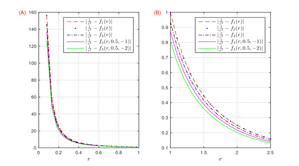
Figure 2: Plot of the differences between exact centrifugal term $\frac{l(l+1)}{r^{2}}$ and various approximations from Eqs. (40), (42), (44) and (46) in PT potential, for $l=1,\hbar=\mu=1,\xi_{1}=4,\xi_{2}=2,\alpha=0.05$, in panels (A)-(D) respectively.

and $\lambda,\nu$ are real constants. In Fig. 2, the centrifugal term under different approximations, defined in Eqs. (40), (42), (44) and (46) are displayed. It is quite clear that, the approximation of Eq. (46) is the best of all. When $(\lambda,\nu)=(1,1)$, Eq. (46) implies Eq. (40); $(\lambda,\nu)=(0,1)$ means (42); $(\lambda,\nu)=(\lambda,0)$, leads to (44). It may be noted that, Eq. (46) is good for negative $\nu$ in the large-$r$ region. The advantage is that, for any arbitrary values of $r$, this approximation is easily seen to provide the best representation amongst all, for select values of $\lambda$ and $\nu$.

4.5 Solution of the PT potential

Under the transformation, $s=\tanh^{2}\frac{\alpha r}{2}$, the radial Schrödinger equation in (6) becomes,

$$\begin{array}[]{l}\frac{d^{2}R}{ds^{2}}+\frac{1-3s}{s(1-s)}\frac{dR}{ds}+\frac{-As^{2}+Bs-C}{s^{2}(1-s)^{2}}R=0,\end{array}$$ (48)

where

$$\begin{array}[]{ll}A&=\frac{\mu}{2\alpha^{2}\hbar^{2}}(\xi_{1}+\xi_{2})+\frac{l(l+1)}{4}(x_{3}-x_{2}),\\ B&=\frac{2\mu}{\alpha^{2}\hbar^{2}}\left(E+\frac{\xi_{1}}{2}\right)+\frac{l(l+1)}{2}(x_{2}-2x_{1}),\\ C&=\frac{\mu}{2\alpha^{2}\hbar^{2}}(\xi_{1}-\xi_{2})+\frac{l(l+1)}{4}(x_{3}+x_{2}).\\ \end{array}$$ (49)

Similarly, we obtain a pair of $k$, which can be defined by,

$$k_{\pm}=B-2C\pm a\sqrt{C},~{}a=\sqrt{1+4(A-B+C)}.$$ (50)

This produces,

$$\begin{array}[]{ll}\pi(s)&=\frac{s}{2}\pm\left\{\begin{array}[]{lll}\left|\sqrt{C}-\frac{a}{2}\right|s+\sqrt{C},&k=k_{+},&k_{+}-B>0\\ \left(\sqrt{C}+\frac{a}{2}\right)s+\sqrt{C},&k=k_{-},&k_{-}-B>0\\ \left|\sqrt{C}-\frac{a}{2}\right|s-\sqrt{C},&k=k_{+},&k_{+}-B<0\\ \left(\sqrt{C}+\frac{a}{2}\right)s-\sqrt{C},&k=k_{-},&k_{-}-B<0\end{array}\right\}.\end{array}$$ (51)

Since $\tau^{\prime}(s)<0$, for PT potential, we choose $k=k_{-}=B-2C-a\sqrt{C}$, where $k_{-}-B<0$, and select $\pi(s)$ as,

$$\begin{array}[]{ll}\pi(s)&=\left(\frac{1-a}{2}-\sqrt{C}\right)s+\sqrt{C}.\end{array}$$ (52)

Then, we find,

$$\begin{array}[]{l}\tau(s)=1+2\sqrt{C}-\left(2+a+2\sqrt{C}\right)s,\\ \rho(s)=s^{2\sqrt{C}}(1-s)^{a},\\ \phi_{1}(s)=s^{\sqrt{C}}(1-s)^{\frac{a-1}{2}},\end{array}$$ (53)

along with

$$\begin{array}[]{ll}\phi_{2,n_{r}}(s)&=s^{-2\sqrt{C}}(1-s)^{-a}\frac{d^{n_{r}}}{ds^{n_{r}}}\left[s^{{n_{r}}+2\sqrt{C}}(1-s)^{{n_{r}}+a}\right]=({n_{r}})!\,P_{n_{r}}^{(2\sqrt{C},a)}(1-2s).\end{array}$$ (54)

Then the ro-vibrational energy $E_{n_{r},l}^{PT}$ of PT potential can be obtained from the following relation,

$$k+(2{n_{r}}+1)\pi^{\prime}(s)={n_{r}}^{2}+2{n_{r}}.$$ (55)

Accordingly, one gets the ro-vibrational energy spectrum, as function of $(\hbar,\mu),(\xi_{1},\xi_{2},\alpha),(\lambda,\nu),(n_{r},l)$, as below,

$$E_{n_{r},l}^{PT}=x_{4}-\frac{\alpha^{2}\hbar^{2}}{2\mu}(n_{r}+L)^{2},$$ (56)

where

$$\begin{array}[]{ll}x_{4}&=-\frac{\xi_{1}}{2}+\frac{l(l+1)\alpha^{2}\hbar^{2}}{4\mu}\left(2x_{1}-x_{2}\right)+\frac{\alpha^{2}\hbar^{2}}{2\mu}\left[\frac{1}{4}+A+C\right],\\ L&=\frac{1}{2}+\sqrt{C}-\sqrt{1+A}.\end{array}$$ (57)

Therefore, the explicit form of radial wave function can be found to be [38],

$$R_{n_{r}}^{PT}(r)=N_{n_{r},l}\,s^{\sqrt{C}}(1-s)^{\frac{a-1}{2}}P_{n_{r}}^{(2\sqrt{C},a)}(1-2s),$$ (58)

where

$$\begin{array}[]{r}N_{n_{r},l}=\sqrt{\alpha}\Big{(}\displaystyle\sum\limits_{m=0}^{n_{r}}(-1)^{n_{r}-m}\binom{n_{r}+\gamma}{m}\binom{n_{r}+\delta}{n_{r}-m}\frac{\Gamma(n_{r}-m+\gamma+1)\Gamma(m+\delta+1)\Gamma(n_{r}+\gamma+\frac{3}{2})}{n_{r}!\Gamma(n_{r}+\gamma+\delta+2)\Gamma(n_{r}-m+\gamma+1)}\\ \displaystyle\times{}_{3}F_{2}(-n_{r},2n_{r}+1+\gamma+\delta,m+1+\delta;n_{r}-m+\gamma+1,n_{r}+\gamma+\delta+2;1)\Big{)}^{-\frac{1}{2}}\end{array}$$ (59)

is the normalization constant determined from the following condition,

$$\int\left[R_{n_{r}}^{PT}(r)\right]^{2}\,dr=1,$$ (60)

where

$$\gamma=2\sqrt{C}-\frac{1}{2},~{}\delta=a-2.$$ (61)

The required eigenfunctions of PT potential are finally expressed as,

$$\psi_{n_{r},l,m}^{PT}({\bf r})=\left[\frac{(2l+1)(l-|m|)!}{4\pi(l+|m|)!}\right]^{\frac{1}{2}}\frac{N_{n_{r},l}}{r}\,s^{\sqrt{C}}(1-s)^{\frac{a-1}{2}}P_{n_{r}}^{(2\sqrt{C},a)}(1-2s)\,P_{l}^{m}(\cos\theta)\,e^{im\phi},~{}s=\tanh^{2}\left(\frac{\alpha r}{2}\right).$$ (62)

It is to be noted that the approximation (46) is well defined for $\lambda,\nu$ satisfying,

$$\begin{array}[]{l}2\mu(\xi_{1}-\xi_{2})+\alpha^{2}\hbar^{2}l(l+1)\left[(x_{21}+x_{31})\nu\lambda+(x_{22}+x_{32})\nu(1-\lambda)+(x_{23}+x_{33})(1-\nu)\right]>0,\\ (2x_{11}-x_{21}+x_{31})\nu\lambda+(2x_{12}-x_{22}+x_{32})\nu(1-\lambda)+(2x_{13}-x_{23}+x_{33})(1-\nu)>0\end{array}$$ (63)

5 Results and discussion

In Table 1, computed energies, $E_{n_{r},l}^{MR}$ of the MR potential are given. The performance of the proposed schemes are illustrated for eight representative states for five different sets of ($\lambda$, $\nu$) pair; namely, (1,1), (0,1), (1,0), ($-$1.5,1), ($-$2.5,1), which include the negative approximation parameters as well. It appears that for all the states under consideration, the (1,0) set somehow separates out from all others, which remain in a family of their own. The energies corresponding of (1,1) and (0,1) sets in columns 3 and 4 match quite well with references [31] and [7], which is duly pointed out in footnote. Additional reference energies are also provided from the numerical works of Lucha [12] and generalized pseudospectral method (GPS) [13]. Similar energies are presented for PT potential in Table 2, again for same eight states of previous table. In addition to the first three positive $(\lambda,\nu)$ parameter sets of Table 1, in this case, we consider negative sets as (0.5, $-$1) and (0.5, $-$2). Once again, the energies of column 3 having (1,1) parameter set compares well those from [39], as indicated in footnote. These energies are also compared with the accurate results from GPS method, which has been very successful for a number of model and real systems [13, 40, 41]. One finds that the current proposed approximation in Eq. (22) for MR potential fares better for negative $\lambda$ whereas the same for PT potential in Eq. (46) works better for negative $\nu$.

In order to examine the effects of $\lambda$ and $\nu$, in Fig. 3, we have plotted the computed energies of MR potential with respect to these two parameters. Four states corresponding to $(n_{r},l)$ quantum numbers as (1,1), (1,2), (2,1) and (2,2) are displayed. One sees that, for a given $\lambda$, $E_{n_{r},l}^{MR}$ is an increasing function of $\nu$, and $E_{n_{r},l}^{MR}\rightarrow 0$ as $\nu$ assumes larger values. Note that negative $\lambda$ values are also considered. The energies marked with red, blue and magenta squares refer to $(\lambda,\nu)=(1,1)$, (0,1) and {(0,0), (1,0)} respectively. These are in good harmony with the values presented in references [31] and [7]. Analogous plots are offered for PT potential in Fig. 4. In this occasion, the energy increases as $\lambda$ increases for a specific $\nu<0$; while it decreases for a fixed $\nu>0$ as $\lambda$ increases. The red, green and magenta squares in the diagram correspond to same $(\lambda,\nu)$ pairs of previous figure. They recover the energies of [39] well. Also these energies are found to be in good agreement with [20], for the parameter sets provided therein.

6 Conclusions

In this article, we have introduced a new simple novel approximations to the centrifugal term for both MR and PT potentials. These are intuitively derived from a linear combination of the commonly used Greene-Aldrich and Pekeris-type approximations. From this, the original approximations are recovered for certain special values of the two approximating parameters $\lambda$ and $\nu$. Approximate analytical expressions are then presented for these two potentials by the NU method. It is gratifying to note that, the approximation perform quite nicely throughout the whole range of $r$, whereas, Greene-Aldrich and Pekeris provide superior approximations near the origin $r=0$, and $r=r_{0}$ (where the potential is minimum) respectively. Analytical expressions are presented for eigenvalues and eigenfunctions.

An investigation of the controlling parameters, $\lambda$ and $\nu$ on energy spectra shows that, $E_{n_{r},l}^{MR}$ is an increasing function of $\nu$ subject to the conditions (39). Whereas $E_{n_{r},l}^{PT}$ is a increasing function of $\lambda$ for $\nu<0$ and a decreasing function of $\lambda$ for $\nu>0$ subject to the conditions (63). For some special cases $(\lambda,\nu)=(1,1)$, $(\lambda,\nu)=(0,1)$, and $(\lambda,\nu)=(\lambda,0)$, energies of MR and PT potentials compare quite favorably with available literature results. It may be worthwhile to study the performance and efficacy of this approach for other related potentials of physical and chemical interest. Also its relevance in the thermodynamic studies may be pursued.

Table 1: Energies, $E_{n_{r},l}^{MR}$, of MR potential for five sets of $(\lambda,\nu)$, given in parentheses. Here $\hbar=\mu=1,\alpha=1.5,b=1/0.025$.

$n_{r}$	$l$	$-E_{n_{r},l}^{MR}(1,1)$	$-E_{n_{r},l}^{MR}(0,1)$	$-E_{n_{r},l}^{MR}(1,0)$	$-E_{n_{r},l}^{MR}(-1.5,1)$	$-E_{n_{r},l}^{MR}(-2.5,1)$	GPS [13]	Numerical [8]
1	1	0.036913014	0.036913019	0.069378105	0.036913027	0.036913032	0.036913922	0.0369134
1	2	0.018208662	0.018208677	0.069378064	0.0182087	0.018208715	0.0182117637	0.0182115
1	3	0.0086497057	0.0086497369	0.069378003	0.0086497836	0.0086498148	0.0086619417	0.0086619
1	4	0.003521352	0.0035214045	0.069377922	0.0035214833	0.0035215358	0.0035623305	0.0035623
2	1	0.017172833	0.017172838	0.029925043	0.017172846	0.017172851	0.0171740303	0.0171740
2	2	0.0085339943	0.0085340099	0.029925003	0.0085340333	0.0085340489	0.0085414805	0.0085415
2	3	0.0036481309	0.0036481624	0.029924942	0.0036482097	0.0036482412	0.0036774476	0.0036774
2	4	0.00093625137	0.00093630425	0.02992486	0.00093638357	0.00093643645	0.0010296092	—

These energies nearly coincide with those from [31].	These energies compare with those from [7].
These correspond to numerical results using the method of [12].

Table 2: Energies, $E_{n_{r},l}^{PT}$, of PT potential for five sets of $(\lambda,\nu)$, given in parentheses. Here, $\hbar=\mu=1,\xi_{1}=4,\xi_{2}=2,\alpha=0.05$.

$n_{r}$	$l$	$E_{n_{r},l}^{PT}(1,1)$	$E_{n_{r},l}^{PT}(0,1)$	$E_{n_{r},l}^{PT}(1,0)$	$E_{n_{r},l}^{PT}(0.5,-1)$	$E_{n_{r},l}^{PT}(0.5,-2)$	GPS	Lucha/others
1	1	$-$0.21560894	$-$0.21540061	$-$0.21524815	$-$0.21499153	$-$0.21473492	0.215258812
1	2	$-$0.21478931	$-$0.21416431	$-$0.2137065	$-$0.21293627	$-$0.21216612	0.2141062447
1	3	$-$0.2135647	$-$0.2123147	$-$0.21139777	$-$0.20985618	$-$0.20831492	0.212382835
1	4	$-$0.21194083	$-$0.2098575	$-$0.20832642	$-$0.2057546	$-$0.20318371	0.2100950625
2	1	$-$0.18400157	$-$0.18379323	$-$0.18363528	$-$0.18337317	$-$0.18311107	0.1836932855
2	2	$-$0.18324436	$-$0.18261936	$-$0.18214507	$-$0.18135837	$-$0.18057175	0.1826114098
2	3	$-$0.18211323	$-$0.18086323	$-$0.17991337	$-$0.17833885	$-$0.17676468	0.180993962
2	4	$-$0.18061374	$-$0.17853041	$-$0.17694447	$-$0.17431782	$-$0.17169211	0.178847328

These energies compare with those from [39].

These are calculated here using the GPS method, for the first time.

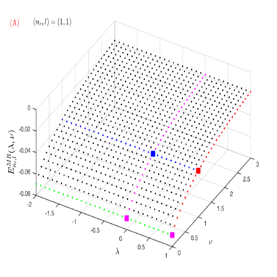
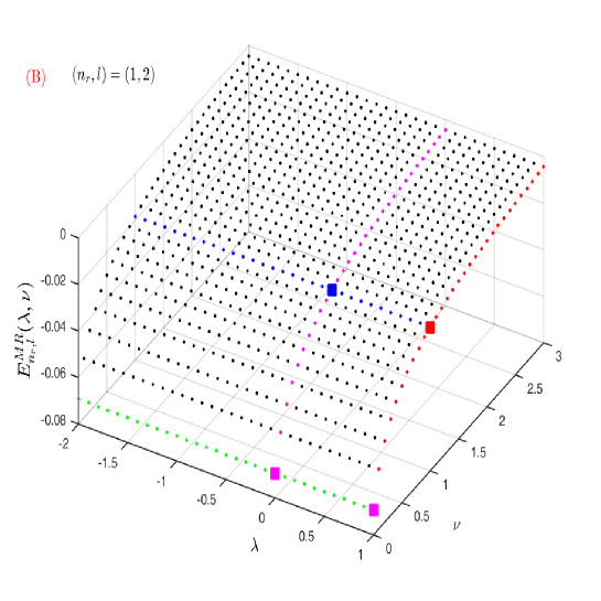
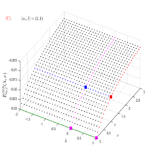
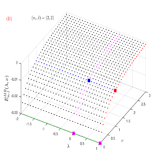
Figure 3: Effect of $\lambda$ and $\nu$ on the energy, $E_{n_{r},l}^{MR}$, of MR potential. Panels (A), (B), (C), (D) correspond to $(n_{r},l)$ values (1,1), (1,2), (2,1) and (2,2) respectively. The parameters are: $\hbar=\mu=1,\alpha=1.5,b=1/0.025$. See text for details.

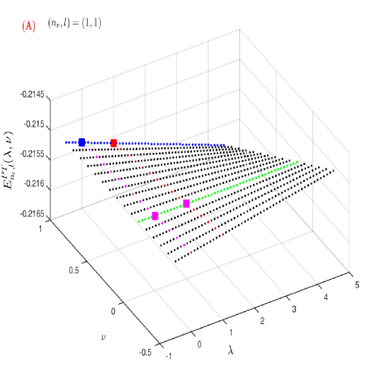
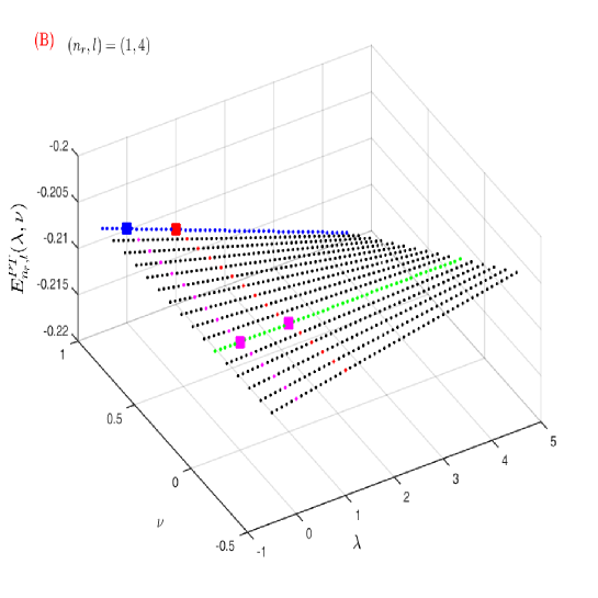
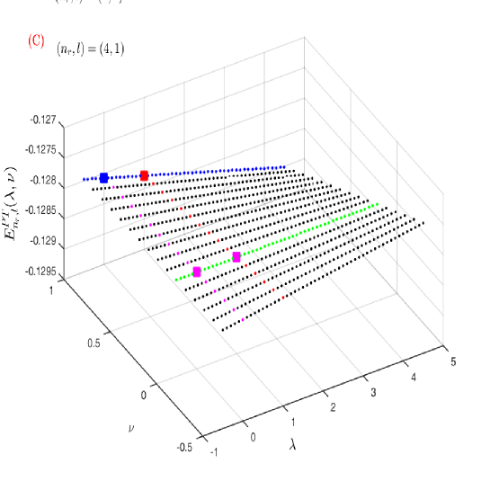
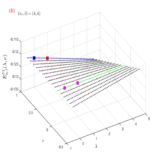
Figure 4: Effect of $\lambda$ and $\nu$ on the energy, $E_{n_{r},l}^{PT}$, of PT potential. Panels (A), (B), (C), (D) correspond to $(n_{r},l)$ values (1,1), (1,4), (4,1) and (4,4) respectively. The parameters are: $\hbar=\mu=1,\xi_{1}=4,\xi_{2}=2,\alpha=0.05$. See text for details.

References

- [1] M. F. Manning and N. Rosen, Phys. Rev. 44 (1933) 953.
- [2] A. Diaf, A. Chouchaoui and R. J. Lombard, Ann. Phys. 317 (2005) 354.
- [3] S.-H. Dong and J. García-Ravelo, Phys. Scr. 75 (2007) 307.
- [4] C.-Y. Chen, F.-L. Lu and D.-S. Sun, Phys. Scr. 76 (2007) 428.
- [5] W.-C. Qiang and S.-H. Dong, Phys. Lett. A 368 (2007) 13.
- [6] Z.-Y. Chen, M. Li and C.-S. Jia, Mod. Phys. Lett. A 24 (2009) 1863.
- [7] W. C. Qiang and S.-H. Dong, Phys. Scr. 79 (2009) 045004.
- [8] S. M. Ikhdair, Phys. Scr. 83 (2011) 015010.
- [9] A. Diaf and C. Chouchaoui, Phys. Scr. 84 (2011) 015004.
- [10] A. Abdel-Hady, Proc. of the 8th Conf. on Nucl. Particle Phys., NUPPAC-2011, Hurghada, Egypt (2011) 131.
- [11] I. Nasser, M. S. Abdelmonem and A. Abdel-Hady, Mol. Phys. 111 (2013) 1.
- [12] W. Lucha and F. F. Schöberl, Int. J. Mod. Phys. C 10 (1999) 607.
- [13] A. K. Roy, Mod. Phys. Lett. A 29 (2014) 1450042.
- [14] X.-Y. Gu and S.-H. Dong, J. Math. Chem. 49 (2011) 2053.
- [15] G. Pöschl and E. Teller, Z. Phys. 83 (1933) 143.
- [16] S. H. Dong, W. C. Qiang and J. Garcóa-Ravelo, Int. J. Mod. Phys. A 23 (2008) 1537.
- [17] W. C. Qiang and S.-H. Dong, Int. J. Quant. Chem. 110 (2010) 2342.
- [18] H. Yanar, A. Tas, M. Salti and O. Aydogdu, Eur. Phys. J. Plus. 135 (2020) 292.
- [19] R. Horchani, H. Jelassi, A. N. Ikot and U. S. Okorie, Int. J. Quant. Chem. (2020) e26558.
- [20] W. C. Qiang, W. L. Chen, K. Li and G. F. Wei, Phys. Scr. 79 (2009) 025005.
- [21] Y. You, F.-L. Lu, D.-S. Sun, C.-Y. Chen and S.-H. Dong, Few-Body Syst. 54 (2013) 2125.
- [22] C. L. Pekeris, Phys. Rev. 45 (1934) 98.
- [23] M. Badawi, N. Bessis and G. Bessis, J. Phys. B 5 (1972) L157.
- [24] W. C. Qiang, J. Y. Wu and S. H. Dong, Phys. Scr. 79 (2009) 065011.
- [25] F. J. S. Ferreira and F. V. Prudente, Phys. Lett. A 377 (2013) 3027.
- [26] R. L. Greene and C. Aldrich, Phys. Rev. A 14 (1976) 2363.
- [27] D. Nath and A. K. Roy, Int. J. Quant. Chem. 121 (2021) e26616. DOI: 10.1002/qua.26616
- [28] A. F. Nikiforov and V. B. Uvarov, Special Functions of Mathematical Physics. (Birkhäuser, Basel, 1988).
- [29] G. F. Wei, C. Y. Long and S. H. Dong, Phys. Lett. A 372 (2008) 2592.
- [30] H. I. Ahmadov, C. Aydin, N. S. H. Huseynova and O. Uzun, Int. J. Mod. Phys. E 22 (2013) 1350072.
- [31] B. J. Falaye, K. J. Oyewumi, T. T. Ibrahim, M. A. Punyasena and C. A. Onate, Can. J. Phys. 91 (2013) 98.
- [32] W. C. Qiang, K. Li and W. L. Chen, J. Phys. A 42 (2009) 205306.
- [33] M. C. Onyeaju, J. O. A. Idiodi, A. N. Ikot, M. Solaimani and H. Hassanabadi, J. Opt. 46 (2016) 254.
- [34] H. Louis, B. I. Ita and N. I. Nzeata, Eur. Phys. J. Plus 134 (2019) 315.
- [35] B. Khirali, A. K. Behera, J. Bhoi and U. Laha, Ann. Phys. (NY) 412 (2020) 168044.
- [36] G. F. Wei and S. H. Dong, Phys. Lett. A 373 (2008) 49.
- [37] S. M. Ikhdair and R. Sever, Ann. Phys. (Berlin) 17 (2008) 897.
- [38] I.S. Gradshteyn, I.M. Ryzhik, Tables of Integals, Series, and Products 5th edn (New York: Academic) 1994.
- [39] S. H. Dong, W. C. Qiang and J. García-Ravelo, Int. J. Mod. Phys. A 23 (2008) 1537.
- [40] A.K. Roy, Results Phys. 3 (2013) 103.
- [41] A.K. Roy, J. Math. Chem. 52 (2014) 1405.