Confined H^- ion within a density functional framework

Abstract

Ground and excited states of a confined negative Hydrogen ion has been pursued under Kohn-Sham density functional approach by invoking a physically motivated work-function-based exchange potential. The exchange-only results are of near Hartree-Fock quality. Local parameterised Wigner-type, and gradient- and Laplacian-dependent non-local Lee-Yang-Parr functionals are chosen to investigate the electron correlation effects. Eigenfunctions and eigenvalues are extracted by using a generalized pseudospectral method obeying Dirichlet boundary condition. Energy values are reported for 1s² (¹S), 1s2s (^3,1S) and 1s2p (^3,1P) states. Performance of the correlation functionals in the context of confinement is examined critically. The present results are in excellent agreement with available literature. Additionally, Shannon entropy and Onicescu energy are offered for ground and low lying singly excited 1s2s (³S) and 1s2p (³P) states. The influence of electron correlation is more predominant in the weaker confinement limit and it decays with an increase in confinement strength. In essence, energy and some information measures are estimated using a newly formulated density functional strategy.

Keywords: Shannon Entropy, Onicescu energy, quantum confinement, impenetrable boundary, excited states, hydride ion, exchange-correlation.

I Introduction

Atomic and molecular systems confined by different forms of external potentials show various novel and interesting properties which are significantly different from their free counterparts. Although the study of confined atoms started several decades earlier michels37 ; sommerfeld38 , spectroscopic analysis of energy levels and other structural properties of quantum systems under diverse external confinements have received attention in recent years laughlin09 ; sabin09 ; flores-riveros10 ; yakar11 ; montgomery13 ; bhattacharyya13 ; sen14 ; montgomery15 ; saha16 ; galvez17 ; jiao17 ; chandra18 . An atom under spatial constraints may be modeled for describing the effect of pressure on the system, which may impact the rearrangement of orbitals, energy spectrum, continuum lowering; also, bonding pattern and co-ordination number may undergo dramatic changes in a molecule. Interested reader can find some elegant reviews in the literature jaskolski96 ; sabin09 ; sen14 ; leykoo18 . Such changes in structure play a crucial role for gaining insight to the unusual physico-chemical properties in constrained systems. A systematic analysis of one- and two-electron atom/ion is, therefore, essential for a comprehensive understanding of quantum confinement.

A simple but interesting two-electron confined model is the hydrogen negative ion (H^-) restricted by a spherical barrier. Investigation on negative ions is an important research activity in atomic physics in their own right. Usually they are fragile quantum systems possessing binding energies less than one order of magnitude than that in the atom. H^- ion, in particular, plays a fundamental role in the understanding of effect of correlation in three-body quantum mechanical problems. As a result of this weaker binding, the correlation effects are rather sensitive and delicate, compared to an iso-electronic atom or positive ion. Several excellent reviews are available buckman94 ; miller17 on the subject. Almost eighty percent atoms are able to form stable negative ion. They play a dominant role in the context of electrical conductivity in weakly ionised gases and plasmas. The versatility of hydride ion has been well established. It acts as an efficient antioxidant in human body. In transition region of planetary nebula, it is present in high concentration. It also functions as the main source of opacity in sun atmosphere at red and infrared region. Unlike other negative ions, extensive theoretical study for H^- ion has been done since 1962. However similar works on its confined counterpart remains quite limited.

Most of the studies in literature have considered He atom as the prototypical two-electron confined system. Spatially confined H^- works are not so prevalent in literature, relatively speaking. Nevertheless, a decent number of methods exist. Some of these are: Hartree-Fock (HF) calculation with B-spline method wilson10 , a combination of quantum genetic algorithm and HF yakar11 , Hylleraas type wave function for variational calculation gimarc67 , quantum Monte Carlo joslin92 , CI calculation using explicitly correlated Hylleraas basis montgomery15 , for ground and singly excited S states. Apart from that, there prevails a couple of Rayleigh-Ritz approaches: (a) with three-parameter correlated wave function for ground state lesech11 (b) using explicitly correlated Hylleraas-type basis set for singly excited 1s2s and 1s3s (¹S) saha16 , for 1s² (¹S), 2p², 1snp (^1,3P) with (n = 2–5) (³P), in chandra18 . One also finds variational method based on (a) generalized Hylleraas basis (GHB) flores-riveros08 ; bhattacharyya13 and (b) B-splines basis tong-yun01 as well. A detailed analysis of electron correlation has been published in wilson10 . A density functional theory (DFT) report is available in sen05 , within LDA and BLYP functional. Penetrable walls have also been undertaken as well. For example, energy spectrum for different confinement strengths are analyzed for H^- ion confined by an anisotropic harmonic oscillator potential, by (i) CI method within gaussian basis sako03 (ii) adiabatic hyper-spherical approach fang07 . Other than energy, properties like static dipole polarizability holka05 ; choluj17 , second hyperpolarizability choluj17 for are also pursued. Energy levels and electric dipole polarizabilties of endohedrally confined H^- ion with CI method coupled with a B-spline approach are analyzed in melono18 . Some works are also reported in the context of H^- ion embedded in plasma environment zhang96 ; winkler96 ; kar04 ; kar05 ; kar07 ; kar08 ; kar08pla ; kar09 ; kar11 ; ho12 ; kar13 ; jiang13 ; jiao14 ; kar17 .

The relation between information theoretic tool and quantum mechanical kinetic energy was established in sear80 . Since then the importance of these measures in the context of DFT has been discussed in several papers romera04 ; romera05 ; nagy08 ; ghiringhelli10 ; nagy14a . In a recent work the Euler equation in orbital-free DFT is formulated by invoking Shannon entropy ($S$) and Fisher information nagy14 . Over the years these tools have emerged as versatile descriptors in analysing atoms and molecules guevara03 ; guevara05 ; moustakidis05 ; sen05 . They are functionals of density and can quantify it accurately in various complementary ways. In present work, we are specifically interested in two such measures, namely, Shannon entropy and Onicescu energy ($E$). The former is the arithmetic mean of uncertainty and can characterize a given density distribution in global way. The latter refers to the expectation value of density and generally complements the behavior of $S$. A decent amount of research work has been published to inspect these measures in free atom/ion. However, in confined situation, parallel reports are quite limited and scattered. One can mention the works on confined H atom (CHA), where $S$ was studied with change in $r_{c}$, in composite $r,p$ spaces, in case of both $l=0$ and non-zero $l$ states sen05 ; jiao17 ; mukherjee18 ; mukherjee18a . It was found that effect of confinement is more profound on higher states. Study of $S$ was also performed in sanchez19 for the hydrogen atom submitted to four different potentials: (a) infinite potential (b) Coulomb plus harmonic oscillator (c) constant potential and (d) dielectric continuum. In many-electron atoms, $S$ has been explored mostly using correlated Hylleraas-type wave function, in either attractive or repulsive conditions. Some DFT works are also reported. Thus ground state-$S$ was considered for two-electron iso-electronic series (H^- He, Li⁺, Be²⁺) under hard (impenetrable rigid wall) confinement, by using the BLYP XC functional sen05 ; another DFT study for ground and excited states is recently published in majumdar20 for He, Li$+$ and Be²⁺. Of late, there is a growing interest to treat the so-called finite (soft) confinement as well. Besides ground state, some limited works exist on low-lying excited states of $S$–mostly, for single ou17 and double ou17cpl excitations in He.

Thus it appears that there is a need for DFT calculation for confined many electron systems, in particular the negative ions. The motivation of the present work lies in that. Here we perform a detailed and systematic study of energy as well as $S,E$, in composite $r$ and $p$ spaces, for ground and some low-lying singly excited states of H^- ion, trapped inside high pressure environment. This is accomplished by invoking a simple work-function based exchange potential, motivated from physical grounds. The correlation effect is incorporated by using (i) a local, parameterized Wigner-type functional and (ii) the popular Lee-Yang-Parr (LYP) functional. The relevant KS differential equation under Dirichlet boundary condition is solved by adopting an accurate and efficient generalized pseudo-spectral (GPS) scheme. This procedure has been effectively applied to ground and a large number of excited states in free atoms as well as in some confinement works, with considerable success. Electron density, $S_{\mathrm{\mathbf{r}}},E_{\mathrm{\mathbf{r}}}$ are estimated from self-consistent orbitals. The momentum-space orbitals are obtained by performing Fourier transformation to $r$-space orbitals in usual way. Electron momentum density is constructed from $p$-space orbitals and subsequently $S_{\mathrm{\mathbf{p}}},E_{\mathrm{\mathbf{p}}}$ are obtained therefrom. Our pilot calculation are done on ground and 1s2s, 1s2p excited states. Section II sums up the adopted methodology. Section III imprints the calculated results along with a comparison with available references. Finally, Sec. IV concludes with the outlook and future prospects.

II Methodology

Here we briefly outline the proposed density functional method for a particular state of an arbitrary atom centered inside an impenetrable spherical cavity, followed by the GPS scheme for calculation of eigenvalues and energies of KS equation. This has been very successful for ground and various states (such as singly, doubly, triply excited states corresponding to low- and high-lying excitation, valence and core excitation, autoionizing, hollow, doubly hollow, Rydberg and satellite states etc.) of free or unconfined neutral atoms as well as ions roy97 ; roy97a ; roy97b ; roy02 ; roy04 ; roy05 ; roy07 . Very recently, this has been extended to confinement situations majumdar20 . Our focus remains on essential portions, omitting the relevant details, which are available in above references.

Our starting point is the non-relativistic single-particle time-independent KS equation with imposed confinement, which can be conveniently written as (atomic unit employed unless otherwise mentioned),

$$\left[-\frac{1}{2}\nabla^{2}+v_{eff}(\mathrm{\mathbf{r}})\right]\phi_{i}(\mathrm{\mathbf{r}})=\varepsilon_{i}\phi_{i}(\mathrm{\mathbf{r}}),$$ (1)

where the “effective” potential is constituted of following terms,

$$v_{eff}(\mathrm{\mathbf{r}}) = v_{ne}(\mathrm{\mathbf{r}})+\int\frac{\rho(\mathrm{\mathbf{r}}^{\prime})}{|\mathrm{\mathbf{r}}-\mathrm{\mathbf{r}}^{\prime}|}\mathrm{d}\mathrm{\mathbf{r}}^{\prime}+\frac{\delta E_{xc}[\rho(\mathrm{\mathbf{r}})]}{\delta\rho(\mathrm{\mathbf{r}})}+v_{conf}(\mathrm{\mathbf{r}}).$$ (2)

In this equation, the first three terms in right-hand site correspond to usual electron-nuclear attraction, classical Hartree repulsion and XC potentials respectively. The following perturbation accounts for the desired confinement ($r_{c}$ refers to the radius of spherical cage),

$$v_{conf}(\mathrm{\mathbf{r}})=\begin{cases}0,\ \ \ \ \ \ \ r\leq r_{c}\\ +\infty,\ \ \ \ r>r_{c}.\\ \end{cases}$$ (3)

Despite the remarkable progress and success in ground-state electronic structure and properties of atoms/molecules, in past five decades, excited state-DFT has faced difficulties and challenges. This is mainly due to lack of (i) an analogous Hohenberg-Kohn theorem and (ii) an accurate, proper XC functional for a general excited state. This work intends to employ an exchange potential sahni90 ; sahni92 , which is derived from physical grounds. Accordingly, one can interpret exchange energy as resulting from an interaction between an electron at $\mathrm{\mathbf{r}}$ and its Fermi-Coulomb hole charge density $\rho_{x}(\mathrm{\mathbf{r}},\mathrm{\mathbf{r}}^{\prime})$ at $\mathrm{\mathbf{r}}^{\prime}$. Thus it is given by,

$$E_{x}[\rho(\mathrm{\mathbf{r}})]=\frac{1}{2}\int\int\frac{\rho(\mathrm{\mathbf{r}})\rho_{x}(\mathrm{\mathbf{r}},\mathrm{\mathbf{r}}^{\prime})}{|\mathrm{\mathbf{r}}-\mathrm{\mathbf{r}}^{\prime}|}\ \mathrm{d}\mathrm{\mathbf{r}}\ \mathrm{d}\mathrm{\mathbf{r}}^{\prime}.$$ (4)

The unique local exchange potential $v_{x}(\mathrm{\mathbf{r}})$ for a given state, can then be defined as the work done in bringing an electron to the point $\mathrm{\mathbf{r}}$ against the electric field arising out of its Fermi-Coulomb hole density, leading to the following form,

$$v_{x}(\mathrm{\mathbf{r}})=-\int_{\infty}^{r}\mathcal{E}_{x}(\mathrm{\mathbf{r}})\mathrm{d}l,$$ (5)

where the electric field may be defined as,

$$\mathcal{E}_{x}(\mathrm{\mathbf{r}})=\int\frac{\rho_{x}(\mathrm{\mathbf{r}},\mathrm{\mathbf{r}}^{\prime})(\mathrm{\mathbf{r}}-\mathrm{\mathbf{r}}^{\prime})}{|\mathrm{\mathbf{r}}-\mathrm{\mathbf{r}}^{\prime}|^{3}}\ \mathrm{d}{\mathrm{\mathbf{r}}^{{}^{\prime}}}.$$ (6)

One can write the Fermi hole in terms of orbitals as,

$$\rho_{x}(\mathrm{\mathbf{r}},\mathrm{\mathbf{r}}^{\prime})=-\frac{\left|\gamma(\mathrm{\mathbf{r}},\mathrm{\mathbf{r}}^{\prime})\right|^{2}}{2\rho(\mathrm{\mathbf{r}})},$$ (7)

where $\left|\gamma(\mathrm{\mathbf{r}},\mathrm{\mathbf{r}}^{\prime})\right|=\sum_{i}\phi_{i}^{*}(\mathrm{\mathbf{r}})\phi_{i}(\mathrm{\mathbf{r}}^{\prime})$ is single-particle density matrix, while $\rho(\mathrm{\mathbf{r}})$ corresponds to electron density, expressed in terms of occupied orbitals ($n_{i}$ implies occupation number) as,

$$\rho(\mathrm{\mathbf{r}})=\sum_{i=1}^{N}n_{i}|\phi_{i}(\mathrm{\mathbf{r}})|^{2}.$$ (8)

While $v_{x}(\mathrm{\mathbf{r}})$ thus defined above, can be accurately calculated, one needs to approximate the unknown correlation potential $v_{c}(\mathrm{\mathbf{r}})$ for practical calculations. For this purpose, we employ two correlation functionals, namely, a Wigner-type brual78 and LYP lee88 . They have been chosen on the basis of their success in the context of excited states, which are recorded in the references roy97 ; roy97a ; roy97b ; roy02 ; roy04 ; roy05 ; roy07 . This will give the opportunity to examine and calibrate the performance of these functionals in current situation.

By taking the $v_{x}(\mathrm{\mathbf{r}})$ and $v_{c}(\mathrm{\mathbf{r}})$ as above, we proceed towards the solution of resulting KS equation following the Dirichlet boundary condition. This is done here by adopting an accurate and efficient GPS prescription, providing a non-uniform, optimal spatial discretization. It is a simple but effective method giving excellent results on numerous physically and chemically relevant problems, such as singular and non-singular roy02 ; roy04 ; roy05 ; roy07 ; roy04a ; roy04b ; roy05a ; roy05b , Coulomb, Húlthen, Yukawa, logarithmic, spiked oscillator, Hellmann potential, etc., along with its recent extension to quantum confinement sen06 ; roy15 ; roy16 . Since the details are well established and documented, we skip these here and refer the interested reader to the references above.

The numerical $p$-space wave function is obtained by Fourier transforming of $r$-space counterpart, as follows,

$$\xi(\mathrm{\mathbf{p}}) = \int\phi(\mathrm{\mathbf{r}})\ e^{i{\mathrm{\mathbf{p}}}.{\mathrm{\mathbf{r}}}}\mathrm{d}{\mathrm{\mathbf{r}}}.$$ (9)

Here, $\xi(\mathrm{\mathbf{p}})$ needs to be normalized. The normalized $r$- and $p$-space densities are then expressed in the forms as $\rho(\mathrm{\mathbf{r}})=\sum_{i=1}^{N}n_{i}|\phi_{i}(\mathrm{\mathbf{r}})|^{2}$ and $\Pi(\mathrm{\mathbf{p}})=\sum_{i=1}^{N}n_{i}|\xi_{i}(\mathrm{\mathbf{p}})|^{2}$ respectively, where $n_{i}$ indicates the occupation number of the $i$th orbital.

Next, $S_{\mathrm{\mathbf{r}}},~{}S_{\mathrm{\mathbf{p}}}$ and Shannon entropy sum $S_{t}$ are defined as given below,

$$S_{\mathrm{\mathbf{r}}} =-\int_{{\mathcal{R}}^{3}}\rho(\mathrm{\mathbf{r}})\ \ln[\rho(\mathrm{\mathbf{r}})]\ \mathrm{d}\mathrm{\mathbf{r}},\ \ \ S_{\mathrm{\mathbf{p}}}=-\int_{{\mathcal{R}}^{3}}\Pi(\mathrm{\mathbf{p}})\ \ln[\Pi(\mathrm{\mathbf{p}})]\ \mathrm{d}\mathrm{\mathbf{p}},$$ (10)

$$S_{t} =\left[S_{\mathrm{\mathbf{r}}}+S_{\mathrm{\mathbf{p}}}\right]\geq 3(1+\ln\pi),\ \ \ \ \ \text{in 3 dimension}.$$

Here both $\rho(\mathrm{\mathbf{r}})$ and $\Pi(\mathrm{\mathbf{p}})$ are normalized to unity.

All the computations are done numerically. The convergence is ensured by carrying out calculations with respect to variation in grid parameters, such as total number of radial points and maximum range of grid. It is generally observed that convergence is achieved relatively easily in the lower $r_{c}$ region compared to the $r_{c}\rightarrow\infty$ limit. All the quantities given in following tables and plots have been checked for above convergence.

Table 1: Ground-state energy of radially confined H^- for different $r_{c}$. See text for details.

$r_{c}$	X-only	Literature	XC-Wigner	XC-LYP	Literature
0.05	3885.9257	3885.925658	3885.7425	3887.3010	3885.922469, 3885.870899,
0.1	955.9361		955.7694	956.7881
0.4	53.8264		53.7168	54.0735	54.145, 54.3573
0.5	33.1632	33.18974	33.0645	33.3253	33.1120, 33.435, 33.11307
0.7	15.5897	15.59244	15.5072	15.7069	15.5400, 15.756, 15.54087
0.9	8.6106	8.61166	8.5395	8.6853	8.5621, 8.7073, 8.56299
1.0	6.6375	6.637526,6.64209	6.5709	6.6969	6.633326, 6.589644, 6.5897,
					6.7133, 6.59047
1.2	4.1341	4.13699	4.0749	4.1706	4.0875, 4.1826, 4.1492,
					4.08820
1.4	2.6808	2.68124	2.6275	2.7011	2.6354, 2.7112, 2.63603
1.8	1.1764	1.17666	1.1315	1.1758	1.1330, 1.1834, 1.13357
2.0	0.7665	0.76664	0.7248	0.7591	0.7240, 0.7231, 0.7245,
					0.7659, 0.7677, 0.72663
2.5	0.1799		0.1442	0.1616	0.1394,0.1388, 0.167
2.8	$-$0.0123		$-$0.0454	$-$0.0347	$-$0.051936, $-$0.051936
3.0	$-$0.1040	$-$0.10408	$-$0.1357	$-$0.1284	$-$0.1431, $-$0.1435, $-$0.143084,
					$-$0.124, $-$0.1427, $-$0.13915
					$-$0.14271, $-$0.143084
4.0	$-$0.3420	$-$0.34209	$-$0.3685	$-$0.3714	$-$0.3790, $-$0.3794, $-$0.379037,
					$-$0.369, $-$0.3786, $-$0.3295,
					$-$0.37464, $-$0.37875
5.0	$-$0.4258	$-$0.425815	$-$0.4493	$-$0.4564	$-$0.438594, $-$0.461974, $-$0.462073,
					$-$0.4620, $-$0.4623, $-$0.4617
					$-$0.456, $-$0.462073
6.0	$-$0.4595	$-$0.45954	$-$0.4813	$-$0.4902	$-$0.4958, $-$0.4958, $-$0.495772,
					$-$0.492, $-$0.4956, $-$0.4406,
					$-$0.49166, $-$0.49558
10.0	$-$0.4861	$-$0.486150,0.48614	$-$0.5056	$-$0.5157	$-$0.509209, $-$0.524688, $-$0.524688,
					$-$0.5247,$-$0.5239, $-$0.5245,
					$-$0.523, $-$0.52455, $-$0.524688
$\infty$	$-$0.4879	$-$0.487930, $-$0.48793	$-$0.5070	$-$0.5177	$-$0.514489, $-$0.527748,
					$-$0.5277, $-$0.5278, $-$0.528,
					$-$0.52775, $-$0.52481, $-$0.527751

aRef. wilson10 .	bRef. yakar11 .	cE${}^{1}_{RL}$ result of Ref. wilson10 .	dE2 result of Ref. wilson10 .	eRef. flores-riveros08 .
fRef. joslin92 .	gRef. sen05 .	hRef. chandra18 .	iRef. ting-yun01 .	jRef. gimarc67 .	kRef. marin92 .
lRef. lesech11 .	mRef. melono18 .	nRef. bhattacharyya13 .

III Result and Discussion

At the onset it is convenient to mention a few general comments about the conferred results for compressed H^- ion. Non-relativistic energies will be reported for ground 1s^{2 1}S and low lying single excited 1s2s ^3,1S, 1s2p ^3,1P states. Results on $S,E$ in composite r- and p-spaces will be presented for 1s^{2 1}S, 1s2s ³S and 1s2p ³P states. All results are in atomic units, unless stated otherwise. In order to organize the data in an appropriate manner, three sets of energies are attempted, viz., (i) exchange-only (ii) involving Wigner correlation (iii) considering LYP correlation. Throughout the discussion, these are termed as X-only, XC-Wigner and XC-LYP. Ground-state energies for confined H^- ion investigated with some interest. Consequently a healthy amount of literature is available and they are compared with the present calculation whenever feasible. However, for excited state such attempt is very uncommon and only a handful of results are available to collate. Furthermore, investigation of $S$ and $E$ for confined H^- ion is very scarce. Except sen05 no such record is available for comparison.

Table 2: Energies of 1s2s ^3,1S states of radially confined H^- for different $r_{c}$. See text for details.

	3S				1S
$r_{c}$	X-only	XC-Wigner	XC-LYP	Literature	X-only	XC-Wigner	XC-LYP	Literature
0.1	2426.7390	2426.5730	2428.1661	-	2432.4082	2432.2422	2433.8353	-
0.2	596.4463	596.3056	597.2946	-	599.3149	599.1741	600.1631	-
0.5	90.4448	90.3468	90.8032	91.20906a	91.6346	91.5368	91.9931	-
0.6	61.6373	61.5482	61.9275	62.15161a	62.6411	62.5522	62.9314	-
0.9	25.8082	25.7377	25.9755	25.97643a	26.5030	26.4327	26.6703	-
1	20.4697	20.4037	20.6111	20.52687a, 20.4597b	21.1030	21.0372	21.2444	-
1.2	13.6038	13.5451	13.7057	13.64636a, 13.5938b	14.1451	14.0868	14.2470	-
1.4	9.5381	9.4853	9.6118	9.56340a, 9.5284b	10.0142	9.9618	10.0879	-
1.5	8.1075	8.0571	8.1699	-	8.5576	8.5077	8.6201	-
1.8	5.2038	5.1594	5.2406	5.22940a, 5.1946b	5.5936	5.5499	5.6305	-
2	3.9798	3.9387	4.0043	3.99015a, 3.9709b	4.3398	4.2993	4.3644	-
3	1.2171	1.1864	1.2093	1.22002a, 1.2095b	1.4879	1.4579	1.4802	-
4	0.3435	0.3184	0.3245	0.34429a, 0.3371b	0.5660	0.5410	0.5468	-
5	$-$0.02131	$-$0.04307	$-$0.04430	-	0.1626	0.1396	0.1389	-
6	$-$0.2004	$-$0.22004	$-$0.2243	$-$0.20046a, $-$0.2050b	$-$0.0537	$-$0.0759	$-$0.0781	-
8	$-$0.3567	$-$0.3738	$-$0.3772	-	$-$0.2743	$-$0.2945	$-$0.2873	-
10	$-$0.4181	$-$0.4338	$-$0.4307	-	$-$0.3737	$-$0.3913	$-$0.3682	-
15	$-$0.4689	$-$0.4831	-	-	$-$0.4562	$-$0.4706	-	-

aRef. yakar11 (X-only energies).

bRef. flores-riveros08 (Correlated energies).

III.1 Energy analysis

Let us begin the discussion with ground state energies of confined H^- ion given in Table 1 at certain representative $r_{c}$’s, starting from very strong confinement regime $(r_{c}=0.05)$ to free limit $(r_{c}\rightarrow\infty)$. Present X-only results are reported in second column. These outcomes are almost identical with HF results obtained by using B-spline approach employing zeroth order spherical Bessel function wilson10 . In this context, note that, an analogous agreement with HF calculation ludena78 is also observed in case of He-isoelectronic series and Li, Be atoms for which similar calculation has been done by the authors and it will be published soon majumdar20a . Apart from that, the X-only values are also compared by invoking a combined quantum genetic algorithm (QGA) and RHF method yakar11 . A slightly compromised matching is observed at $r_{c}\leq 1$ region. However similarity between these two results improves with rise in $r_{c}$. At moderate to large $r_{c}$ ($\geq 3$) both the results become identical. All these literature values are available in third column of Table 1.

Table 3: Energies of 1s2p ^1,3P states of radially confined H^- for different $r_{c}$. See text for details.

	3P				1P
$r_{c}$	X-only	XC-Wigner	XC-LYP	Literature	X-only	XC-Wigner	XC-LYP	Literature
0.1	1472.6466	1472.4815	1473.7385	-	1479.8278	1479.6627	1480.9194	-
0.2	360.5257	360.3864	361.1685	-	364.1099	363.9706	364.7524	-
0.5	53.9750	53.8797	54.2403	54.02876a	55.4003	55.3050	55.6653	-
0.6	36.6134	36.5270	36.8264	36.64832a	37.7986	37.7123	38.0113	-
0.9	15.0984	15.0309	15.2173	15.10315a	15.8830	21.3313	16.0016	-
1.0	11.9084	11.8453	12.0075	11.92050a	12.6126	16.6321	12.7114	-
1.2	7.8186	7.7629	7.8875	7.82685a	8.4022	10.7516	8.4708	-
1.4	5.4079	5.3580	5.4551	5.41271a	5.9051	7.3797	5.9521	-
1.5	4.5627	4.5152	4.6013	-	5.0252	6.2176	5.0636	-
1.8	2.8547	2.8133	2.8737	2.85748a	3.2360	3.9069	3.2547	-
2	2.1393	2.10104	2.1488	2.14134a	2.4796	2.9556	2.4889	-
3	0.5434	0.5153	0.5281	0.54437a	0.7585	0.8711	0.7430	-
4	0.04955	0.02665	2.59005	0.04969a	0.1981	0.2033	0.1743	-
5	$-$0.1555	$-$0.17539	$-$0.1817	$-$0.162030b	$-$0.0497	$-$0.0566	$-$0.0757	$-$0.087731b
6	$-$0.2586	$-$0.27669	$-$0.2850	$-$0.25855a, $-$0.264743b	$-$0.1832	$-$0.1943	$-$0.2083	$-$0.215790b
8	$-$0.3575	$-$0.3737	$-$0.3803	$-$0.362587b	$-$0.3199	$-$0.3332	$-$0.3364	$-$0.341509b
10	$-$0.3957	$-$0.4109	$-$0.4063	-	$-$0.3951	$-$0.4102	$-$0.4041	-
15	$-$0.4533	$-$0.4671	-	-	$-$0.4531	$-$0.4669	-	-

aRef. yakar11 (X-only energies).

bRef. chandra18 (Correlated energies).

The columns 4 and 5 of Table 1 now represent the Wigner and LYP energies respectively; with corresponding references in column 6. At strong confinement zone $(\approx r_{c}\leq 3)$, Wigner energies are lower compared to LYP. However, at moderate to large $r_{c}$ region an opposite behavior is seen. The difference between these two energies remains in the range of $-$0.0107 to 1.5585 Moving from free to confinement condition total energy increases. This happens mainly due to an abrupt rise in kinetic energy. In most cases (except $r_{c}=0.05,2.5,2.8,3$), either of the correlated present results (PR) shows appreciable agreement with explicitly correlated GHB wilson10 ; flores-riveros08 ; chandra18 ; gimarc67 ; bhattacharyya13 energies. In XC-Wigner and XC-LYP, the absolute deviations are 0.003$\%$-3.93$\%$ and 0.03$\%$-4.84$\%$ respectively. At $r_{c}=0.05$, Wigner energies show excellent agreement with reported results, but a slight deviation is seen relative to XC-LYP value. However, at $r_{c}=2.5,2.8,3$, PR diverge from literature. It is important to mention that, in almost all the cases XC-LYP values are higher than the best-possible results flores-riveros08 ; chandra18 ; gimarc67 ; bhattacharyya13 , but no such trend is seen in XC-Wigner. These references also suggest that, at small $r_{c}$ region, Wigner performs better than LYP, but the scenario reverses with weakening of confinement strength. At strong confinement region $(r_{c}<4)$ PR are smaller than BLYP energies given in sen05 . However, this pattern reverses at $r_{c}>4$ range. Interestingly, at $r_{c}=4$, Wigner and BLYP energies sen05 become almost identical. A similar situation arises for LYP functional at $r_{c}=5$. In essence both Wigner and LYP produce reasonably good agreement with the BLYP results sen05 , recording absolute deviations of 0.13$\%$-13.65$\%$ and 0.08$\%$-3.54$\%$ respectively. At certain $r_{c}$’s ($\geq 0.4$) these are also tallied with CI method coupled with a B-Spline approach melono18 . In this case, the absolute deviation involving Wigner and LYP are 0.14-4.91$\%$ and 0.64-10.02$\%$ successively. Besides these, PR produces good agreement with other correlated energies available in ting-yun01 ; marin92 ; lesech11 . It is needless to mention that, as usual both X-only and correlated energies abate with rise in $r_{c}$.

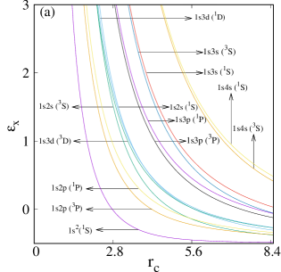
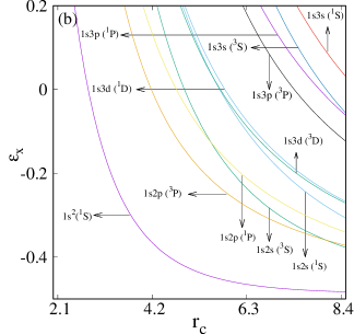
Figure 1: Energy changes in some low-lying states of confined H^- with $r_{c}$ in (a). Panel (b) shows a magnification of (a) in $\epsilon\leq 0.2$ region. See text for details.

Next, we move to employ this method in excited states. This provides an idea about its utility as well as performance in such states under hard confinement. Table 2 imprints energies of singly excited 1s2s ³S and ¹S states of a trapped H^- ion for a wide range of $r_{c}$. Reference theoretical results in this context, are very rare. To the best of our knowledge, both X-only and correlated results are available only for ³S state and no such values are reported for ¹S state. The second and sixth columns represent X-only results for triplet and singlet states. The X-only energies for ³S state can be compared with combined QGA-RHF method yakar11 and the results show good agreement. Similar to the ground state, here also the convergence between these two values increases with progress in $r_{c}$. Third and fourth columns of Table 2 offer the wigner and LYP energies for ³S, whereas columns six and seven provide the same for ¹S. Like the ground state, here also for both triplet and singlet states, LYP values are higher than Wigner data in $r_{c}\leq 5$ region. Further, in ³S, the matching between Wigner and LYP energies enhances with advancement in $r_{c}$. Absolute difference between these two correlated values for both the states are almost identical and it is in the range 0.003 to 1.593. Present correlated energies for triplet state are in good agreement with the available GHB results flores-riveros08 . In this case, absolute deviation for Wigner and LYP are 0.27-7.33$\%$ and 0.016-9.41$\%$ successively. It may also be noted that, in both cases deviation is higher in large $r_{c}$ regime.

Table 4: Energy values of some singly excited singlet and triplet states in radially confined H^- at $r_{c}=0.1$. Energies are arranged in ascending order. See text for details.

Configuration	States	X-only	XC-Wigner	XC-LYP
1s2p	3P, 1P	1472.6466, 1479.8278	1472.4815, 1479.6627	1473.7385, 1480.9194
1s3d	3D, 1D	2127.2860, 2132.8279	2127.1219, 2129.8212	2128.6253, 2130.1494
1s2s	3S, 1S	2426.7390, 2432.4082	2426.5730, 2432.2422	2428.2661, 2433.8353
1s4f	3F, 1F	2909.1492, 2910.6018	2908.9858, 2910.4384	2910.7391, 2912.1918
1s3p	3P, 1P	3445.2211, 3448.2732	3445.0558, 3448.1079	3446.9466, 3449.9986
1s5g	3G, 1G	3815.8480, 3816.6892	3815.6851, 3816.5263	3817.6904, 3818.5316
1s4d	3D, 1D	4600.3498, 4602.1893	4600.1849, 4602.0245	4602.3665, 4604.2060
1s6h	3H, 1H	4844.9833, 4845.5142	4844.8208, 4845.3517	4847.0792, 4847.6102
1s3s	3S, 1S	4891.8255, 4894.0532	4891.6597, 4893.7214	4893.9043, 4896.1319
1s5f	3F, 1F	5891.7768, 5892.9728	5891.6124, 5892.6439	5894.0811, 5895.2772
1s7i	3I, 1I	5994.5782, 5994.9344	5994.4160, 5994.7722	5996.9280, 5997.2843
1s4p	3P, 1P	6403.9567, 6405.4891	6403.7913, 6405.3236	6406.3592, 6407.8914
1s8k	3K, 1K	7263.0203, 7263.2706	7262.8583, 7363.1086	7265.6245, 7265.8746
1s6g	3G, 1G	7317.1025, 7317.9240	7316.9384, 7317.7598	7319.6921, 7320.5136
1s5d	3D, 1D	8055.1773, 8056.2696	8055.0122, 8056.1044	8057.8952, 8058.9874
1s4s	3S, 1S	8343.8330, 8345.0383	8343.6671, 8344.8724	8346.6009, 8347.8063

After the successful attempt of the present method in 1s2s configuration we now arrive at 1s2p case to investigate its ³P and ¹P states under compression. Table 3 provides energies for these two states at same range of $r_{c}$ given in previous table. Similar to the earlier excited states, only a handful of literature is available and they are mentioned in the footnotes. As usual the X-only results for triplet and singlet states are given in columns two and six respectively. Again the ³P state corroborates with the QGA-RHF energies yakar11 . Moreover, akin to the previous two cases, the extent of convergence (with literature energies) promotes with growth in $r_{c}$. Here also no literature is available to check the ¹P results. Correlated energies for ³P and ¹P are presented in columns 3, 4 and 7, 8. The absolute difference between the two correlated results are 0.0046-1.257 and 0.0032-1.2567 respectively. Moreover, both values approach each other with relaxation in confinement. In either of the cases GHB results are available for $r_{c}=5,6,8$ chandra18 , which offer reasonable agreement with PR.

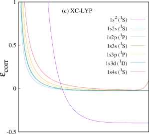
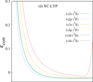
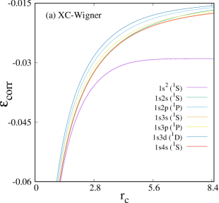
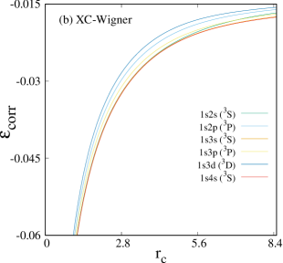
Figure 2: Correlation energies, with changes in $r_{c}$, for singly excited states of confined H^-, in panels (a) singlet (b) triplet states for Wigner correlation, while (c), (d) give same for LYP functional.

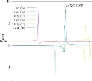
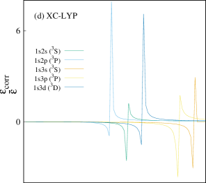
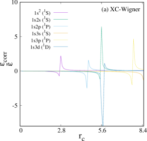
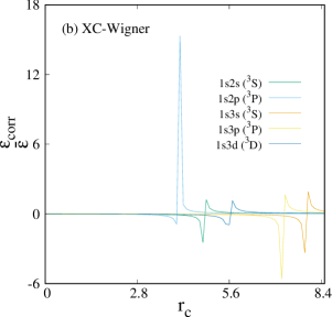
Figure 3: $\left(\frac{\epsilon_{corr}}{\epsilon}\right)$ for singly excited states of confined H^-, w.r.t. box size, in panels (a) singlet (b) triplet states for Wigner correlation, while (c), (d) give these for LYP functional.

These results of Tables 1–3 encourage us to investigate the impact of confinement on excited states in a qualitative manner. Therefore, such energies are plotted in panels (a) and (b) of Fig. 1 for a few singlet and triplet singly excited states as a function of $r_{c}$. In addition to the states investigated in above three tables, in this occasion, we have considered some additional states, such as, 1s3s and 1s4s ^3,1S, 1s3p ^3,1P and 1s3d ^3,1D. In order to get a better insight about the crossing amongst various states, an amplified region ($\epsilon\leq 0.2$) of panel (a) is demonstrated in panel (b) with improved resolution. X-only, XC-Wigner, XC-LYP energies generate qualitatively resembling plots. Hence, we take liberty to use X-only energies to point out some general features. In a free H^- ion the possible ordering of states under consideration is: $\epsilon_{\mathrm{1s4s}}(^{1}\mathrm{S})>$ $\epsilon_{\mathrm{1s4s}}(^{3}\mathrm{S})>$ $\epsilon_{\mathrm{1s3d}}(^{1}\mathrm{D})>$ $\epsilon_{\mathrm{1s3d}}(^{3}\mathrm{D})>$ $\epsilon_{\mathrm{1s3p}}(^{1}\mathrm{P})>$ $\epsilon_{\mathrm{1s3p}}(^{3}\mathrm{P})>$ $\epsilon_{\mathrm{1s3s}}(^{1}\mathrm{S})>$ $\epsilon_{\mathrm{1s3s}}(^{3}\mathrm{S})>$ $\epsilon_{\mathrm{1s2p}}(^{1}\mathrm{P})>$ $\epsilon_{\mathrm{1s2p}}(^{3}\mathrm{P})>$ $\epsilon_{\mathrm{1s2s}}(^{1}\mathrm{S})>$ $\epsilon_{\mathrm{1s2s}}(^{3}\mathrm{S})>$ $\epsilon_{\mathrm{1s}^{2}}(^{1}\mathrm{S})$. It has been found earlier that the influence of confinement seems to be more pronounced on valence orbitals leading to the rearrangement of atomic states at strong confinement regime montgomery15 ; majumdar20a . Once we move from free to confinement limit, multiple crossover between states occur, and the above order gets dissolved. This ordering is a function of $r_{c}$. From panel (a) it can be checked that at $r_{c}=4,~{}5.6,~{}7.2$ and 8.1 crossover between 1s2s ¹S, 1s3d ¹D; 1s2s ¹S, 1s3d ³D; 1s2s ³S, 1s2p ³P; 1s2s ³S, 1s2p ¹P occur respectively. Moreover, the last three crossings are clearly visible from panel (b). It is to be noted that, beyond the range of $r_{c}$ plotted here, several other crossings happen, which are not given this figure, to avoid clumsiness.

The outcomes of Fig. 1 motivate us to explore the ordering of various singly excited singlet and triplet states at strong confinement region. In this context, the energies for first thirty two singly excited triplet and singlet states arising from different singly excited configurations are provided in ascending order at $r_{c}=0.1$ in Table 4. The third, fourth and fifth columns provide the X-only, XC-Wigner and XC-LYP results respectively. It has been verified thoroughly that, apart from the presented states, no intermediate singly excited state can be found to lie in between them. It is to be noted here that, in this limit of confinement, for all the states under consideration, Hund’s rule is satisfied; singlet states possess higher energy than the triplets.

Table 5: $S_{\mathrm{\mathbf{r}}},S_{\mathrm{\mathbf{p}}}$ in ground state of confined H^-. See text for details.

$r_{c}$	X-only		XC-Wigner		XC-LYP		Literature
	$S_{\mathrm{\mathbf{r}}}$	$S_{\mathrm{\mathbf{p}}}$	$S_{\mathrm{\mathbf{r}}}$	$S_{\mathrm{\mathbf{p}}}$	$S_{\mathrm{\mathbf{r}}}$	$S_{\mathrm{\mathbf{p}}}$	$S_{\mathrm{\mathbf{r}}}$(a)	$S_{\mathrm{\mathbf{p}}}$(a)
0.1	$-$6.2407	12.847	$-$6.2407	12.8500	$-$6.2407	12.8500	-	-
0.2	$-$4.1701	10.7750	$-$4.1702	10.7750	$-$4.1701	10.7750	-	-
0.3	$-$2.9628	9.5621	$-$2.9629	9.5621	$-$2.9628	9.5621	$-$2.948	9.394
0.5	$-$1.4493	8.0373	$-$1.4495	8.0373	$-$1.4493	8.0373	$-$1.423	7.954
0.8	$-$0.06968	6.6413	$-$0.07027	6.6416	$-$0.06977	6.6413	$-$0.032	6.593
1	0.5781	5.9832	0.5771	5.9838	0.5779	5.9833	0.6209	5.943
1.2	1.1023	5.4494	1.1007	5.4503	1.1020	5.4495	1.1486	5.414
1.5	1.7353	4.8034	1.7327	4.8051	1.7347	4.8039	-	-
1.8	2.2430	4.2848	2.2391	4.2874	2.2421	4.2854	2.2912	4.255
2	2.5313	3.9904	2.5263	3.9940	2.5300	3.9913	2.5777	3.963
2.5	3.1253	3.3872	3.1171	3.3939	3.1230	3.3890	3.1633	3.366
3	3.5883	2.9228	3.5760	2.9337	3.5843	2.9263	3.6133	2.913
3.5	3.9583	2.5570	3.9409	2.5731	3.9517	2.5629	3.9672	2.563
4	4.2583	2.2653	4.2350	2.2876	4.2479	2.2750	4.2494	2.29
5	4.7051	1.8433	4.6675	1.8801	4.6818	1.8652	4.6607	1.908
7	5.2132	1.3942	5.1425	1.4627	5.1432	1.4570	5.1139	1.522
8	5.3524	1.2811	5.2657	1.3636	5.2568	1.3649	5.2423	1.423
10	5.5097	1.1623	5.3958	1.2666	5.3769	1.2755	-	-
15	5.6180	1.0911	5.4709	1.2180	5.4494	1.2309	-	-
25	5.6300	1.0852	5.4753	1.2162	5.4507	1.2330	-	-

(a)Ref. sen05 .

Table 6: $S_{\mathrm{\mathbf{r}}},S_{\mathrm{\mathbf{p}}}$ in 1s2s ³S and 1s2p ³P states of confined H^-. See text for details.

	1s2s 3S						1s2p 3P
$r_{c}$	X-only		XC-Wigner		XC-LYP		X-only		XC-Wigner		XC-LYP
	$S_{\mathrm{\mathbf{r}}}$	$S_{\mathrm{\mathbf{p}}}$	$S_{\mathrm{\mathbf{r}}}$	$S_{\mathrm{\mathbf{p}}}$	$S_{\mathrm{\mathbf{r}}}$	$S_{\mathrm{\mathbf{p}}}$	$S_{\mathrm{\mathbf{r}}}$	$S_{\mathrm{\mathbf{p}}}$	$S_{\mathrm{\mathbf{r}}}$	$S_{\mathrm{\mathbf{p}}}$	$S_{\mathrm{\mathbf{r}}}$	$S_{\mathrm{\mathbf{p}}}$
0.1	$-$6.21007	14.1888	$-$6.21007	14.1888	$-$6.21007	14.1888	$-$6.16304	13.0692	$-$6.16304	13.0711	$-$6.16304	13.0708
0.2	$-$4.13691	12.1115	$-$4.13691	12.1113	$-$4.1369	12.1112	$-$4.08845	10.9927	$-$4.08846	10.9927	$-$4.0884	10.9927
0.3	$-$2.92690	10.8967	$-$2.92692	10.8964	$-$2.9269	10.8977	$-$2.87704	9.7777	$-$2.87707	9.7722	$-$2.8770	9.7774
0.5	$-$1.40751	9.3668	$-$1.40758	9.3655	$-$1.4075	9.3671	$-$1.35498	8.2477	$-$1.35507	8.2474	$-$1.3549	8.2474
0.7	$-$0.41162	8.3593	$-$0.41177	8.3593	$-$ 0.4116	8.3592	$-$0.35658	7.2412	$-$0.35680	7.2411	$-$0.3566	7.2412
1	0.63727	7.2955	0.63690	7.2956	0.63721	7.2948	0.69568	6.1776	0.6951	6.1779	0.69559	6.1777
1.2	1.16957	6.7534	1.16902	6.7535	1.1694	6.7527	1.22992	5.6364	1.229152	5.6368	1.2297	5.6365
1.5	1.81613	6.0918	1.81523	6.0923	1.81598	6.0923	1.87883	4.9779	1.87755	4.9785	1.8785	4.9781
1.8	2.33915	5.5559	2.33780	5.5565	2.33891	5.5561	2.40340	4.4451	2.40149	4.4462	2.4029	4.4453
2	2.63865	0.1578	2.63697	5.2493	2.6383	5.2485	2.70343	4.1406	2.70102	4.1421	2.7028	4.1409
2.5	3.26448	4.6048	3.26181	4.6065	3.2639	4.6051	3.32850	3.5086	3.32455	3.5114	3.3275	3.5092
3	3.76475	4.0903	3.76088	4.0929	3.76398	4.0907	3.82454	3.0127	3.43221	3.4032	3.8228	3.0139
5	5.08159	2.7464	5.07112	2.7555	5.0747	2.7515	5.08496	1.8241	5.06728	1.8428	5.0721	1.8357
6	5.50678	2.3211	5.492351	2.3341	5.4877	2.3350	5.46497	1.5157	5.44087	1.5426	5.4369	1.5381
8	6.11312	1.7284	6.090808	1.7495	6.0292	1.7884	5.9898	1.1630	5.95727	1.2011	5.9018	1.2115
10	6.52773	1.3347	6.4987	1.3619	6.3378	1.4698	6.3630	0.9543	6.3269	0.9964	-	-
15	7.18923	0.7177	7.1486	0.7528	-	-	7.0703	0.5437	6.9781	0.6208	-	-
25	7.9460	$-$0.05128	7.8851	0.0932	-	-	7.8138	$-$0.00327	7.7680	0.04055	-	-

Till now we were involved in exploring the impact of confinement on total energy of H^- ion. It has been found that, both X-only and correlated energies diminish with increase in $r_{c}$ and merge to respective free limits. At this point, it is sensible to investigate the variation in correlation with change in confinement strength. In this regard, Wigner and LYP correlation energies are plotted in panels (a), (b) and (c), (d) of Fig. 2 respectively. The left panels (a), (c) represent corresponding singlet states and right panels (b), (d) indicate respective triplet states. From (a) and (b) it is evident that for both singlet and triplet states Wigner correlation energies accelerate with growth in $r_{c}$. This observation corroborates the pattern from a Hylleraas calculation wilson10 . Moreover, through out the range in $r_{c}$ the Wigner correlation energies remain negative for all these states. It is noteworthy that, correlation energy is the difference between exact energy and HF energy. Further, HF energy is always upper bound to the exact energy. Therefore, correlation energy should be negative. Here, Wigner correlation energies obey this criteria. Now we move to analyze the LYP correlation energy. On the contrary, from panels (c) and (d) it can be seen that, except for 1s4s ^3,1S states, LYP correlation energies for all other states decrease with progress in $r_{c}$. However, for 1s4s ^3,1S states it initially decreases with $r_{c}$, attains a flat minimum and then increases again. However, in the entire range of $r_{c}$ such energies for all these given states attain both positive as well as negative values.

We have also examined the ratio of correlation energy and respective total energy in Fig. 3 for Wigner (panels (a), (b)) and LYP (panels (c),(d)) functionals for the same set of excited states studied in Fig. 2. Here also panels (a), (c) refer to singlet states and (b), (d) signify triplet states. For each of these states involving either of the functionals, a sudden jump occurs at a characteristic $r_{c}$. This jump is not due to the sign change in either of the energies. Because, Wigner correlation energies are always negative, but LYP can be both positive and negative. Thus, for all these states these two energies connected to XC-Wigner changes their domain from negative correlation energy and positive total energy in low $r_{c}$ to negative correlation energy and negative total energy in free limit. However, for XC-LYP case, same change occurs from positive correlation energy and positive total energy region to negative correlation energy and negative total energy.

III.2 Shannon entropy and Onicescu energy

Now we apply this method to compute $S,E$ in conjugate $r$ and $p$ spaces. This gives a scope to verify and assess the quality of density in such states under hard confinement. Because, they act as descriptor in interpreting various chemical phenomena. Moreover, it will help us to understand the correlation contribution in present endeavor.

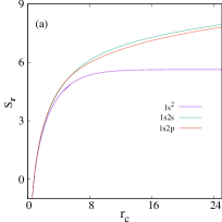
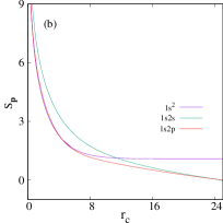
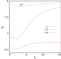
Figure 4: Variation of (a)$S_{\mathrm{\mathbf{r}}},(b)S_{\mathrm{\mathbf{p}}},(c)S_{t}$ with change in $r_{c}$ for H^- ion. See text for details.

Table 5 tabulates the numerical values of $S_{\mathrm{\mathbf{r}}}$ and $S_{\mathrm{\mathbf{p}}}$ for H^- ion in ground state at certain selected $r_{c}$ values. In all three occasions (X-only, XC-Wigner, XC-LYP) $S_{\mathrm{\mathbf{r}}}$ increases and $S_{\mathrm{\mathbf{p}}}$ decreases with growth in $r_{c}$. This amplifies the conclusion that, electron density gets compressed with strengthening of confinement effect. At strong confinement zone, both X-only and correlated results in either space become identical. However, with increase in $r_{c}$ this situation alters indicating the contribution of correlation effect in density. Similar observation was also reported in majumdar20 for He-isoelectronic series involving He, Li⁺ and Be⁺. At $r_{c}\geq 1$ regime, X-only values of $S_{\mathrm{\mathbf{r}}}$ are higher compared to both Wigner and LYP results. However, in $p$-space, a reverse behavior is noticed. X-only values are smaller relative to correlated results. The BLYP sen05 $S_{\mathrm{\mathbf{r}}}$ and $S_{\mathrm{\mathbf{p}}}$ are quoted in last two columns of table. The Wigner and LYP Shannon entropies are in complete correspondence with these cited values. It is evident that, $(S_{\mathrm{\mathbf{r}}}+S_{\mathrm{\mathbf{p}}})$ always remains greater that its limiting value of $3(1+\ln\pi)$.

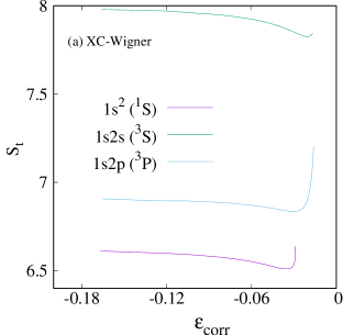
Figure 5: Variation of $S_{t}$ with change in correlation energy employing (a) XC-Wigner and (b) XC-LYP functional. See text for details.

Next, $S_{\mathrm{\mathbf{r}}}$, $S_{\mathrm{\mathbf{p}}}$ values for 1s2s ³S and 1s2p ³P states are reported in Table 6. The second to seventh columns represent ³S, whereas last six columns indicates ³P. No previous literature is available to match with our results. Analogous to the ground state, here also for either of the states, X-only and correlated entropies are uniform at strong confinement zone and the correlation contribution grows with rise in $r_{c}$. Further, at $r_{c}\geq 1$ region, the X-only results are comparatively higher than those from Wigner and LYP. It has been found that, at low to moderate $r_{c}$ region energies of 1s2s ³S state are larger than 1s2p ³P, and crossing occurs when $r_{c}$ value lies in between $5$ and $6$. However, an exactly opposite trend is encountered here in the context of $S_{\mathrm{\mathbf{r}}}$. These values for the former state is less than that of the latter, and a crossover happens at $r_{c}\approx 6$. However, $S_{\mathrm{\mathbf{p}}}$ obeys the same pattern as observed in energy. As usual the sum of $r$- and $p$-space $S$ is higher than the bound value of 6.43418.

Table 7: $E_{\mathrm{\mathbf{r}}},E_{\mathrm{\mathbf{p}}}$ in ground state of confined H^-. See text for details.

$r_{c}$	X-only		XC-Wigner		XC-LYP
	$E_{\mathrm{\mathbf{r}}}$	$E_{\mathrm{\mathbf{p}}}$	$E_{\mathrm{\mathbf{r}}}$	$E_{\mathrm{\mathbf{p}}}$	$E_{\mathrm{\mathbf{r}}}$	$E_{\mathrm{\mathbf{p}}}$
0.1	681.5854	0.000003	681.5874	0.000003	681.5855	0.000003
0.2	86.4424	0.00003	86.4442	0.00003	86.4426	0.00003
0.3	25.9984	0.0001	26.00007	0.0001	25.9985	0.0001
0.5	5.7942	0.0004	5.7956	0.0004	5.7944	0.0004
0.8	1.4880	0.0019	1.4892	0.0019	1.4882	0.0019
1	0.7901	0.0037	0.7911	0.0037	0.7902	0.0037
1.2	0.4751	0.0064	0.4761	0.0064	0.4753	0.0064
1.5	0.2588	0.0122	0.2597	0.0122	0.2590	0.0122
1.8	0.1601	0.0206	0.1610	0.0206	0.1396	0.0240
2	0.1224	0.0278	0.1232	0.0277	0.1226	0.0278
2.5	0.0713	0.0518	0.0721	0.0515	0.0715	0.0517
3	0.0476	0.0847	0.0484	0.0840	0.0479	0.0845
3.5	0.0350	0.1266	0.0358	0.1250	0.0353	0.1260
4	0.0277	0.1766	0.0285	0.1736	0.0281	0.1753
5	0.0202	0.2954	0.0211	0.2872	0.0207	0.2903
7	0.0151	0.5624	0.0162	0.5296	0.0160	0.5277
8	0.0142	0.6862	0.0154	0.6350	0.0153	0.6257
10	0.0135	0.8837	0.0147	0.7898	0.0147	0.7681
15	0.0132	1.1022	0.0145	0.9284	0.0144	0.9017
25	0.0132	1.1445	0.0143	0.9443	0.0145	0.9179

In order to get a better insight about the influence of confinement on entropies, $S_{\mathrm{\mathbf{r}}}$, $S_{\mathrm{\mathbf{p}}}$, $S_{t}$ are plotted as function of $r_{c}$, in panels (a)–(c) of Fig. 4, for 1s^{2 1}S, 1s2s ³S, 1s2p ³P states. The correlation effect does not alter the qualitative nature of the graph. Hence, X-only results suffice. As seen, $S_{\mathrm{\mathbf{r}}}$ progresses with gain in $r_{c}$, while $S_{\mathrm{\mathbf{p}}}$ declines. In conformity with Table VI, panel (a) also indicates the crossover between 1s2s ³S, 1s2p ³P states at around $r_{c}=6$. However, multiple crossovers between 1s^{2 1}S, 1s2s ³S; 1s^{2 1}S, 1s2p ³P are seen at $r_{c}\approx 6,11$ respectively in panel (b). $S_{t}$ in all these three cases, initially decline, then attain a minimum and finally increase.

In one-electron system, $S_{t}$ is independent of effective nuclear charge $Z$. However, in a many-electron system, this situation alters and it depends on $Z$. Previously $S_{t}$ was employed in explaining the correlation effect in both free and confined conditions guevara03 . Now, $S_{t}$ has been plotted as a function of correlation energy in Fig. 5. Panels (a)-(b) represent Wigner and LYP functionals. In the former case, for all these three states, it decays with rise in $\epsilon_{corr}$, then reaches a minimum and then sharply increases thereafter. On the contrary, for LYP functional involving 1s^{2 1}S, 1s2s ³S states, it sharply decreases to a minimum and then gradually increases with rise in $\epsilon_{corr}$. Further, for 1s2p ³P state, it always rises with $\epsilon_{corr}$.

Table 8: $E_{\mathrm{\mathbf{r}}},E_{\mathrm{\mathbf{p}}}$ in 1s2s ³S and 1s2p ³P states of confined H^-. See text for details.

	1s2s 3S						1s2p 3P
$r_{c}$	X-only		XC-Wigner		XC-LYP		X-only		XC-Wigner		XC-LYP
	$E_{\mathrm{\mathbf{r}}}$	$E_{\mathrm{\mathbf{p}}}$	$E_{\mathrm{\mathbf{r}}}$	$E_{\mathrm{\mathbf{p}}}$	$E_{\mathrm{\mathbf{r}}}$	$E_{\mathrm{\mathbf{p}}}$	$E_{\mathrm{\mathbf{r}}}$	$E_{\mathrm{\mathbf{p}}}$	$E_{\mathrm{\mathbf{r}}}$	$E_{\mathrm{\mathbf{p}}}$	$E_{\mathrm{\mathbf{r}}}$	$E_{\mathrm{\mathbf{p}}}$
0.1	898.6345	1$\times 10^{-8}$	898.6358	1$\times 10^{-8}$	898.6346	1$\times 10^{-8}$	931.7284	3$\times 10^{-7}$	931.7299	3 $\times 10^{-7}$	931.7285	3$\times 10^{-7}$
0.2	114.0409	1$\times 10^{-7}$	114.0421	1$\times 10^{-7}$	114.0410	1$\times 10^{-7}$	117.3172	2$\times 10^{-7}$	117.3185	2$\times 10^{-7}$	117.3173	2$\times 10^{-7}$
0.3	34.3147	3$\times 10^{-7}$	34.3158	3$\times 10^{-7}$	34.3148	3$\times 10^{-7}$	35.0239	9$\times 10^{-7}$	35.0251	9$\times 10^{-7}$	35.0240	9$\times 10^{-7}$
0.5	7.6508	1$\times 10^{-6}$	7.6517	1$\times 10^{-6}$	7.6509	1$\times 10^{-6}$	7.6867	4$\times 10^{-6}$	7.6876	4$\times 10^{-6}$	7.6868	4$\times 10^{-6}$
0.7	2.8815	4$\times 10^{-6}$	2.8823	4$\times 10^{-6}$	2.8816	4$\times 10^{-6}$	2.8497	12$\times 10^{-5}$	2.8505	12$\times 10^{-5}$	2.8498	12$\times 10^{-5}$
1	1.0408	13$\times 10^{-5}$	1.0415	13$\times 10^{-5}$	1.0409	13$\times 10^{-5}$	1.0055	3$\times 10^{-5}$	1.0062	3$\times 10^{-5}$	1.0056	3$\times 10^{-5}$
1.2	0.6244	2$\times 10^{-5}$	0.6250	2$\times 10^{-5}$	0.6245	2$\times 10^{-5}$	0.5941	6$\times 10^{-5}$	0.5947	6$\times 10^{-5}$	0.5942	6$\times 10^{-5}$
1.5	0.3382	4$\times 10^{-5}$	0.3388	4$\times 10^{-5}$	0.3384	4$\times 10^{-5}$	0.3148	0.0116	0.3153	0.0116	0.3149	0.0116
1.8	0.2077	8$\times 10^{-5}$	0.2082	8$\times 10^{-5}$	0.2078	8$\times 10^{-5}$	0.1893	0.0198	0.1898	0.0197	0.1894	0.0198
2	0.1578	1$\times 10^{-4}$	0.1583	1$\times 10^{-4}$	0.1579	1$\times 10^{-4}$	0.1420	0.0268	0.1425	0.0267	0.1421	0.0268
2.5	0.0900	0.0212	0.0905	0.0212	0.0901	0.0212	0.0789	0.0504	0.0794	0.0502	0.0790	0.0503
3	0.0585	0.0365	0.0590	0.0364	0.0586	0.0365	0.0504	0.0832	0.0719	0.0560	0.0506	0.0830
5	0.0215	0.1635	0.0219	0.1630	0.0217	0.1631	0.0199	0.2972	0.0204	0.2924	0.0202	0.2939
6	0.0166	0.2771	0.0170	0.2760	0.0169	0.2741	0.0171	0.4352	0.0177	0.4254	0.0175	0.4248
8	0.0126	0.6312	0.0130	0.6273	0.0132	0.5892	0.0162	0.7373	0.0170	0.7149	0.0166	0.6862
10	0.0112	1.1891	0.0169	1.1789	0.0121	0.9950	0.0166	1.0942	0.0175	1.0592	-	-
15	0.0102	3.7657	0.0108	3.7078	-	-	0.0175	2.5014	0.0184	2.4285	-	-
25	0.0100	16.3659	0.0106	15.7532	-	-	0.0179	9.2563	0.0189	8.9927	-	-

Now, we are interested to investigate $E$ in the same three representative (1s^{2 1}S, 1s2s ³S, 1s2p ³P) states of confined H^- ion. It generally complements $S$ by showing an opposite behavior. To the best of our knowledge, $E$ for confined H^- ion has never been investigated before. Therefore, in future, the present work may offer important guideline in this context.

Next, Table 7 provides $E_{\mathrm{\mathbf{r}}}$ and $E_{\mathrm{\mathbf{p}}}$ for H^- ion in ground state at the same $r_{c}$ values chosen in Table 5. X-only (columns 2, 3), Wigner (columns 4, 5) and LYP (columns 6, 7) results are given. $E_{\mathrm{\mathbf{r}}}$ progresses and $E_{\mathrm{\mathbf{p}}}$ abates with growth in $r_{c}$. At $r_{c}\rightarrow 0$ region, X-only and correlated results in both spaces become very similar. Akin to $S$, with increase in $r_{c}$ this situation alters implying the participation of correlation contribution in density. Then $E_{\mathrm{\mathbf{r}}}$, $E_{\mathrm{\mathbf{p}}}$ for 1s2s ³S and 1s2p ³P states are presented in Table 8. The arrangement is similar to Table 6. ³S values are given in second to seventh columns, while ³P results are given in last six columns. Similar to the ground state, here also for both states, the X-only and correlated results resemble each other at strong confinement limit. At low to moderate $r_{c}$ region, $E_{\mathrm{\mathbf{r}}}$ values of 1s2s ³S state lie higher than 1s2p ³P state and crossing occurs in between $r_{c}=$ 5 to 6. However, $E_{\mathrm{\mathbf{p}}}$ follows a reverse pattern.

Finally, $E_{\mathrm{\mathbf{r}}}$, $E_{\mathrm{\mathbf{p}}}$, $E_{t}$ for 1s^{2 1}S, 1s2s ³S, 1s2p ³P states are plotted as functions of $r_{c}$ in panels (a)-(c) of Fig. 6 respectively. As usual here also consideration of X-only results are sufficient to illustrate the essential purpose. $E_{\mathrm{\mathbf{r}}}$ declines with gain in $r_{c}$, while $E_{\mathrm{\mathbf{p}}}$ accelerates. As expected, multiple crossings between states takes place but they are not prominent from panel (a). However, panel (b) indicates the crossover between 1s^{2 1}S, 1s2s ³S and 1s^{2 1}S, 1s2p ³P. $E_{t}$ in all these three cases increase with $r_{c}$.

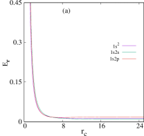
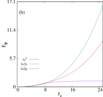
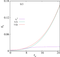
Figure 6: Variation of (a)$E_{\mathrm{\mathbf{r}}}(b)E_{\mathrm{\mathbf{p}}}(c)E_{t}$ with change in $r_{c}$ for H^- ion. See text for details.

IV Future and Outlook

An appropriate and effective KS DFT method is presented for calculation of H^- ion trapped inside an impenetrable spherical cavity of varying radius. The proposed recipe is computationally achievable and can easily be applied to other atoms in both ground and excited states. Energies are reported for ground and selected singly excited (1s2s ^3,1S, 1s2p ^3,1P) states of H^- ion in wide range of $r_{c}$ covering strong, moderate and weak confinement regime. Accurate results for a given state can be achieved, provided the exchange contribution is properly taken into account, which, of course, is the key reason behind the general success of this approach. Wigner correlation energies show qualitative similar behavior with the high-quality result of Hylleraas method. The results are generally in good agreement with the available literature. X-only results are very close to HF. A detailed investigation involving the singly excited states has been done to understand the rearrangement of atomic orbitals in strong confinement region.

In order to test the quality of the constructed density, $S,E$ in composite $r$ and $p$-spaces has been studied for ground and 1s2s ³S, 1s2p ³P states. To the best of our knowledge, this is the first reporting of information entropy in both ground and excited state of confined atoms in very strong confinement ($r_{c}\leq 0.1$) region. This study reinforces the previous conclusion majumdar20 that, at strong confinement zone, contribution of correlation effect in density is small. In order to increase the correctness and accuracy of the method, better correlation energy functionals are required to be designed and incorporated. In future present method may be extended to other atoms as well. Further, it is encouraging to probe the current procedure for other important realistic confinement scenario (such as encapsulation of an atom in supramolacular cavity). Investigation of multipole polarisability, atomic avoided crossing, hyperpolarisability, influence of electric and magnetic field through dynamical study is highly desirable, some of which may be undertaken later.

V Acknowledgement

Financial support from BRNS, India (sanction order: 58/14/03/2019-BRNS/10255) is gratefully acknowledged. SM is obliged to IISER-K for her Senior Research Fellowship. NM thanks CSIR, New Delhi, India, for a Senior Research Associateship (Pool No. 9033A).

References

- (1) A. Michels, J. de Boer, and A. Bijl. Physica, 4:981, 1937.
- (2) A. Sommerfeld and H. Welker. Ann. Phys., 32:56, 1938.
- (3) C. Laughlin and S. I. Chu. J. Phys. A, 42:265004, 2009.
- (4) J. Sabin, E. Brändas, and S. Cruz (Eds.). Adv. Quant. Chem., volume 57 & 58. Academic Press, New York, 2009.
- (5) A. Flores-Riveros, N. Aquino, and H. E. Montgomery Jr. Phys. Lett. A, 374:1246, 2010.
- (6) Y. Yakar, B. Çakir, and A. Özmen. Int. J. Quant. Chem., 111:4139, 2011.
- (7) H. E. Montgomery Jr., and V. I. Pupyshev. Phys. Lett. A, 377:2880, 2013.
- (8) S. Bhattacharyya, J. K. Saha, P. K. Mukherjee, and T. K. Mukherjee. Phys. Scr., 87:065305, 2013.
- (9) K. D. Sen (Ed.). Electronic Structure of Quantum Confined Atoms and Molecules. Springer International Publishing, Switzerland, 2014.
- (10) H. E. Montgomery Jr., and V. I. Pupyshev. Theor. Chem. Acc., 134:1598, 2015.
- (11) J. Saha, S. Bhattacharyya, and T. K. Mukherjee. Int. J. Quant. Chem., 116:1802, 2016.
- (12) F. J. Gálvez, E. Buendía, and A. Sarsa. Int. J. Quant. Chem., 117:e25421, 2017.
- (13) L. G. Jiao, L. R. Zan, Y. Z. Zhang, and Y. K. Ho. Int. J. Quant. Chem., 117:e25375, 2017.
- (14) R. Chandra, B. Dutta, J. K. Saha, S. Bhattacharyya, and T. K. Mukherjee. Int. J. Quant. Chem., 118:e25597, 2018.
- (15) W. Jaskólski. Phys. Rep., 271:1, 1996.
- (16) E. Ley-Koo. Revista Mexicana de Física, 64:326, 2018.
- (17) S. J. Buckman and C. W. Clark. Rev. Mod. Phys., 66:539, 1994.
- (18) T. J. Miller, C. Walsh, and T. A. Field. Chem. Rev., 117:1765, 2017.
- (19) C. L. Wilson, H. E. Montgomery Jr., K. D. Sen, and D. C. Thompson. Phys. Lett. A, 374:4415, 2010.
- (20) B. M. Gimarc. J. Chem. Phys., 47:5110, 1967.
- (21) C. Joslin and S. Goldman. J. Phys. B, 25:1965, 1992.
- (22) C. Le Sech and A. Banerjee. J. Phys. B, 44:105003, 2011.
- (23) A. Flores-Riveros and A. Rodríguez-Contreras. Phys. Lett. A, 372:6175, 2008.
- (24) S. Ting-Yun, B. Cheng-Guang, and L. Bai-Wen. Commun. Theor. Phys., 35:195, 2001.
- (25) K. D. Sen. J. Chem. Phys., 123:074110, 2005.
- (26) T. Sako and G. H. F. Diercksen. J. Phys. B, 36:1681, 2003.
- (27) W.-F. Xie. Commun. Theor. Phys., 47:1111, 2007.
- (28) F. Holka, P. Neogrády, V. Kellö, M. Urban, and G. H. F. Diercksen. Mol. Phys., 103:2747, 2005.
- (29) M. Chołuj, W. Bartkowiak, P. Nacikażek, and K. Strasburger. J. Chem. Phys., 146:194301, 2017.
- (30) R. L. Melingui Melono, C. F. Lukong, and O. Motapon. J. Phys. B, 51:205005, 2018.
- (31) Li. Zhang and P. Winkler. Int. J. Quant. Chem., 60:1643, 1996.
- (32) P. Winkler. Phys. Rev. E, 53:5517, 1996.
- (33) S. Kar and Y. K. Ho. Phys. Rev. E, 70:066411, 2004.
- (34) S. Kar and Y K Ho. New J. Phys., 7:141, 2005.
- (35) S. Kar and Y. K. Ho. Piers Online, 3:343, 2007.
- (36) S. Kar and Y. K. Ho. Phys. Plasmas, 15:013301, 2008.
- (37) S. Kar and Y. K. Ho. Phys. Lett. A, 372:4253, 2008.
- (38) S. Kar and Y. K. Ho. Phys. Rev. A, 80:062511, 2009.
- (39) S. Kar and Y. K. Ho. Phys. Rev. A, 83:042506, 2011.
- (40) Y. K. Ho and S. Kar. Few-Body Systems, 53:445, 2012.
- (41) S. Kar, H. W. Li, and P. Jiang. Phys. Plasmas, 20:083302, 2013.
- (42) P. Jiang, S. Kar, and Y. Zhou. Phys. Plasmas, 20:012126, 2013.
- (43) L. G. Jiao and Y. K. Ho. J. Quant. Spectrosc. Radiat. Transfer, 144:27, 2014.
- (44) S. Kar, Y.-S. Wang, Y. Wang, and Y. K. Ho. Int. J. Quant. Chem., 118:e25515, 2017.
- (45) S. B. Sears, R. G. Parr, and U. Dinur. Israel J. Chem., 19:165, 1980.
- (46) E. Romera and J. S. Dehesa. J. Chem. Phys., 120:8906, 2004.
- (47) E. Romera, P. Sánchez-Morena, and J. S. Dehesa. Chem. Phys. Lett., 414:468, 2005.
- (48) Á. Nagy and S. B. Liu. Phys. Lett. A, 372:1654, 2008.
- (49) L. M. Ghiringhelli, L. Delle, R. A. Mosna, and L. P. Hamilton. J. Math. Chem., 48:78, 2010.
- (50) Á. Nagy and E. Romera. Chem. Phys. Lett., 597:139, 2014.
- (51) Á. Nagy. Int. J. Quant. Chem., 115:1392, 2014.
- (52) N. L. Guevara, R. P. Sagar, and R. O. Esquivel. J. Chem. Phys., 119:7030, 2003.
- (53) N. L. Guevara, R. P. Sagar, and R. Q. Esquivel. J. Chem. Phys., 122:084101, 2005.
- (54) Ch. C. Moustakidis and S. E. Massen. Phys. Rev. B, 71:045102, 2005.
- (55) N. Mukherjee and A. K. Roy. Int. J. Quant. Chem., 118:e25596, 2018.
- (56) N. Mukherjee and A. K. Roy. Eur. Phys. J. D, 72:118, 2018.
- (57) M.-A. Martínez-Sánchez, R. Vargas, and J. Garza. Quant. Rep., 1:208, 2019.
- (58) S. Majumdar and A. K. Roy. Quant. Rep., 2:189, 2020.
- (59) J.-H. Ou and Y. K. Ho. Atoms, 5:15, 2017.
- (60) J.-H. Ou and Y. K. Ho. Chem. Phys. Lett., 689:116, 2017.
- (61) A. K. Roy, R. Singh, and B. M. Deb. J. Phys. B, 30:4763, 1997.
- (62) A. K. Roy, R. Singh, and B. M. Deb. Int. J. Quant. Chem., 65:317, 1997.
- (63) A. K. Roy and B. M. Deb. Phys. Lett. A, 234:465, 1997.
- (64) A. K. Roy and S. I. Chu. Phys. Rev. A, 65:052508, 2002.
- (65) A. K. Roy. J. Phys. B, 37:4369, 2004.
- (66) A. K. Roy. J. Phys. B., 38:1591, 2005.
- (67) A. K. Roy and A. F. Jalbout. Chem. Phys. Lett., 445:355, 2007.
- (68) V. Sahni and M. Harbola. Int. J. Quant. Chem. Symp., 24:569, 1990.
- (69) V. Sahni, Y. Li, and M. Harbola. Phys. Rev. A, 45:1434, 1992.
- (70) G. Brual and S. M. Rothstein. J. Chem. Phys., 69:1177, 1978.
- (71) C. Lee, Y. Wang, and R. G. Parr. Phys. Rev. B, 37:785, 1988.
- (72) A. K. Roy. Phys. Lett. A, 321:231, 2004.
- (73) A. K. Roy. J. Phys. G, 30:269, 2004.
- (74) A. K. Roy. Pramana-J. Phys., 38:2189, 2005.
- (75) A. K. Roy. Int. J. Quant. Chem., 104:861, 2005.
- (76) K. D. Sen and A. K. Roy. Phys. Lett. A, 357:112, 2006.
- (77) A. K. Roy. Int. J. Quant. Chem., 115:937, 2015.
- (78) A. K. Roy. Int. J. Quant. Chem., 116:953, 2016.
- (79) T.-Y. Si, C.-G. Bao, and B.-W. Li. Commun. Theor. Phys., 35:195, 2001.
- (80) J. L. Marín and S. A. Cruz. J. Phys. B, 25:4365, 1992.
- (81) E. V. Ludeña. J. Chem. Phys., 69:1770, 1978.
- (82) S. Majumdar and A. K. Roy. to be published.