ClusterEA: Scalable Entity Alignment with Stochastic Training and Normalized Mini-batch Similarities

Abstract.

Entity alignment (EA) aims at finding equivalent entities in different knowledge graphs (KGs). Embedding-based approaches have dominated the EA task in recent years. Those methods face problems that come from the geometric properties of embedding vectors, including hubness and isolation. To solve these geometric problems, many normalization approaches have been adopted for EA. However, the increasing scale of KGs renders it hard for EA models to adopt the normalization processes, thus limiting their usage in real-world applications. To tackle this challenge, we present ClusterEA, a general framework that is capable of scaling up EA models and enhancing their results by leveraging normalization methods on mini-batches with a high entity equivalent rate. ClusterEA contains three components to align entities between large-scale KGs, including stochastic training, ClusterSampler, and SparseFusion. It first trains a large-scale Siamese GNN for EA in a stochastic fashion to produce entity embeddings. Based on the embeddings, a novel ClusterSampler strategy is proposed for sampling highly overlapped mini-batches. Finally, ClusterEA incorporates SparseFusion, which normalizes local and global similarity and then fuses all similarity matrices to obtain the final similarity matrix. Extensive experiments with real-life datasets on EA benchmarks offer insight into the proposed framework, and suggest that it is capable of outperforming the state-of-the-art scalable EA framework by up to $8$ times in terms of $Hits@1$.

1. Introduction

Knowledge graphs (KGs) represent collections of relations between real-world objects, which facilitate many downstream applications, such as semantic search (Xiong et al., 2017) and recommendation systems (Zhang et al., 2016). Although various KGs have been constructed in recent years, they are still highly incomplete. To be more specific, KGs built from different data sources hold unique information individually while having overlapped entities. This motivates us to integrate the knowledge of different KGs with the overlapped entities to complete KGs. Entity alignment (EA) (Chen et al., 2017), a fundamental strategy for knowledge integration, has been widely studied. EA aims to align entities from different KGs that refer to the same real-world objects, and thus, it facilitates the completion of KGs.

Embedding-based EA has been proposed (Chen et al., 2017), and has been witnessed rapid development in recent years (Li et al., 2019; Mao et al., 2020b; Sun et al., 2020b, a; Mao et al., 2021a) thanks to the use of Graph Neural Networks (GNNs) (Kipf and Welling, 2017; Velickovic et al., 2018; Hamilton et al., 2017). They assume that the neighbors of two equivalent entities in KGs are also equivalent (Liu et al., 2020a). Based on this, they align entities by applying representation learning to KGs. We summarize the process of Embedding-based EA as the following three steps: (i) taking two input KGs and collecting seed alignment as training data; (ii) training an EA model with the isomorphic graph structure of two KGs to encode entities into embedding vectors; and (iii) aligning the equivalent entities between the two input KGs based on a specific similarity measurement (e.g., cosine similarity) of their corresponding embeddings.

The size of real-world KGs is much larger than that of conventional datasets used in evaluating EA tasks. For instance, a real-world KG YAGO3 includes 17 million entities (Ge et al., 2022). Thus, EA methods should be scaled up to massive data in order to adapt to real-world applications. However, a recent proposal (Ge et al., 2022) lost too much graph structure information, trading the quality of results for scalability. Worse still, as the input KGs become larger, using greedy search (Sun et al., 2020c) to find corresponding entities from one KG to another with top-1-nearest neighbor becomes more challenging. Specifically, the geometric properties of high-dimensional embedding vector spaces lead to problems for embedding-based EA, namely, geometric problems, mainly including the hubness and isolation problems (Sun et al., 2020c). The hubness problem indicates that some points (known as hubs) frequently appear as the top-1 nearest neighbors of many other points in the vector space. The isolation problem implies that some outliers would be isolated from any point clusters. As the scale of input KGs grows, these problems become even more severe due to the increasing number of candidates of nearest neighbor search. EA is generally assumed to follow 1-to-1 mapping (Chen et al., 2017). Many existing methods have been proposed to solve the geometric problems by making the similarity matrix better satisfy this assumption, i.e., normalization methods. A list of widely used normalization methods for EA includes (i) Cross-domain Similarity Local Scaling (CSLS) (Lample et al., 2018) that is adopted from word translation (Sun et al., 2019; Liu et al., 2020b; Mao et al., 2020b; Ge et al., 2021); (ii) Gale-Shapley algorithm (Roth, 2008) that treats EA as stable matching (Zeng et al., 2020a, 2021); (iii) Hungarian algorithm (Harold W. Kuhn, 1955) and (iv) Sinkhorn iteration (Cuturi, 2013) that both transform EA as the assignment problem (Fey et al., 2020; Mao et al., 2021b; Ge et al., 2021). Specifically, Sinkhorn iteration (Cuturi, 2013) could significantly improve the accuracy of matching entities with embeddings (Ge et al., 2021; Mao et al., 2021b). Moreover, Sinkhorn iteration suits the normalization approach of EA best as it can be easily parallelized on the GPU. Nonetheless, the existing normalization approaches (Lample et al., 2018; Cuturi, 2013; Roth, 2008; Harold W. Kuhn, 1955) are at least of quadratic complexity. This prohibits them from being applied to large-scale data, thus limiting their real-world applications.

In this work, we aim to scale up the normalization process of the similarity matrix to achieve higher EA performance. We adopt a standard machine learning technique, sampling mini-batches, to perform EA in linear time. Specifically, we first train a GNN model to obtain the global embeddings of two KGs. Then, we generate mini-batches for two KGs by placing entities that could find their equivalent together. Next, we calculate and normalize a local similarity matrix between two sets of entities selected for each mini-batch by Sinkhorn iteration. Finally, we merge the local similarities into a unified and sparse similarity matrix. With this strategy, the final similarity matrix is normalized with Sinkhorn iteration, thus achieving higher accuracy, and the time and space complexities can also be significantly reduced. However, its materialization is non-trivial due to the two major challenges:

• How to sample mini-batches with high entity equivalence rate to ensure 1-to-1 mapping? Splitting mini-batches on two KGs is quite different from conventional tasks. To transfer EA within mini-bathes into the assignment problem, we should place possibly equivalent entities into the same batch to meet the 1-to-1 mapping assumption. Nevertheless, the mapping is only partially known (as the training set) for the EA task, making it hard for two entities to be aligned and hence to be placed in the same batch. Intuitively, randomly splitting two KGs will make most mini-batches fail to correspond. An existing study (Ge et al., 2022) proposes a rule-based method to split batches with a higher rate of entity equivalence. Nonetheless, its results are still not enough to satisfy the 1-to-1 mapping assumption.

• How to fuse the mini-batch similarity matrices to ensure high accuracy? The similarity matrix of each batch focuses only on its local information. Thus, the results generally deviate from those obtained without sampling, even if the batch sampler is good enough. This motivates us to study two problems. First, how to combine the similarities of the mini-batches to get a better global optimal match, after getting the mini-batch. Second, how to improve the accuracy of results obtained by batch samplers.

To tackle the aforementioned two challenges, we present a general EA framework, ClusterEA, that can be applied to arbitrary GNN-based EA models while can be able to achieve high accuracy and scalability. To scale up GNN training over large-scale KGs, ClusterEA first utilizes neighborhood sampling (Hamilton et al., 2017) to train a large-scale GNN for EA in a stochastic fashion. Then, with the embedding obtained from the GNN model, ClusterEA proposes a novel strategy for generating high-quality mini-batches in EA, called ClusterSampler. As depicted in Figure 1, ClusterSampler first labels the training pairs into different batches with a clustering method. Then, it performs supervised classification using previously labeled training pairs to generate mini-batches for all the entities. By changing the clustering and classification models, the strategy can sample mini-batches by capturing multiple aspects of the graph structure information. We propose two sampling methods within ClusterSampler, including (i) Intra-KG Structure-based ClusterSampler (ISCS) that retains the intra-KG graph structure information such as the neighborhood of nodes; and (ii) Cross-KG Mapping-based ClusterSampler (CMCS) which retains the inter-KG matching information provided by the learned embedding. These methods sample two KGs into multiple mini-batches with a high entity equivalent rate to satisfy the 1-to-1 mapping assumption better. Finally, ClusterEA uses our proposed SparseFusion, which fuses the similarity matrices calculated separately using Sinkhorn iteration with normalized global similarity. The SparseFusion produces a matrix with high sparsity while keeping as much valuable information as possible.

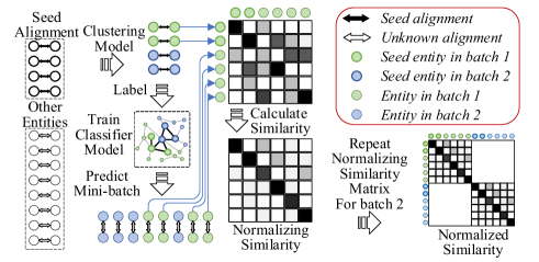
Figure 1. An example of normalizing mini-batch similarity matrix with ClusterSampler strategy

Our contributions are summarized as follows:

• Scalable EA framework. We develop ClusterEA, a scalable framework for EA, which reduces the complexity of normalizing similarity matrices with mini-batch. To the best of our knowledge, this is the first framework that utilizes stochastic GNN training for large-scale EA. Any GNN model can be easily integrated into ClusterEA to deal with large-scale EA (Section 4) with better scalability and higher accuracy.

• Fast and accurate batch samplers. We present ClusterSampler, a novel strategy that samples batches by learning the latent information from embeddings of the EA model. In the strategy, we implement two samplers to capture different aspects of KG information, including (i) ISCS that aims at retaining the intra-KG graph structure information, and (ii) CMCS that aims at retaining the inter-KG alignment information. Unlike the previous rule-based method, the two samplers are learning-based, and thus can be parallelized and produce high-quality mini-batches.

• Fused local and global similarity matrix. We propose SparseFusion for normalizing and fusing not only local similarity matrices but also global similarity matrices into one unified sparse matrix, which enhances the expressive power of EA models.

• Extensive experiments. We conduct comprehensive experimental evaluation on EA tasks compared against state-of-the-art approaches over the existing EA benchmarks. Considerable experimental results demonstrate that ClusterEA successfully achieves satisfactory accuracy on both conventional datasets and large-scale datasets (Section 5).

2. Related Work

Most existing EA proposals find equivalent entities by measuring the similarity between the embeddings of entities. Structures of KGs are the basis for the embedding-based EA methods. Representative EA approaches that rely purely on KGs’ structures can be divided into two categories, namely, KGE-based EA (Chen et al., 2017; Zhu et al., 2017; Sun et al., 2018, 2019) and GNN-based EA (Wang et al., 2018; Li et al., 2019; Mao et al., 2020a; Sun et al., 2020b, a; Cao et al., 2019). The former incorporates the KG embedding models (e.g., TransE (Bordes et al., 2013)) to learn entity embeddings. The latter learns the entity embeddings using GNNs (Kipf and Welling, 2017), which aggregates the neighbors’ information of entities.

In recent years, GNN-based models have demonstrated their outstanding performance (Mao et al., 2021a). This is contributed by the strong modeling capability on the non-Euclidean structure of GNNs with anisotropic attention mechanism (Velickovic et al., 2018). Nonetheless, they suffer from poor scalability (Ge et al., 2022) due to the difficulty in sampling mini-batches with neighborhood information on KGs. LargeEA (Ge et al., 2022), the first study focusing on the scalability of EA, proposes to train GNN models on relatively small batches of two KGs independently. The small batches are generated with a rule-based partition strategy called METIS-CPS. However, massive information of both graph structures and seed alignment is lost during the process, resulting in poor structure-based accuracy. In contrast, ClusterEA utilizes neighborhood sampling (Hamilton et al., 2017). Specifically, it trains one unified GNN model on the two KGs, during which the loss of structure information is neglectable. Moreover, ClusterEA creates mini-batches using multiple aspects of graph information, resulting in better entity equivalent rate than METIS-CPS.

In addition to structure information, many existing proposals facilitate the EA performance by employing side information of KGs, including entity names (Sun et al., 2017; Zhang et al., 2019; Fey et al., 2020; Zeng et al., 2020b; Tang et al., 2020; Liu et al., 2020a; Ge et al., 2021; Mao et al., 2021b; Ge et al., 2022; Azzalini et al., 2021; Zhao et al., 2022), descriptions (Zhang et al., 2019; Tang et al., 2020), images (Liu et al., 2020b), and attributes (Sun et al., 2017; Wang et al., 2018; Zhang et al., 2019; Yang et al., 2020; Tang et al., 2020; Liu et al., 2020a; Wang et al., 2020). Such proposals are able to mitigate the geometric problems (Sun et al., 2020c). Nonetheless, the models using side information mainly have two main limitations. First, side information may not be available due to privacy concerns, especially for industrial applications (Mao et al., 2021a, 2020b, 2020a). Second, models that incorporating machine translation or pre-aligned word embeddings may be overestimated due to the name bias issue (Chen et al., 2021; Liu et al., 2020a, b; Sun et al., 2021). Thus, compared with the models employing side information, the structure-only methods are more general and not affected by bias of benchmarks. To this end, we do not incorporate side information in ClusterEA.

In order to solve the geometric problems of embedding-based EA approaches, CSLS (Lample et al., 2018) have been widely adopted, which normalizes the similarity matrix in recent studies (Sun et al., 2019; Liu et al., 2020b; Mao et al., 2020b; Ge et al., 2021). However, CSLS does not perform full normalization of the similarity matrix. As a result, its improvement over greedy search of top-1-nearest neighbor is limited. CEA (Zeng et al., 2020a, 2021) adopts the Gale-Shapley algorithm (Roth, 2008) to find the stable matching between entities of two KGs, which produces higher-quality results than CSLS. Nevertheless, the Gale-Shapley algorithm is hard to be parallelized, and hence, it is almost infeasible to perform large scale EA. Recent studies have transformed EA into the assignment problem (Ge et al., 2021; Mao et al., 2021b). They adopt Hungarian algorithm (Harold W. Kuhn, 1955) or Sinkhorn iteration (Cuturi, 2013) to normalize the similarity matrix. However, the computational cost of such algorithms is high, prohibiting them from being applied to large scale EA. ClusterEA also utilizes Sinkhorn iteration (Cuturi, 2013) which performs full normalization on the similarity matrix with GPU acceleration. Moreover, ClusterEA develops novel batch-sampling methods for adopting the normalization to large-scale datasets with the loss of information being minimized.

3. Preliminaries

We proceed to introduce preliminary definitions. Based on these, we formalize the problem of entity alignment.

Definition 1.

A knowledge graph (KG) can be denoted as $G=(E,R,T)$, where $E$ is the set of entities, $R$ is the set of relations, and $T=\{(h,r,t)~{}|~{}h,t\in E,r\in R\}$ is the set of triples, each of which represents an edge from the head entity $h$ to the tail entity $t$ with the relation $r$.

Definition 2.

Entity alignment (EA) (Sun et al., 2020c) aims to find the 1-to-1 mapping of entities $\phi$ from a source KG $G_{s}=(E_{s},R_{s},T_{s})$ to a target KG $G_{t}=(E_{t},R_{t},T_{t})$. Formally, $\phi=\{(e_{s},e_{t})\in E_{s}\times E_{t}~{}|~{}e_{s}\equiv e_{t}\}$, where $e_{s}\in E_{s}$, $e_{t}\in E_{t}$, and $\equiv$ is an equivalence relation between $e_{s}$ and $e_{t}$. In most cases, a small set of equivalent entities $\phi^{\prime}\subset\phi$ is known beforehand and used as seed alignment.

Definition 3.

Embedding-based EA aims to learn a set of embeddings for all entities $E_{s}$ and $E_{t}$, denoted as $\mathbf{f}\in\mathcal{R}^{(|E_{s}|+|E_{t}|)\times D}$, and then, it tries to maximize the similarity (e.g. cosine similarity) of entities that are equivalent in $\phi$, where $D$ is the size of embedding vectors.

4. Our Framework

In this section, we present our proposed framework ClusterEA, a novel scalable EA framework. We start with the overall framework, followed by details on each component of our framework.

4.1. Overall Framework of ClusterEA

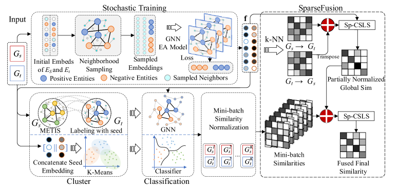
Figure 2. The overall ClusterEA framework

As shown in Figure 2, to scale up GNN training over large-scale KGs, ClusterEA first utilizes neighborhood sampling (Hamilton et al., 2017) to train a large-scale GNN for EA in a stochastic fashion. Thereafter, ClusterEA proposes a novel learning-based batch sampling strategy ClusterSampler. It uses the embedding vectors obtained from stochastic training. In the strategy, two batch samplers that learn multiple aspects of the input KGs are applied to the input KGs, including (i) ISCS that aims at retaining the intra-KG graph structure information such as the neighborhood of nodes, and (ii) CMCS that aims at retaining the inter-KG matching information provided by the learned embedding. These methods sample two KGs into multiple mini-batches with a high entity equivalent rate that better satisfies the 1-to-1 mapping assumption. Finally, ClusterEA proposes SparseFusion, which fuses the normalized local similarity matrices with partially normalized global similarity. The SparseFusion produces the fused final matrix with high sparsity while keeping as much valuable information as possible.

4.2. Stochastic Training of GNNs for EA

GNN-based methods (Liu et al., 2020a; Li et al., 2019; Liu et al., 2020b; Sun et al., 2020b; Mao et al., 2021a) have dominated the EA tasks with promising performances by propagating the information of seed alignments to their neighbors. Inspired by this, we propose to incorporate GNN-based models into ClusterEA. ClusterEA provides a general framework for training a Siamese GNN on both $G_{s}$ and $G_{t}$ that all GNN-based EA models follow (Mao et al., 2021a). As a result, any existing GNN model can be used in ClusterEA to produce the structural feature embeddings of entities.

To scale up the existing GNN-based EA models, ClusterEA trains the models with neighborhood sampling. We sample mini-batches based on the seed alignment. Specifically, following the negative sampling process, we first randomly select a mini-batch of size $N_{p}$ containing source and target entities $\phi_{s}^{\prime}$ and $\phi_{t}^{\prime}$ in the seed alignment $\phi^{\prime}$ that are equivalent. Then, we randomly sample source and target entities size of $N_{n}$ with seed alignment in their whole entity sets that does not overlap with selected seed entities, denoted as $\theta_{s}=\{e_{s}|e_{s}\in E_{s}\cap e_{s}\not\in\phi_{s}^{\prime}\}$ and $\theta_{t}=\{e_{t}|e_{t}\in E_{t}\cap e_{t}\not\in\phi_{t}^{\prime}\}$. Finally, a mini-batch $B=\{B_{s},B_{t}\}=\{(\phi_{s}^{\prime}\cup\theta_{s}),(\phi_{t}^{\prime}\cup\theta_{t})\}$ is generated waiting for the GNN model to produce its embeddings.

Generally, the GNN-based models train the entity’s embedding by propagating the neighborhood information (Mao et al., 2020b; Kipf and Welling, 2017; Velickovic et al., 2018). Formally, the embedding of an entity $v\in B$ in the $k_{th}$ layer of GNN $h_{v}^{k}$ is obtained by aggregating localized information via

(1) $$\begin{array}[]{c}a_{v}^{(k)}=\operatorname{Aggregate}^{(k)}(\left\{h_{u}^{(k-1)}\mid u\in\mathcal{N}(v)\right\})\\ h_{v}^{(k)}=\operatorname{Update}^{(k)}(a_{v}^{(k)},h_{v}^{(k-1)})\end{array}\vspace{-1mm}$$

where $h_{v}^{0}\in\mathcal{R}^{D}$ is a learnable embedding vector initialized with Glorot initialization, and $\mathcal{N}(v)$ represents the set of neighboring entities around $v$. The model’s final output on entity $e$ is denoted as $\mathbf{f}_{e}$. By applying neighborhood sampling, the size of neighborhood in each GNN layer of each entity is limited that no more than a fan out hyperparameter $F$, formally $|\mathcal{N}(v)|\leq F$. We place the graph information on CPU memory. When computing one layer of GNN in each batch, the neighbor of entities in current batch is sampled to form a block of graph, the graph information of this block will be transferred to GPU memory, along with the computation graph, making the final loss backward propagated with GPU.

To maximize the similarities of equivalent entities in each mini-batch, GNN-based EA models often use triplet loss along with negative sampling (Wang et al., 2018; Li et al., 2019; Mao et al., 2020b, a). In this paper, the Normalized Hard Sample Mining (NHSM) loss (Mao et al., 2021a), an extension for negative sampling that could significantly reduce training epochs, is adopted by us for training large-scale GNNs. We detail how we apply the NHSM loss in Appendix A.

Discussions. Due to the neighborhood sampling process, our stochastic version of EA training will have a certain graph information loss, which is minimized with the randomness of sampling. Recent studies (Chiang et al., 2019) have proposed to limit the sampling in small fixed sub-graphs for better training speed, which will further decrease the accuracy. LargeEA (Ge et al., 2022), on the other hand, trains multiple GNNs on small batches generated with a rule-based method. Such an approach could fasten the training process. Nonetheless, much of the structure information is lost during partitioning, incurring poor performance. Although LargeEA can scale up the EA models to deal with large-scale datasets, it has too much trade-off on the accuracy, which is unreasonable.

4.3. Learning-based Mini-batch Samplers

After obtaining the KG embeddings, we aim to build batch samplers that utilize the features learned by EA models for generating mini-batches with high entity equivalent rates. To this end, we present the ClusterSampler strategy, which first clusters the training set for obtaining batch labels, and then fits a classification model with train labels to put all the entities into the right batch. The two models must satisfy two rules: (i) scalability that both the classification and clustering method should be able to apply on large-scale data; and (ii) distinguishability that the classifier must be able to distinguish entities into different labels the clustering method provides. If the scalability rule is not satisfied, the model will crash due to limited computing resources. If the distinguishability rule is not satisfied, the model cannot produce reasonable output. For example, if we randomly split the train set, there is no way for any model to classify the entities with such a label. Following the two rules, by changing different clustering and classification methods, we propose two batch samplers capturing different aspects of information in the two KGs. Each of them produces a set containing $K$ batches, where $K$ is a hyperparameter. Intuitively, larger $K$ would result in smaller batches, making the normalization process consumes less memory. However, it also makes the ClusterSampler process more difficult. We detail the effect of different $K$ on the accuracy of ClusterSampler in Section 5.4. To distinguish the batches from batches in Section 4.2, the batches are denoted as $\mathcal{B}=\{(\mathcal{B}_{s},\mathcal{B}_{t})\}$, where $\mathcal{B}_{s}\subset E_{s}$ and $\mathcal{B}_{t}\subset E_{t}$ are the sets of source and target entities respectively for each batch.

Mini-batch sampling with Intra-KG information. In the ClusterSampler strategy, we first present Intra-KG Structure-based ClusterSampler (ISCS) for sampling batches based on learning neighborhood information of KGs. Following the distinguishability rule, for retaining the neighborhood information, the clustering method should put nodes that are neighbors into the same batch. This brings us to minimize the edge cut. A previous study proposes METIS-CPS (Ge et al., 2022), which clusters two KGs with METIS (Karypis and Kumar, 1998), a classic algorithm to partition large graphs for minimizing the edge cut. METIS-CPS is designed to minimize both the edge cuts of two KGs and the decrease of entity equivalent rate. It first clusters source KG with METIS, and then clusters target KG with higher weights set for train nodes guiding the METIS algorithm. However, the METIS algorithm on the target KG is also a clustering algorithm, thus does not necessarily follow the guidance of train nodes. Following the ClusterSampler strategy, ISCS also adopts METIS for clustering source KG, but trains a GNN (Kipf and Welling, 2017) for classifying target KG. The labels provided by METIS will keep nodes that neighbor together as much as possible, and thus can be learned with neighborhood propagation of GNNs. The training and inference on target KG could follow standard node classification task settings. For scalability consideration, we adopt the classic GCN as the classification model. We use the learned embeddings $\mathbf{f}$ of the EA model as the input feature and cross-entropy as the learning loss to train a two-layer GCN. Since GCN does not recognize different relation types in KGs, we adopt the computation of weights in the adjacency matrix from GCNAlign (Wang et al., 2018) to convert triples with different relation types into different edge weights. We detail the adjacency matrix construction in Appendix B.

Mini-batch sampling with Inter-KG information. Recall that the cross-KG mapping information is learned into two sets of embeddings $\mathbf{f}_{s}$ and $\mathbf{f}_{t}$, partitioning based on these embeddings could preserve the mapping information as much as possible. We propose Cross-KG Mapping-based ClusterSampler (CMCS) for partitioning directly based on the embedding vectors. For obtaining labels of training sets, in clustering process of CMCS, we adopt the K-Means algorithm, a widely-used and scalable approach to cluster embeddings in high-dimensional vector spaces. K-Means may lead to the entities unevenly distributed in different batches. To reduce this effect and to obtain more balanced mini-batches, we normalize the entity features with the standard score normalization. We concatenate the normalized embeddings of the training set into one unified set of embeddings. Then, we cluster the embeddings to obtain the labeled batch number for the training set $C^{\prime}$. Formally, $C^{\prime}_{e_{s}}=C^{\prime}_{e_{t}}=\operatorname{k-Means}(\mathbf{f}_{n}(e_{s},e_{t}),K),\;(e_{s},e_{t})\in\phi^{\prime}$, $\mathbf{f}_{n}(e_{s},e_{t})=[\operatorname{z-score}(\mathbf{f}_{e_{s}})||\operatorname{z-score}(\mathbf{f}_{e_{t}})]$, where $\operatorname{z-score}(X)=\frac{X-\mu(X)}{\sigma(X)}$ is the standard score normalization.

Next, we use the label to train two classifiers for both $E_{s}$ and $E_{t}$, and predict on all the embeddings. We describe how to obtain the batch number of each entity as follows: $C_{E_{s}}=\{\operatorname{clf}(\mathbf{f}_{\phi^{\prime}_{s}},C^{\prime}_{\phi^{\prime}_{s}},\mathbf{f}_{e_{s}})\;|\;e_{s}\in E_{s}\}$ and $C_{E_{t}}=\{\operatorname{clf}(\mathbf{f}_{\phi^{\prime}_{t}},C^{\prime}_{\phi^{\prime}_{t}},\mathbf{f}_{e_{t}})\;|\;e_{t}\in E_{t}\}$, where $\operatorname{clf}(\mathbf{f}_{train},C_{train},\mathbf{f})$ denotes the classification model. It trains based on the training set embedding $\mathbf{f}_{train}$ and label $C_{train}$, and then, it predicts the class for embedding $\mathbf{f}$. In this paper, we use XGBoost Classifier (Chen and Guestrin, 2016), a scalable classifier that has been a golden standard for various data science tasks. After classification, we can easily obtain the batches with the label $C$.

4.4. Fusing Local and Global Similarities

Since the ClusterSampler strategy utilizes different aspects of information to learn the mini-batches, the mini-batch similarity matrices generated may be biased by the corresponding batch sampler. For example, CMCS only relies on the embeddings, tending to put entities with similar embeddings together. This information bias may have a negative effect on the final accuracy. To avoid such bias as much as possible, we propose SparseFusion. It first applies Sinkhorn iteration on mini-batch similarity matrices generated by multiple batch samplers. Then, SparseFusion sums all the similarity matrices of generated batches to obtain a fused local similarity matrix. Finally, it further fuses the local similarity matrix with a partially normalized global similarity based on a newly proposed sparse version of CSLS (Lample et al., 2018), namely, Sp-CSLS.

Local Similarity Matrix Normalization. Previous section describes how to sample the input KGs into multiple batches. For each batch generated from a batch-sampler $\mathcal{B}^{i}\in\mathcal{B}=\{\mathcal{B}^{i}_{s},\mathcal{B}^{i}_{t}\},i\in K$, we assume that there exists 1-to-1 mapping between the source and target entities. We first obtain the local similarity matrix $\mathcal{M}^{i}\in\mathcal{R}^{|E_{s}|\times|E_{t}|}$ of current batch. Formally,

(2) $$\mathcal{M}^{i}_{e_{s},e_{t}}=\begin{cases}\operatorname{sim}(e_{s},e_{t})&\text{if $e_{s}\in\mathcal{B}^{i}_{s}$ and $e_{t}\in\mathcal{B}^{i}_{t}$}\\ 0&\text{otherwise}\end{cases}$$

where $\operatorname{sim}(e_{s},e_{t})=\mathbf{h}_{e_{s}}\cdot\mathbf{h}_{e_{t}}$ is the similarity of two entities obtained with the GNN output feature.

Then, we follow (Cuturi, 2013) to implement the Sinkhorn iteration. We iteratively normalize the similarity matrix $K_{s}$ rounds in each batch, converting the similarity matrix into a doubly stochastic matrix. The entities of mini-batches in one graph do not have overlap with each other, meaning that there will be no overlapped values in all the mini-batch similarities. Therefore, to obtain the locally normalized similarity for the whole dataset, we directly sum up all the mini-batch similarities, denoted as $\mathcal{M}=\sum_{i\in K}\operatorname{Sinkhorn}(\mathcal{M}^{i},K_{s})\in[0,1]^{|E_{s}|\times|E_{t}|}$.

Fusing multi-aspect local similarities. To avoid the bias from one batch sampler, we calculate multiple similarity matrices as described above with different batch samplers. We obtain the cross-KG information-based similarity $\mathcal{M}_{C}$ with CMCS, and intra-KG information-based similarity $\mathcal{M}_{I}$ with ISCS. Since the ISCS process is unidirectional, indicating that this process on $G_{s}\rightarrow G_{t}$ produces different result with $G_{t}\rightarrow G_{s}$. According to this characteristic, we apply ISCS on both direction, resulting into two matrices $\mathcal{M}_{I,G_{s}\rightarrow G_{t}}$ and $\mathcal{M}_{I,G_{t}\rightarrow G_{s}}$. Following (Zeng et al., 2020a), we sum up all the similarity matrices without setting any weight to obtain the final local similarity matrix. Formally, $\mathcal{M}_{L}=\mathcal{M}_{C}+\mathcal{M}_{I,G_{s}\rightarrow G_{t}}+\mathcal{M}_{I,G_{t}\rightarrow G_{s}}^{T}$. This simple approach of fusing multi-view similarity matrices is proved to be useful in various previous studies (Zeng et al., 2020a, 2021; Ge et al., 2021, 2022).

Normalize global similarity with Sp-CSLS. To fuse the normalized local similarity matrix $\mathcal{M}_{L}$ with the global similarity, we first obtain the global similarity, and normalize it partially. A widely-used normalization approach for solving geometric problems is to apply CSLS (Lample et al., 2018) on the similarity matrix. Formally, for two entities $e_{s}$ and $e_{t}$, $\operatorname{CSLS}(e_{s},e_{t})=2\operatorname{sim}(e_{s},e_{t})-r_{S}(e_{t})-r_{T}(e_{s})$, where $r_{S}$ and $r_{T}$ are the nearest neighborhood similarity mean, which can be obtained by k-NN search with $K_{n}$ as the neighborhood size.

However, CSLS also lack scalability, which motivates us to propose a sparse version of CSLS, i.e., Sp-CSLS. Recent studies (Ge et al., 2022; Sun et al., 2021) apply FAISS (Johnson et al., 2017) to compute K-nearest neighbours of $E_{s}$ on the embedding space $\mathbf{h}_{t}$. Similar to the dense version of CSLS, Sp-CSLS normalizes a sparse similarity matrix, resulting in a partially normalized similarity matrix. It first uses FAISS to calculate mean neighborhood similarities $r_{T}(x_{s})$ and $r_{S}(y_{t})$. Then, for a sparse matrix $\mathcal{M}$, the Sp-CSLS only subtracts nonzero values of $2\mathcal{M}$ with $r_{T}(x_{s})$ and $r_{S}(y_{t})$, the result is denoted as $\mathcal{M}^{\prime}$. To keep the nonzero values to be useful, the final output is normalized with min-max normalization. Formally, $\operatorname{Sp-CSLS}(\mathcal{M})=\frac{\mathcal{M}^{\prime}-\operatorname{min}(\mathcal{M}^{\prime})}{\operatorname{max}(\mathcal{M}^{\prime})-\operatorname{min}(\mathcal{M}^{\prime})}$.

To obtain the normalized global similarity. We first utilize FAISS to obtain an initial global similarity matrix by fusing k-NN similarity matrices on both $\mathbf{f}_{s}\rightarrow\mathbf{f}_{t}$ and $\mathbf{f}_{t}\rightarrow\mathbf{f}_{s}$ directions. Next, we normalize it with Sp-CSLS. Formally, $\mathcal{M}_{G}=\operatorname{Sp-CSLS}(\operatorname{k-NN}(\mathbf{h}_{s},\mathbf{h}_{t},K_{r})+\operatorname{k-NN}(\mathbf{h}_{t},\mathbf{h}_{s},K_{r})^{T},K_{n})$, where $\operatorname{k-NN}(\mathbf{X},\mathbf{Y},K_{r})$ returns the similarity matrix of $\mathbf{X}\rightarrow\mathbf{Y}$ remaining only top-$K_{r}$ values, and $K_{n}$ is the neighborhood size for CSLS. Note that the sparse similarity of two directions may have some values overlapped, this overlapped values will become twice the value before. However, it will hardly have negative impact on accuracy since entity pairs that both have high ranking on the another KG are more possible to be correctly aligned (Mao et al., 2020a).

Fusing normalized similarities. To obtain the fused final similarity matrix, we first fuse the global and local similarities, and then apply the Sp-CSLS for further normalization on the final matrix. Formally, $\mathcal{M}_{F}=\operatorname{Sp-CSLS}(\mathcal{M}_{L}+\mathcal{M}_{G},K_{n})$.

5. Experiments

In this section, we report on extensive experiments aimed at evaluating the performance of ClusterEA.

5.1. Experimental Settings

Table 1. Overall EA results on IDS15K and IDS100K

Methods	IDS15KEN-FR					IDS15KEN-DE					IDS100KEN-FR					IDS100KEN-DE
	H@1	H@10	MRR	Time	Mem.	H@1	H@10	MRR	Time	Mem.	H@1	H@10	MRR	Time	Mem.	H@1	H@10	MRR	Time	Mem.
GCNAlign	38.2	78.5	0.51	10.90	0.13	58.7	85.5	0.67	12.27	0.13	29.9	61.7	0.40	71.37	1.00	41.0	66.1	0.49	79.52	1.00
RREA	63.3	91.4	0.73	136.32	4.07	75.5	94.9	0.82	156.85	4.07	–	–	–	–	–	–	–	–	–	–
Dual-AMN	64.6	91.5	0.74	12.50	4.05	76.5	95.2	0.83	13.72	4.05	49.3	77.5	0.59	413.73	21.91	59.3	81.8	0.67	456.87	22.56
LargeEA-G	30.0	63.5	0.39	9.76	0.13	40.3	68.7	0.50	9.94	0.13	19.5	45.7	0.28	36.65	0.50	21.4	39.7	0.27	39.29	0.50
LargeEA-R	47.2	74.0	0.56	41.01	1.01	58.0	77.6	0.65	42.12	1.01	32.5	55.5	0.40	163.92	4.04	27.3	42.5	0.32	157.15	4.04
LargeEA-D	45.7	69.6	0.54	13.51	0.75	58.7	76.2	0.65	13.96	0.75	33.0	54.8	0.40	134.5	3.41	28.6	42.7	0.65	121.9	3.65
GCN-Align-S	37.1	73.8	0.49	24.10	1.11	53.6	83.4	0.63	23.73	1.11	25.3	45.5	0.35	184.43	1.72	35.5	61.5	0.44	189.12	1.72
RREA-S	62.7	90.3	0.72	34.09	4.89	76.3	95.0	0.83	34.23	5.01	46.4	75.4	0.56	250.80	7.16	57.3	80.6	0.65	256.35	8.50
Dual-AMN-S	60.9	88.9	0.71	15.59	5.30	75.0	94.3	0.82	15.64	5.10	48.2	76.6	0.57	122.78	7.79	58.8	81.4	0.66	124.49	8.13
ClusterEA-G	46.6	77.8	0.57	40.99	4.43	62.0	86.3	0.70	40.47	4.43	30.6	57.9	0.40	236.37	2.77	41.4	64.3	0.49	246.90	2.77
ClusterEA-R	67.9	90.0	0.76	52.29	4.89	79.4	94.5	0.85	51.89	5.01	52.0	76.3	0.60	329.78	7.16	62.2	81.7	0.69	339.54	8.50
ClusterEA-D	67.4	89.5	0.75	35.76	5.30	79.5	94.6	0.85	35.82	5.10	54.2	78.1	0.62	210.50	8.52	63.7	82.8	0.70	212.80	8.31

• The symbol “–” indicates that the model fails to perform EA on IDS100K dataset due to extensive GPU memory usage.

Datasets. We conduct experiments on datasets with different sizes from two cross-lingual EA benchmarks, i.e., IDS (Sun et al., 2020c) and DBP1M (Ge et al., 2022).

• IDS contains four cross-lingual datasets, i.e., English and French (IDS15K_EN-FR and IDS100K_EN-FR), and English and German (IDS15K_EN-DE and IDS100K_EN-DE). These benchmarks are sampled with consideration of keeping the properties (e.g., degree distribution) consistent with their source KGs. We use the latest 2.0 version of IDS, where the URIs of entities are encoded to avoid possible name bias.

• DBP1M is the largest cross-lingual EA benchmark. It contains two large-scale datasets extracted from DBpedia (Auer et al., 2007), i.e., English and French (DBP1M_EN-FR), and English and German (DBP1M_EN-DE). However, DBP1M is biased with name information. Specifically, part of the entities in inter-language links (ILLs) does not occur in the two KGs. Thus, we remove those ILLs to solve the name bias issue while retaining all the triples.

Following previous studies, we use 30% of each dataset as seed alignment, and use 70% of it to test the EA performance. As can be seen, we consider both degree distribution issue (Guo et al., 2019; Sun et al., 2020c) and the name bias issue (Liu et al., 2020a) when selecting benchmarks, which meets the requirements of real-world applications. Table 4 in Appendix C lists the detailed information of the datasets used in our experiments.

Evaluation metrics. We use the widely-adopted Hits@$N$ (H@$N$) and Mean Reciprocal Rank (MRR) to verify the accuracy of ClusterEA (Chen et al., 2017; Zhu et al., 2017; Wang et al., 2018; Li et al., 2019; Mao et al., 2020b, 2021a; Ge et al., 2021). Here, for H@$N$, $N$=1, 10. Higher H@$N$ and MRR indicate better performance. Also, we use running time and maximum GPU Memory cost (Mem.) to evaluate the scalability of ClusterEA. Specifically, running time is measured in seconds, and Mem. is measured in Gigabytes.

Baselines. We compare ClusterEA with structure-only based methods. If a baseline includes side information components, we remove them in order to guarantee a fair comparison  (Mao et al., 2021a; Liu et al., 2020b; Mao et al., 2020b; Sun et al., 2020a, c; Ge et al., 2022). All the baselines are enhanced with CSLS (Sp-CSLS for large-scale datasets) before evaluation if possible. The implementation details and parameter settings of ClusterEA and all baselines are presented in Appendix D. Considering the scalability of models, we divide the compared baselines into two major categories, as listed below:

• Non-scalable baselines that includes (i) GCNAlign (Wang et al., 2018), the first GNN-based EA model; (ii) RREA (Mao et al., 2020b), a GNN-based EA model that utilizes relational reflection transformation to obtain relation-specific embeddings for each entity, and is used as the default of LargeEA (Ge et al., 2022); and (iii) Dual-AMN (Mao et al., 2021a), a SOTA EA model that contains Simplified Relational Attention Layer and Proxy Matching Attention Layer for modeling both intra-graph and cross-graph relations.

• Scalable baselines that includes (i) LargeEA (Ge et al., 2022), the first EA framework that focuses on scalability by training multiple EA models on mini-batches generated by a rule-based strategy, and excepting for the two variants presented in (Ge et al., 2022), we provide a new variant LargeEA-D that incorporates recently proposed EA model Dual-AMN; and (ii) Stochastic training (Section 4.2) variant of GNN models, which incorporates EA models with Stochastic training, including GCNAlign-S for GCNAlign (Wang et al., 2018), RREA-S for RREA (Mao et al., 2020b), and Dual-AMN-S for Dual-AMN (Mao et al., 2021a).

Variants of ClusterEA. Since ClusterEA is designed to be integrated with GNN-based EA models, we present three versions of ClusterEA, i.e., ClusterEA-G that includes GCNAlign, ClusterEA-R that incorporates RREA, and ClusterEA-D that incorporates Dual-AMN. Specifically, we treat ClusterEA-D as the default setting.

5.2. Overall Results

Table 2. Overall EA results on DBP1M

Methods	DBP1MEN-FR					DBP1MEN-DE
	H@1	H@10	MRR	Time	Mem.	H@1	H@10	MRR	Time	Mem.
LargeEA-G	5.1	13.4	0.08	463	4.00	3.4	9.5	0.05	378	4.00
LargeEA-R	9.4	21.5	0.13	1681	20.05	6.4	15.0	0.09	1309	20.49
LargeEA-D	10.5	21.9	0.15	2546	19.72	6.6	14.7	0.09	1692	17.71
GCN-Align-S	6.0	19.1	0.10	1817	9.25	4.5	14.4	0.08	1491	7.78
RREA-S	21.1	42.2	0.28	2080	16.86	20.5	40.2	0.27	1754	15.65
Dual-AMN-S	22.4	43.4	0.29	588	15.85	22.0	41.7	0.28	490	14.61
ClusterEA-G	10.0	24.5	0.15	2501	17.43	6.9	17.7	0.11	2027	17.76
ClusterEA-R	26.0	45.6	0.32	3025	21.11	25.0	45.0	0.32	2526	19.68
ClusterEA-D	28.1	47.4	0.35	1647	20.10	28.8	48.8	0.35	1360	18.20

Performance on IDS. Table 1 summarizes the EA performance on IDS15K and IDS100K. First, ClusterEA improves H@$1$ by $3.3\%-29.7\%$ compared with the non-scalable methods (viz., GCNAlign, RREA, and Dual-AMN), and by $3.2\%-42.3\%$ compared against the scalable ones. They validate the accuracy of ClusterEA. Moreover, all variants of ClusterEA perform better than the structure-only based models in terms of H@$1$. It confirms the superiority of the way how we enhance the output, compared with CSLS that is the default setting for most recent EA models (Liu et al., 2020b; Ge et al., 2021; Mao et al., 2020a, b; Sun et al., 2020c; Mao et al., 2021a) to enhance the output similarity matrix. Second, it is observed that the accuracy of LargeEA variants is significantly reduced compared with their corresponding original models. This is because LargeEA discards structure information during its mini-batch training process. Unlike the LargeEA variants, the accuracy of Stochastic Training variants only drops slightly compared to the original non-scalable models. This shows that the Stochastic training process can minimize the structure information loss (cf. Section 4.2). Third, as observed, H@$10$ of some non-scalable models (RREA, Dual-AMN) is higher than that of ClusterEA. This is mainly due to (i) the information loss during ClusterEA’s Stochastic training and (ii) the incompleteness of global similarity normalization (to be detailed in Section 5.3). Nevertheless, H@$1$ is the most representative indicator for evaluating the accuracy of EA since higher H@$1$ directly indicates more correct proportion of aligned entities. Thus, achieving the highest H@$1$ among all the competitors is sufficiently to demonstrate the high performance of ClusterEA. Finally, the experimental results show that the training of all LargeEA variants is faster than that of other variants of the corresponding models. The reason is that LargeEA omits most information of graph structure, where less data is subjected to the training process. However, in this case, the running time of ClusterEA is still comparable.

Performance on DBP1M. Table 2 reports the EA performance of ClusterEA and its competitors on DBP1M. Note that we do not report the results of the non-scalable models because it is infeasible to perform their training phases on DBP1M due to large GPU memory usage. We observe that the accuracy of all the variants of ClusterEA on DBP1M is higher than those of LargeEA. Specifically, H@$1$ is improved by $5.7\%-23.0\%$ and $6.8\%-25.4\%$ on DBP1M_EN-FR and DBP1M_EN-DE, respectively. Next, compared with each Stochastic training variants of the corresponding incorporated model of ClusterEA, ClusterEA brings about $4.0\%-5.7\%$ and $2.4\%-6.8\%$ absolute improvement in H@$1$ on DBP1M_EN-FR and DBP1M_EN-DE datasets, respectively. As the expressiveness of the model improves, ClusterEA also offers more improvement. Last, all the scalable variants incorporating GCNAlign variants produce poor EA results. Specifically, GCNAlign’s model cannot be directly applied to large-scale datasets due to its insufficient expressive ability. Note that ClusterEA not only outperforms baselines in terms of accuracy but also achieves comparable performance with them in terms of both Mem. and running time. Overall, ClusterEA is able to scale-up the GNN-based EA models while enhancing H@$1$ by at most $8\times$ compared with the state-of-the-arts. More experimental results of scalability are provided in Appendix E.

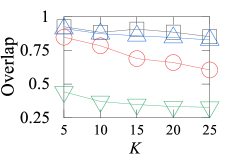
(a) $\rm IDS15K_{EN-FR}$

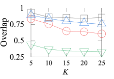
(b) $\rm IDS100K_{EN-FR}$

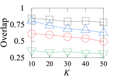
(c) $\rm DBP1M_{EN-FR}$

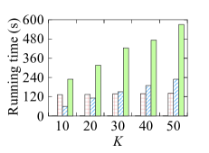
(d) $\rm DBP1M_{EN-FR}$

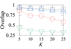
(e) $\rm IDS15K_{EN-DE}$

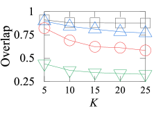
(f) $\rm IDS100K_{EN-DE}$

(g) $\rm DBP1M_{EN-DE}$

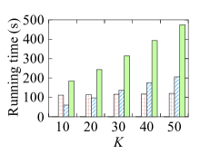
(h) $\rm DBP1M_{EN-DE}$

Figure 3. Comparison results of different batch sampling strategies

Table 3. The result of ablation study

Methods	DBP1MEN-FR			DBP1MEN-DE
	H@1	H@10	MRR	H@1	H@10	MRR
ClusterEA	28.1	47.4	0.35	28.8	48.8	0.35
ClusterEA - Sp-CSLS	27.9	46.2	0.34	28.4	46.0	0.34
ClusterEA - Global Sim	27.6	48.3	0.34	28.3	48.7	0.35
ClusterEA - Sinkhorn	20.0	46.1	0.29	22.7	46.2	0.30
ClusterEA - CMCS	26.5	46.2	0.33	26.8	47.1	0.33
ClusterEA - ISCS	25.3	45.9	0.32	25.5	46.5	0.32
ClusterEA - Dual-AMN	10.0	24.5	0.15	6.9	17.7	0.11

5.3. Ablation Study

In ablatoin study, we remove each component of ClusterEA, and report H@$1$, H@$10$, and MRR in Table 3. First, after removing the Sp-CSLS component, the accuracy of ClusterEA drops. This shows that the Sp-CSLS normalization indeed address the geometric problems of global similarity on large-scale EA. Second, after removing the global similarity, H@$1$ of ClusterEA drops but H@$10$ grows on DBP1M_EN-FR. The fluctuation on H@$10$ may be due to the incompleteness of global similarity normalization that disturbs the final similarity matrix. Specifically, the local similarity is normalized into nearly permutation matrices with Sinkhorn iteration, where most values of one row are close to zero. When fusing local and global similarity matrices, elements that are not top-1 in the local matrix will be biased towards the value of the global matrix, which is only partially normalized. This causes the disturbance. However, the incompleteness of normalization does not degrade H@$1$. This is because the value of one row in $\mathcal{M}_{L}$ that is correctly aligned will be normalized into a higher value, providing resistance to the global matrix disturbance. Third, after removing the Sinkhorn iteration, the accuracy of ClusterEA drops significantly. This confirms the importance of normalizing the similarity matrices. Finally, after removing each sampler of ClusterSampler, the accuracy of ClusterEA drops on all metrics. This validates the importance of fusing information from multi-aspects, including cross-KG information and intra-KG information. In addition, we observe that CMCS has less influence compared with ISCS. This is mainly due to the following two reasons. First, CMCS generally clusters entities with similar embedding vectors, where each batch still suffers from geometric problems. On the contrary, ISCS samples batches based on the graph neighborhood information, which is a strong constriction on the learning model. Second, we apply ISCS in both directions. In this case, it can capture more information than CMCS. By replacing its Dual-AMN model with the GCNAlign model, the accuracy of ClusterEA drops significantly on all metrics. This demonstrates the importance of the ability of the incorporated EA model in ClusterEA.

5.4. Case Study: ClusterSampler Analysis

The ClusterSampler is a vital component of ClusterEA. To ensure scalability, we set the batch number $K$ such that the space cost of the normalization process does not exceed the GPU memory. We also need to guarantee that our batch sampling method can produce acceptable mini-batches under different $K$ settings. Thus, we provide a detailed analysis on varying the batch number $K$ for different batch samplers from ClusterSampler (i.e., ISCS and CMCS). Specifically, we study how much are the mini-batches generated by one sampler acceptable as the percentage of equivalent entities that are placed into the same mini-batches (denoted as Overlap). Next, we report the Overlap metric and running time of the proposed sampler, where the mini-batch number $K$ of the proposed sampler is varied from 5 to 25 on IDS and is varied from 10 to 50 on DBP1M. We compare the proposed sampler with two rule-based baselines, VPS and METIS-CPS. VPS randomly partitions seed alignments and all other entities into different mini-batches. METIS-CPS sets the training entities with higher nodes to sample better mini-batches. Note that both METIS-CPS and ISCS are unidirectional. Thus, we apply these methods in both directions, and present their average performance of the two directions. We report the overlap of all sampling methods on all benchmarks in Fig 3, where Figures 3(a), 3(b), 3(c), 3(e),  3(f), and 3(g) are the overlap of different datasets. The results show that CMCS generally outperforms two baselines on all the datasets, and its performance is stable when varying $K$. However, although it is better overlapped, it may incur hubness and isolation problems in mini-batches (cf. Section 5.3). Thus, fusing multi-aspect is essential for ClusterEA. ISCS results in less overlapped mini-batches while still much better than METIS-CPS. This is because METIS does not necessarily follow the guidance provided by METIS-CPS. The GNN node classification model in ISCS, which considers the cross-entropy loss as a penalty, is forced to learn mini-batches more effectively. Since we set the training ratio to 30%, all samplers have an overlap over 30%, including VPS that splits mini-batches randomly. Finally, we report the running time on DBP1M in Figures 3(d) and 3(h). Since all samplers achieve sufficiently high efficiency on IDS datasets, we do not present the running time of all samplers on IDS due to space limitation. It is observed that, although the result is unacceptable, VPS is the fastest sampling method. Both the proposed ISCS and CMCS are always about $2\times$ faster than the rule-based METIS-CPS when changing $K$. The reason is that both of them utilize machine learning models that can be easily accelerated with GPU.

6. Conclusions

We present ClusterEA to align entities between large-scale knowledge graphs with stochastic training and normalized similarities. ClusterEA contains three components, including stochastic training, ClusterSampler, and SparseFusion, to perform large-scale EA task based solely on structure information. We first train a large-scale Siamese GNN for EA in a stochastic fashion to produce entity embeddings. Next, we propose a new ClusterSampler strategy for sampling highly overlapped mini-batches taking advantage of the trained embeddings. Finally, we present a SparseFusion process, which first normalizes local and global similarities and then fuses them to obtain the final similarity matrix. The whole process of ClusterEA guarantees both high accuracy and comparable scalability. Considerable experimental results on EA benchmarks with different scales demonstrate that ClusterEA significantly outperforms previous large-scale EA study. In future, it is of interest to explore dangling settings (Sun et al., 2021) of EA on large scale datasets.

7. Acknowledgements

This work was supported in part by the National Key Research and Development Program of China under Grant No. 2021YFC3300303, the NSFC under Grants No. (62025206, 61972338, and 62102351), and the Zhejiang Provincial Natural Science Foundation under Grant No. LR21F020005. Lu Chen is the corresponding author of the work.

Appendix A Normalized Hard Sample Mining Loss

We detail the NHSM loss used in our work here. Formally, for the current mini-batch, the training loss is defined as

(3) $$L=LogSumExp(\lambda z(e_{s},e_{t}))+LogSumExp(\lambda z(e_{t},e_{s}))$$

, where $e_{s}\in B_{s}$, $e_{t}\in B_{t}$, $(e_{s},e_{t})\in\phi^{\prime}$ , and $LogSumExp(X)=log(\sum_{x\in X}e^{x})$ is an operator to smoothly generate hard negative samples, $\lambda$ is the smooth factor of $LogSumExp$, and $z\in\mathcal{R}^{|B_{t}|}$ is the normalized triple loss, defined as

(4) $$z(e_{s},e_{t})=\operatorname{z-score}(\{\gamma+\operatorname{sim}(e_{s},e_{t})-\operatorname{sim}(e_{s},e_{t}^{\prime})|e^{\prime}_{t}\in B_{t}\}),$$

where $\operatorname{z-score}(X)=\frac{X-\mu(X)}{\sigma(X)}$ is the standard score normalization, and $\operatorname{sim}(e_{s},e_{t})=\mathbf{h}_{e_{s}}\cdot\mathbf{h}_{e_{t}}$ is the similarity of two entities obtained with the GNN output feature.

Appendix B Adjacency Matrix Construction for ISCS

Following (Wang et al., 2018), to construct the adjacency matrix $A\in R^{|E|\times|E|}$, we compute two metrics, which are called functionality and inverse functionality, for each relation:

(5) $$\operatorname{fun}(r)=\frac{\#Head\_Entities\_of\_r}{\#Triples\_of\_r}$$

$$\operatorname{ifun}(r)=\frac{\#Tail\_Entities\_of\_r}{\#Triples\_of\_r}$$

where $\#Triples\_of\_r$ is the number of triples of relation $r$,
$\#Head\_Entities\_of\_r$ is the number of head entities of $r$, and
$\#Tail\_Entities\_of\_r$ is the number of tail entities of $r$. To measure the influence of the $i$-th entity over the $j$-th entity, we set $a_{ij}\in A$ as:

(6) $$a_{ij}=\sum_{\left\langle e_{i},r,e_{j}\right\rangle\in G}\operatorname{ifun}(r)+\sum_{\left\langle e_{j},r,e_{i}\right\rangle\in G}\operatorname{fun}(r)$$

Appendix C Statistics of datasets

Table 4. Statistics of IDS15K, IDS100K, and DBP1M

Datasets		#Entities	#Relations	#Triples
IDS15K	EN-FR	15,000-15,000	267-210	47,334-40,864
	EN-DE	15,000-15,000	215-131	47,676-50,419
IDS100K	EN-FR	100,000-100,000	400-300	309,607-258,285
	EN-DE	100,000-100,000	381-196	335,359-336,240
DBP1M	EN-FR	1,877,793-1,365,118	603-380	7,031,172-2,997,457
	EN-DE	1,625,999-1,112,970	597-241	6,213,639-1,994,876

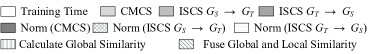
(a) EN-FR

(b) EN-DE

Figure 4. Scalability analysis vs. variants of ClusterEA

Appendix D Implementation Details

The results of all the baselines are obtained by our re-implementation with their publicly available source codes. All experiments were conducted on a personal computer with an Intel Core i9-10900K CPU, an NVIDIA GeForce RTX3090 GPU, and 128GB memory. The programs were all implemented in Python. Since the deep learning frameworks used vary on different implementations of EA models, we use the NVIDIA Nsight Systems to record the GPU memory usage of all approaches uniformly. We detail the hyper-parameters used in the experiment as follows. All the hyper-parameters are set without special instructions.

D.1. Non-scalable methods

For non-scalable methods, including GCNAlign, RREA, and Dual-AMN, we follow the parameter settings reported in their original papers (Wang et al., 2018; Mao et al., 2020b, 2021a).

D.1.1. GCNAlign

Note that GCNAlign contains an attribute encoder as the side information component. We re-implement the GCNAlign model by removing attribute features from it.

D.2. LargeEA

We reproduce LargeEA by removing entirely the name channel. It is worth noting that LargeEA incorporates a name-based data augmentation process for generating alignment seeds other than training data. For fair comparison, we also remove this augmentation process, making the LargeEA framework not use any alignment signals apart from the training data. To be more specific, we only compare the structure-channel of LargeEA. The running time and maximum GPU memory usage are also recorded only for the structure-channel of LargeEA, including METIS-CPS partitioning and mini-batch training. We use the default settings reported in (Ge et al., 2022) of the two versions, LargeEA-G and LargeEA-R. For the newly proposed variant LargeEA-D, we keep all the hyper-parameters unchanged except the structure-based EA model-related parameters switched to the default settings of Dual-AMN (Mao et al., 2021a).

D.3. Stochastic training variant of non-scalable methods

Contributed by the NHSM loss (Mao et al., 2021a), the training epoch number could be greatly reduced. We replace the training epoch for GCNAlign-S and RREA-S from 2000 and 1200 to 50. We follow (Mao et al., 2021a) to train 20 epochs for Dual-AMN-S on IDS datasets. We further notice that the training loss of Dual-AMN-S is stable after 10 epochs for the large-scale dataset DBP1M, thus setting the training epoch of Dual-AMN-S to 10 for DBP1M. We set the fan out number in neighborhood sampling $F=8$, the batch size $N_{p}=2000$, $N_{n}=4000$, and Adam as the training optimizer for all variants. We follow the setup of (Mao et al., 2021a) for NHSM loss. For other hyper-parameter settings of the model, including the embedding dimension $D$, we follow their original papers (Wang et al., 2018; Mao et al., 2020b, 2021a).

D.4. ClusterEA

In the stochastic training process, we adopt the aforementioned settings for each ClusterEA variant. In the ClusterSampler process, we set the mini-batch number $K=5$ for IDS15K, $K=10$ for IDS100K, and $K=30$ for DBP1M. Moreover, we utilize a cache in disk for pre-processed edge information to quickly load the constructed matrix of relation-aware GNN variants. For CMCS, we set the max iteration number to $300$, the tolerance to $10^{-4}$, and distance metric to euclidean distance for the KMeans algorithm. We adopt the default setting for the XGBoost Classifier (Chen and Guestrin, 2016). We utilize GPU acceleration for those methods. For ISCS, we adopt the default setting of METIS (Karypis and Kumar, 1998), and train a two layer GCN with Adam. The learning rate is set to $0.01$, and the training epoch of GCN set to $800$ for IDS15K, $1500$ for IDS100K, and $3000$ for DBP1M. In the SparseFusion process, we set $K_{s}=100$ for the iteration round of Sinkhorn, $K_{r}=50$ for top-K similarity serach, and $K_{n}=10$ for CSLS.

Appendix E Scalability Evaluation

To further investigate the scalability of our proposed ClusterEA framework, we verify the running time of each components in different variants of ClusterEA on the DBP1M dataset, including (1) Training time of the EA model; (2) CMCS batch sampling time; (3) ISCS batch sampling time on both directions; (4) Local Similarity Normalization time of the batches generated by each samplers, denoted as Norm(Sampler); (5) Calculating Global Similarity time in SparseFusion; and (6) Fusing Global and Local Similarity time in SparseFusion. The experimental results are shown in Figure 4, where G, R, and D denote ClusterEA-G, ClusterEA-R, and ClusterEA-D, respectively. As depicted in Figure 4, we observe that the running time of each component except for Training time does not exceed $10^{3}$ seconds on the large-scale dataset. This confirms the scalability of ClusterEA. Note that the training time of the Dual-AMN model is significantly less than that of other variants. This is contributed by the model design of Dual-AMN that could dramatically reduce the required training epochs.

References

- (1)
- Auer et al. (2007) Sören Auer, Christian Bizer, Georgi Kobilarov, Jens Lehmann, Richard Cyganiak, and Zachary G. Ives. 2007. DBpedia: A Nucleus for a Web of Open Data. In ISWC. 722–735.
- Azzalini et al. (2021) Fabio Azzalini, Songle Jin, Marco Renzi, and Letizia Tanca. 2021. Blocking Techniques for Entity Linkage: A Semantics-Based Approach. Data Sci. Eng. 6, 1 (2021), 20–38.
- Bordes et al. (2013) Antoine Bordes, Nicolas Usunier, Alberto García-Durán, Jason Weston, and Oksana Yakhnenko. 2013. Translating Embeddings for Modeling Multi-relational Data. In NIPS. 2787–2795.
- Cao et al. (2019) Yixin Cao, Zhiyuan Liu, Chengjiang Li, Zhiyuan Liu, Juanzi Li, and Tat-Seng Chua. 2019. Multi-Channel Graph Neural Network for Entity Alignment. In ACL. 1452–1461.
- Chen et al. (2021) Muhao Chen, Weijia Shi, Ben Zhou, and Dan Roth. 2021. Cross-lingual entity alignment with incidental supervision. (2021), 645–658.
- Chen et al. (2017) Muhao Chen, Yingtao Tian, Mohan Yang, and Carlo Zaniolo. 2017. Multilingual Knowledge Graph Embeddings for Cross-lingual Knowledge Alignment. In IJCAI. 1511–1517.
- Chen and Guestrin (2016) Tianqi Chen and Carlos Guestrin. 2016. XGBoost: A Scalable Tree Boosting System. In KDD. 785–794.
- Chiang et al. (2019) Wei-Lin Chiang, Xuanqing Liu, Si Si, Yang Li, Samy Bengio, and Cho-Jui Hsieh. 2019. Cluster-GCN: An Efficient Algorithm for Training Deep and Large Graph Convolutional Networks. In KDD. 257–266.
- Cuturi (2013) Marco Cuturi. 2013. Sinkhorn Distances: Lightspeed Computation of Optimal Transport. In NIPS. 2292–2300.
- Fey et al. (2020) Matthias Fey, Jan Eric Lenssen, Christopher Morris, Jonathan Masci, and Nils M. Kriege. 2020. Deep Graph Matching Consensus. In ICLR.
- Ge et al. (2021) Congcong Ge, Xiaoze Liu, Lu Chen, Baihua Zheng, and Yunjun Gao. 2021. Make It Easy: An Effective End-to-End Entity Alignment Framework. In SIGIR. 777–786.
- Ge et al. (2022) Congcong Ge, Xiaoze Liu, Lu Chen, Baihua Zheng, and Yunjun Gao. 2022. LargeEA: Aligning Entities for Large-scale Knowledge Graphs. PVLDB 15, 2 (2022), 237–245.
- Guo et al. (2019) Lingbing Guo, Zequn Sun, and Wei Hu. 2019. Learning to Exploit Long-term Relational Dependencies in Knowledge Graphs. In ICML. 2505–2514.
- Hamilton et al. (2017) William L Hamilton, Rex Ying, and Jure Leskovec. 2017. Inductive representation learning on large graphs. In NIPS. 1025–1035.
- Harold W. Kuhn (1955) Harold W. Kuhn. 1955. The Hungarian method for the assignment problem. Naval Research Logistics Quarterly 2, 1, 83–97.
- Johnson et al. (2017) Jeff Johnson, Matthijs Douze, and Hervé Jégou. 2017. Billion-scale similarity search with GPUs. arXiv preprint arXiv:1702.08734 (2017).
- Karypis and Kumar (1998) George Karypis and Vipin Kumar. 1998. A Fast and High Quality Multilevel Scheme for Partitioning Irregular Graphs. SIAM J. Sci. Comput. 20, 1 (1998), 359–392.
- Kipf and Welling (2017) Thomas N. Kipf and Max Welling. 2017. Semi-Supervised Classification with Graph Convolutional Networks. In ICLR.
- Lample et al. (2018) Guillaume Lample, Alexis Conneau, Marc’Aurelio Ranzato, Ludovic Denoyer, and Hervé Jégou. 2018. Word translation without parallel data. In ICLR.
- Li et al. (2019) Chengjiang Li, Yixin Cao, Lei Hou, Jiaxin Shi, Juanzi Li, and Tat-Seng Chua. 2019. Semi-supervised Entity Alignment via Joint Knowledge Embedding Model and Cross-graph Model. In EMNLP. 2723–2732.
- Liu et al. (2020b) Fangyu Liu, Muhao Chen, Dan Roth, and Nigel Collier. 2020b. Visual Pivoting for (Unsupervised) Entity Alignment. arXiv preprint arXiv:2009.13603 (2020).
- Liu et al. (2020a) Zhiyuan Liu, Yixin Cao, Liangming Pan, Juanzi Li, and Tat-Seng Chua. 2020a. Exploring and Evaluating Attributes, Values, and Structures for Entity Alignment. In EMNLP. 6355–6364.
- Mao et al. (2021a) Xin Mao, Wenting Wang, Yuanbin Wu, and Man Lan. 2021a. Boosting the Speed of Entity Alignment 10: Dual Attention Matching Network with Normalized Hard Sample Mining. In WWW. 821–832.
- Mao et al. (2021b) Xin Mao, Wenting Wang, Yuanbin Wu, and Man Lan. 2021b. From Alignment to Assignment: Frustratingly Simple Unsupervised Entity Alignment. In EMNLP. 2843–2853.
- Mao et al. (2020a) Xin Mao, Wenting Wang, Huimin Xu, Man Lan, and Yuanbin Wu. 2020a. MRAEA: An Efficient and Robust Entity Alignment Approach for Cross-lingual Knowledge Graph. In WSDM. 420–428.
- Mao et al. (2020b) Xin Mao, Wenting Wang, Huimin Xu, Yuanbin Wu, and Man Lan. 2020b. Relational Reflection Entity Alignment. In CIKM. 1095–1104.
- Roth (2008) Alvin E Roth. 2008. Deferred acceptance algorithms: History, theory, practice, and open questions. international Journal of game Theory 36, 3 (2008), 537–569.
- Sun et al. (2021) Zequn Sun, Muhao Chen, and Wei Hu. 2021. Knowing the No-match: Entity Alignment with Dangling Cases. In ACL. 3582–3593.
- Sun et al. (2020a) Zequn Sun, Muhao Chen, Wei Hu, Chengming Wang, Jian Dai, and Wei Zhang. 2020a. Knowledge Association with Hyperbolic Knowledge Graph Embeddings. In EMNLP. 5704–5716.
- Sun et al. (2017) Zequn Sun, Wei Hu, and Chengkai Li. 2017. Cross-Lingual Entity Alignment via Joint Attribute-Preserving Embedding. In ISWC. 628–644.
- Sun et al. (2018) Zequn Sun, Wei Hu, Qingheng Zhang, and Yuzhong Qu. 2018. Bootstrapping Entity Alignment with Knowledge Graph Embedding. In IJCAI. 4396–4402.
- Sun et al. (2019) Zequn Sun, JiaCheng Huang, Wei Hu, Muhao Chen, Lingbing Guo, and Yuzhong Qu. 2019. TransEdge: Translating Relation-Contextualized Embeddings for Knowledge Graphs. In ISWC. 612–629.
- Sun et al. (2020b) Zequn Sun, Chengming Wang, Wei Hu, Muhao Chen, Jian Dai, Wei Zhang, and Yuzhong Qu. 2020b. Knowledge Graph Alignment Network with Gated Multi-Hop Neighborhood Aggregation. In AAAI. 222–229.
- Sun et al. (2020c) Zequn Sun, Qingheng Zhang, Wei Hu, Chengming Wang, Muhao Chen, Farahnaz Akrami, and Chengkai Li. 2020c. A Benchmarking Study of Embedding-based Entity Alignment for Knowledge Graphs. PVLDB 13, 11 (2020), 2326–2340.
- Tang et al. (2020) Xiaobin Tang, Jing Zhang, Bo Chen, Yang Yang, Hong Chen, and Cuiping Li. 2020. BERT-INT: A BERT-based Interaction Model For Knowledge Graph Alignment. In IJCAI. 3174–3180.
- Velickovic et al. (2018) Petar Velickovic, Guillem Cucurull, Arantxa Casanova, Adriana Romero, Pietro Liò, and Yoshua Bengio. 2018. Graph Attention Networks. In ICLR.
- Wang et al. (2018) Zhichun Wang, Qingsong Lv, Xiaohan Lan, and Yu Zhang. 2018. Cross-lingual Knowledge Graph Alignment via Graph Convolutional Networks. In EMNLP. 349–357.
- Wang et al. (2020) Zhichun Wang, Jinjian Yang, and Xiaoju Ye. 2020. Knowledge Graph Alignment with Entity-Pair Embedding. In EMNLP. 1672–1680.
- Xiong et al. (2017) Chenyan Xiong, Russell Power, and Jamie Callan. 2017. Explicit Semantic Ranking for Academic Search via Knowledge Graph Embedding. In WWW. 1271–1279.
- Yang et al. (2020) Kai Yang, Shaoqin Liu, Junfeng Zhao, Yasha Wang, and Bing Xie. 2020. COTSAE: CO-Training of Structure and Attribute Embeddings for Entity Alignment. In AAAI. 3025–3032.
- Zeng et al. (2020a) Weixin Zeng, Xiang Zhao, Jiuyang Tang, and Xuemin Lin. 2020a. Collective Entity Alignment via Adaptive Features. In ICDE. 1870–1873.
- Zeng et al. (2021) Weixin Zeng, Xiang Zhao, Jiuyang Tang, Xuemin Lin, and Paul Groth. 2021. Reinforcement Learning-based Collective Entity Alignment with Adaptive Features. TOIS 39, 3 (2021), 26:1–26:31.
- Zeng et al. (2020b) Weixin Zeng, Xiang Zhao, Wei Wang, Jiuyang Tang, and Zhen Tan. 2020b. Degree-Aware Alignment for Entities in Tail. In SIGIR. 811–820.
- Zhang et al. (2016) Fuzheng Zhang, Nicholas Jing Yuan, Defu Lian, Xing Xie, and Wei-Ying Ma. 2016. Collaborative Knowledge Base Embedding for Recommender Systems. In KDD. 353–362.
- Zhang et al. (2019) Qingheng Zhang, Zequn Sun, Wei Hu, Muhao Chen, Lingbing Guo, and Yuzhong Qu. 2019. Multi-view Knowledge Graph Embedding for Entity Alignment. In IJCAI. 5429–5435.
- Zhao et al. (2022) Xiang Zhao, Weixin Zeng, Jiuyang Tang, Xinyi Li, Minnan Luo, and Qinghua Zheng. 2022. Toward Entity Alignment in the Open World: An Unsupervised Approach with Confidence Modeling. Data Sci. Eng. 7, 1 (2022), 16–29.
- Zhu et al. (2017) Hao Zhu, Ruobing Xie, Zhiyuan Liu, and Maosong Sun. 2017. Iterative Entity Alignment via Joint Knowledge Embeddings. In IJCAI. 4258–4264.