Physics Informed LSTM Network for Flexibility Identification in Evaporative Cooling Systems

Abstract

In energy intensive industrial systems, an evaporative cooling process may introduce operational flexibility. Such flexibility refers to a system’s ability to deviate from its scheduled energy consumption. Identifying the flexibility, and therefore, designing control that ensures efficient and reliable operation presents a great challenge due to the inherently complex dynamics of industrial systems. Recently, machine learning models have attracted attention for identifying flexibility, due to their ability to model complex nonlinear behavior. This research presents machine learning based methods that integrate system dynamics into the machine learning models (e.g., Neural Networks) for better adherence to physical constraints. We define and evaluate physics informed long-short term memory networks (PhyLSTM) and physics informed neural networks (PhyNN) for the identification of flexibility in the evaporative cooling process. These physics informed networks approximate the time-dependent relationship between control input and system response while enforcing the dynamics of the process in the neural network architecture. Our proposed PhyLSTM provides less than 2% system response estimation error, converges in less than half iterations compared to a baseline Neural Network (NN), and accurately estimates the defined flexibility metrics. We include a detailed analysis of the impact of training data size on the performance and optimization of our proposed models.

I Introduction

ENERGY intensive processes require effective control design for reliable and efficient operation [1]. An Evaporative Cooling System (ECS) is one such energy intensive process where control can be used to mitigate energy fluctuations. Designing control for ECS requires modeling the complex behavior of a non-linear system to identify its operational flexibility.

Operational flexibility of a system is the ability to deviate from the original planning in terms of energy consumption. Quantification and measurement of operational flexibility remain challenging, both theoretically and practically. This is performed using system identification, which results in parametric models with the capability of predicting the effect of control settings on the systems’ dynamic behavior [2]. System identification in energy intensive systems is thus an essential step that assists in estimating operational flexibility, developing control, making pricing/cost decisions, etc.

Traditional system identification procedures rely on a mathematical, structured model that defines the relationship between system parameters and variables. When considering dynamic physical systems, state-space models in the form of ordinary differential equations (ODEs) offer a mathematical formulation to establish this relationship [3]. Such dynamic system models are often referred to as white-box models. White-box models help control engineers to make sure an industrial process is controlled optimally. However, the limited set of parameters in white-box models fail to fully align with real-world processes.

Recently, data-driven machine learning (ML) based approaches have attracted attention for analyzing or understanding complex processes. ML based system identification has been used to build black-box models that define the relationship between control inputs and unknown parameters [4]. Such black-box models, however, lack the physical understanding of the system and can result in outputs that are physically improbable when the models fail to generalize well. To overcome this, grey-box ML based methods have been used in recent years, where the process dynamics are integrated with the data-driven approach [5].

Our objective in this paper is to present grey-box neural networks that are physics-informed, i.e., which adhere to prior physical knowledge. We particularly present a methodology for neural networks to follow a first order differential equation that describes the physical process. As an exemplary use case, we focus on an induced draft cooling tower [6]. Specifically, we devise and evaluate two state-of-the-art grey-box models, applied to the induced draft cooling tower: physics informed neural networks (PhyNN) and physics informed long-short term memory networks (PhyLSTM). These models enforce the system’s dynamics onto the neural network, in contrast to a black-box neural network (NN) model that follows a free structure. PhyLSTM is based on a recurrent neural network (RNN) architecture. RNNs are types of artificial neural networks that use the output of previous steps as inputs of the current step. Such architecture helps to learn the sequential dependencies and is beneficial for time-dependent modeling. Furthermore, we define a formulation to estimate operational flexibility based on system response from these identified models.

Our main contributions in this paper are, that we (i) devise the architecture for two novel data-driven grey-box modeling approaches, based on physics informed networks, i.e., PhyNN and PhyLSTM (Section IV), (ii) extend the white-box model for an ECS to calculate operational flexibility based on two proposed metrics (Section III), and (iii) compare the accuracy and evaluation time of physics informed networks (PhyNN and PhyLSTM) with those of both white-box as well as black-box (e.g., neural network NN) models. For the performance comparison, we simulate data from a white-box model (Section V) and train the data-driven models based on designed experiments to evaluate the potential of data-driven grey-box models for system identification and address the following questions (Section VI):

1. How do the grey-box models perform compared to the black-box and white-box models, in terms of accuracy?

2. Does using a recurrent neural network architecture decrease the estimation error of the grey-box models (PhyLSTM compared to PhyNN)?

3. What is the impact of amount of training data on (i) the estimation error, (ii) the optimization, and (iii) the training and evaluation time of the data-driven models?

4. What is the estimated operational flexibility in ECS using data-driven models?

Section VII summarizes conclusions and open issues that can be addressed in future work. We note that the specific models and corresponding numerical performance results are for the selected representative use case of the evaporative cooling system, but the methodology followed to construct these models is applicable in general to various processes that can be approximated as a first order differential equation.

II Related work

II-A Machine learning in System Identification

System identification in energy-intensive industrial processes such as an evaporative cooling system (ECS) is a crucial step for control design, fault detection, flexibility exploitation, etc. Traditionally, white-box models are used for system identification. For example, a mathematical model for simulation of refinery furnaces is proposed in [7]. The furnace model quantifies the main control variables for refinery services by combining a process model and a flue gas side model. A model-based system identification for fault detection in a gas turbine is proposed in [8], which identifies ‘residuals’ that are the errors in the measured and estimated variables of the process. As opposed to identification for fault detection or forecasting, we rather focus on identifying system output that can be exploited to build effective control for an energy-intensive industrial process (i.e., by identifying system parameters that provide operational flexibility).

In contrast to [8], which uses white-box models for system identification, multiple data-driven black-box models are proposed in [9] to predict the parameters of an energy-intensive thermal stabilization process in carbon fiber production. A black-box long-short term memory (LSTM) recurrent NN in [10] provides accurate predictions of power fluctuations compared to real-time measurements. In our work, we focus on data-driven grey-box models, which are superior to the black-box models, as they include the process dynamics in the modeling approach and thus better adhere to physical constraints of the system (i.e., by avoiding physically improbable outputs).

Grey-box machine learning models have been studied in the past. For example, [11] proposed a physics-informed neural network architecture that learns the system’s output while respecting its physical laws (described using ODE/PDE). They evaluated these networks on systems described by the Schrodinger equation, the Navier–Stokes equation, etc. A grey-box model based on neural networks that respect Lagrangian mechanics is proposed in [12]. Our work is different from these works in two aspects: (i) unlike [11] and [12], we evaluate the grey-box models for a energy-intensive ECS, and (ii) we propose a newly designed LSTM-based recurrent neural network architecture for the grey-box modeling . We evaluate our grey-box models for system identification in an induced draft cooling tower that is a part of an ECS.

II-B Evaporative Cooling System (ECS)

An induced draft cooling tower is an essential part of the overall ECS that provides opportunities to build effective control. A white-box model for the induced draft cooling tower based on first principles is proposed in [6]. A comparison of this white-box model and a black-box model based on an adaptive neuro-fuzzy interference system (i.e., a neural network trained with an interference system based on fuzzy rules) in [13] shows that white-box models are superior for identifying basin temperature in the induced draft cooling tower. However, white-box models are computationally expensive and challenging to implement in a real-world setup. In this paper, we aim to overcome these challenges by defining grey-box physics informed networks (PhyNN and PhyLSTM) that (i) are computationally less expensive than the white-box models defined in [6], and (ii) respect the physical laws of the system, as opposed to the model defined in [13] .

Since flexibility is an abstract term, its quantification is a difficult task. Approaches towards quantifying and exploiting operational flexibility follow simple methodologies. For example, in [14] technical flexibility constraints are estimated individually in energy-intensive processes, while ignoring their internal dependencies. Quantifiable features of demand-side flexibility (e.g., time frame, storage capacity, interdependent jobs etc) are identified in [15]. As opposed to using such a broad range of demand side parameters, we define operational flexibility using just two metrics, namely, state of charge and rate of charge, which represent the flexible characteristics of the system response (See further, Section III-B).

III Induced Draft Cooling tower

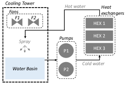
Fig. 1: Simplified diagram of a evaporative cooling system

An induced draft cooling tower is a part of the ECS. A typical ECS comprises fans and cooling water pumps, which are the primary energy consumers, as well as pipes, valves, and heat exchangers (HEXs). Figure 1 shows the simplified version of the considered ECS, where the water is circulated and pumped using pumps to the set of HEXs. They cool down the process in a closed-circuit. The cooling tower consists of fans, a hot water spray, and a water basin.

The physical state change from a fluid (water) to a gas (water vapor) requires latent heat. This heat is extracted from the water, resulting in a temperature decrease. This physical phenomenon is exploited within the cooling process by spraying warm water in a cooling tower, where fans induce a counter airflow to maximize the air-water interaction. As a result, the water falling in the basin underneath has dropped in temperature and can be recirculated through the process. Together with the heat evacuation, also mass leaves the system in the form of water vapor.

During this process, the basin temperature should remain within a specified range. It can be controlled using the control inputs (fan powers) and can be employed to calculate the process’s operational flexibility. We will estimate the operational flexibility by simulating and predicting the water basin temperature response to fan power changes. Different methods can be adopted to model the basin temperature based on the fans’ power, including mathematical models and data-driven models. In this section, a white-box model of the induced draft cooling tower based on previous research [13] is extended to estimate the operational flexibility of the process.

III-A White-box model

A white-box thermodynamic model of the cooling tower system is developed based on the laws of heat transfer and mass conservation [13]. This model is presented in Eq. (1), where $T_{b}$ is the basin temperature. This model is defined using the process heat $Q_{p}$ [W], the cooling capacity $Q_{t}$ [W], the specific heat capacity of water $c_{w}$ [kJ/kg·k], the water volume $V_{w}$ [m³] and the water density $\rho_{w}$ [kg/m³].

$$\frac{\partial T_{b}}{\partial t}=\frac{Q_{p}-Q_{t}}{c_{w}\cdot V_{w}\cdot\rho_{w}}$$ (1)

The process heat $Q_{p}$ is expressed as in Eq. (2), where $\dot{m}_{w}$ is the mass flow of water [Kg/s], $T_{p}$ is the process water temperature [K] and $T_{b}$ is the water basin temperature [K]. Note that the $\dot{m}_{w}$, i.e., mass flow of process water, depends on the industrial process.

$$Q_{p}=\dot{m}_{w}\cdot c_{w}\cdot(T_{p}-T_{b})$$ (2)

The cooling capacity $Q_{t}$ is expressed as in Eq. (3), where $\dot{m}_{a}$ is the mass flow of air [Kg/s], $H_{a,e}$ and $H_{a,l}$ are the entering and leaving air enthalpy [kJ/kg·K], respectively.

$$Q_{t}=\dot{m}_{a}\cdot(H_{a,e}-H_{a,l})$$ (3)

Enthalpies can be calculated using humidity rates and temperature [16]. The entering air enthalpy depends on the ambient air temperature, and the leaving air enthalpy depends on the leaving air temperature. The mass flow rate of air depends on the power supplied to the fans and is expressed in Eq. (4).

$$\dot{m}_{a}=\sqrt{\frac{2\cdot P_{f}\cdot\rho_{a}\cdot A^{2}_{\text{fr}}\cdot\eta_{\text{fan}}\cdot\eta_{\text{motor}}}{6.5+K_{el}+2\cdot\frac{A^{2}_{\text{fr}}}{A^{2}_{\text{fan}}}}}$$ (4)

where $P_{f}$ is the electric fan power [W], $A_{\text{fr}}$ is the tower frontal area [m²], $A_{\text{fan}}$ is the fan area [m²], $\eta_{\text{fan}}$ is the fan efficiency [%], $\eta_{\text{motor}}$ is the motor efficiency [%] and $K_{el}$ is the eliminator coefficient (if unknown, it is set to 1). The air density is represented by $\rho_{a}$ and is calculated for the mixture of dry air and water vapor. In a cooling tower, reliable operation is ensured if the basin temperature is within a range defined using the minimum and maximum operational requirements (Eq. (5)). Operational flexibility offered by the cooling tower based on the range of $T_{b}$ is defined next.

$$T_{b,\text{min}}\leq T_{b}\leq T_{b,\text{max}}$$ (5)

III-B Operational Flexibility

To quantify operational flexibility, we adopt the framework of Ulbig and Andersson [17], who represent the system as a virtual battery. This virtual battery is defined by representing the process in the form of a power node [18]. The advantage of this approach is that it is independent of system configurations (e.g., the number of fans), and can generalize to any system represented as a virtual battery.

To quantify the operational flexibility in an evaporative cooling tower, we represent it as a thermal battery, where power is fed into the process through the fans that feed air into the tower. The operational flexibility of this thermal battery is given by two metrics, namely, (i) State of Charge ($SoC$), and, (ii) Rate of Charge ($RoC$). The $SoC$ represents the flexibility characterized by the state of operation, and is calculated using the basin temperature $T_{b}$. The $SoC$ is defined in Eq. (6) where $1/\eta$ is the efficiency. The range of $SoC$ is from 0 to $(T_{b,\text{max}}-T_{b,\text{min}})/{\eta}$. The $RoC$ represents the flexibility offered charging/discharging, i.e., the transition speed between states of operation. $RoC$ is defined in Eq. (7)

$$SoC={(T_{b}-T_{b,\text{min}})}/\eta$$ (6)

$$RoC=\frac{1}{\eta}\frac{\partial T_{b}}{\partial t}$$ (7)

Compared to [17], we thus define new operational flexibility metrics, i.e., $SoC$ and $RoC$, that are used specifically for energy intensive industrial processes such as the exemplary induced draft cooling tower. For the cooling tower, $SoC$ provides the nominal cooling production capacity and $RoC$ provides the cooling capacity variation relative to the power consumption.

IV Data-Driven Models

Data-driven models offer an alternative to white-box dynamic models (Section III-A) to construct behavioral input-output models. Data-driven models are faster to evaluate compared to white-box models. A data-driven model is also efficient in terms of space complexity and can be saved and evaluated in real-time. These models can be trained on either real-world data or simulated data. This section presents typical architectures for the black-box (Section IV-A) and grey-box (Section IV-B) data-driven models that are employed to approximate the time-varying relationship between the control inputs and system responses, specifically for the considered ECS. Section IV-C summarizes the loss functions used to train the models. Finally, Section IV-D presents how the operational flexibility is estimated using the data-driven models.

IV-A Black-box models

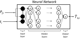
Fig. 2: Black-box NN (Not all connections between cells are shown to keep the figure legible)

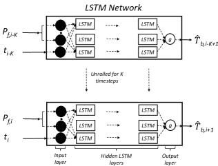
Fig. 3: Black-box LSTM unrolled in time for K timesteps (Not all connections between cells are shown to keep the figure legible)

To approximate the evaporative cooling system, we consider two black-box models: (i) a typical Neural Network (NN), and (ii) a typical Long short-term memory network (LSTM). Both black-box models designed with the control input being the fan power $P_{f}$ and system response basin temperatures $T_{b}$. The basin temperature depends on the time of day (since ambient air temperature and its pressure change during the day). Thus we include the timeslot (t) as model inputs, providing a temporal component to the model. The approximated basin temperature $\widehat{T}^{\textit{NN}}_{b}$ is obtained from a neural network (NN) with weights $\theta$, as stated by Eq. (8). The timeslot $t_{i}$ represents the time of day. For example, if the timeslot duration ($\Delta t$) is 15 minutes, a 24 hour day will have 96 timeslots, i.e., t_i $\in\{1,2,\dots,96\}$.

$$\widehat{T}^{\textit{NN}}_{b,i}=\textit{NN}({P_{f,i},t_{i};\theta})$$ (8)

Figure 2 provides the architecture of the mentioned NN model, where i represents the $i^{th}$ observation. The activation function for each cell is represented by g and can be chosen depending on the problem (e.g., sigmoid, softmax, ReLu, etc.)

An LSTM network is a type of recurrent neural network where each layer has LSTM cells characterized by a state that is updated based on the previous timestep state and current input, controlled through so-called forget gate, input gate and output gate [19]. This network is used for temporal or sequential modeling, where the outputs of a step depend on the output of previous steps. The approximated basin temperature $\widehat{T}^{\textit{LSTM}}_{b}$ at timestep $t_{i}$ thus depends on the control inputs of previous $K$ timesteps (Eq. (9)). To estimate the basin temperate at the $i^{th}$ timestep, we sequentially feed the control inputs from timestep $i-K$ to timestep $i$. The sequence length (K) depends on the problem and can be chosen based on the past dependencies of the output. Figure 3 provides the architecture of the mentioned LSTM model where we feed data for $K$ timesteps and get the final output basin temperature for the $i$+1${}^{\textrm{th}}$ timestep.

$$\widehat{T}^{\textit{LSTM}}_{b,i}=\textit{LSTM}({P_{f,i},t_{i},\dots,P_{f,i-K},t_{i-K};\theta})$$ (9)

IV-B Grey-box models

A grey-box model combines data-driven with physics-based models to improve the reliability of the model. Physics informed networks are used as grey-box models to approximate the behavior of a dynamic system. An induced draft cooling tower is characterized by Eq. (1), where $T_{b}$ is the system response which is approximated using a neural network. Raissi et al. [11] suggest to define a function $f$ by rewriting Eq. (1) as in Eq. (10), thus allowing us to evaluate the adherence of the grey-box model to the system dynamics by utilizing $\widehat{f}$, as the approximation of ${f}$. The second term of this is defined as operator $H$ in Eq. (11), characterized by parameters $\beta$, which represents the parameters used in the calculation of $Q_{p}$ and $Q_{t}$. In our case of a cooling tower, $\beta$ includes constants such as specific enthalpy, density, the universal gas constant, etc. We can calculate $Q_{p}$, using Eq. (2), based on $T_{b}$ and $\beta$. Similarly, $Q_{t}$ can be calculated with Eq. (3) and Eq. (4) using $T_{b}$, $\beta$ and $W$ (a tuple constructed from temperature, pressure, and humidity of ambient air).

$$f\triangleq\frac{\partial T_{b}}{\partial t}-\frac{Q_{p}-Q_{t}}{c_{w}\cdot V_{w}\cdot\rho_{w}}$$ (10)

$$H(T_{b},W;\beta)=\frac{Q_{p}-Q_{t}}{c_{w}\cdot V_{w}\cdot\rho_{w}}$$ (11)

IV-B1 Physics Informed Neural Networks (PhyNN)

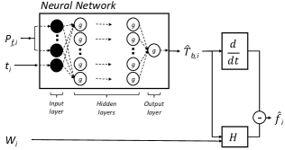
Fig. 4: Grey-box PhyNN (Not all connections between cells are shown to keep the figure legible).

Dynamics of the cooling tower can be enforced on the neural network architecture using Eq. (10). In Fig. 4 we illustrate the PhyNN architecture, where i is the $i^{th}$ observation. A neural network is used to approximate the basin temperature (Eq. (12)). The time derivative of the basin temperature is determined using auto differentiation. The function $\widehat{f}^{\textit{PhyNN}}$ is estimated using $\widehat{T}^{\textit{PhyNN}}_{b}$ and the weather data (W: Temperature, pressure and humidity) for each timestep, Eq. (13).

$$\widehat{T}^{\textit{PhyNN}}_{b,i}=\textit{PhyNN}({P_{f,i},\textit{t}_{i};\theta})$$ (12)

$$\widehat{f}^{\textit{PhyNN}}_{i}=\left(\frac{\partial\widehat{T}^{\textit{PhyNN}}_{b}}{\partial t}\right)_{i}-H(\widehat{T}^{\textit{PhyNN}}_{b,i},W_{i};\beta)$$ (13)

IV-B2 Physics Informed LSTM Networks (PhyLSTM)

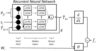
Fig. 5: Grey-box $\text{PhyLSTM}_{\textit{WF}}$. The physics informed LSTM network with feedback from output to inputs of the LSTM network. (Not all connections between cells are shown to keep the figure legible).

The PhyLSTM model is designed to enforce the physics of the cooling tower on a typical LSTM network at each timestep $i$. The approximated value of basin temperature parameter $f$ at step $i$ is calculated using Eq. (14) and Eq. (15).

$$\widehat{T}^{\textit{PhyLSTM}}_{b,i}=\textit{PhyLSTM}({P_{f,i},t_{i},\dots,P_{f,i-K},t_{i-K};\theta})$$ (14)

$$\widehat{f}^{\textit{PhyLSTM}}_{i}=\left(\frac{\partial\widehat{T}^{\textit{PhyLSTM}}_{b}}{\partial t}\right)_{i}-H(\widehat{T}^{\textit{PhyLSTM}}_{b,i},W_{i};\beta)$$ (15)

Similar to the PhyNN, the time derivative is calculated using auto differentiation and $H$ is calculated using the weather data (${W_{i}}$) and the output of the network ($\widehat{T}^{\textit{PhyLSTM}}_{b,i}$).

LSTM is a widely known RNN architecture for time series modeling which updates weights by error propagation through time using LSTM cell states. The LSTM cell architecture consists of connections (known as gates) that manipulate inputs, e.g., $P_{f}$, to estimate the output, e.g., $T_{b}$, and update the cell state in each recurrent step [19]. This updated cell state feedback is further used in the next recurrent timestep. NARX models offer an alternative way of time series modeling, through using direct feedback of the output. As opposed to a linear chain of LSTM cells, a NARX model uses a simple feed-forward network to estimate outputs [20]. A NARX uses direct feedback connections: the output of the past timestep is fed as input of the current timestep, but without having other state feedback (cf. the hidden state of an LSTM cell). The output feedback in these models has proven its effectiveness in accurate long-term time series modeling [21]. In PhyLSTM, physics is enforced on the output $T_{b}$ estimated by the LSTM network, where LSTM cell states are propagated through time. We note that the basin temperature ($T_{b}$) of the current timestep depends on its past values. Thus, to fully explore the potential of PhyLSTMs, in addition to cell state feedback, we introduce output feedback for time series modeling of $T_{b}$.

We design two PhyLSTM architectures based on the feedback from the output of the network to its input. More specifically, (i) an architecture with feedback $\text{PhyLSTM}_{\textit{WF}}$, where to estimate $\widehat{T}^{\textit{PhyLSTM}}_{b}$ at $i^{th}$ timestep, the estimated basin temperature of $(i-1)^{th}$ timestep is fed as input to the LSTM network, and (ii) an architecture without feedback $\text{PhyLSTM}_{\textit{WOF}}$. Figure 5 describes the architecture of $\text{PhyLSTM}_{\textit{WF}}$, with the feedback of previous basin temperature for a single timestep. During training, we unroll the network for $K$ timesteps similar to the black-box LSTM network Fig. 3. In case of $\text{PhyLSTM}_{\textit{WOF}}$, the output feedback connection in the LSTM network is removed.

IV-C Training and Loss Functions

For the black-box NN and LSTM models, the weights ($\theta$) of the networks are optimized by minimizing the loss function defined using mean squared error (MSE) in estimating the basin temperature $T_{b}$. For example, Eq. (16) provides this loss function for NN, where the approximated value of basin temperature $T_{b,i}$ is represented by $\widehat{T}^{N\!N}_{b,i}$. The total number of observations in a batch is represented by B. The second term in Eq. (16) is $\mathcal{L}2$ regularization, which prevents the network’s weights from increasing excessively. The hyper-parameter $\lambda$ controls the importance of the regularization term.

$$\mathcal{L}^{\textit{NN}}(\theta) =\frac{1}{B}\sum\limits_{i=1}^{B}(T_{b,i}-\hat{T}^{\textit{NN}}_{b,i})^{2}+\frac{\lambda}{B}\sum\limits_{i=1}^{B}|\theta_{i}|^{2}$$ (16)

$$\mathcal{L}^{\textit{PhyNN}}(\theta)= \frac{1}{B}\sum\limits_{i=1}^{B}\Biggl{\{}\left(T_{b,i}-\widehat{T}^{\textit{PhyNN}}_{b,i}\right)^{2}+\left(\widehat{f}^{\textit{PhyNN}}_{i}\right)^{2}\Biggr{\}}$$

$$+\frac{\lambda}{B}\sum\limits_{i=1}^{B}|\theta_{i}|^{2}$$ (17)

Loss functions used to train the neural networks in grey-box models are based on the error in estimating $T_{b}$: ($T_{b,i}~{}-~{}\widehat{T}^{\textit{PhyNN}}_{b,i}$), and the error in enforcing system dynamics, i.e., $f$: ($f_{i}~{}-~{}\widehat{f}^{\textit{PhyNN}}_{i}$). We train the networks by minimizing the total mean squared error (MSE), i.e., summing the MSEs of $T_{b}$ and $f$ [11]. Adding the MSE of $f$ ensures that the neural network maximally adheres to the dynamic system’s physics. In Eq. (17), we give the loss function for PhyNN based on weights $\theta$. Estimated values of $T_{b}$ and $f$ for the $i^{th}$ observation are represented by $\widehat{T}^{\textit{PhyNN}}_{b,i}$ and $\widehat{f}^{P\!h\!y\!N\!N}_{i}$ respectively. The last term is $\mathcal{L}2$ regularization. The equation is simplified based on the true value of $f_{i}$ = 0 (Eq. (10)).

While training the PhyLSTM, we pass $K$ sequential inputs through the network. The full set of observations in a batch ($B$) are divided into $C$ parts, where each part comprises $K$ sequential inputs. The total number of such parts is given by $C$ = $\lfloor B/K\rfloor$. Thus, the total number of observations used to train PhyLSTM is CK. Eq. (18) provides the loss function for the PhyLSTM model, where mean square errors are calculated for all parts and all timesteps. $\mathcal{L}2$ regularization is specifically useful to avoid overfitting an LSTM network trained using ‘teacher-forcing’.

$$\quad\mathcal{L} {}^{\textit{PhyLSTM}}(\theta)=$$

$$\frac{1}{CK}\sum\limits_{c=1}^{C}\sum\limits_{k=1}^{K}\Biggl{\{}\left(T_{b,k}-\widehat{T}^{\textit{PhyLSTM}}_{b,k}\right)^{2}+\left(\widehat{f}^{\textit{PhyLSTM}}_{k}\right)^{2}\Biggr{\}}_{c}$$

$$+\frac{\lambda}{CK}\sum\limits_{i=1}^{CK}|\theta_{i}|^{2}$$ (18)

Algorithm 1 Training PhyNN and PhyLSTM

0:  $\mathcal{D}$ = $\{(P_{f},t,W)_{i}$,$~{}(T_{b})_{i}\}_{i=1}^{B}$

0:  $\mathcal{M}$ (Trained model)

1:  $\mathcal{M}$ = Model $\in\{\textit{PhyNN},\textit{PhyLSTM\}}$;

2:  $\theta$ = weights of the network in $\mathcal{M}$;

3:  while not stopping condition do

4:     for all i do

5:        $\widehat{T_{b}}$ = $\mathcal{M}$($P_{f},t;\theta$);

6:        $\widehat{f}$ = $\mathcal{M}$($P_{f},t,W;\theta$);

7:        $\theta\leftarrow\theta-\alpha\frac{dL^{\mathcal{M}}(\theta)}{d\theta}$; {Update weights using $\widehat{T_{b}}$ and $\widehat{f}$}

8:     end for

9:  end while

10:  return  $\mathcal{M}$

Pseudocode for training the physics informed networks is provided in Algorithm 1, where we represent a physics informed network by $\mathcal{M}\in\{PhyNN,PhyLSTM\}$. The loss $\mathcal{L}^{\mathcal{M}}(\theta)$ is given by Eq. (17) or Eq. (18), based on the chosen model $\mathcal{M}$.

IV-D Operational Flexibility Identification

Using the physics informed networks, we can get the estimated values of the basin temperature $\widehat{T}_{b}$ and its derivative $\frac{\widehat{dT_{b}}}{dt}$ (Section IV-B). These are used to estimate operational flexibility metrics. For a timeslot $i$, we can estimate the cooling capacity $\widehat{SoC}_{i}$ using Eq. (19), and cooling variations capacity $\widehat{RoC}_{i}$ using Eq. (20). This quantitatively estimated flexibility can be exploited to design control, make cost decisions etc.

$$\widehat{SoC}_{i}={\left(\widehat{T}_{b,i}-T_{b,\text{min}}\right)}{/\eta}$$ (19)

$$\widehat{RoC}_{i}=\frac{1}{\eta}\left(\frac{\widehat{dT_{b}}}{dt}\right)_{i}$$ (20)

V Experiment Design

Figure 1 provides a simplified version of the evaporative cooling system, which consists of a simple cooling tower. A typical real-world evaporative cooling system consists of multiple fans, pumps, and heat exchangers, where sensors are employed to collect data about different parameters of the process. However, such data often suffers from missing or noisy observations. Training data-driven models requires a reliable source of data, which is not readily available for research purposes. To overcome this, we simulate the data using the white-box based thermodynamic model (Section III-A), and use this simulated data to train the data-driven models.

Data is generated for a cooling tower with two fans (F1 and F2) and one water basin. Controlling these fans changes both the electricity consumption of the cooling system and the water basin temperature. In this section, we describe data simulated using the dynamic modeling of the induced draft cooling tower. A detailed description of the training and evaluation of these data-driven models is also covered in this section.

V-A Data

Using the white-box model defined in Section III-A we simulate the data for each minute from Jan $1^{st}$ 2017 to $31^{st}$ Dec 2017, i.e., 60 minutes $\times$ 24 hours $\times$ 365 days = 525,600 observations. Thus, the duration of each timeslot $\Delta t$ = 1 minute and we create 1,440 timeslots $t_{n}$ for each day of 24 hours. Each day starts from midnight (00:00) and ends 24 hours later (23:59) and we represent each timeslot as a decimal value $t_{n}$ $\in$ $[0.00,24.00)$ (for example, $t_{n}$ = 1.5 means 01:30 AM). We choose a 1 minute timeslot because, (i) it provides sufficient training data compared to larger timeslots (e.g., 15 min) (ii) time-varying dependencies of the dynamic system are better captured compared to smaller timeslots (e.g., 1 s) (iii) control for such systems operates on minute basis, and our models can assist in developing such control.

Power supplied to both fans ($P_{F1}$ and $P_{F2}$) is chosen randomly from $\{100,150,200,250\}$ after a random duration. Gaussian noise is added to the simulated $T_{b}$ to get realistic training data for neural networks. This noisy basin temperature is represented by $T^{n}_{b}$. Weather data (ambient temperature, pressure, and humidity) is collected for 2017 and used for calculating $Q_{t}$ [22]. We observe that weather patterns have a daily seasonality, given by lower ambient temperatures during the night and higher ambient temperatures during the day. The timeslot is included in the data to enable modeling these time-dependent characteristics of the process.

The process heat depends on the process water temperature that comes from the heat exchangers and is typically dependent on the industrial process’s specification. We can safely assume a constant value for process heat $Q_{p}$ to be 33 W. Temperature range is assumed to be 9^∘K. The python package ‘simpy’ is used for simulation. Table I shows a small sample of the simulated data where time is represented by $t_{n}$ along with fan powers ($P_{F1}$ and $P_{F1}$) and basin temperature ($T^{n}_{b}$). Figure 6 shows the first 10 days (Jan 1${}^{\textrm{st}}$ to 10${}^{\textrm{th}}$ 2017) of the data that was simulated using the white-box model. All data-driven models are evaluated using this simulated data.

The operational limits of $T_{b}$ are assumed to be from $T_{b,min}$ = 9^∘C to $T_{b,max}$ = 36^∘C, and the average efficiency is set to $1/\eta$ = 0.6 [13]. Thus, the range of the operational flexibility metric $SoC$ given by Eq. (6) is [0, 16.2]. The $RoC$ value given by Eq. (7) depends on the characteristics of the dynamic system e.g., number of fans, capacity of basin, etc. For experimental purposes, the range of $\rho$ is assumed to be [$-$10, 10].

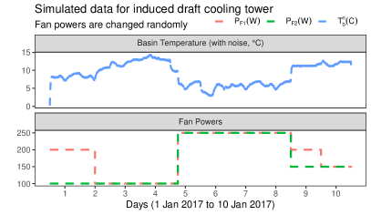
Fig. 6: Simulated data for the first 10 days of 2017.

$t_{n}$	$P_{F1}$	$P_{F2}$	$Q_{p}$	$T_{b}$	$T^{n}_{b}$
(time)	(W)	(W)	(W)	(K)	(K)
0.000694	100	100	33	10	10.020
0.001388	100	100	33	10	10.023
…	…	…	…	…	…

TABLE I: Simulated data ($T^{n}_{b}$ is noisy basin temperature).

V-B Training

Two black-box models (NN and LSTM) and three grey-box models (PhyNN, PhyLSTM${}_{\textit{WF}}$ and PhyLSTM${}_{\textit{WOF}}$) are trained and evaluated. The noisy temperature of basin ($T^{n}_{b}$) is used as an output to train these models, and the power of the fans ($P_{F1}$ and $P_{F1}$) and timeslot ($t_{n}$) are used as inputs. Time ($t_{n}$) is fed as a decimal value ($t_{n}$$~{}\in~{}$(0.00, 24.00), as described in Section V-A).

We use the simulated data for 2017 described in Section V-A to train the data-driven models. We define multiple training and validation sets using a walk forward moving window validation (Fig. 7). This validation is conducted because the basin temperature is time series data. All models are trained for training period $\in\{1,3,5,7\}$ months of training data (with 30 days in each month) with a moving window of 30 days, and a total of five validation sets are applied for each number of training months. We train models on different numbers of training months to evaluate the impact of training data on the model performance. To train the model, we select data in the training duration from the 2017 data, and use Algorithm 1 to optimize the weights of the model. Each trained model is evaluated for the next five days immediately following the end of the training period.

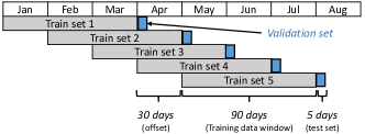
Fig. 7: Walk forward-moving window validation for training period of three months (90 days).

All models are defined using TensorFlow in Python. The weights of the models are optimized by minimizing the loss functions defined in Section IV-C using ADAM optimization for 1,000 iterations and a learning rate of 0.001. We use the Limited-memory BFGS optimization algorithm provided by the Python library Scipy with a maximum of 5,000 function evaluations to complete the training. The remaining parameters of the optimizers’ are set to their default values.

Black-box and grey-box models have fully connected networks. Each network has three input nodes, one output node, and two hidden layers with 16 neurons in each hidden layer. In the case of PhyLSTM${}_{\textit{WF}}$, one extra input node is added to feed the output of the previous timestep. For all LSTM-based models (black-box LSTM as well as grey-box PhyLSTM${}_{\textit{WOF}}$) and PhyLSTM${}_{\textit{WF}}$), the hidden layers have 16 LSTM cells each. Sigmoid activation is used for all networks. We choose sigmoid because, we observed that ReLU activation made the LSTM model diverge [23]. Model performances were compared for tanh and sigmoid activation functions with one, two and three hidden layers, where we note that sigmoid with two hidden layers provided faster and more accurate convergence.

Physics informed LSTM networks are optimized for the recurrence of k = 60 timesteps (60 min). The RNN is trained using the ‘teacher-forcing’ algorithm introduced in [24] where we use the previous timesteps’ ground truth to train the network, i.e., during training, the real value of the previous timestep is used as input as opposed to the value estimated from PhyLSTM. While making predictions from PhyLSTM, we feed the data for the last $k$ timesteps to make the prediction. The time derivative of the basin temperature is calculated using the auto differentiation functionality provided by the TensorFlow platform.

V-C Evaluation

We evaluate the performance of the data-driven models using absolute errors encountered in estimating the system response, i.e., the basin temperature. The absolute error for each timestep for a data-driven model $m$ is defined in Eq. (21), where $T_{b,i}$ is the basin temperature simulated using the white-box model, and $\widehat{T}^{m}_{b,i}$ is the estimated basin temperature (using data-driven model $m$ $\in\{\text{NN},~{}\text{LSTM},~{}\text{PhyNN},~{}\text{PhyLSTM}_{\textit{WOF}},~{}\text{PhyLSTM}_{\textit{WF}}\}$).

$$|e_{i}|^{m}=|T_{b,i}-\widehat{T}^{m}_{b,i}|$$ (21)

Absolute errors are calculated for all models trained on different training periods ($\in\{$1, 3, 5, 7$\}$ months) for each timestep in the immediate next 5 days, i.e., for the next 7,200 minutes (timesteps). We also compare the training time for all models, i.e., the time it takes to run each iteration of optimization. The performance of data-driven models is compared for three periods of prediction: (i) short-term, i.e., based on absolute errors of the immediate-next one hour (60 min) (ii) intermediate-term, i.e., based on absolute errors of the immediate-next one day (1,440 min) (iii) and long-term, i.e., based on absolute errors of the immediate-next five days (7,200 min) .

To analyze the accuracy of estimated flexibility metrics, we calculate the Mean Absolute Error (MAE) for the estimated $\widehat{SoC}$ (Eq. (19)). Additionally, we study the available and estimated operational flexibility for the given prediction horizon ($short$-$term$, $intermediate$-$term$, $long$-$term$). This is presented as a 2D region defined by $RoC$ on the x-axis and $SoC$ on the y-axis [17]. Available operational flexibility is defined by the operational limits of the cooling tower (Section V-A). We compare the proposed models’ evaluation time (i.e., time required to predict basin temperature for each timestep) and evolution of the training loss with the number of iterations.

VI Experimental Results

VI-A Performance of grey-box models (Q1–Q2)

To answer Q1 and Q2, we study the absolute errors encountered in the data-driven models for all three prediction horizon (short-term, intermediate-term, and long-term). Figure 8 compares the absolute errors in prediction for data-driven models optimized using data from training-period of seven months (210 days). Absolute errors for all 5 validation sets are used to construct each box.

For short-term, black-box NN and grey-box PhyNN have statistically similar absolute errors. Variance of grey-box PhyLSTM${}_{\textit{WOF}}$ (physics informed LSTM without feedback of basin temperature, Section IV-B2) is significantly lower compared to the black-box LSTM, indicating that enforcing physics improves the precision of the model. Among all models, we note the lowest absolute errors for PhyLSTM${}_{\textit{WF}}$, where the physics is enforced and feedback is applied. Since the performance of models of the short-term horizon impacts the control effectiveness based on these models, we can conclude that PhyLSTM${}_{\textit{WF}}$ has a high potential for control design, with less than 5% error across all validation sets.

Intermediate-term predictions (the next 24 h) can be used to make pricing decisions based on day-ahead prices, required power, etc. Both Physics based LSTM networks (PhyLSTM${}_{\textit{WF}}$ and PhyLSTM${}_{\textit{WOF}}$) outperform the black-box NN and LSTM for intermediate-term, however, compared to short-term the error increases. We also note the error reduction for PhyLSTM${}_{\textit{WOF}}$ compared to the black-box LSTM, indicating improvement in model performance by enforcing system dynamics into the network. Similar conclusions can be drawn from the data-driven models for long-term performance, where we note statistically similar performance for both physics informed LSTM networks.

While reduction in modeling error by integrating physics on neural networks has been noted in the past [11], our PhyNN and NN have similar errors in all prediction periods for the selected ECS configuration (2 fans).

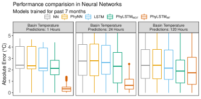
Fig. 8: Absolute error for short-term, intermediate-term, and long-term models trained for seven months (210 days). Each box contains data for all test sets. (For example, a box in the long-term has: 5 test sets$\times$60 minutes$\times$120 hours.)

VI-B Impact of training data (Q3)

To study the impact of the amount of training data on performance, optimization, and evaluation time of data-driven models (Q3), we study the absolute errors and training loss for all training periods ($\in\{1,3,5,7\}$). Fig. 9 shows the absolute errors for intermediate-term (24 hours) for all training periods. Solid colored lines represent the average absolute error across all validation sets, and the grey area is the 25 to 75 percentile.

VI-B1 Accuracy comparison

We compare the accuracy of models using absolute error encountered in estimation. Increasing the amount of training data improves the performance of the grey-box PhyLSTM${}_{\textit{WF}}$ model, i.e., we get the lowest absolute errors for PhyLSTM${}_{\textit{WF}}$ trained with seven months of training data. The performance of the PhyLSTM${}_{\textit{WF}}$ improves with the size of training data as seen in Fig. 9 (decrease in average and variance of error across all validation sets). This happens because the model learns the time-dependent behavior of the process accurately from the system dynamics and the network feedback. We notice a similar performance characteristics for short-term and long-term.

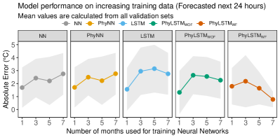
Fig. 9: Absolute errors for intermediate-term basin temperature predictions (24 hours) for all training periods. Each training month has 30 days of training data. Coloured line: Average absolute error; Shaded region: 25-75 percentile.

The absolute error for black-box NN and grey-box PhyNN is higher for models trained for 7 months of training data, in contrast to models trained for 1 month of training data. The data representing system dynamics of immediately preceding 1 month train a better model compared to the immediately preceding 7 months, because for 7 months the model has to generalize for multiple months (i.e., 7 months include various seasons, that have different outside temperature ranges). Their performance for training data for 3 and 5 months remains statistically similar. Additionally, we note no significant impact of training data on the variance of errors in both NN and PhyNN.

VI-B2 Training loss comparison

We study the evolution of training loss during training to see how different neural networks are optimized. In the case of a black-box NN, the loss consists of a mean square error MSE on the temperature of the basin (Eq. (16)). Training loss converges in approximately 500 iterations with 1 month of training data. Additionally, it takes fewer iterations for loss to converge for more training data, i.e., 3, 5, 7 months.

The loss for grey-box models (PhyNN and PhyLSTM${}_{\textit{WF}}$) comprises the mean squared error in $T_{b}$ and f (Eq. (17) and Eq. (18)). We notice that enforcing the dynamics of the process in the neural network models provides faster convergence, i.e., training loss converges in approximately 300 iterations for PhyNN and 150 iterations for PhyLSTM${}_{\textit{WF}}$, with 1 month of training data (compared to 500 iterations for NN). Furthermore, PhyLSTM${}_{\textit{WF}}$ also converges in fewer iterations with more training data. It takes approximately 100 iterations for the training loss to converge with a training data window of 7 months. We can conclude that PhyLSTM${}_{\textit{WF}}$ converges faster with more training data in contrast to PhyNN and NN.

VI-B3 Computation time comparison

We compare the computation time of data-driven models. Training time is higher in the case of PhyLSTM${}_{\textit{WF}}$ when compared to NN and PhyNN. One reason for this is the higher complexity of LSTM cells in PhyLSTM${}_{\textit{WF}}$ compared to the simple activation-based neurons in the other two models. This complexity results in more calculations while training the LSTM based models, increasing the overall training time. Each iteration for PhyLSTM${}_{\textit{WF}}$ takes approximately 0.15 s compared to 0.02 s in case of PhyNN and 0.001 s in case of NN. For our models, we notice that NN and PhyNN have the shortest evaluation time, with less than 5 ms on average to make each prediction. For PhyLSTM${}_{\textit{WF}}$ it takes 15 ms on average to make each prediction. For example, it takes 0.09 s (= 60 $\times$ 15 ms) for short-term (60 timeslots). We noted that for all proposed models the time to generate each prediction is small ($\ll$ 1 s) compared to the one-minute timeslot.

In summary, integrating physics provides faster convergence in data-driven grey-box models compared to the black-box NN. In grey-box models, PhyLSTM${}_{\textit{WF}}$ has a lower prediction error compared to all other models, and overall less than 5% error compared to the white-box model. With more training data, the accuracy of PhyLSTM${}_{\textit{WF}}$ increases, and it reaches convergence earlier.

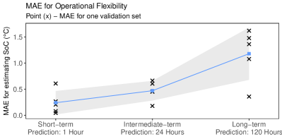
Fig. 10: MAE in State of Charge (${SoC}$) for PhyLSTM${}_{\textit{WF}}$.

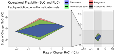
Fig. 11: Available and estimated operational flexibility for PhyLSTM${}_{\textit{WF}}$. (Operational limits are defined by upper and lower limits of $SoC$ and $RoC$)

VI-C Operational flexibility (Q4)

We calculate operational flexibility metrics ${SoC}$ and ${RoC}$ using the estimates from our data-driven PhyLSTM${}_{\textit{WF}}$ to answer (Q4). Figure 10 provides the Mean Absolute Errors (MAE) encountered in estimating $\widehat{SoC}$ for different prediction periods. These results are for the PhyLSTM${}_{\textit{WF}}$ trained with 7 months of training data. The MAE is lower in short-term predictions compared to intermediate-term and long-term predictions.

We present the estimated and available operational flexibility in Fig. 11, where the $x$-axis is ${RoC}$ and the $y$-axis is ${SoC}$. The grey area represents operational limits that define the available operational flexibility (Section V-A). White-box model and PhyLSTM${}_{\textit{WF}}$ provide similar regions for estimated operational flexibility. Additionally, we notice that the area of this region (representing estimated flexibility) increases with the period of prediction, i.e., larger flexibility in the long-term compared to the short-term. This behavior is due to the longer duration, which allows for a broader range of operational settings during data simulation.

VII Conclusions

Identifying system behavior in an energy-intensive Evaporative Cooling System (ECS) is critical for flexibility identification, building control policies, etc. In this paper, we define novel data-driven models for system identification in ECS. More specifically (i) we define grey-box physics informed networks (PhyNN, PhyLSTM${}_{\textit{WOF}}$ and PhyLSTM${}_{\textit{WF}}$) (ii) we choose an industrial process, i.e., an induced draft cooling tower, that offers operational flexibility to define a white-box model to simulate training data, and (iii) we evaluate the performance of our proposed grey-box models by training them for different training data sizes and validation sets. From our analyses, we conclude the following:

1. PhyLSTM${}_{\textit{WF}}$, i.e., a physics informed LSTM model with feedback (Section IV-B2) outperforms the grey-box (PhyNN and PhyLSTM${}_{\textit{WOF}}$) and black-box (NN and LSTM) models, where we see that it has less than 2% error for a short-term prediction horizon (Fig. 8). Similar performance is observed for an intermediate-term prediction horizon, and we can conclude that a physics informed LSTM has the highest accuracy among the data-driven models.

2. The performance of the PhyLSTM${}_{\textit{WF}}$ improves with longer training data window, as opposed to PhyNN and NN (as noted by the decrease in average and variance of absolute error in Fig. 9). Furthermore, PhyLSTM${}_{\textit{WF}}$ can be trained in fewer iterations with more data. It takes approximately 100 iterations for the training loss to converge for 7 months of training data.

3. The computation time to predict the future state of the process is insignificant ($\ll$ 1 s) compared to the time it takes to evaluate and implement control decisions in demand response (order of minutes). Such property makes the grey-box models suitable to be used to develop the control policies.

Overall the proposed physics informed LSTM network has excellent potential for developing flexibility identification that can be employed for estimating operational flexibility in an industrial energy intensive process such as an ECS (Fig. 11). In future research, we will (i) evaluate these grey-box models’ potential in developing effective control policies for industrial systems, (ii) explore these networks’ performance for multiple inputs and multiple outputs systems compared to the single output system that we tested, and (iii) quantitatively assess the effectiveness of PhyLSTM${}_{\textit{WF}}$ in other real-world applications .

Manu Lahariya is working towards a Ph.D. degree in computer science engineering (specializing in machine learning for energy applications) with the research group Artificial Intelligence for Energy (AI4E) at IDLab, Ghent University, Ghent, Belgium. He received M.Tech. degree and B.Tech. degree in aerospace engineering from the Indian Institute of Technology, Kharagpur, India in 2016 and 2017, respectively. He has contributed to multiple European research projects (e.g., BIGG, InduFlex) and was a visiting researcher at Robust Autonomy and Decisions Lab, University of Edinburgh, Edinburgh, Scotland. His research interests include physics-based machine learning, reinforcement learning, deep learning, and statistical modeling for designing efficient control and system identification across different applications (e.g., smart grids, residential space heating, soft robotics, etc.).

Farzaneh Karami received the MSc degree in Control Engineering from the Iran University of Science and Technology, Tehran, Iran, in 2010, and pursued her PhD degree in Computer Science (specializing in Optimization and Operations Research) at KU Leuven, Belgium. Since 2020, she has been a postdoctoral researcher with the Department of Electromechanical, Systems and Metal Engineering, Ghent University, Core lab EEDT-DC, Flanders Make, Belgium. Her research interests include using tools from mathematical optimization to create natural, understandable, and data-driven solutions that provide essential insights into improving operations.

Chris Develder is associate professor with the research group IDLab in the Dept. of Information Technology (INTEC) at Ghent University – imec, Ghent, Belgium. He received the MSc degree in computer science engineering and a PhD in electrical engineering from Ghent University (Ghent, Belgium), in Jul. 1999 and Dec. 2003 respectively (as a fellow of the Research Foundation, FWO). He has stayed as a research visitor at UC Davis, CA, USA (Jul.-Oct. 2007) and at Columbia University, NY, USA (Jan. 2013 – Jun. 2015). He was and is involved in various national and European research projects (e.g., FP7 Increase, FP7 C-DAX, H2020 CPN, H2020 Bright, H2020 BIGG, H2020 RENergetic, H2020 BD4NRG). Chris currently leads two research teams within IDLab, (i) UGent-T2K on converting text to knowledge (i.e., NLP, mostly information extraction using machine learning), and (ii) UGent-AI4E on artificial intelligence for energy applications (e.g., smart grid). He has co-authored over 200 refereed publications in international conferences and journals. He is Senior Member of IEEE, Senior Member of ACM, and Member of ACL.

Guillaume Crevecoeur (°1981) received his Master and PhD degree in Engineering Physics from Ghent University in 2004 and 2009, respectively. He received a Research Foundation Flanders postdoctoral fellowship in 2009 and was appointed Associate Professor at Ghent University in 2014. He is member of Flanders Make in which he leads the Ghent University activities on sensing, monitoring, control and decision-making. With his team, he conducts research at the intersection of system identification, control and machine learning for mechatronic and industrial robotic systems. His goal is to endow physical dynamic systems with improved functionalities and capabilities when interacting with uncertain environments, other systems and humans.

References

- Metzger and Polakow [2011] M. Metzger and G. Polakow, “A survey on applications of agent technology in industrial process control,” IEEE Transactions on Industrial Informatics, vol. 7, no. 4, pp. 570–581, 2011.
- Wang and Hodge [2017] Q. Wang and B. Hodge, “Enhancing power system operational flexibility with flexible ramping products: A review,” IEEE Transactions on Industrial Informatics, vol. 13, no. 4, pp. 1652–1664, 2017.
- Yassin et al. [2013] I. M. Yassin, M. N. Taib, and R. Adnan, “Recent advancements & methodologies in system identification: A review,” Scientific Research Journal, vol. 1, no. 1, pp. 14–33, 2013.
- Chiuso and Pillonetto [2019] A. Chiuso and G. Pillonetto, “System identification: A machine learning perspective,” Annual Review of Control, Robotics, and Autonomous Systems, vol. 2, no. 1, pp. 281–304, 2019.
- Bohlin [2006] T. P. Bohlin, Practical grey-box process identification: theory and applications. Springer Science & Business Media, 2006.
- Viljoen et al. [2018] J. Viljoen, C. Muller, and I. Craig, “Dynamic modelling of induced draft cooling towers with parallel heat exchangers, pumps and cooling water network,” Journal of Process Control, vol. 68, pp. 34–51, 2018.
- Díaz-Mateus and Castro-Gualdrón [2010] F.-A. Díaz-Mateus and J.-A. Castro-Gualdrón, “Mathematical model for refinery furnaces simulation,” CT&F Ciencia, Tecnología y Futuro, vol. 4, no. 1, pp. 89–99, 2010.
- Simani [2005] S. Simani, “Identification and fault diagnosis of a simulated model of an industrial gas turbine,” IEEE Transactions on Industrial Informatics, vol. 1, no. 3, pp. 202–216, 2005.
- Khayyam et al. [2015] H. Khayyam, M. Naebe, O. Zabihi, R. Zamani, S. Atkiss, and B. Fox, “Dynamic prediction models and optimization of polyacrylonitrile (pan) stabilization processes for production of carbon fiber,” IEEE Transactions on Industrial Informatics, vol. 11, no. 4, pp. 887–896, 2015.
- Wen et al. [2019] S. Wen, Y. Wang, Y. Tang, Y. Xu, P. Li, and T. Zhao, “Real-time identification of power fluctuations based on lstm recurrent neural network: A case study on singapore power system,” IEEE Transactions on Industrial Informatics, vol. 15, no. 9, pp. 5266–5275, 2019.
- Raissi et al. [2019] M. Raissi, P. Perdikaris, and G. E. Karniadakis, “Physics-informed neural networks: A deep learning framework for solving forward and inverse problems involving nonlinear partial differential equations,” Journal of Computational Physics, vol. 378, pp. 686–707, 2019.
- Lutter et al. [2019] M. Lutter, C. Ritter, and J. Peters, “Deep lagrangian networks: Using physics as model prior for deep learning,” arXiv preprint:1907.04490, 2019.
- Baetens et al. [2019] J. Baetens, G. Van Eetvelde, G. Lemmens, N. Kayedpour, J. D. De Kooning, and L. Vandevelde, “Thermal performance evaluation of an induced draft evaporative cooling system through adaptive neuro-fuzzy interference system (anfis) model and mathematical model,” Energies, vol. 12, no. 13, pp. 2544–2561, 2019.
- Aras Nejad et al. [2017] M. Aras Nejad, H. Golmohamadi, A. Bashian, H. Mahmoodi, and M. Hammami, “Application of demand response programs to heavy industries: a case study on a regional electric company,” International Journal of Smart Electrical Engineering, vol. 6, no. 03, pp. 93–99, 2017.
- Barth et al. [2018] L. Barth, N. Ludwig, E. Mengelkamp, and P. Staudt, “A comprehensive modelling framework for demand side flexibility in smart grids,” Computer Science-Research and Development, vol. 33, no. 1, pp. 13–23, 2018.
- Stull [2011] R. Stull, “Wet-bulb temperature from relative humidity and air temperature,” Journal of Applied Meteorology and Climatology, vol. 50, no. 11, pp. 2267–2269, 2011.
- Ulbig and Andersson [2015] A. Ulbig and G. Andersson, “Analyzing operational flexibility of electric power systems,” International Journal of Electrical Power & Energy Systems, vol. 72, pp. 155–164, 2015.
- Heussen et al. [2010] K. Heussen, S. Koch, A. Ulbig, and G. Andersson, “Energy storage in power system operation: The power nodes modeling framework,” in 2010 IEEE PES Innovative Smart Grid Technologies Conference Europe (ISGT Europe), 2010, pp. 1–8.
- Hochreiter and Schmidhuber [1997] S. Hochreiter and J. Schmidhuber, “Long short-term memory,” Neural computation, vol. 9, pp. 1735–80, 12 1997.
- Siegelmann et al. [1997] H. Siegelmann, B. Horne, and C. Giles, “Computational capabilities of recurrent NARX neural networks,” IEEE Transactions on Systems, Man, and Cybernetics, Part B (Cybernetics), vol. 27, no. 2, pp. 208–215, 1997.
- Menezes Jr and Barreto [2008] J. M. P. Menezes Jr and G. A. Barreto, “Long-term time series prediction with the narx network: An empirical evaluation,” Neurocomputing, vol. 71, no. 16-18, pp. 3335–3343, 2008.
- wea [2020] (2020) Weather in belgium. [Online]. Available: https://www.timeanddate.com/weather/belgium
- Le et al. [2015] Q. V. Le, N. Jaitly, and G. E. Hinton, “A simple way to initialize recurrent networks of rectified linear units,” arXiv preprint:1504.00941, 2015.
- Williams and Zipser [1989] R. J. Williams and D. Zipser, “A learning algorithm for continually running fully recurrent neural networks,” Neural Computation, vol. 1, no. 2, pp. 270–280, 1989.