Analysis of relay-based feedback compensation of Coulomb friction

Abstract

Standard problem of one-degree-of-freedom mechanical systems with Coulomb friction is revised for a relay-based feedback stabilization. It is recalled that such a system with Coulomb friction is asymptotically stabilizable via a relay-based output feedback, as formerly shown in [1]. Assuming an upper bounded Coulomb friction disturbance, a time-optimal gain of the relay-based feedback control is found by minimizing the derivative of the Lyapunov function proposed in [2] for the twisting algorithm. Furthermore, changing from the discontinuous Coulomb friction to a more physical discontinuity-free one, which implies a transient presliding phase at motion reversals, we analyze the residual steady-state oscillations. This is in the sense of stable limit cycles, in addition to chattering caused by the actuator dynamics. The numerical examples and an experimental case study accompany the provided analysis.

I INTRODUCTION

The dry Coulomb friction in mechanical systems, whose resistive force assumes either of two extreme values differing in the sign opposite to the direction of relative motion, has always been a ’classical’ but, at the same time, challenging example of switching dynamics. This may also require a switching control, see e.g. in [3]. The challenges in compensating for the Coulomb friction are rooted in two facts. One is that it presents a non-vanishing perturbation at zero equilibrium; and another (even more challenging) one is that it is subject to eventual discontinuities at the velocity zero crossing. Among the model-free compensation methods aimed for attenuating the effect of Coulomb friction on the controlled motion, the relay-based and also sliding-mode-based strategies (see e.g. [4] for basics) seem to be promising due to their robustness. Worth mentioning that the characteristics of frictional systems are mostly uncertain and/or perturbed, like for example the Coulomb friction coefficient can be both time- and state-varying, depending on such factors as the ambient temperature, surface dust, normal load, dwell time, wear, lubrication and others.

In this work, we recall and extend the analysis of the relay-based feedback compensation of the Coulomb friction provided in [1], however based on the same principles as the widely celebrated sliding-mode twisting algorithm [5]. Our goal is to analyze the convergence behavior of the stabilizing relay-based compensator of the Coulomb friction and to derive the time-optimal parametric conditions for its tuning. We are also addressing the possible occurrence of the steady-state harmonic oscillations and distinguish their causes by analyzing more physical discontinuity-free friction transitions in the so-called presliding region of a motion initiation or motion reversal. Therefore, both the rather classical discontinuous Coulomb friction law and its tribology-justified, discontinuity-free extension to a smooth force-displacement mapping during presliding will be treated.

The rest of the paper is organized as follows. In section II, we describe the considered class of mechanical systems with Coulomb friction, thus formulating the problem statement. In section III, we analyze the relay-based feedback control regarding its time-optimal parametrization, while using analysis of the continuous Lyapunov function provided in [2] for the twisting algorithm. In section IV, we elaborate on the residual steady-state oscillations, while introducing the discontinuity-free Coulomb friction behavior and discussing the appearance of the associated stable limit cycles. Also the possible appearance of an inherent and, moreover, overlapped chattering, in case of additional actuator dynamics, is recalled in accord with [6, 7]. In section V, we present an illustrative experimental case study of compensating the Coulomb friction. The theoretical and experimental results of the paper are summarized and discussed in section VI.

II MECHANICAL SYSTEM WITH COULOMB FRICTION

We consider a feedback controlled one-degree-of-freedom mechanical system with discontinuous Coulomb friction, i.e. $-C_{f}\,\mathrm{sign}(x_{2})$, which closed-loop dynamics is described by

$$\left(\begin{array}[]{c}\dot{x}_{1}\\ \dot{x}_{2}\\ \end{array}\right)=\underset{\equiv g}{\underbrace{\left(\begin{array}[]{cc}0&1\\ -k&-c-C_{f}/|x_{2}|\\ \end{array}\right)\left(\begin{array}[]{c}x_{1}\\ x_{2}\\ \end{array}\right)}}+\left(\begin{array}[]{c}0\\ 1\\ \end{array}\right)u.$$ (1)

A state-feedback control, which is equivalent to a standard PD (proportional-derivative) position controller, is parameterized within the system matrix coefficients $k,c>0$. A unity inertia of the system is assumed for the sake of simplicity and without loss of generality. The maximal (i.e. upper bounded) Coulomb friction coefficient $C_{f}>0$ is assumed to be known, and both dynamic states of a relative motion $(x_{1},x_{2})(t)$ are assumed to be available. Note that the input control channel $u$ is used for the sake of friction compensation we are mainly interested in here. Next, we will first show that an unforced system (1) will always approach the $x_{1}$-axis for all $t>t_{0}$, independently of the initial conditions $t_{0}\geq 0$, $\|x_{1}(t_{0}),x_{2}(t_{0})\|<\infty$. When doing this, we will closely follow the developments provided in [1].

Assuming a positive definite and radially unbounded Lyapunov function candidate $V_{g}(x_{1},x_{2})=0.5\,kx_{1}^{2}+0.5\,x_{2}^{2}$, and taking its time derivative, one obtains

$$\dot{V}_{g}=-cx_{2}^{2}-C_{f}|x_{2}|<0\quad\forall\;x_{2}\neq 0.$$ (2)

Since $\dot{V}_{g}$ is negative definite everywhere except $x_{1}$-axis, the unforced trajectories of the system (1) prove to reach always the manifold $\Lambda=\{(x_{1},x_{2})\in\mathbb{R}^{2}:x_{2}=0\}$ as $t\rightarrow\infty$. Note that this is independent of the assigned control parameters $k>0$ and $c\geq 0$. Here $c>0$ is in the sense of an exponentially stable linear feedback system if $C_{f}=0$; and $c=0$ implies a finite-time stability for the nonlinear damping $C_{f}>0$. Next, let us analyze the behavior of state trajectories when approaching the $\Lambda$-manifold from two disjoint regions

$$P^{+}=\{x\in\mathbb{R}^{2}:x_{2}>0\}\;\hbox{ and }\;P^{-}=\{x\in\mathbb{R}^{2}:x_{2}<0\}$$

of the $(x_{1},x_{2})\equiv x\in\mathbb{R}^{2}$ phase-plane. Since the signum operator, which determines the Coulomb friction dynamics, is defined in zero as $\mathrm{sign}(0)\in[-1,+1]$ (i.e. in the Filippov sense [8]) the vector field $g$ on the discontinuity manifold is

$$g^{+}(x_{\Lambda}) ={\underset{x\rightarrow x_{\Lambda},\>x\in P^{+}}{\lim}}g(x)=\left(\begin{array}[]{c}0\\ -kx_{1}-C_{f}\end{array}\right),$$ (5)

$$g^{-}(x_{\Lambda}) ={\underset{x\rightarrow x_{\Lambda},\>x\in P^{-}}{\lim}}g(x)=\left(\begin{array}[]{c}0\\ -kx_{1}+C_{f}\end{array}\right).$$ (8)

From (5), (8) it is visible that the velocity vectors are pointing in opposite directions for $|x_{1}|\leq C_{f}k^{-1}$. Since both vector fields are normal to the manifold $\Lambda$, neither continuous motion nor sliding mode will occur within

$$\Lambda_{I}=\{(x_{1},x_{2})\in\mathbb{R}^{2}:\>-C_{f}k^{-1}\leq x_{1}\leq C_{f}k^{-1},\,x_{2}=0\}.$$

This forms the largest invariant set $\Lambda_{I}$ on the $x_{1}$-axis which coincides with the range of residual control errors for the class of motion systems (1) perturbed by the Coulomb friction with discontinuity. On the contrary, both vector fields (5), (8) are pointing in the same direction, towards $P^{+}$ for $x_{1}<-C_{f}k^{-1}$ and towards $P^{-}$ for $x_{1}>C_{f}k^{-1}$, in which way a continuous motion resumes to take place.

The above results, cf. with [1], are well known in the control engineering practice, when an output feedback controller is confronted with the issues of non-compensated nonlinear friction. Note that adding an integral control part to (1) will not resolve convergence to stable zero equilibrium, as has been recently demonstrated and discussed in [9].

III RELAY-BASED FEEDBACK

A stabilizing relay-based feedback control

$$u=-\gamma\,\mathrm{sign}(x_{1})$$ (9)

was analyzed in [1] for the second-order systems with discontinuous Coulomb friction, cf. section II. Note that in absence of the linear sub-dynamics in (1), i.e. if $k,c=0$, the control system (1), (9) will coincide with the well-known twisting algorithm [5], except that the velocity feedback part $-C_{f}\,\mathrm{sign}(x_{2})$ is no longer a control design term, but the given inherent feature of the plant, namely the Coulomb friction, cf. (1). It is well known that for an unperturbed double integrator system, the twisting algorithm requires $\gamma>C_{f}$ for ensuring a finite-time exact convergence of $(x_{1},x_{2})(t)$-trajectories to the stable zero equilibrium. When the double integrator with relays feedback is augmented by the residual system dynamics, i.e. $k,c\neq 0$, one still needs analyzing the $\gamma/C_{f}>1$ ratio for optimizing the convergence time of the feedback compensator (9), provided the stable gains $k$ and $c$ are given. Below, we will follow and use, while adapting for (1), (9), the Lyapunov function analysis of the twisting algorithm developed and presented in [2].

Introducing the upper and lower bounds $U>U^{*}>0$ of the matched control and perturbation quantities of (1), (9) as

$$U=\gamma+C_{f}-F,\quad U^{*}=\gamma-C_{f}+F$$

cf. [2, section III], the continuous Lyapunov function [2]

$$V(x)=\left\{\begin{array}[]{ll}\alpha_{1}|x_{2}|+\alpha_{2}\sqrt{x_{2}^{2}+2U|x_{1}|},&x_{1}x_{2}>0\\[2.84526pt] \alpha_{3}|x_{2}|+\alpha_{4}\sqrt{x_{2}^{2}+2U^{*}|x_{1}|},&x_{1}x_{2}\leq 0.\\ \end{array}\right.$$ (10)

can be used. Here, the collected coefficients are

$$\alpha_{1}=\frac{1}{U},\>\alpha_{2}=\frac{r^{-1}+r}{U(1-r)},\>\alpha_{3}=-\frac{1}{U^{*}},\>\alpha_{4}=\alpha_{1}+\alpha_{2}-\alpha_{3}$$

with $r=\sqrt{U^{-1}U^{*}}$. Beyond that, it was proved [2, Theorem 3.1] that the Lyapunov function’s time derivative is

$$\dot{V}\leq\left\{\begin{array}[]{ll}-1,&x_{1}x_{2}>0,\\[2.84526pt] -\frac{\gamma-C_{f}-F}{\gamma+C_{f}+F},&x_{1}x_{2}<0,\\ \end{array}\right.$$ (11)

and the convergence time $T^{*}$ satisfies

$$T^{*}\leq\left\{\begin{array}[]{ll}V\bigl{(}x(0)\bigr{)},&x_{1}(0)x_{2}(0)>0,\\[2.84526pt] r^{2}V\bigl{(}x(0)\bigr{)},&x_{1}(0)x_{2}(0)<0.\\ \end{array}\right.$$ (12)

It can be seen from (11) that for the closed-loop system to be asymptotically stable, the relay control gain must satisfy $\gamma>C_{f}+F$. Furthermore, one can recognize from (12) that the convergence in the I-st and III-rd quadrants of the phase-plane is not faster than in the II-nd and IV-th quadrants, due to $r<1$. We will make good use of this fact when next analyzing the time-optimal feedback gain of a relay-based Coulomb friction compensation. Further it is essential to notice that the linear sub-dynamics in (1) appears instead of the $F$-bounded perturbation term of a double integrator with feedback of both relays. Therefore, and without lose of generality for (1), (9), we will set $F=0$ and solely requires that the roots of the characteristic equation $\lambda^{2}+c\lambda+k=0$ are all negative, where $\lambda$ is the complex Laplace variable.

Since the convergence time estimates (12) differ by the multiplicative factor $r^{2}$, it is reasonable to look into the convergence of those trajectories which start, correspondingly, initially proceed in either II-nd or IV-th quadrant. Note that from an application-related perspective it is fully in line with the situation where an $x_{1}$-set-point is the control objective, while $x_{2}(0)=0$ means there is no relative motion at the initial time $t=0$. Evaluating the second case of (10), with $F=0,\>x_{2}(0)=0$, and multiplying with $r^{2}$, cf. (12), one obtains the upper bound of the time estimate as

$$T\equiv\frac{\gamma\Bigl{(}1+\sqrt{\frac{\gamma-C_{f}}{\gamma+C_{f}}}\Bigr{)}}{\gamma C_{f}+C_{f}^{2}}\,\sqrt{2(\gamma-C_{f})|x_{1}|}.$$ (13)

Taking the derivative of (13) with respect to $\gamma$ and evaluating numerically $\partial T/\partial\gamma=0$, one can find minima of the upper bound $T$ and, thus, the time-optimal ratio $\gamma/C_{f}=1.119$.

The convergence time upper bound versus the control parameter ratio $\gamma/C_{f}$ is shown exemplary in Fig. 1, for the different $x_{1}(0)$ initial values in (a) and Coulomb friction coefficients $C_{f}$ in (b). Here $T_{0}$ denotes a boundary case where the control gain $\gamma^{+}\rightarrow C_{f}$ approaches Coulomb friction coefficient from the right. One can recognize that for selecting the time-optimal $\gamma$-gain, a possible variation of the Coulomb friction parameter about the range of 40% will not worsen the convergence performance comparing to $T_{0}$.

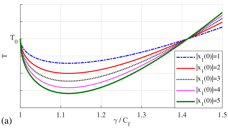
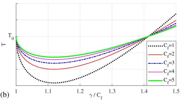
Figure 1: The convergence time (unitless) upper bound versus the $\gamma/C_{f}$ ratio: for the various initial conditions in (a), and various $C_{f}$ values in (b).

IV CONVERGENCE WITH LIMIT CYCLES

Next, we are addressing the problem of residual steady-state oscillations which appear in form of the stable limit cycles. It is worth noting that these should not be confused immediately with the well-known chattering effect in sliding-mode applications, see e.g. [10, 11, 12]. The latter can well occur upon the convergence of the control system (e.g. in twisting mode) to zero equilibrium for a relative degree of the overall plant (i.e. process and actuator) higher than two, see [6]. For ensuring that this is not a case for the system (1), (9) we will first briefly recall the concluding statements of analysis provided in [6] for the second-order twisting algorithm. Then, we will introduce the discontinuity-free transients of Coulomb friction, known as presliding friction, and address the occurrence of the stable limit cycles owing to smooth transitions of the friction force.

IV-A Assessment of chattering by harmonic balance

The describing function (DF) analysis, developed for the twisting algorithm in [6], can be applied directly to the system (1) with discontinuous Coulomb friction and relay-based feedback control (9). A parallel feedback of two relay operators, one with the gain factor $\gamma$ and one with the Coulomb friction coefficient $C_{f}$, allows writing the DF, denoted by $\Omega(\cdot)$, as a sum of both DFs, i.e.

$$\Omega=\Omega_{\gamma}+j\omega\,\Omega_{C_{f}}=\frac{4\gamma}{\pi A_{1}}+j\omega\frac{4C_{f}}{\pi A_{2}}=\frac{4}{\pi A_{1}}(\gamma+jC_{f}),$$ (14)

where $\omega$ and $A_{1}$ are the angular frequency and amplitude of the first harmonic of periodic oscillations of $x_{1}(t)$ at steady-state, cf. [6]. For convenience of the reader, we recall that: (i) $A_{2}=A_{1}\omega$, due to the relationship between $x_{1}$ and $x_{2}=dx_{1}/dt$ in Laplace domain, and (ii) the DF of an $\sigma$-amplified relay is $\Omega(A)=4\sigma\,(\pi A)^{-1}$. For proving the existence, correspondingly finding the parameters, of the harmonic oscillations (i.e. chattering), the corresponding harmonic balance equation

$$-\frac{1}{\Omega(A_{1})}=G(j\omega)\equiv\frac{1}{-\omega^{2}+j\omega c+k}$$ (15)

has to be solved. $G(j\omega)=x_{1}(j\omega)/u(j\omega)$ is the input-to-output transfer function of the linear part of the system (1), i.e. when excluding the Coulomb friction term out from the states equation (1). Note that the graphic of $-1/\Omega(A_{1})$ is a straight line, which is starting from the origin and progressing in negative direction (within II-nd quadrant of the complex plane) as the amplitude $A_{1}$ increases. The angle, correspondingly the slope, of that line is equal to $\arctan(C_{f}/\gamma)$, cf. [6]. Obviously, for any physical (i.e. positive) parameter values of $k,\,c,\,\gamma,\,C_{f}$, there is no intersection point of the Nyquist plot of $G(j\omega)$ with $-1/\Omega(A_{1})$ plot of the DF. That means no $(\omega,A_{1})$-solution of (15) exists which implies no harmonic oscillations can appear upon the convergence in twisting mode of the control system (1), (9).

IV-B Discontinuity-free Coulomb friction

The discontinuity-free transients of the Coulomb friction at each motion reversal (at time instant $t=t_{r}$) can be captured in different manner, while fulfilling the rate-independency and providing the so-called presliding hysteresis loops, cf. e.g. [13]. Yet, according to the tribological study [14], the area of presliding hysteresis loops increases proportionally to the 2nd power of the so-called presliding distance $z(t)$, which captures the magnitude of relative displacement after the sign of the relative velocity changes, see [13] for details. Using the scaling factor $s>0$, which relates an after-reversal motion to the presliding distance as

$$z=s\int\limits^{t}_{t_{r}}x_{2}\,dt,$$ (16)

defined on the interval $z\in[-1,\,0)\cup(0,\,1]$, one can describe the branching of frictional force during presliding by

$$f_{0}(z)=z\bigl{(}1-\ln(z)\bigr{)}.$$ (17)

Each motion reversal at $t_{r}$ gives rise to a new presliding transition captured by (16), (17), so that the total (normalized) presliding friction map, cf. [13], is

$$f_{p}(t)=\bigl{|}\mathrm{sign}(x_{2})-f_{r}\bigr{|}\,z\bigl{(}1-\ln(z)\bigr{)}+f_{r}.$$ (18)

The memory state of the last reversal transition is $f_{r}:=f_{p}(t_{r})$, cf. exemplified curves in Fig. 2. Since the presliding friction mapping (18) is defined for $|z|\leq 1$ only, the overall continuous Coulomb friction force is given by

$$f(t)=\left\{\begin{array}[]{ll}C_{f}\,f_{p}(t),&\hbox{if }|z|\leq 1,\\[2.84526pt] C_{f}\,\mathrm{sign}\bigl{(}x_{2}(t)\bigr{)},&\hbox{otherwise.}\\ \end{array}\right.$$ (19)

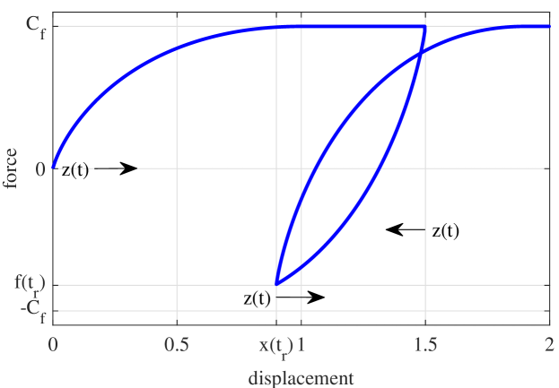
Figure 2: Continuous transients of Coulomb friction at motion reversals.

IV-C Limit cycles in presliding range

We now want to prove the occurrence of stable limit cycles around zero equilibrium as a result of smooth frictional transitions upon the motion reversals described above. For the sake of simplicity and without loss of generality, we will in the following assume $k,\,c=0$, so that the linear sub-dynamics is excluded as less relevant for the main mechanisms of trajectory convergence and emergence of the limit cycles. Following to that, the closed-loop control system (1), (9) is reduced to the second-order dynamics

$$\ddot{x}_{1}+f(\dot{x}_{1})+\gamma\,\mathrm{sign}(x_{1})=0.$$ (20)

Assuming the Lyapunov function candidate $V_{f}=0.5\,\dot{x}_{1}^{2}+\gamma\,|x_{1}|$, which is positive definite everywhere and radially unbounded, one can easily obtain its time derivative as

$$\dot{V}_{f}=-\dot{x}_{1}\,f(\dot{x}_{1}).$$ (21)

First, considering the discontinuous Coulomb friction, one can directly show that

$$\dot{V}_{f}^{d}=-C_{f}\,|\dot{x}_{1}|<0\quad\forall\quad\dot{x}_{1}\neq 0.$$ (22)

This proves the system (20) will always reach $x_{1}$-axis and is, thus, globally stable within invariant set $\Lambda$, cf. section II. In order to demonstrate the system (20) is but globally asymptotically stable, we apply the LaSalle invariance principle and show that the invariant set contains only one point, namely $\Lambda_{e}\equiv(0,0)$. All trajectories starting from $\mathbb{R}^{2}\setminus\Lambda_{e}$ will reach $\Lambda$, at some time $t_{1}>0$, and then stay there for all $t>t_{1}$, according to (22).

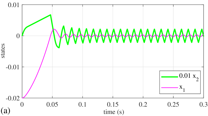
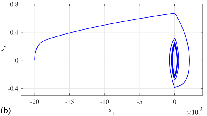
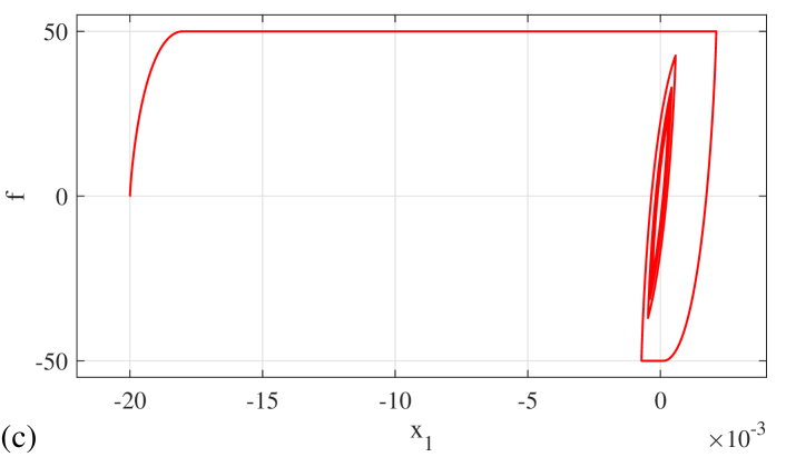
Figure 3: Numerical example: position and velocity (down-scaled by 0.01) in (a), states trajectory in (b), and friction-displacement curve in (c).

This implies $\ddot{x}_{1}=0\;\Rightarrow\;C_{f}\,\mathrm{sign}(\dot{x}_{1})=-\gamma\,\mathrm{sign}(x_{1})$. It is evident that for all positive parameter values this equality is impossible in the I-st and III-rd quadrant of the state-space, due to the same signs. Thus, the above equality can hold only in the II-nd and IV-th quadrant and iff $\gamma=C_{f}$. However, for any $\gamma>C_{f}$, cf. section III, the trajectory will immediately move out of the set $\Lambda$, which is a contradiction to its definition. Only in $\Lambda_{e}$, the $\ddot{x}_{1}=0$ is fulfilled that proves the global asymptotic convergence of the system (20) with $\gamma>C_{f}$ and $f(\dot{x}_{1})\equiv C_{f}\,\mathrm{sign}(\dot{x}_{1})$. Note that the Lyapunov function $V_{f}$ is weak, since not differentiable in $x_{1}=0$. Thus, an extended invariance principle (see e.g. [3]) must be applied for showing the asymptotic stability. Indeed, one can show that the gradient $\partial V_{f}/\partial x$ does not exist on the $x_{1}=0$ switching axis, which implies $x_{1}=\dot{x}_{1}=0$ is the unique solution, and there are neither blocking nor unstable sliding modes on the manifold $\bigl{\{}x\in\mathbb{R}^{2}\,|\,x_{1}=0\bigr{\}}\setminus\mathbf{0}$.

Next, assuming the continuous Coulomb friction (19), one can show that in the presliding vicinity to zero equilibrium, the time derivative is

$$\dot{V}_{f}^{c}=-C_{f}\dot{x}_{1}f_{p}(z).$$ (23)

Depending on the motion direction and the instantaneous sign of the presliding transition curve $f_{p}(z)$, the time derivative of the Lyapunov function candidate can be either positive or negative, cf. (23) and Fig. 2. For $\dot{V}_{f}^{c}(t)>0$ the system will increase the energy level and, in worst case, leave the presliding, meaning pass over to $f(\dot{x}_{1})=C_{f}\,\mathrm{sign}(\dot{x}_{1})$. At the same time, since the force-displacement transition curves $f_{p}(z)$ are always clockwise, they behave as dissipative on each closed cycle. That means the total $V_{f}^{c}(t_{2})-V_{f}^{c}(t_{1})=\Delta V_{f}^{c}<0$ for all $t_{2}>t_{1}$ which are the two consecutive time instants of a closed presliding cycle with $f_{p}(t_{2})=f_{p}(t_{1})$, cf. Fig. 2. Recall that the energy losses at such cycles are equivalent to the corresponding area of the force-displacement hysteresis loops. A stable limit cycle will occur once the input energy (i.e by the control $u=-\gamma\,\mathrm{sign}(x_{1})$) supplied between two reversal time instants $t_{2}$ and $t_{1}$ becomes equal to $\Delta V_{f}^{c}$. The size of the limit cycle is $<s^{-1}$ and depends on the $s$, $C_{f}$, and $\gamma$ parameters. An exact analysis of the size and period of the limit cycles go beyond the scope of the recent work and might be addressed in the future research. An illustrative numerical example, with $C_{f}=50$, $s=500$, $\gamma=60$, and $k,c=0$, is shown in Fig. 3. Both system states are depicted as time series in (a) and as a phase-plane trajectory in (b), while the friction force over the relative displacement in (c), respectively. One can recognize the appearance of a stable limit cycle, in accord with the above discussion.

V EXPERIMENTAL CASE STUDY

The relay-based feedback compensation of the Coulomb friction was experimentally evaluated in the following case study, accomplished on an electro-mechanical drive system in the laboratory setting, cf. Fig. 4.

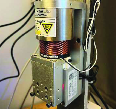
Figure 4: Experimental setup of electro-mechanical drive (laboratory view).

The electro-magnetically actuated voice-coil motor drive has the total linear stroke about 20 mm, which is indirectly measured by the contactless inductive displacement sensor with a nominal repeatability of $\pm 12$ $\mu m$. Note that due to a position-varying amplification gain of the voice-coil motor and the hardware-specific limitations of detection area of the contactless sensor, a narrow displacement range of 6 mm only was used in the following control experiments. The real-time board operates the system with the set sampling rate of 10 kHz, while the available control signal is the power-amplified voltage $V$ in the range $[0,\,10]$ V. Further details of the setup can also be found in [15], with a main difference that the additional oscillating payload is purposefully detached here from the drive.

The constant gravitational term $mg$, where $m=0.735$ kg is the overall moving mass and $g=9.8\,\mathrm{m}/\mathrm{sec}^{2}$ is the constant of acceleration of gravity, is pre-compensated so that the input-output system plant can be well described by the second-order dynamics (1). Note that the nominal electric time constant of 1.2 ms will be neglected.

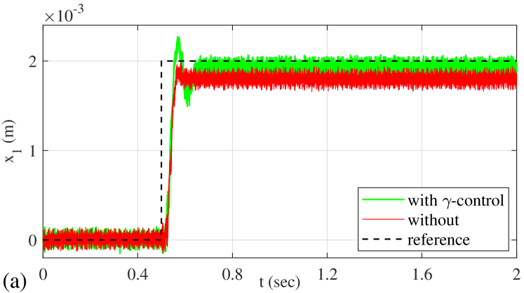
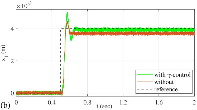
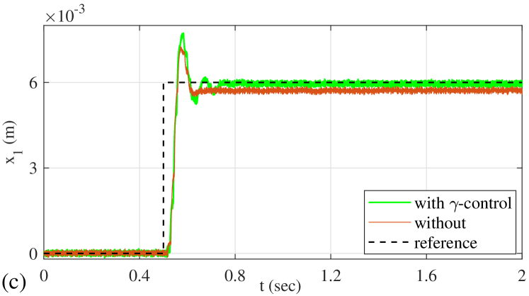
Figure 5: Experimentally evaluated step response of the control system with and without relay feedback compensator (9), with 2 mm reference step in (a), 4 mm reference step in (b), 6 mm reference step in (c).

Therefore, we assume there is no additional actuator dynamics to be taken explicitly into account, cf. with [6]. The system input signal is $u=\tau m^{-1}V$, where the motor force constant $\tau=3.28$ is determined as the ratio between the electromotive force constant and overall resistance of the coil and connections. The identified Coulomb friction coefficient is $C_{f}=1.148$ N and the set linear feedback parameters are $k=5600$ and $c=150$. The corresponding poles of the linear sub-dynamics in (1) are $\lambda_{1}=-70$ and $\lambda_{1}=-80$. It is worth noting that while the assigned $k$ is owned entirely by the linear output feedback gain (respectively scaled with $\tau m^{-1}$), the assigned $c$ value (equally scaled by $\tau m^{-1}$) includes both, the identified viscous system damping and the used output derivative feedback gain. The set relay gain is $\gamma=1.214$.

The experimentally evaluated step responses of the control system with and without relay feedback compensator (9) are shown in Fig. 5, for the step reference of 2 mm in (a), 4 mm in (b), and 6 mm in (c). The $\gamma$-compensated stiction in vicinity to the set reference, which is due to the Coulomb friction, cf. section II, is visible in all three experiments. For the time $t<0.5$ sec, where no control action appears, i.e. $V=0$, one can recognize a relatively high level of the measurement noise. Note that a theoretically expected residual position error range (when not compensating for friction cf. section II) is about $\pm 0.2$ mm, according to the $C_{f}/k$ ratio. The actually evaluated mean steady-state errors, for $t>0.8$ sec of all $\{2,\,4,\,6\}$ mm references, are $\{0.2,\,0.29,\,0.28\}$ mm without $\gamma$-compensator, and $\{0.07,\,0.06,\,0.04\}$ mm with $\gamma$-compensator, respectively. The residual control errors without $\gamma$-compensator appear in line with the theoretical analysis, while the residual control errors with $\gamma$-compensator are close to the measurement noise and, moreover, due to additional adhesion by-effects which are captured neither by discontinuous nor discontinuity-free Coulomb friction laws.

VI SUMMARY AND DISCUSSION

The relay-based feedback compensation of the Coulomb friction in second-order systems with one mechanical degree of freedom was analyzed. Since the closed-loop system with one output relay, due to the compensator, and another output-rate relay, due to discontinuous Coulomb friction law, is similar to the well-known twisting-algorithm [5], the existing approach of the corresponding continuous Lyapunov function [2] was used for the convergence analysis and determining a time-optimal relay gain. Further, it was described why a more physical discontinuity-free Coulomb friction, with the so-called presliding transients, will unavoidably lead to the stable limit cycles in vicinity to zero equilibrium. The uncompensated and feedback-relay compensated regulation of the output displacement were demonstrated in the experiments, where the residual steady-state error (due to stiction) is in accord with the theoretically expected one. Based on the results, reflections from analysis, and interpretation of the numerical simulations and control experiments, following points can be summarized for discussion.

• While the relative motion with discontinuous Coulomb friction is theoretically stabilizable by the output relay feedback, provided $\gamma>C_{f}$, a more physical actuator dynamics and, as a consequence, increase of the plant’s relative degree to become $>2$ will lead to harmonic oscillations of the output around equilibrium. This fact, which is in line with the DF-based analysis provided in [6], we observed experimentally when further increasing the $\gamma$-gain, even though it was admitted theoretically, cf. Fig. 1. An increase of the $\gamma$-gain will reduce the inclination angle of the $-1/\Omega(A_{1})$ slope, cf. section IV-A, and thus decrease the frequency and increase the amplitude of harmonic oscillations, as soon as the Nyquist plot of the overall plant with actuator will proceed also in the II-nd quadrant of the complex plane. Quantitatively it is directly visible since the amplitude of DF-determined harmonic oscillations is

  $$A_{1}=\frac{4}{\pi}\bigl{|}G(j\bar{\omega})\bigr{|}\sqrt{\gamma^{2}+C_{f}^{2}},$$ (24)

  cf. [7], where $\bar{\omega}$ is the solution (if it exists) of the harmonic balance equation (15). Therefore, not only the knowledge of (otherwise generally uncertain) $C_{f}$ is relevant for an optimal tuning of the $\gamma$ control gain, but also the acceptance level of the residual output oscillations, taking into account the actuator dynamics.

• Analysis of the discontinuity-free Coulomb friction behavior requires an accurate sensing of the relative displacement, with a possibly low level of both the measurement and process noise. On this account, the appearance of limit cycles due to presliding transitions could not be directly detected in the given experimental case study, despite such smooth force-displacement transitions are well known from the more accurate tribological investigations. An interesting point, which still requires both, more accurate position sensing and process knowledge, would be a decomposition of the residual output oscillations. Recall that it can include the components driven rather by additional actuator dynamics (i.e. due to relative degree $>2$) and those due to discontinuity-free Coulomb friction.

References

- [1] J. Alvarez, I. Orlov, and L. Acho, “An invariance principle for discontinuous dynamic systems with application to a Coulomb friction oscillator,” Journal of Dynamic Systems, Measurement, and Control, vol. 122, no. 4, pp. 687–690, 2000.
- [2] T. Sánchez and J. A. Moreno, “Lyapunov functions for twisting and terminal controllers,” in 13th International Workshop on Variable Structure Systems (VSS), 2014, pp. 1–6.
- [3] V. Utkin, Sliding modes in control and optimization. Springer, 1992.
- [4] Y. Shtessel, C. Edwards, L. Fridman, and A. Levant, Sliding mode control and observation. Springer, 2014.
- [5] S. V. Emel’yanov, S. K. Korovin, and L. Levantovskii, “Higher-order sliding regimes in binary control systems,” in Doklady Akademii Nauk, vol. 287, no. 6, 1986, pp. 1338–1342.
- [6] I. Boiko, L. Fridman, and M. I. Castellanos, “Analysis of second-order sliding-mode algorithms in the frequency domain,” IEEE Transactions on Automatic Control, vol. 49, no. 6, pp. 946–950, 2004.
- [7] L. T. Aguilar, I. Boiko, L. Fridman, and R. Iriarte, Self-oscillations in dynamic systems. Birkhäuser, 2015.
- [8] A. Filippov, Differential Equations with Discontinuous Right-hand Sides. Dordrecht: Kluwer Academic Publishers, 1988.
- [9] M. Ruderman, “Stick-slip and convergence of feedback-controlled systems with Coulomb friction,” Asian Journal of Control, 2021.
- [10] Y. B. Shtessel and Y.-J. Lee, “New approach to chattering analysis in systems with sliding modes,” in IEEE 35th Conference on Decision and Control (CDC’96), vol. 4, 1996, pp. 4014–4019.
- [11] G. Bartolini, A. Ferrara, and E. Usai, “Chattering avoidance by second-order sliding mode control,” IEEE Transactions on automatic control, vol. 43, no. 2, pp. 241–246, 1998.
- [12] A. Pisano and E. Usai, “Contact force regulation in wire-actuated pantographs via variable structure control and frequency-domain techniques,” Int. J. of Control, vol. 81, no. 11, pp. 1747–1762, 2008.
- [13] M. Ruderman, “On break-away forces in actuated motion systems with nonlinear friction,” Mechatronics, vol. 44, pp. 1–5, 2017.
- [14] T. Koizumi and H. Shibazaki, “A study of the relationships governing starting rolling friction,” Wear, vol. 93, no. 3, pp. 281–290, 1984.
- [15] M. Ruderman, “One-parameter robust global frequency estimator for slowly varying amplitude and noisy oscillations,” Mechanical Systems and Signal Processing, vol. 170, p. 108756, 2022.