The vector boson transverse momentum distributions

Abstract

The transverse momentum dependent distributions (TMD) are an essential part of the factorization theorems in vector boson production. They are non-perturbative, double scale dependent functions that asymptotically match onto collinear parton distributions functions (PDF). Once TMD are expressed using PDF, one observes that they are sensitive to the choice and quality of PDF sets (PDF bias). A solution to this problem is found and discussed. Nevertheless the main source of error on vector boson spectra still comes from PDF uncertainty propagation.

The motion of quarks and gluons inside a hadron affects the transverse momentum dependent cross sections in Drell-Yan (DY), semi-inclusive deep inelastic scattering (SIDIS) and semi-inclusive annihilation (SIA). The factorized differential cross sections of these processes, $d\sigma$, reveals that the partons inside a hadron organize themselves into spin (in)dependent distributions called TMD, $f$ . For the unpolarized processes when vector boson transverse momentum, $q_{T}$, is fixed and $q_{T}\ll Q$, with $Q$ the hard energy scale, one finds [1, 2]

$${{d\sigma}\over{dQ^{2}dydq_{T}^{2}}}=\sum_{i,j}\int d^{2}b\ e^{i\bf{b\cdot q_{T}}}\sigma^{(0)}_{ij}f_{1,i\leftarrow h1}(x_{1},b;\mu,\zeta_{1})f_{1,j\leftarrow h2}(x_{2},b;\mu,\zeta_{2}),$$ (1)

with $q$ the vector boson momentum, $b=\sqrt{\bf{b}^{2}}\geq 0$ the transverse distance Fourier conjugate to $q_{T}$, $Q^{2}\sim q^{2}$ and $\sigma^{(0)}_{ij}$ the perturbatively calculable partonic cross sections. The TMD $f_{i,j}$ depend on the mass and rapidity scales $\mu$ and $\zeta$ that obey the corresponding evolution equations, and they are, by definition, non-perturbative. All scales dependence can be collected into factors using the so called $\zeta$-prescription [3],

$${{d\sigma}\over{dQ^{2}dydq_{T}^{2}}}=\sum_{i,j}\int d^{2}\mathbf{b}\ e^{i\bf{b\cdot q_{T}}}\sigma^{(0)}H_{ij}(Q,Q)R(b;Q,Q^{2})f_{1,i\leftarrow h1}(x_{1},b)f_{1,j\leftarrow h2}(x_{2},b),$$ (2)

where $H_{i,j}(Q,\mu=Q)$ is the perturbatively calculable hard factor, $R(b;\mu=Q,\sqrt{\zeta_{1}\zeta_{2}}=Q^{2})$ the evolution kernel, and $f_{i,j}$ the scale independent part of TMD. The $\zeta$-prescription is the only one which can achieve this type of factorization formula and it also ensures a high convergence of the perturbative series. The evolution kernel $R$ is valid universally for DY, SIDIS and SIA and it is flavor independent. All flavor dependence can be collected inside the TMD,

$$f_{1,f\leftarrow h}(x,b)=\sum_{f^{\prime}}f^{\rm NP}_{f\leftarrow h}(x,b)\int_{x}^{1}\frac{dy}{y}C_{f\leftarrow f^{\prime}}(y,\mathbf{L}_{\mu_{\rm OPE}},a_{s}(\mu_{\rm OPE}))\;f_{f\leftarrow h}(x/y,\mu_{\rm OPE})\;$$ (3)

being $C_{f\leftarrow f^{\prime}}$ a perturbatively calculable Wilson coefficient and $f_{f\leftarrow h}$ a collinear PDF. In eq. (3) the limit

$$\lim_{b\rightarrow 0}f_{1,f\leftarrow h}(x,b)=\sum_{f^{\prime}}\int_{x}^{1}\frac{dy}{y}C_{f\leftarrow f^{\prime}}(y,\mathbf{L}_{\mu_{\rm OPE}},a_{s}(\mu_{\rm OPE}))\;f_{f\leftarrow h}(x/y,\mu_{\rm OPE})\;$$

holds. The function $f^{\rm NP}_{f\leftarrow h}(x,b)$ collects non-perturbative flavor dependent contributions beyond the PDF ones and so it represents the original ingredient of TMD with respect to standard resummation. Because $f^{\rm NP}_{f\leftarrow h}(x,b)$ depends on two variables one has to use a large number of experimental results (at very different values of $Q$) to extract it on a relevant portion of the $(x,b)$ plane. While several groups are taking on this challenge, mine has observed that the flavor dependence of $f^{\rm NP}_{f\leftarrow h}(x,b)$ is essential to achieve an agreement among different PDF sets [4]. In other words if one neglects the flavor dependence of $f^{\rm NP}_{f\leftarrow h}$ one finds a strong PDF set sensitivity of the $\chi^{2}$ of the fit. This issue is actually a PDF bias, as the collinear non-perturbative physics issues can affect strongly the extractions of multidimensional distributions.

A major part of the study performed in ref. [4] concerns understanding the source and amount of errors in the TMD extractions, using the public code artemide [5, 6] which includes all theoretical necessary inputs. The statistically relevant errors come from experimental data and PDF replicas, while scale errors indicate the expected contributions from higher order perturbative calculations. The experimental uncertainty is evaluated by generating pseudo-data [7]. The replicas of the pseudo-data are obtained adding Gaussian noise to the values of data points and scaling uncertainties if required. The noise parameters are driven by experimental correlated and uncorrelated uncertainties. The uncertainty due to the collinear PDF is accounted for by using each PDF replica as input and including 1000 replicas. In our previous studies [8, 9, 10] it has been concluded that the NNLO perturbative inputs [11, 12, 13, 14, 15] account reasonably for the theoretical part, and not much improvement is expected by the 3-loops contributions that have been recently calculated [16, 17, 18, 19, 20]. An update of the code including these new inputs is nevertheless in progress. The perturbative inputs considered here for TMD are at next-to-next leading order (NNLO), (i.e. all coefficients and anomalous dimensions at order $\alpha_{s}^{2}$ and the cusp anomalous dimension at order $\alpha_{s}^{3}$) and considered PDF sets are CT18 [21], HERA20 [22], MSHT20 [23], NNPDF31 [24]. The PDF values and their evolution are taken from the LHAPDF [25]. In order to speed up the analysis a first study is performed on a reduced set of DY data, which are the most sensitive to TMD and finally the complete data sets are included, confirming the results.

The PDF and experimental errors are evaluated with the method of replicas on different PDF sets. The evidence of the PDF bias has appeared re-examining the SV19 extraction [9]. There, firstly, for each PDF set it is evaluated the error generated by its 1000 replicas [24] keeping $f^{\rm{NP}}$ fixed. Then fitting $f^{\rm{NP}}$ for each PDF replica, the same conclusion is reached: the inclusion of the PDF uncertainty produces a broader, more realistic band for the TMDPDF. It has been also interesting to observe that in each set, most of the PDF replicas (more than $75\%$) have $\chi^{2}/N_{\rm{pt}}>2$, while the central replica describes the data with $\chi^{2}/N_{\rm{pt}}\sim 1$ and this occurs whether or not we fit $f_{\rm{NP}}$ for each replica. The issue is common to all set of data. The main consequence of this fact is that a reweighing of replicas cannot be an solution for improving our analysis.

The observed PDF bias is highly reduced introducing a flavor dependent ansatz for the $f_{\rm{NP}}$. In ref. [4] this consists of

$$f_{\rm{NP}}^{f}=\exp\left(-\frac{(1-x)\lambda_{1}^{f}+x\lambda_{2}^{f}}{\sqrt{1+\lambda_{0}x^{2}b^{2}}}b^{2}\right),$$ (4)

with $\lambda_{1,2}^{f}>0$ and $\lambda_{0}>0$. The model has a Gaussian shape at intermediate $b$ followed by an exponential asymptotic fall at $b\to\infty$. The factor $\lambda_{0}$ accompanying $x^{2}$ is common to previous SV19 extraction (that found ${x=2.05\pm 0.25}$) and follows the general pattern of $b$ power corrections to TMDPDF $\sim(xb)^{2}$, suggested in ref. [29]. In order to keep a low number of parameters the parameters $\lambda_{1,2}$ are taken to be flavor dependent while $\lambda_{0}$ is universal for all flavors. The $u$, $d$, $\bar{u}$, $\bar{d}$ and $sea$ cases are distinguished among each other and the $sea$ made of $(s,\bar{s},c,\bar{c},b,\bar{b})$ flavors obtaining a total of 11 free parameters. The final $\chi^{2}$ for each PDF set are 1.12 (MSHT20), 0.91 (HERA20), 1.21 (NNPDF31), 1.08 CT18. The spread of $\chi^{2}$ value among replicas is also highly reduced. Nevertheless the PDF error is still actually the main source of uncertainty. As an example we show the LHCb case in fig. 1 taken from the supplementary material of the original paper [4], where more details are also provided. In tab. 1 the fitted parameters show a substantial agreement among different sets of PDF, within uncertainties. We have checked that the recent results of fiducial distributions at CMS [30] (see also the talk of B. Bilin in the electro-weak session of Moriond 2022) and LHCb [31] at $s=\sqrt{13}$ TeV are correctly predicted using the settings of this work (and will be shown in future publications).

Parameter	MSHT20	HERA20	NNPDF31	CT18
$\lambda_{1}^{u}$	$0.12_{-0.04}^{+0.12}$	$0.11_{-0.07}^{+0.07}$	$0.28_{-0.10}^{+0.12}$	$0.05_{-0.05}^{+0.09}$
$\lambda_{2}^{u}$	$0.32_{-0.22}^{+1.84}$	$8.15_{-3.51}^{+2.09}$	$2.58_{-2.05}^{+1.37}$	$0.9_{-0.71}^{+0.84}$
$\lambda_{1}^{d}$	$0.37_{-0.10}^{+0.09}$	$0.44_{-0.31}^{+0.09}$	$0.40_{-0.22}^{+0.10}$	$0.29_{-0.22}^{+0.11}$
$\lambda_{2}^{d}$	$1.7_{-1.6}^{+2.4}$	$0.11_{-0.11}^{+1.14}$	$1.1_{-1.0}^{+2.4}$	$4.7_{-4.4}^{+5.0}$
$\lambda_{1}^{\bar{u}}\times 100$	$0.37_{-0.27}^{+2.51}$	$11.6_{-7.6}^{+7.1}$	$8.8_{-8.6}^{+10.1}$	$0.94_{-0.85}^{+8.14}$
$\lambda_{2}^{\bar{u}}$	$56._{-12.}^{+6.}$	$6.5_{-6.4}^{+5.5}$	$13._{-6.}^{+28.}$	$56._{-22.}^{+4.}$
$\lambda_{1}^{\bar{d}}\times 100$	$0.12_{-0.02}^{+0.18}$	$35._{-15.}^{+6.}$	$9.8_{-9.5}^{+9.4}$	$0.12_{-0.02}^{+0.86}$
$\lambda_{2}^{\bar{d}}$	$1.1_{-1.0}^{+2.4}$	$0.05_{-0.05}^{+0.09}$	$6.1_{-1.6}^{+16.7}$	$0.37_{-0.26}^{+2.20}$
$\lambda_{1}^{s}$	$0.11_{-0.10}^{+0.07}$	$0.49_{-0.15}^{+0.45}$	$0.25_{-0.12}^{+0.15}$	$0.012_{-0.011}^{+0.006}$
$\lambda_{2}^{s}$	$5.1_{-3.4}^{+3.3}$	$5.2_{-5.0}^{+7.7}$	$3.0_{-3.0}^{+4.3}$	$9.1_{-4.5}^{+4.2}$
$\lambda_{0}$	$29._{-10.}^{+53.}$	$339._{-212.}^{+156.}$	$181._{-133.}^{+39.}$	$24_{-11.}^{+73.}$
$c_{0}\times 100$	$4.36_{-0.31}^{+0.31}$	$3.27_{-0.52}^{+1.23}$	$2.61_{-0.61}^{+0.97}$	$4.39_{-0.44}^{+0.41}$

Table 1: The values of the NP parameters obtained in the fit.

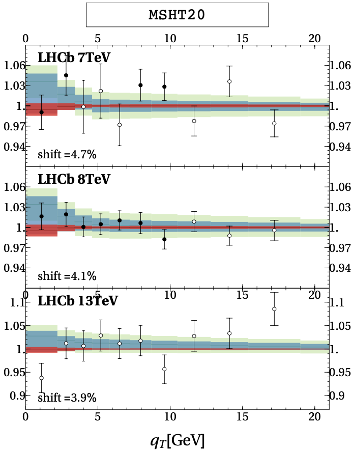
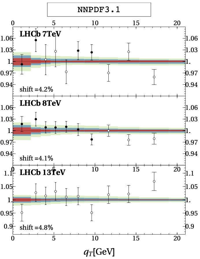
Figure 1: Example of the data description at high energy. Left panel: the ratio $d\sigma_{\rm{experiment}}/d\sigma_{\rm{theory}}$ for Z-boson production by the LHCb [26, 27, 28] experiment with two different sets of PDF. The red band is the EXP-uncertainty. The light-green band is the PDF-uncertainty. The blue band is the combined uncertainty. Only the filled bullets are included into the fit. More plots on Drell-Yan experimental results can be found in ref. [4].

References

References

- [1] J. Collins, Camb. Monogr. Part. Phys. Nucl. Phys. Cosmol. 32 (2011), 1-624
- [2] M. G. Echevarria, A. Idilbi and I. Scimemi, JHEP 07 (2012), 002
- [3] I. Scimemi and A. Vladimirov, JHEP 08 (2018), 003
- [4] M. Bury, F. Hautmann, S. Leal-Gomez, I. Scimemi, A. Vladimirov and P. Zurita, [arXiv:2201.07114 [hep-ph]].
-
[5]
artemide web-page: https://teorica.fis.ucm.es/artemide/;
artemide repository: https://github.com/VladimirovAlexey/artemide-public. For case https://github.com/SergioLealGomezTMD/artemide-development. - [6] I. Scimemi and A. Vladimirov, Eur. Phys. J. C 78 (2018) no.2, 89
- [7] R. D. Ball et al. [NNPDF], Nucl. Phys. B 809 (2009), 1-63 [erratum: Nucl. Phys. B 816 (2009), 293]
- [8] V. Bertone, I. Scimemi and A. Vladimirov, JHEP 06 (2019), 028
- [9] I. Scimemi and A. Vladimirov, JHEP 06 (2020), 137
- [10] F. Hautmann, I. Scimemi and A. Vladimirov, Phys. Lett. B 806 (2020), 135478.
- [11] T. Gehrmann, T. Luebbert and L. L. Yang, JHEP 06 (2014), 155.
- [12] M. G. Echevarria, I. Scimemi and A. Vladimirov, Phys. Rev. D 93 (2016) no.1, 011502 [erratum: Phys. Rev. D 94 (2016) no.9, 099904].
- [13] M. G. Echevarria, I. Scimemi and A. Vladimirov, Phys. Rev. D 93 (2016) no.5, 054004.
- [14] M. G. Echevarria, I. Scimemi and A. Vladimirov, JHEP 09 (2016), 004.
- [15] M. X. Luo, X. Wang, X. Xu, L. L. Yang, T. Z. Yang and H. X. Zhu, JHEP 10 (2019), 083.
- [16] M. x. Luo, T. Z. Yang, H. X. Zhu and Y. J. Zhu, Phys. Rev. Lett. 124 (2020) no.9, 092001.
- [17] M. x. Luo, T. Z. Yang, H. X. Zhu and Y. J. Zhu, JHEP 06 (2021), 115.
- [18] M. A. Ebert, B. Mistlberger and G. Vita, JHEP 09 (2020), 146.
- [19] A. A. Vladimirov, Phys. Rev. Lett. 118 (2017) no.6, 062001.
- [20] Y. Li and H. X. Zhu, Phys. Rev. Lett. 118 (2017) no.2, 022004.
- [21] T. J. Hou, J. Gao, T. J. Hobbs, K. Xie, S. Dulat, M. Guzzi, J. Huston, P. Nadolsky, J. Pumplin and C. Schmidt, et al. Phys. Rev. D 103 (2021) no.1, 014013.
- [22] H. Abramowicz et al. [H1 and ZEUS], Eur. Phys. J. C 75 (2015) no.12, 580.
- [23] S. Bailey, T. Cridge, L. A. Harland-Lang, A. D. Martin and R. S. Thorne, Eur. Phys. J. C 81 (2021) no.4, 341.
- [24] R. D. Ball et al. [NNPDF], Eur. Phys. J. C 77, no.10, 663 (2017).
- [25] A. Buckley, J. Ferrando, S. Lloyd, K. Nordström, B. Page, M. Rüfenacht, M. Schönherr and G. Watt, Eur. Phys. J. C 75 (2015), 132.
- [26] R. Aaij et al. [LHCb], JHEP 09 (2016), 136
- [27] R. Aaij et al. [LHCb], JHEP 08 (2015), 039.
- [28] R. Aaij et al. [LHCb], JHEP 01 (2016), 155.
- [29] V. Moos and A. Vladimirov, JHEP 12 (2020), 145.
- [30] [CMS], CMS-PAS-SMP-20-003.
- [31] R. Aaij et al. [LHCb], [arXiv:2112.07458 [hep-ex]].