Blueprint Separable Residual Network for Efficient Image Super-Resolution

Abstract

Recent advances in single image super-resolution (SISR) have achieved extraordinary performance, but the computational cost is too heavy to apply in edge devices. To alleviate this problem, many novel and effective solutions have been proposed. Convolutional neural network (CNN) with the attention mechanism has attracted increasing attention due to its efficiency and effectiveness. However, there is still redundancy in the convolution operation. In this paper, we propose Blueprint Separable Residual Network (BSRN) containing two efficient designs. One is the usage of blueprint separable convolution (BSConv), which takes place of the redundant convolution operation. The other is to enhance the model ability by introducing more effective attention modules. The experimental results show that BSRN achieves state-of-the-art performance among existing efficient SR methods. Moreover, a smaller variant of our model BSRN-S won the first place in model complexity track of NTIRE 2022 Efficient SR Challenge. The code is available at https://github.com/xiaom233/BSRN.

1 Introduction

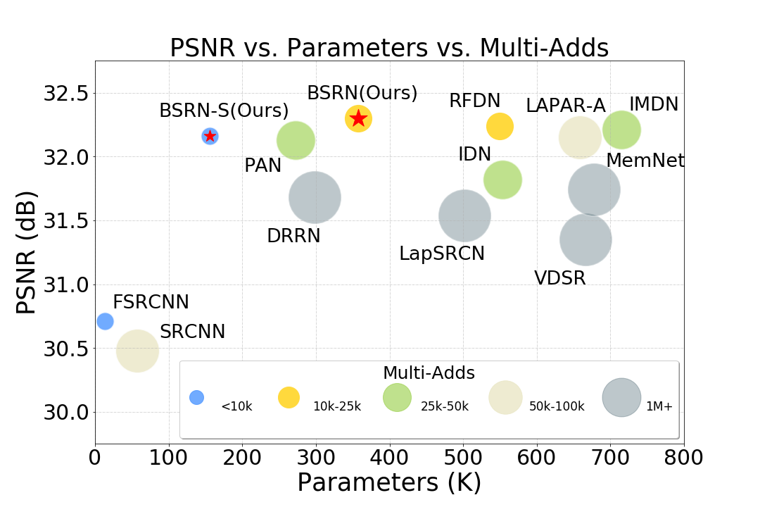
Figure 1: Performance and model complexity comparison on Set5 dataset for upscaling factor $\times 4$.

Single image super-resolution (SR) is a fundamental task in the computer vision field. It aims at reconstructing a visual-pleasing high-resolution (HR) image from the corresponding low-resolution (LR) observation. In recent years, the general paradigm has gradually shifted from model-based solutions to deep learning methods [9, 24, 36, 58, 4, 35]. These SR networks have greatly improved the quality of restored images. Their success can be partially attributed to the large model capacity and intensive computation. However, these properties could largely limit their application in real-world scenarios that prefer efficiency or require real-time implementation. Many lightweight SR networks have been proposed to address the inefficient issue. These approaches use different strategies to achieve high efficiency, including parameter sharing strategy [25, 50], cascading network with grouped convolution [2], information or feature distillation mechanisms [22, 21, 37] and attention mechanisms [60, 4]. While they have applied compact architectures and improved mapping efficiency, there still exists redundancy in convolution operations. We can build more efficient SR networks by reducing redundant computations and exploiting more effective modules.

In this paper, we propose a new lightweight SR network, namely Blueprint Separable Residual Network (BSRN), which improves the network’s efficiency from two perspectives — optimizing the convolutional operations and introducing effective attention modules. First, as the name suggests, BSRN reduces redundancies by using blueprint separation convolutions (BSConv) [11] to construct the basic building blocks. BSConv is an improved variant of the original depth-wise separable convolution (DSConv) [19], which better exploits intra-kernel correlations for an efficient separation [11]. Our work shows that BSConv is beneficial for efficient SR. Second, appropriate attention modules [21, 37, 60, 38] have been shown to improve the performance of efficient SR networks. Inspired by these works, we also introduce two effective attention modules, enhanced spatial attention (ESA) [38] and contrast-aware channel attention (CCA) [21], to enhance the model ability. The proposed BSRN method achieves state-of-the-art performance among existing efficiency-oriented SR networks, as shown in Fig. 1. We took a variant of our method BSRN-S to participate in the NTIRE 2022 Efficient SR Challenge and won first place in the model complexity track [34].

The main contributions of this paper are:

• We introduce BSConv to construct the basic building block and show its effectiveness for SR.

• We utilize two effective attention modules with limited extra computation to enhance the model ability.

• The proposed BSRN, which integrates BSConv and effective attention modules demonstrates superior performance for efficient SR.

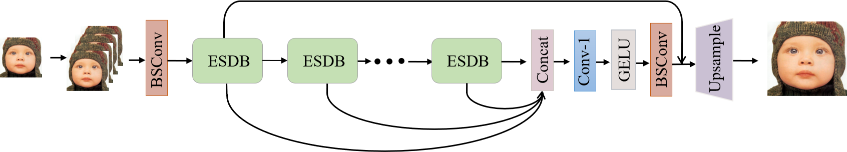
Figure 2: The architecture of Blueprint Separable Residual Network (BSRN).

2 Related Work

2.1 Deep Networks for SR

With the fast development of deep learning techniques, increasing remarkable progress has been made for the SR task. Since Dong et al. [9] proposed the pioneering work SRCNN with a three-layer convolutional neural network and significantly outperforms the conventional methods, a series of methods [24, 59, 59, 58, 35] have been proposed to improve the SR model. For example, Kim et al. [24] proved that a deeper network can get better performance by increasing the depth of the network to 20. Zhang et al. [59] introduced dense connection into the network to further enhance the representative ability of the model. [58] introduced the channel-wise attention mechanism to utilize the global statistics for better performance. Liang et al. [35] proposed a Transformer architecture for image restoration based on the Swin Transformer [39], which achieves a significant improvement and refreshes the state-of-the-art performance. Although the abovementioned approaches make great progress in performance, most of them bring high computational costs, which prompts researchers to develop more efficient methods for the SR task.

2.2 CNN Model Compression and Acceleration

During the past few years, tremendous progress has been made in the area of model compression and acceleration. In general, these techniques can be divided into four categories [5]: parameter pruning and quantization, low-rank factorization, knowledge distillation, and transferred/compact convolutional filters. For parameter pruning [14, 49, 29, 32] and quantization methods [52, 13, 6], they aim to explore the redundancy of the model architecture and try to remove or reduce the redundant parameters. The low-rank factorization approaches [45, 7] use matrix/tensor decomposition to estimate the more informative representation of the networks. Knowledge distillation methods[17, 27] aim to generate more compact student models from a larger network by learning the distributions of teacher models. The methods based on transferred/compact convolutional filters design [23, 19, 46, 57, 31, 18, 11] aim to devise special structural convolutional filters to reduce the model parameters and save storage/computation.

2.3 Efficient SR Models

Most of the current models for SR often introduce lots of computational costs when bringing performance improvements, which restricts the practical application of these methods. Thus, many works have been proposed to design more efficient models for the task [10, 25, 33, 50, 48, 2, 21, 60, 37, 54]. For instance, [10] directly used the original LR images as input instead of the pre-upsampled ones and placed a deconvolution at the end of the network to save computation. [2] uses group convolution to reduce the computation of the standard convolution. [22] proposed an information distillation network (IDN) that explicitly splits features and then processes them separately. [21] designed an information multi-distillation block that split features and refine them step by step to reduce the computation. [60] introduced pixel attention and self-calibrated convolution to use fewer parameters to achieve competitive performance. [37] proposed residual feature distillation block by improving the information distillation mechanism and won the championship of AIM 2020 Efficient SR Challenge [56].

3 Method

3.1 Network Architecture

The overall architecture of our method BSRN is shown in Fig. 2. It is inherited from the structure of RFDN [37], which is the champion solution of AIM 2020 Challenge on Efficient Super-Resolution. It consists of four stages: shallow feature extraction, deep feature extraction, multi-layer feature fusion and reconstruction. Let us denote $I_{LR}$ and $I_{SR}$ as the input and output image. In pre-processing, the input image is first replicated n times. Then we concatenate these images together as

$$I_{LR}^{n}=Concat_{n}(I_{LR}),$$ (1)

where $Concat(\cdot)$ denotes the concatenation operation along the channel dimension, and $n$ is the number of $I_{LR}$ to be concatenated. The next shallow feature extraction part maps the input image to a higher dimensional feature space as

$$F_{0}=H_{SF}(I_{LR}^{n}),$$ (2)

where $H_{SF}(\cdot)$ denotes the module of shallow feature extraction. To be specific, we use a BSConv [11] to achieve shallow feature extraction. The specific architecture of BSConv is depicted in Fig. 3 (g), which consists of a $1\times 1$ convolution and a depth-wise convolution. $F_{0}$ is then used for the deep feature extraction by a stack of ESDBs, which gradually refine the extracted features. This process can be formulated as

$$F_{k}=H_{k}(F_{k-1}),k=1,...,n,$$ (3)

where $H_{k}(\cdot)$ denotes the $k$-th ESDB. $F_{k-1}$ and $F_{k}$ represent the input feature and output feature of the $k$-th ESDB, respectively. To fully utilize features from all depths, features generated at different depths are fused and mapped by a $1\times 1$ convolution and a GELU[15] activation. Then, a BSConv is used to refine features. The multi-layer feature fusion is formulated as

$$F_{fused}=H_{fusion}(Concat(F_{1},...F_{k-1})),$$ (4)

where $H_{fusion}(\cdot)$ represents the fusion module and $F_{fused}$ is the aggregated feature. To take advantage of residual learning, a long skip connection is involved. The reconstruction stage is formulated as

$$I_{SR}=H_{BSRN}(I_{LR}^{i})=H_{rec}(F_{fusion}+F_{0}),$$ (5)

where $H_{rec}(\cdot)$ denotes the reconstruction module, which consists of a $3\times 3$ standard convolution layer and a pixel-shuffle operation [47]. $L_{1}$ loss function is exploited to optimize the model, which can be formulated as

$$L_{1}=\|I_{SR}-I_{HR}\|_{1}.$$ (6)

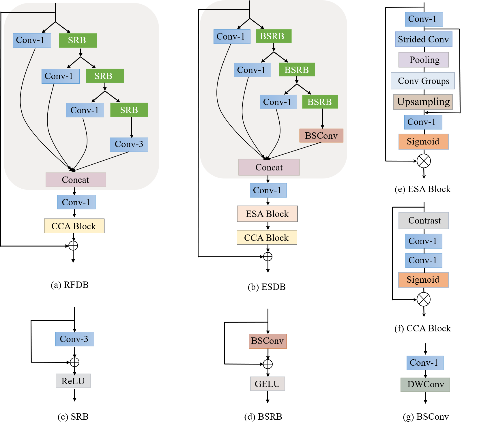
Figure 3: (a) The architecture of RFDB. (b) The architecture of the proposed ESDB. (c) The architecture of ESA block. (d) The architecture of channel weighting. (e) The architecture of SRB in RFDB. (f) The architecture of the proposed BSRB in ESDB. (g) The architecture of BSConv, consists of a $1\times 1$ convolution layer and a depth-wise convolution layer.

3.2 Efficient Separable Distillation Block

Inspired by the RFDB in RFDN [37], we design the efficient separable distillation block (ESDB) that is similar to RFDB in structure but more efficient. The overall architecture of ESDB is shown in Fig. 3 (b). An ESDB generally consists of 3 stages: feature distillation, feature condensation and feature enhancement. In the first stage, for an input feature $F_{in}$, the feature distillation can be formulated as

$$\begin{split}F_{distilled\_1},F_{coarse\_1}&=DL_{1}(F_{in}),RL_{1}(F_{in}),\\ F_{distilled\_2},F_{coarse\_2}&=DL_{2}(F_{coarse\_1}),RL_{2}(F_{coarse\_1}),\\ F_{distilled\_3},F_{coarse\_3}&=DL_{3}(F_{coarse\_2}),RL_{3}(F_{coarse\_2}),\\ F_{distilled\_4}&=DL_{4}(F_{coarse\_3}),\end{split}$$ (7)

where $DL$ denotes the distillation layer that generate distilled features, and $RL$ denotes the refinement layer that further refines the coarse feature step by step. In the feature condensation stage, the distilled features $F_{distilled\_1}$, $F_{distilled\_2}$, $F_{distilled\_3}$, $F_{distilled\_4}$ are concatenated together and then condensed by a $1\times 1$ convolution as

$$F_{condensed}=H_{linear}(Concat(F_{distilled\_1},...,F_{distilled\_4})),$$ (8)

where $F_{condensed}$ is the condensed feature, $H_{linear}(\cdot)$ denotes the $1\times 1$ convolution layer. For the last stage, to enhance the representational ability of the model while keeping efficiency, we introduce a lightweight enhanced spatial attention (ESA) block [38] and a contrast-aware channel attention (CCA) block [21] as

$$F_{enhanced}=H_{CCA}(H_{ESA}(F_{condensed})),$$ (9)

where $F_{enhanced}$ is the enhanced feature, $H_{ESA}(\cdot)$ and $H_{CCA}(\cdot)$ denote the ESA and CCA modules that have been shown to enhance the model ability effectively [38, 21] from the spatial and channel-wise perspective, respectively.

Table 1: Quantitative comparison of different convolution decomposition approaches. BSConvU is exploited in our method as BSConv.

Method	Params[K]	Multi-Adds[G]	Set5		Set14		B100		Urban100		Manga109
			PSNR	SSIM	PSNR	SSIM	PSNR	SSIM	PSNR	SSIM	PSNR	SSIM
RFDN	433K	23.9	32.04	0.8934	28.52	0.7799	27.53	0.7344	25.92	0.7810	30.30	0.9063
RFDN-DSConv	123K	6.9	31.95	0.8910	28.40	0.7772	27.45	0.7318	25.64	0.7726	29.84	0.9010
RFDN-BSConvS	122K	6.8	31.94	0.8917	28.44	0.7777	27.48	0.7322	25.70	0.7731	30.03	0.9027
RFDN-BSConvU	124K	6.8	31.99	0.8921	28.46	0.7783	27.47	0.7324	25.72	0.7742	29.99	0.9022

Table 2: Ablation study of ESA and CCA.

Method	Params[K]	Multi-Adds[G]	Set5		Set14		B100		Urban100		Manga109
			PSNR	SSIM	PSNR	SSIM	PSNR	SSIM	PSNR	SSIM	PSNR	SSIM
BSRN-woESA	320	18.2	32.14	0.8943	28.56	0.7807	27.56	0.7352	25.97	0.7816	30.39	0.9071
BSRN-woCCA	348	19.4	32.20	0.8947	28.65	0.7824	27.60	0.7368	26.05	0.7854	30.53	0.9087
BSRN	352	19.4	32.25	0.8956	28.62	0.7822	27.60	0.7367	26.10	0.7864	30.58	0.9093

Table 3: Quantitative comparison of different activation functions.

Method	DIV2K_val	Set5		Set14		B100		Urban100		Manga109
		PSNR	SSIM	PSNR	SSIM	PSNR	SSIM	PSNR	SSIM	PSNR	SSIM
ReLU	28.95	32.15	0.8943	28.59	0.7815	27.57	0.7358	26.02	0.7836	30.49	0.9082
LeakyReLU	28.97	32.24	0.8953	28.58	0.7817	27.58	0.7361	26.07	0.7854	30.55	0.9092
h-swish	28.99	32.22	0.8952	28.61	0.7825	27.59	0.7363	26.07	0.7851	30.50	0.9083
GELU	29.00	32.25	0.8956	28.62	0.7822	27.60	0.7367	26.10	0.7864	30.58	0.9093

Table 4: Quantitative comparison of two BSRN variants with RFDN. BSRN-1 has the same depth and width as RFDN, while BSRN-2 has similar computational complexity to RFDN.

Method	Params[K]	Multi-Adds[G]	Set5		Set14		B100		Urban100		Manga109
			PSNR	SSIM	PSNR	SSIM	PSNR	SSIM	PSNR	SSIM	PSNR	SSIM
RFDN	443	23.9	32.04	0.8934	28.52	0.7799	27.53	0.7344	25.92	0.7810	30.30	0.9063
BSRN-1	209	11.5	32.14	0.8942	28.57	0.7811	27.55	0.7352	25.95	0.7815	30.35	0.9068
BSRN-2	438	24.2	32.22	0.8954	28.62	0.7827	27.60	0.7369	26.08	0.7855	30.61	0.9096

Blueprint Shallow Residual Block (BSRB). A basic module of ESDB is BSRB, as shown in Fig. 3 (d), which consists of a BSConv, an identity connection and an activation unit. Specifically, we use GELU [16] as the activation function. BSConv factorizes a standard convolution into a point-wise $1\times 1$ convolution and a depth-wise convolution, as depicted in Fig. 3 (g). It is an inverse version of the depth-wise separable convolution (DSConv)[19]. [12] shows that BSConv performs better in many cases for efficient separation of the standard convolution, thus we exploit it in our model. For the activation unit, GELU [16] gradually becomes the first choice in recent works [8, 44, 39, 35], which can be seen as a smoother variant of ReLU. In our method, we also find that GELU performs better than the commonly used ReLU[43] and LeakyReLU[40].

Attention modules of ESA and CCA. Since the effectiveness of ESA and CCA has been proven [38, 21, 37], we introduce the two modules into our approach. The specific architecture of the ESA block is shown in Fig. 3 (f). It starts with a $1\times 1$ convolutional layer to reduce the channel dimensions of the input feature. Then the block uses a strided convolution and a strided max-pooling layer to reduce the spatial size. Following a group of convolutions to extract the feature, an interpolation-based up-sampling is performed to recover the spatial size. Note that the convolutions in our ESA are also BSConvs for better efficiency different from the original version [38]. Combined with a residual connection, the features are further processed by a $1\times 1$ convolutional layer to restore the channel size. Finally, the attention matrix is generated via a Sigmoid function and multiplied by the original input feature. A CCA block is added after the ESA block shown in Fig. 3 (f), which is an improved version of the channel attention module proposed for the SR task [21]. Different from the conventional channel attention calculated using the mean of each channel-wise feature, CCA utilizes the contrast information including the mean and the summation of standard deviation to calculate the channel attention weights.

4 Experiments

Table 5: Quantitative comparison with state-of-the-art methods on benchmark datasets. The best and second-best performance are in red and blue colors, respectively. ’Multi-Adds’ is calculated with a $1280\times 720$ GT image.

Method	Scale	Params[K]	Multi-Adds[G]	Set5	Set14	BSD100	Urban100	Manga109
				PSNR/SSIM	PSNR/SSIM	PSNR/SSIM	PSNR/SSIM	PSNR/SSIM
Bicubic	$\times 2$	-	-	33.66/0.9299	30.24/0.8688	29.56/0.8431	26.88/0.8403	30.80/0.9339
SRCNN[9]		8	52.7	36.66/0.9542	32.45/0.9067	31.36/0.8879	29.50/0.8946	35.60/0.9663
FSRCNN[10]		13	6.0	37.00/0.9558	32.63/0.9088	31.53/0.8920	29.88/0.9020	36.67/0.9710
VDSR[24]		666	612.6	37.53/0.9587	33.03/0.9124	31.90/0.8960	30.76/0.9140	37.22/0.9750
LapSRN[28]		251	29.9	37.52/0.9591	32.99/0.9124	31.80/0.8952	30.41/0.9103	37.27/0.9740
DRRN[50]		298	6,796.9	37.74/0.9591	33.23/0.9136	32.05/0.8973	31.23/0.9188	37.88/0.9749
MemNet[51]		678	2,662.4	37.78/0.9597	33.28/0.9142	32.08/0.8978	31.31/0.9195	37.72/0.9740
IDN[22]		553	124.6	37.83/0.9600	33.30/0.9148	32.08/0.8985	31.27/0.9196	38.01/0.9749
CARN[2]		1592	222.8	37.76/0.9590	33.52/0.9166	32.09/0.8978	31.92/0.9256	38.36/0.9765
IMDN[21]		694	158.8	38.00/0.9605	33.63/0.9177	32.19/0.8996	32.17/0.9283	38.88/0.9774
PAN[60]		261	70.5	38.00/0.9605	33.59/0.9181	32.18/0.8997	32.01/0.9273	38.70/0.9773
LAPAR-A[30]		548	171.0	38.01/0.9605	33.62/0.9183	32.19/0.8999	32.10/0.9283	38.67/0.9772
RFDN[37]		534	95.0	38.05/0.9606	33.68/0.9184	32.16/0.8994	32.12/0.9278	38.88/0.9773
BSRN(Ours)		332	73.0	38.10/0.9610	33.74/0.9193	32.24/0.9006	32.34/0.9303	39.14/0.9782
Bicubic	$\times 3$	-	-	30.39/0.8682	27.55/0.7742	27.21/0.7385	24.46/0.7349	26.95/0.8556
SRCNN[9]		8	52.7	32.75/0.9090	29.30/0.8215	28.41/0.7863	26.24/0.7989	30.48/0.9117
FSRCNN[10]		13	5.0	33.18/0.9140	29.37/0.8240	28.53/0.7910	26.43/0.8080	31.10/0.9210
VDSR[24]		666	612.6	33.66/0.9213	29.77/0.8314	28.82/0.7976	27.14/0.8279	32.01/0.9340
DRRN[50]		298	6,796,9	34.03/0.9244	29.96/0.8349	28.95/0.8004	27.53/0.8378	32.71/0.9379
MemNet[51]		678	2,662.4	34.09/0.9248	30.00/0.8350	28.96/0.8001	27.56/0.8376	32.51/0.9369
IDN[22]		553	56.3	34.11/0.9253	29.99/0.8354	28.95/0.8013	27.42/0.8359	32.71/0.9381
CARN[2]		1592	118.8	34.29/0.9255	30.29/0.8407	29.06/0.8034	28.06/0.8493	33.50/0.9440
IMDN[21]		703	71.5	34.36/0.9270	30.32/0.8417	29.09/0.8046	28.17/0.8519	33.61/0.9445
PAN[60]		261	39.0	34.40/0.9271	30.36/0.8423	29.11/0.8050	28.11/0.8511	33.61/0.9448
LAPAR-A[30]		544	114.0	34.36/0.9267	30.34/0.8421	29.11/0.8054	28.15/0.8523	33.51/0.9441
RFDN[37]		541	42.2	34.41/0.9273	30.34/0.8420	29.09/0.8050	28.21/0.8525	33.67/0.9449
BSRN(Ours)		340	33.3	34.46/0.9277	30.47/0.8449	29.18/0.8068	28.39/0.8567	34.05/0.9471
Bicubic	$\times 4$	-	-	28.42/0.8104	26.00/0.7027	25.96/0.6675	23.14/0.6577	24.89/0.7866
SRCNN[9]		8	52.7	30.48/0.8626	27.50/0.7513	26.90/0.7101	24.52/0.7221	27.58/0.8555
FSRCNN[10]		13	4.6	30.72/0.8660	27.61/0.7550	26.98/0.7150	24.62/0.7280	27.90/0.8610
VDSR[24]		666	612.6	31.35/0.8838	28.01/0.7674	27.29/0.7251	25.18/0.7524	28.83/0.8870
LapSRN[28]		813	149.4	31.54/0.8852	28.09/0.7700	27.32/0.7275	25.21/0.7562	29.09/0.8900
DRRN[50]		298	6,796.9	31.68/0.8888	28.21/0.7720	27.38/0.7284	25.44/0.7638	29.45/0.8946
MemNet[51]		678	2,662.4	31.74/0.8893	28.26/0.7723	27.40/0.7281	25.50/0.7630	29.42/0.8942
IDN[22]		553	32.3	31.82/0.8903	28.25/0.7730	27.41/0.7297	25.41/0.7632	29.41/0.8942
CARN[2]		1592	90.9	32.13/0.8937	28.60/0.7806	27.58/0.7349	26.07/0.7837	30.47/0.9084
IMDN[21]		715	40.9	32.21/0.8948	28.58/0.7811	27.56/0.7353	26.04/0.7838	30.45/0.9075
PAN[60]		272	28.2	32.13/0.8948	28.61/0.7822	27.59/0.7363	26.11/0.7854	30.51/0.9095
LAPAR-A[30]		659	94.0	32.15/0.8944	28.61/0.7818	27.61/0.7366	26.14/0.7871	30.42/0.9074
RFDN[37]		550	23.9	32.24/0.8952	28.61/0.7819	27.57/0.7360	26.11/0.7858	30.58/0.9089
BSRN-S(Ours)		156	8.3	32.16/0.8949	28.62/0.7823	27.58/0.7365	26.08/0.7849	30.53/0.9089
BSRN(Ours)		352	19.4	32.35/0.8966	28.73/0.7847	27.65/0.7387	26.27/0.7908	30.84/0.9123

4.1 Experimental Setup

Datasets and Metrics. The training images consist of 2650 images from Flickr2K[36] and 800 images from DIV2K[1]. We use the five standard benchmark datasets of Set5[3], Set14[55], B100[41], Urban100[20], and Manga109[42] to evaluate the performance of different approaches. The average peak signal to noise ratio (PSNR) and the structural similarity[53] (SSIM) on the Y channel (i.e., luminance) are exploited as the evaluation metrics.

Implementation details of BSRN. The proposed BSRN consists of 8 ESDBs and the number of channels is set to 64. The kernel size of all depth-wise convolutions is set to 3. Data augmentation methods of random rotation by 90^∘, 180^∘, 270^∘ and flipping horizontally are utilized. The mini-batch size is set to 64 and the patch size of each LR input is set to $48\times 48$. The model is trained by Adam optimizer[26] with $\beta_{1}=0.9,\beta_{2}=0.999$. The initial learning rate is set to $1\times 10^{-3}$ with cosine learning rate decay. $L_{1}$ loss is used to optimize the model for total $1\times 10^{6}$ iterations. We use Pytorch to implement our model on two GeForce RTX 3090 GPUs and the training process costs about 30 hours.

Implementation details of BSRN-S for NTIRE2022 Challenge. BSRN-S is a small variant of BSRN designed for the challenge, which requires the participants to devise an efficient network while maintaining PSNR of 29.00dB on DIV2K validation dataset. Specifically, we reduce the number of ESDBs to 5 and the number of features to 48. The CCA block is replaced with learnable channel-wise weights. During the training process, the input patch size is set to $64\times 64$ and the mini-batch is set to 256. The number of training iterations is increased to $1.5\times 10^{6}$ and four GeForce RTX 2080Ti GPUs are used for training.

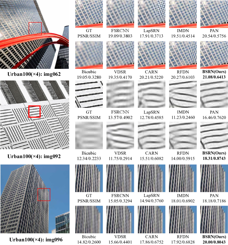
Figure 4: Visual comparison of BSRN with the state-of-the-art methods on $\times$4 SR.

Table 6: Results of NTIRE 2022 Efficient Super-Resolution Sub-Track 1: Model Complexity.

Team	Val PSNR	Test PSNR	Params[M]	FLOPs[G]	Acts[M]	Mem[M]	Runtime[ms]
XPixel (Ours)	29.01	28.69	0.156	9.496	65.76	729.94	140.47
NJUST_ESR	28.96	28.68	0.176	8.73	160.43	1346.74	164.8
HisenseResearch	29.00	28.72	0.242	14.51	151.36	861.84	47.75
NEESR	29.01	28.71	0.272	16.86	79.59	575.99	29.97
NKU-ESR	29.00	28.66	0.276	16.73	111.12	662.51	34.81
RFDN AIM2020 Winner	29.04	28.75	0.433	27.1	112.03	788.13	41.97

4.2 Ablation Study

In this section, we first present the effects of different convolution decomposition methods. Then we demonstrate the effectiveness of the two attention modules and compare the effects of different activation functions. Finally, we further show the effectiveness of the proposed architecture.

Effects of different convolution decompositions. We conduct experiments to show the effects of different ways of convolution decomposition based on RFDN. The experimental results are presented in Tab. 1. DSConv represents the original depth-wise separable convolution [19]. BSConvU and BSConvS represent the two variants of BSConv proposed in [12]. We can observe that apparent performance drops appear with significant computation decreases when performing convolution decompositions. Among the three decomposition strategies, BSConvU performs the best, thus we choose to use it in our model.

Effectiveness of ESA and CCA. We also conduct the ablation study to validate the effectiveness of the two attention modules of ESA and CCA, as depicted in Tab. 2. With about 9% drop in parameters, an obvious performance drop appears for BSRN without ESA. Compared to BSRN without CCA, the complete BSRN obtains performance gains of 0.5dB on Set5, Urban100 and Manga109 datasets. The results demonstrate that ESA and CCA can effectively enhance the model capacity.

Exploration of different activation functions. Most of the previous SR networks adopt ReLU [43] or LeakyReLU [40] as the activation function. However, GELU [15] is gradually becoming the mainstream choice in recent works. [18] investigates the effects of different activation functions in an efficient model MobileNet V3 and proposes a new activation function h-swish. Therefore, we also investigate various activation functions to explore the best choice for our method. The results in Tab. 3 show that different activation functions can obviously affect the performance of the model. Among these activation functions, GELU obtains a remarkable performance gain, especially on the Urban100 dataset. Thus, we choose GELU as the activation function in our model.

Effectiveness of the proposed architecture. We design two variants of BSRN to demonstrate the effectiveness of the proposed architecture. We set the depth and width of BSRN the same as the original RFDN for BSRN-1 and then enlarge the model capacity to the similar computations to RFDN for BSRN-2. Note that we train the compared models under the same training settings for a fair comparison. As shown in Tab. 4, we can observe that BSRN-1 outperforms RFDN with less computation. In addition, BSRN-2 obtains a significant performance gain compared to RFDN, especially on the Manga109 dataset. The experimental results show the superiority of the proposed architecture.

4.3 Comparison with State-of-the-art Methods

We compare the proposed BSRN with state-of-the-art lightweight SR approaches, including SRCNN[9], FSRCNN[10], VDSR[24], LapSRN[28], DRRN[50], MemNet[51], IDN[22], CARN[2], IMDN[21], PAN[60], LAPAR-A[30], RFDN[37]. Tab. 5 shows the quantitative comparison results for different upscale factors. We also provide the number of parameters and Multi-Adds calculated on the $1280\times 720$ output. Compared to other lightweight SR methods, our BSRN achieves the best performance with only 332K-352K parameters and almost the fewest Multi-Adds. Our solution for NTIRE Challenge, BSRN-S, also obtains competitive performance with only 156K parameters and 8.3G Multi-Adds on $\times$4 SR. The qualitative comparison is demonstrated in Fig. 4 and our approach can also obtain the best visual quality compared to the state-of-the-art methods.

4.4 BSRN-S for NTIRE2022 Challenge

Our BSRN-S won the first place in the NTIRE2022 Efficient Super-Resolution Challenge Sub-Track 1: Model Complexity, for which the summed rank of the number of parameters and FLOPs are utilized for the final ranking. The results are shown in Tab. 6. Note that we use different settings to train the model for the challenge that is presented in Sec. 4.1. For the specific metrics in the table, ’Val PSNR’ and ’Test PSNR’ are PSNR results tested on the DIV2K validation and test sets. Compared to other competing solutions, our method has the least number of parameters and the second-fewest FLOPs. For the average runtime, it is related to the optimization of the code and the calculation of the specific testing platform for different operators. After optimization, BSRN-S-opt obtains similar runtime to IMDN and RFDN on the same GPU shown in Tab. 7. However, since it is unfriendly for GPU to calculate depth-wise convolution, the runtime of our approach is relatively larger.

Table 7: Comparison of computational cost.

Team	Params[K]	Multi-Adds[G]	Mem[M]	Runtime[ms]
MSRResNet	1517.57	166.36	598.55	70.83
IMDN	893.94	58.53	120.17	25.32
RFDN	433.45	27.10	201.59	26.53
BSRN-S(ours)	156.05	8.35	184.57	36.51
BSRN-S-opt(ours)	156.05	8.35	184.57	26.81

5 Conclusions

In this paper, we propose a lightweight network for single image super-resolution called the blueprint separable residual network (BSRN). The design of BSRN is inspired by the residual feature distillation network (RFDN) and the blueprint separable convolution (BSConv). We adopt the similar architecture of RFDN but introduce a more efficient blueprint shallow residual block (BSRB) by replacing the standard convolution with BSConv in the shallow residual block (SRB) in RFDN. Moreover, we use the effective ECA block and CCA block to enhance the representative ability of the model. Extensive experiments show that our method achieves the best performance with fewer parameters and Multi-Adds compared to the state-of-the-art efficient SR methods. Besides, our solution won first place in the model complexity track of the NTIRE 2022 efficient super-resolution challenge.

Acknowledgements.

This work is partially supported by the National Natural Science Foundation of China (61906184), the Joint Lab of CAS-HK, the Shenzhen Research Program(RCJC20200714114557087), the Shanghai Committee of Science and Technology, China (Grant No. 21DZ1100100).

References

- [1] Eirikur Agustsson and Radu Timofte. Ntire 2017 challenge on single image super-resolution: Dataset and study. In Proceedings of the IEEE conference on computer vision and pattern recognition workshops, pages 126–135, 2017.
- [2] Namhyuk Ahn, Byungkon Kang, and Kyung-Ah Sohn. Fast, accurate, and lightweight super-resolution with cascading residual network. In Proceedings of the European conference on computer vision (ECCV), pages 252–268, 2018.
- [3] Marco Bevilacqua, Aline Roumy, Christine Guillemot, and Marie Line Alberi-Morel. Low-complexity single-image super-resolution based on nonnegative neighbor embedding. 2012.
- [4] Haoyu Chen, Jinjin Gu, and Zhi Zhang. Attention in attention network for image super-resolution. arXiv preprint arXiv:2104.09497, 2021.
- [5] Yu Cheng, Duo Wang, Pan Zhou, and Tao Zhang. A survey of model compression and acceleration for deep neural networks. arXiv preprint arXiv:1710.09282, 2017.
- [6] Matthieu Courbariaux, Yoshua Bengio, and Jean-Pierre David. Binaryconnect: Training deep neural networks with binary weights during propagations. Advances in neural information processing systems, 28, 2015.
- [7] Misha Denil, Babak Shakibi, Laurent Dinh, Marc’Aurelio Ranzato, and Nando De Freitas. Predicting parameters in deep learning. Advances in neural information processing systems, 26, 2013.
- [8] Jacob Devlin, Ming-Wei Chang, Kenton Lee, and Kristina Toutanova. Bert: Pre-training of deep bidirectional transformers for language understanding. arXiv preprint arXiv:1810.04805, 2018.
- [9] Chao Dong, Chen Change Loy, Kaiming He, and Xiaoou Tang. Learning a deep convolutional network for image super-resolution. In European conference on computer vision, pages 184–199. Springer, 2014.
- [10] Chao Dong, Chen Change Loy, and Xiaoou Tang. Accelerating the super-resolution convolutional neural network. In European conference on computer vision, pages 391–407. Springer, 2016.
- [11] Daniel Haase and Manuel Amthor. Rethinking depthwise separable convolutions: How intra-kernel correlations lead to improved mobilenets. In Proceedings of the IEEE/CVF Conference on Computer Vision and Pattern Recognition, pages 14600–14609, 2020.
- [12] Daniel Haase and Manuel Amthor. Rethinking depthwise separable convolutions: How intra-kernel correlations lead to improved mobilenets. In Proceedings of the IEEE/CVF Conference on Computer Vision and Pattern Recognition, pages 14600–14609, 2020.
- [13] Song Han, Huizi Mao, and William J Dally. Deep compression: Compressing deep neural networks with pruning, trained quantization and huffman coding. arXiv preprint arXiv:1510.00149, 2015.
- [14] Stephen Hanson and Lorien Pratt. Comparing biases for minimal network construction with back-propagation. Advances in neural information processing systems, 1, 1988.
- [15] Dan Hendrycks and Kevin Gimpel. Gaussian error linear units (gelus). arXiv preprint arXiv:1606.08415, 2016.
- [16] Dan Hendrycks and Kevin Gimpel. Gaussian error linear units (gelus). arXiv preprint arXiv:1606.08415, 2016.
- [17] Geoffrey Hinton, Oriol Vinyals, and Jeffrey Dean. Distilling the knowledge in a neural network. In NIPS Deep Learning and Representation Learning Workshop, 2015.
- [18] Andrew Howard, Mark Sandler, Grace Chu, Liang-Chieh Chen, Bo Chen, Mingxing Tan, Weijun Wang, Yukun Zhu, Ruoming Pang, Vijay Vasudevan, et al. Searching for mobilenetv3. In Proceedings of the IEEE/CVF International Conference on Computer Vision, pages 1314–1324, 2019.
- [19] Andrew G Howard, Menglong Zhu, Bo Chen, Dmitry Kalenichenko, Weijun Wang, Tobias Weyand, Marco Andreetto, and Hartwig Adam. Mobilenets: Efficient convolutional neural networks for mobile vision applications. arXiv preprint arXiv:1704.04861, 2017.
- [20] Jia-Bin Huang, Abhishek Singh, and Narendra Ahuja. Single image super-resolution from transformed self-exemplars. In Proceedings of the IEEE conference on computer vision and pattern recognition, pages 5197–5206, 2015.
- [21] Zheng Hui, Xinbo Gao, Yunchu Yang, and Xiumei Wang. Lightweight image super-resolution with information multi-distillation network. In Proceedings of the 27th acm international conference on multimedia, pages 2024–2032, 2019.
- [22] Zheng Hui, Xiumei Wang, and Xinbo Gao. Fast and accurate single image super-resolution via information distillation network. In Proceedings of the IEEE conference on computer vision and pattern recognition, pages 723–731, 2018.
- [23] Forrest N Iandola, Song Han, Matthew W Moskewicz, Khalid Ashraf, William J Dally, and Kurt Keutzer. Squeezenet: Alexnet-level accuracy with 50x fewer parameters and¡ 0.5 mb model size. arXiv preprint arXiv:1602.07360, 2016.
- [24] Jiwon Kim, Jung Kwon Lee, and Kyoung Mu Lee. Accurate image super-resolution using very deep convolutional networks. In Proceedings of the IEEE conference on computer vision and pattern recognition, pages 1646–1654, 2016.
- [25] Jiwon Kim, Jung Kwon Lee, and Kyoung Mu Lee. Deeply-recursive convolutional network for image super-resolution. In Proceedings of the IEEE conference on computer vision and pattern recognition, pages 1637–1645, 2016.
- [26] Diederik P Kingma and Jimmy Ba. Adam: A method for stochastic optimization. arXiv preprint arXiv:1412.6980, 2014.
- [27] Anoop Korattikara Balan, Vivek Rathod, Kevin P Murphy, and Max Welling. Bayesian dark knowledge. Advances in Neural Information Processing Systems, 28, 2015.
- [28] Wei-Sheng Lai, Jia-Bin Huang, Narendra Ahuja, and Ming-Hsuan Yang. Deep laplacian pyramid networks for fast and accurate super-resolution. In Proceedings of the IEEE conference on computer vision and pattern recognition, pages 624–632, 2017.
- [29] Vadim Lebedev and Victor Lempitsky. Fast convnets using group-wise brain damage. In Proceedings of the IEEE Conference on Computer Vision and Pattern Recognition, pages 2554–2564, 2016.
- [30] Wenbo Li, Kun Zhou, Lu Qi, Nianjuan Jiang, Jiangbo Lu, and Jiaya Jia. Lapar: Linearly-assembled pixel-adaptive regression network for single image super-resolution and beyond. Advances in Neural Information Processing Systems, 33:20343–20355, 2020.
- [31] Yawei Li, Shuhang Gu, Luc Van Gool, and Radu Timofte. Learning filter basis for convolutional neural network compression. In Proceedings of the IEEE/CVF International Conference on Computer Vision, pages 5623–5632, 2019.
- [32] Yawei Li, Shuhang Gu, Kai Zhang, Luc Van Gool, and Radu Timofte. Dhp: Differentiable meta pruning via hypernetworks. In European Conference on Computer Vision, pages 608–624. Springer, 2020.
- [33] Yawei Li, Wen Li, Martin Danelljan, Kai Zhang, Shuhang Gu, Luc Van Gool, and Radu Timofte. The heterogeneity hypothesis: Finding layer-wise differentiated network architectures. In Proceedings of the IEEE/CVF Conference on Computer Vision and Pattern Recognition, pages 2144–2153, 2021.
- [34] Yawei Li, Kai Zhang, Luc Van Gool, Radu Timofte, et al. Ntire 2022 challenge on efficient super-resolution: Methods and results. In IEEE Conference on Computer Vision and Pattern Recognition Workshops, 2022.
- [35] Jingyun Liang, Jiezhang Cao, Guolei Sun, Kai Zhang, Luc Van Gool, and Radu Timofte. Swinir: Image restoration using swin transformer. In Proceedings of the IEEE/CVF International Conference on Computer Vision, pages 1833–1844, 2021.
- [36] Bee Lim, Sanghyun Son, Heewon Kim, Seungjun Nah, and Kyoung Mu Lee. Enhanced deep residual networks for single image super-resolution. In Proceedings of the IEEE conference on computer vision and pattern recognition workshops, pages 136–144, 2017.
- [37] Jie Liu, Jie Tang, and Gangshan Wu. Residual feature distillation network for lightweight image super-resolution. In European Conference on Computer Vision, pages 41–55. Springer, 2020.
- [38] Jie Liu, Wenjie Zhang, Yuting Tang, Jie Tang, and Gangshan Wu. Residual feature aggregation network for image super-resolution. In Proceedings of the IEEE/CVF conference on computer vision and pattern recognition, pages 2359–2368, 2020.
- [39] Ze Liu, Yutong Lin, Yue Cao, Han Hu, Yixuan Wei, Zheng Zhang, Stephen Lin, and Baining Guo. Swin transformer: Hierarchical vision transformer using shifted windows. In Proceedings of the IEEE/CVF International Conference on Computer Vision, pages 10012–10022, 2021.
- [40] Andrew L Maas, Awni Y Hannun, Andrew Y Ng, et al. Rectifier nonlinearities improve neural network acoustic models. In Proc. icml, volume 30, page 3. Citeseer, 2013.
- [41] David Martin, Charless Fowlkes, Doron Tal, and Jitendra Malik. A database of human segmented natural images and its application to evaluating segmentation algorithms and measuring ecological statistics. In Proceedings Eighth IEEE International Conference on Computer Vision. ICCV 2001, volume 2, pages 416–423. IEEE, 2001.
- [42] Yusuke Matsui, Kota Ito, Yuji Aramaki, Azuma Fujimoto, Toru Ogawa, Toshihiko Yamasaki, and Kiyoharu Aizawa. Sketch-based manga retrieval using manga109 dataset. Multimedia Tools and Applications, 76(20):21811–21838, 2017.
- [43] Vinod Nair and Geoffrey E Hinton. Rectified linear units improve restricted boltzmann machines. In Icml, 2010.
- [44] Alec Radford, Jeffrey Wu, Rewon Child, David Luan, Dario Amodei, Ilya Sutskever, et al. Language models are unsupervised multitask learners. OpenAI blog, 1(8):9, 2019.
- [45] Roberto Rigamonti, Amos Sironi, Vincent Lepetit, and Pascal Fua. Learning separable filters. In Proceedings of the IEEE conference on computer vision and pattern recognition, pages 2754–2761, 2013.
- [46] Mark Sandler, Andrew Howard, Menglong Zhu, Andrey Zhmoginov, and Liang-Chieh Chen. Mobilenetv2: Inverted residuals and linear bottlenecks. In Proceedings of the IEEE Conference on Computer Vision and Pattern Recognition (CVPR), June 2018.
- [47] Wenzhe Shi, Jose Caballero, Ferenc Huszár, Johannes Totz, Andrew P Aitken, Rob Bishop, Daniel Rueckert, and Zehan Wang. Real-time single image and video super-resolution using an efficient sub-pixel convolutional neural network. In Proceedings of the IEEE conference on computer vision and pattern recognition, pages 1874–1883, 2016.
- [48] Dehua Song, Chang Xu, Xu Jia, Yiyi Chen, Chunjing Xu, and Yunhe Wang. Efficient residual dense block search for image super-resolution. In Proceedings of the AAAI Conference on Artificial Intelligence, volume 34, pages 12007–12014, 2020.
- [49] Suraj Srinivas and R Venkatesh Babu. Data-free parameter pruning for deep neural networks. arXiv preprint arXiv:1507.06149, 2015.
- [50] Ying Tai, Jian Yang, and Xiaoming Liu. Image super-resolution via deep recursive residual network. In Proceedings of the IEEE conference on computer vision and pattern recognition, pages 3147–3155, 2017.
- [51] Ying Tai, Jian Yang, Xiaoming Liu, and Chunyan Xu. Memnet: A persistent memory network for image restoration. In Proceedings of the IEEE international conference on computer vision, pages 4539–4547, 2017.
- [52] Vincent Vanhoucke, Andrew Senior, and Mark Z Mao. Improving the speed of neural networks on cpus. 2011.
- [53] Zhou Wang, Alan C Bovik, Hamid R Sheikh, and Eero P Simoncelli. Image quality assessment: from error visibility to structural similarity. IEEE transactions on image processing, 13(4):600–612, 2004.
- [54] Yan Wu, Zhiwu Huang, Suryansh Kumar, Rhea Sanjay Sukthanker, Radu Timofte, and Luc Van Gool. Trilevel neural architecture search for efficient single image super-resolution. arXiv preprint arXiv:2101.06658, 2021.
- [55] Roman Zeyde, Michael Elad, and Matan Protter. On single image scale-up using sparse-representations. In International conference on curves and surfaces, pages 711–730. Springer, 2010.
- [56] Kai Zhang, Martin Danelljan, Yawei Li, Radu Timofte, Jie Liu, Jie Tang, Gangshan Wu, Yu Zhu, Xiangyu He, Wenjie Xu, et al. Aim 2020 challenge on efficient super-resolution: Methods and results. In European Conference on Computer Vision, pages 5–40. Springer, 2020.
- [57] Xiangyu Zhang, Xinyu Zhou, Mengxiao Lin, and Jian Sun. Shufflenet: An extremely efficient convolutional neural network for mobile devices. In Proceedings of the IEEE conference on computer vision and pattern recognition, pages 6848–6856, 2018.
- [58] Yulun Zhang, Kunpeng Li, Kai Li, Lichen Wang, Bineng Zhong, and Yun Fu. Image super-resolution using very deep residual channel attention networks. In Proceedings of the European conference on computer vision (ECCV), pages 286–301, 2018.
- [59] Yulun Zhang, Yapeng Tian, Yu Kong, Bineng Zhong, and Yun Fu. Residual dense network for image super-resolution. In Proceedings of the IEEE conference on computer vision and pattern recognition, pages 2472–2481, 2018.
- [60] Hengyuan Zhao, Xiangtao Kong, Jingwen He, Yu Qiao, and Chao Dong. Efficient image super-resolution using pixel attention. In European Conference on Computer Vision, pages 56–72. Springer, 2020.