Parametrization and Estimation of High-Rank Line-of-Sight MIMO Channels with Reflected Paths

Abstract

High-rank line-of-sight (LOS) MIMO systems have attracted considerable attention for millimeter wave and THz communications. The small wavelengths in these frequencies enable spatial multiplexing with massive data rates at long distances. Such systems are also being considered for multi-path non-LOS (NLOS) environments. In these scenarios, standard channel models based on plane waves cannot capture the curvature of each wave front necessary to model spatial multiplexing. This work presents a novel and simple multi-path wireless channel parametrization where each path is replaced by a LOS path with a reflected image source. The model is fully valid for all paths with specular planar reflections, and captures the spherical nature of each wave front. Importantly, it is shown that the model uses only two additional parameters relative to the standard plane wave model. Moreover, the parameters can be easily captured in standard ray tracing. The accuracy of the approach is demonstrated on detailed ray tracing simulations at $28\text{\,}\mathrm{G}\mathrm{H}\mathrm{z}$ and $140\text{\,}\mathrm{G}\mathrm{H}\mathrm{z}$ in a dense urban area.

I Introduction

Line-of-sight (LOS) multi-input multi-output (MIMO) systems [1, 2, 3, 4] have emerged as a valuable technology for the millimeter wave (mmWave) and terahertz (THz) frequencies. The concept is to operate communication links at a transmitter-receiver (TX-RX) separation, $R$, less than the so-called Rayleigh distance,

$$R<R_{\rm rayleigh}\approx\frac{2D^{2}}{\lambda},$$ (1)

where $D$ is the total aperture of the TX and RX arrays and $\lambda$ is the wavelength. In this regime, links can support multiple spatial streams even with a single LOS path [5]. LOS MIMO is particularly valuable in the mmWave and THz frequencies, where the wavelength $\lambda$ is small and hence the Rayleigh distance — which sets the maximum range of such systems — can be large with moderate size apertures $D$. For example, at $140\text{\,}\mathrm{G}\mathrm{H}\mathrm{z}$ carrier frequency with an aperture of $D=$ $1\text{\,}\mathrm{m}$, the Rayleigh distance is $R_{\rm rayleigh}\approx$ $930\text{\,}\mathrm{m}$ enabling long range communication while remaining below the Rayleigh distance.

Indeed, there have been several demonstrations in the $60\text{\,}\mathrm{G}\mathrm{H}\mathrm{z}$ mmWave bands [6]. Also, with the advancement of communication systems in the THz and sub-THz bands [7], there has been growing interest in high-rank LOS MIMO in higher frequencies as well [8] – see, for example, some recent work at $140\text{\,}\mathrm{G}\mathrm{H}\mathrm{z}$ [9, 10].

Many applications for such LOS MIMO systems are envisioned as operating in NLOS settings. For example, in mid-haul and backhaul applications – a key target application for sub-THz systems [10, 11, 12] – NLOS paths may be present from ground clutter when serving street-level radio units. In this work, we will use the term wide aperture MIMO, instead of LOS MIMO, since we are also interested in cases where the systems operate in such NLOS settings.

Evaluating wide aperture systems in NLOS environments requires accurate channel models to describe multi-path propagation. Conventional statistical multipath models, such as QuaDRiGA [13] and 3GPP [14], describe each path as a propagating plane wave with a gain, delay, and directions of arrival and departure. Under this standard plane wave approximation (PWA), the MIMO channel response can be computed for any array geometries at the TX and RX [15]. However, the PWA model is not valid when the TX-RX separation is below the Rayleigh distance (i.e., not in the far-field), since the curvature of each wavefront becomes important. While spherical wave models are well-understood for single LOS path channels [16], there are currently few techniques to model them in NLOS multi-path settings.

Figure 1: The proposed reflection model replaces each reflected path with a LOS path with a mirror image source. The spherical wave from this source can then be easily modeled for arbitrarily wide aperture arrays.

In this work, we present a simple parametrization for multipath channels that capture the full spherical nature of each wavefront. The model is valid for both LOS paths as well as NLOS paths arising from arbitrary numbers of specular reflections from flat surfaces (i.e., no curvature). The main concept is that, in such environments, each NLOS path can be replaced by a LOS path where the TX location is replaced by a virtual image source from the reflection on the source – See Fig. 1. This idea is the same concept that underlies the method of images in ray tracing [17]. See, also [18] for modeling reflections in the near field. Our main contribution here shows that the propagation from each such image can be parametrized by two additional parameters relative to the plane wave model. We call the parametrization the reflection model, or RM.

In addition, we show how these parameters can be extracted for site-specific evaluations via ray tracing. Analyzing wide aperture systems with ray tracing typically requires running the simulations between each transmitter and receiver element pair, which can be computationally expensive when the number of elements is large. In addition, the ray tracing must be repeated for different antenna geometries or orientations, making site planning and capacity evaluation time-consuming. In contrast, we show how the full parameters for the RM can be computed from ray tracing a single ray tracing simulation near the array centers. As an illustration, we show an example application of using the RM model to estimate the MIMO capacity in a point-to-point link with dramatically lower ray tracing simulation time than would be required exhaustive ray tracing.

Prior Work

As stated above, most current industry models, such as [13] and [14], use a plane wave approximation, which is only valid in the far-field. Obtaining the exact near-field behavior, generally requires performing ray tracing between each TX and RX element. In this sequel, we will call this method exhaustive ray tracing. While accurate, exhaustive ray tracing is computationally expensive. The closest related line of work to finding computationally simpler models can be found in the recent papers [19, 20, 21, 4]. These works consider near field channels from point scatterers close to the receiver. In contrast, the present paper considers reflections from surfaces in the near-field of the transmitter or receiver. A key difference with surfaces is that the point of reflection is different for different TX and RX element positions.

II Plane Wave Approximations for Multi-Path Channels

We begin by reviewing the standard plane wave multi-path channel models using the perspective in [16]. Consider a wireless channel from a TX locations ${\boldsymbol{x}}^{t}\in{\mathcal{A}}^{t}$ to RX locations ${\boldsymbol{x}}^{r}\in{\mathcal{A}}^{r}$, where ${\mathcal{A}}^{t}$ and ${\mathcal{A}}^{r}\subset{\mathbb{R}}^{p}$ are some regions that can contain the elements in the TX and RX arrays. We focus on so-called 3D models with $p=3$, although similar results can be derived for $p=2$. We assume the channel is described by a set of $L$ discrete paths representing the routes of propagation from the TX to RX locations. In this case, the channel frequency response at a frequency $f$ from a transmit location ${\boldsymbol{x}}^{t}$ to a receive location ${\boldsymbol{x}}^{r}$ is given by:

$$H(f)=\sum_{\ell=1}^{L}g_{\ell}\exp\left(-\frac{j2\pi f}{c}d_{\ell}({\boldsymbol{x}}^{r},{\boldsymbol{x}}^{t})\right),$$ (2)

where, for each path $\ell=1,\ldots,L$, $g_{\ell}$ is a complex nominal channel gain (assumed to be approximately constant over the region), $d_{\ell}({\boldsymbol{x}}^{r},{\boldsymbol{x}}^{t})$ is the propagation distance along the path from ${\boldsymbol{x}}^{t}$ to ${\boldsymbol{x}}^{r}$, and $c$ is the speed of light [15]. We will call $d_{\ell}({\boldsymbol{x}}^{r},{\boldsymbol{x}}^{t})$ the path distance function for path $\ell$.

Describing the gain $g_{\ell}$ and path distance function $d_{\ell}(\cdot)$ for each path is sufficient to compute the response for arbitrary TX and RX arrays in multi-path environments. For example, suppose that the TX array has $N_{\rm tx}$ elements at locations $x^{t}_{n}\in{\mathcal{A}}^{t}$, $n=1,\ldots,N_{\rm tx}$ and the RX array has elements at locations $x^{r}_{m}\in{\mathcal{A}}^{r}$, $m=1,\ldots,N_{\rm rx}$. Then, the MIMO frequency response is the matrix with coefficients

$$H_{mn}(f)=\sum_{\ell=1}^{L}g_{\ell}\exp\left(-\frac{j2\pi f}{c}d_{\ell}({\boldsymbol{x}}^{r}_{m},{\boldsymbol{x}}^{t}_{n})\right).$$ (3)

Hence, if we can find the gain $g_{\ell}$ and path distance function $d_{\ell}({\boldsymbol{x}}^{r},{\boldsymbol{x}}^{t})$ for each path, we can compute the wideband MIMO channel response.

The main challenge is how to model the path distance function $d_{\ell}({\boldsymbol{x}}^{r},{\boldsymbol{x}}^{t})$ as a function of the RX and TX positions ${\boldsymbol{x}}^{r}$ and ${\boldsymbol{x}}^{t}$. If path $\ell$ is LOS, the path distance function is simply the Euclidean distance

$$d_{\ell}({\boldsymbol{x}}^{r},{\boldsymbol{x}}^{t})=\|{\boldsymbol{x}}^{r}-{\boldsymbol{x}}^{t}\|.$$ (4)

For NLOS paths, the distance function is usually approximated under the assumption that the propagation in each path are plane waves. Specifically, suppose that ${\boldsymbol{x}}^{r}_{0}$ and ${\boldsymbol{x}}^{t}_{0}$ are some reference locations for the RX and TX. For example, these points could be the centroids of the arrays. Now, for small displacements ${\boldsymbol{x}}^{t}-{\boldsymbol{x}}^{t}_{0}$ and ${\boldsymbol{x}}^{r}-{\boldsymbol{x}}^{r}_{0}$, one often assumes a plane wave approximation (PWA)

$$d_{\ell}({\boldsymbol{x}}^{r},{\boldsymbol{x}}^{t})\approx\widehat{d}_{\ell}({\boldsymbol{x}}^{r},{\boldsymbol{x}}^{t})$$

$$=c\tau_{\ell}+({\boldsymbol{u}}^{r}_{\ell})^{\intercal}({\boldsymbol{x}}^{r}_{0}-{\boldsymbol{x}}^{r})+({\boldsymbol{u}}^{t}_{\ell})^{\intercal}({\boldsymbol{x}}^{t}_{0}-{\boldsymbol{x}}^{t}),$$ (5)

where $c$ is the speed of light, $\tau_{\ell}$ is the time of flight between the nominal points ${\boldsymbol{x}}^{r}_{0}$ and ${\boldsymbol{x}}^{t}_{0}$ along the path,

$$c\tau_{\ell}=d_{\ell}({\boldsymbol{x}}^{r}_{0},{\boldsymbol{x}}^{t}_{0}),$$ (6)

and ${\boldsymbol{u}}^{r}_{\ell}$ and ${\boldsymbol{u}}^{t}_{\ell}$ are unit vectors in ${\mathbb{R}}^{p}$ representing the directions of arrival and departure of the path. We will call (II) the PWA model.

When path $\ell$ is a LOS path, so that $d_{\ell}({\boldsymbol{x}}^{r},{\boldsymbol{x}}^{t})$ is given by (4), the parameters for the PWA model (II) are

$$\tau_{\ell} =\frac{1}{c}\|{\boldsymbol{x}}^{r}_{0}-{\boldsymbol{x}}^{t}_{0}\|$$ (7a)

$${\boldsymbol{u}}^{r} =\frac{{\boldsymbol{x}}^{t}_{0}-{\boldsymbol{x}}^{r}_{0}}{c\tau},\quad{\boldsymbol{u}}^{t}=\frac{{\boldsymbol{x}}^{r}_{0}-{\boldsymbol{x}}^{t}_{0}}{c\tau}.$$ (7b)

The direction vectors ${\boldsymbol{u}}^{r}_{\ell}$ and ${\boldsymbol{u}}^{t}_{\ell}$ are also the negative derivatives of the distance function at $({\boldsymbol{x}}^{r},{\boldsymbol{x}}^{t})=({\boldsymbol{x}}^{r}_{0},{\boldsymbol{x}}^{t}_{0})$, meaning:

$$({\boldsymbol{u}}^{r})^{\intercal}=-\frac{\partial d_{\ell}({\boldsymbol{x}}^{r}_{0},{\boldsymbol{x}}^{t}_{0})}{\partial{\boldsymbol{x}}^{r}},\quad({\boldsymbol{u}}^{t})^{\intercal}=-\frac{\partial d_{\ell}({\boldsymbol{x}}^{r}_{0},{\boldsymbol{x}}^{t}_{0})}{\partial{\boldsymbol{x}}^{t}}.$$ (8)

Hence, the PWA model is valid to a second-order error approximation in that

$$d_{\ell}({\boldsymbol{x}}^{r},{\boldsymbol{x}}^{t})-\widehat{d}_{\ell}({\boldsymbol{x}}^{r},{\boldsymbol{x}}^{t})$$

$$=O(\|{\boldsymbol{x}}^{r}_{0}-{\boldsymbol{x}}^{r}\|^{2})+O(\|{\boldsymbol{x}}^{t}_{0}-{\boldsymbol{x}}^{t}\|^{2}).$$ (9)

Typically, we express the directions ${\boldsymbol{u}}^{r}_{\ell}$ and ${\boldsymbol{u}}^{t}_{\ell}$ in spherical coordinates. For $p=3$, we can write these unit vectors as

$${\boldsymbol{u}}^{r}_{\ell} =(\cos(\phi^{r}_{\ell})\cos(\theta^{r}_{\ell}),\sin(\phi^{r}_{\ell})\cos(\theta^{r}_{\ell}),\sin(\theta^{r}_{\ell}))$$ (10a)

$${\boldsymbol{u}}^{t}_{\ell} =(\cos(\phi^{t}_{\ell})\cos(\theta^{t}_{\ell}),\sin(\phi^{t}_{\ell})\cos(\theta^{t}_{\ell}),\sin(\theta^{t}_{\ell})),$$ (10b)

where $\phi^{r}_{\ell},\phi^{t}_{\ell}$ are the azimuth AoA and AoD for path $\ell$, and $\theta^{r}_{\ell},\theta^{t}_{\ell}$ are the elevation AoA and AoD. Thus, the channel can be described by six parameters per path with a total of $6L$ parameters:

$$(g_{\ell},\tau_{\ell},\phi^{r}_{\ell},\theta^{r}_{\ell},\phi^{t}_{\ell},\theta^{t}_{\ell}),\quad\ell=1,\ldots,L.$$ (11)

The PWA model (II) thus has clear benefits: it is geometrically interpretable and accurate when the total array aperture is small. The main disadvantage is that it becomes inaccurate when the array aperture is large and higher-order terms of the displacements ${\boldsymbol{x}}^{r}-{\boldsymbol{x}}^{r}_{0}$ and ${\boldsymbol{x}}^{t}-{\boldsymbol{x}}^{t}_{0}$ become significant. In particular, the PWA model always predicts that each path contributes at most one spatial rank. But, for wide aperture arrays, the spherical nature of the wavefront can result in a higher rank channel even for a single path [1, 2, 3, 4]. In particular, a channel with only a LOS path can have a higher spatial rank, but the PWA model will not be able to predict this feature.

In contrast, the path distance function (4) is exact for arbitrary displacements. However, this model is only valid for LOS paths. The question is whether there is a model for the path distance function that is exact for arbitrary array sizes and applies in NLOS settings.

III Modeling the Distance Function under Planar, Specular Reflections

III-A The Reflection Model

Our first result provides a geometric characterization of the path distance function for paths with arbitrary numbers of specular reflections from flat planes. Specifically, we show that the path distance of the reflected path is identical to a LOS distance to a rotated and translated image point. Moreover, the parameters for the rotation and reflection can be derived from the path route. The result does not apply to curved surfaces, diffractions, or scattering. However, we will show in the simulations below that, even in a realistic environment with these properties, as well as losses such as foliage, the model performs well.

To state the result, let ${\mathcal{A}}^{t}$ and ${\mathcal{A}}^{r}\subset{\mathbb{R}}^{p}$ be regions of space. Suppose that for every TX location ${\boldsymbol{x}}^{t}\in{\mathcal{A}}^{t}$ and RX location ${\boldsymbol{x}}^{r}\in{\mathcal{A}}^{r}$ there is a path that has a constant set of reflecting surfaces where each surface is a plane. In this case, we will say the path has constant planar reflections over the regions ${\mathcal{A}}^{t}$ and ${\mathcal{A}}^{r}$. With this definition, our first result is as follows:

Theorem 1

Suppose a path has constant planar reflections from regions ${\mathcal{A}}^{t}$ to ${\mathcal{A}}^{r}\subset{\mathbb{R}}^{p}$. Let ${\boldsymbol{x}}^{t}_{0}\in{\mathcal{A}}^{t}$ and ${\boldsymbol{x}}^{r}_{0}\in{\mathcal{A}}^{r}$ be arbitrary points in these regions. Then, there exists an orthogonal matrix ${\boldsymbol{U}}\in{\mathbb{R}}^{p\times p}$ and vector ${\boldsymbol{g}}\in{\mathbb{R}}^{p}$ such that

$$d({\boldsymbol{x}}^{r},{\boldsymbol{x}}^{t})=\left\|{\boldsymbol{x}}^{r}-{\boldsymbol{U}}{\boldsymbol{x}}^{t}-{\boldsymbol{g}}\right\|.$$ (12)

Proof:

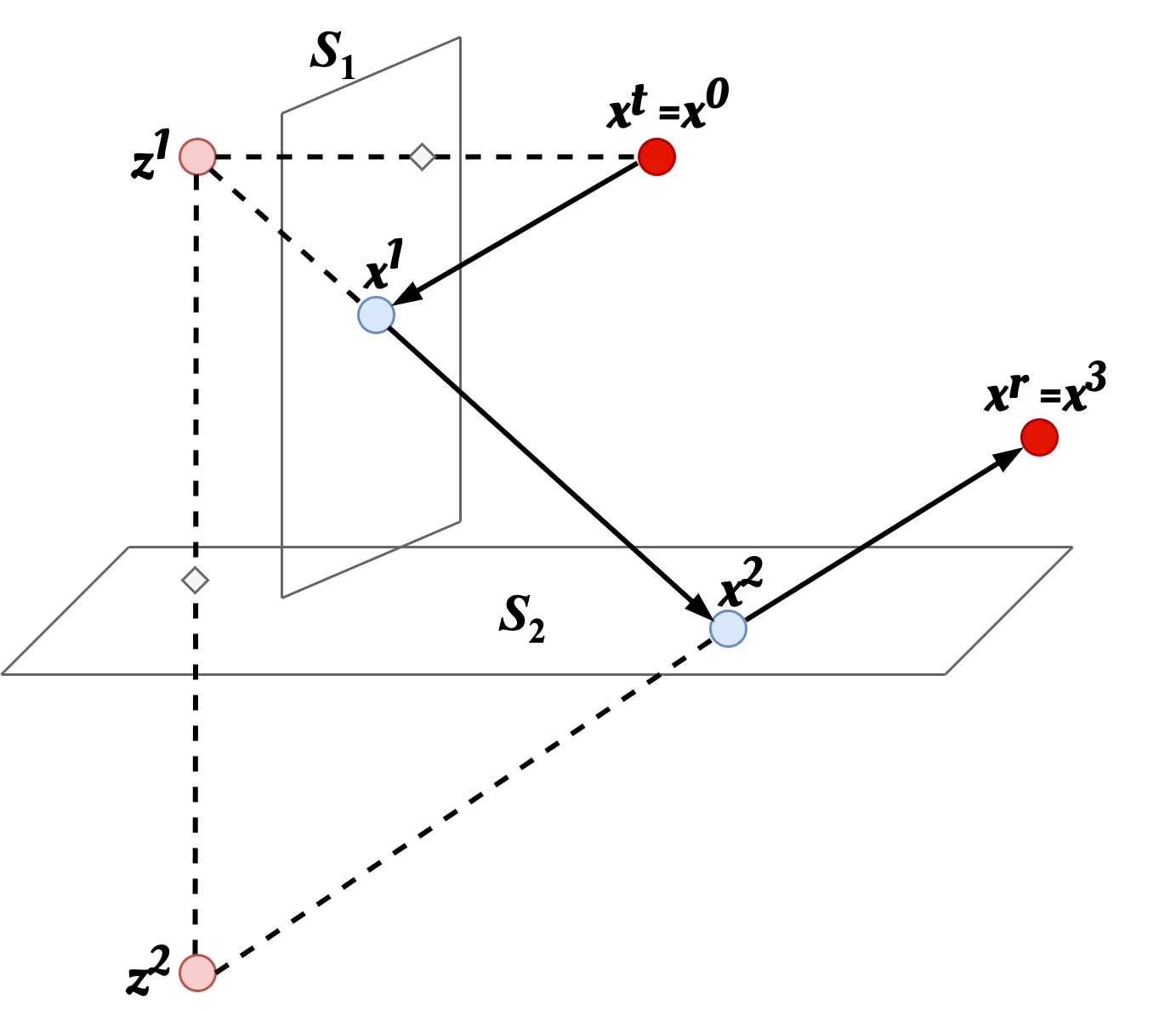
Figure 2: Example route with two reflections (i.e, $K=3$). The initial point is the transmitter, ${\boldsymbol{x}}^{t}={\boldsymbol{x}}^{0}$. The final point is the receiver, ${\boldsymbol{x}}^{r}={\boldsymbol{x}}^{K}$. The intermediate points, ${\boldsymbol{x}}^{1},{\boldsymbol{x}}^{2}$ are the locations of the reflections on the surfaces denoted $S_{1}$ and $S_{2}$.

Write the path’s route as a sequence of $K-1$ interactions:

$${\boldsymbol{x}}^{t}={\boldsymbol{x}}^{0}\rightarrow{\boldsymbol{x}}^{1}\rightarrow\cdots\rightarrow{\boldsymbol{x}}^{K}={\boldsymbol{x}}^{r},$$ (13)

where, ${\boldsymbol{x}}^{i}$ represents the location of the $i$-the reflection. The initial point, ${\boldsymbol{x}}^{0}={\boldsymbol{x}}^{t}$, is the TX location and the final point, ${\boldsymbol{x}}^{K}={\boldsymbol{x}}^{r}$, is the RX location. An example path with two reflections (i.e., $K=3$) is shown in Fig. 2. Let $S_{k}$ denote the $k$-th reflecting plane. For example, in Fig. 2, there are two surfaces, $S_{1}$ and $S_{2}$.

The key idea in the proof is to trace the reflection of the transmitted point in each surface. Simple geometry shows that, after $K$ reflections, the image of the transmitted point is an orthogonal and shifted transformation of the original point, and the path distance is the distance to this reflected point. The details are in Appendix A. ∎

We note that the distance function (12) has a simple geometric interpretation: The distance of any reflected path is identical to the distance on a LOS path but with the TX in a rotated and shifted the reference frame. The rotation is represented by the orthogonal matrix ${\boldsymbol{U}}$ and the shift by the vector ${\boldsymbol{g}}$. Returning to Fig. 1, this rotated and shifted point is simply the mirror image of the original transmitter.

It is important to recognize that, in a multi-path channel, there will be separate parameters, ${\boldsymbol{U}}_{\ell}$ and ${\boldsymbol{g}}_{\ell}$, for each path $\ell$. Thus, if we are computing a MIMO channel matrix component, $H_{mn}(f)$ in (3), each path distance function must be computed from an expression of the form:

$$d_{\ell}({\boldsymbol{x}}^{r}_{m},{\boldsymbol{x}}^{t}_{n})=\left\|{\boldsymbol{x}}^{r}_{m}-{\boldsymbol{U}}_{\ell}{\boldsymbol{x}}^{t}_{n}-{\boldsymbol{g}}_{\ell}\right\|.$$

We will discuss how to estimate the parameters $({\boldsymbol{U}}_{\ell},g_{\ell})$ for each path in Section IV.

III-B Relation to the PWA Model

The description (12) can also be easily connected to the parameters in the PWA. Let $R_{z}(\phi)$, $R_{y}(\theta)$ and $R_{x}(\gamma)$ be the rotation matrices around the $z$, $y$ and $x$ axes:

$${\boldsymbol{R}}_{z}(\phi) :=\begin{bmatrix}\cos(\phi)&-\sin(\phi)&0\\ \sin(\phi)&\cos(\phi)&0\\ 0&0&1\end{bmatrix},$$ (14a)

$${\boldsymbol{R}}_{y}(\theta) :=\begin{bmatrix}\cos(\theta)&0&\sin(\theta)\\ 0&1&0\\ -\sin(\theta)&0&\cos(\theta)\end{bmatrix}$$ (14b)

$${\boldsymbol{R}}_{x}(\gamma) :=\begin{bmatrix}1&0&0\\ 0&\cos(\gamma)&-\sin(\gamma)\\ 0&\sin(\gamma)&\cos(\gamma)\end{bmatrix}$$ (14c)

Also, for $s=\pm 1$, let ${\boldsymbol{Q}}_{z}(s)$ be the reflection in the $z$-axis:

$${\boldsymbol{Q}}_{z}(s):=\begin{bmatrix}1&0&0\\ 0&1&0\\ 0&0&s\end{bmatrix}.$$ (15)

With these definitions, we have the following result.

Theorem 2

Suppose a path has $K-1$ constant planar reflections from regions ${\mathcal{A}}^{t}$ to ${\mathcal{A}}^{r}\subset{\mathbb{R}}^{p}$. Let ${\boldsymbol{x}}^{t}_{0}\in{\mathcal{A}}^{t}$ and ${\boldsymbol{x}}^{r}_{0}\in{\mathcal{A}}^{r}$ be arbitrary points in these regions. Then, if $p=3$, there exists parameters

$$(\tau,\phi^{r},\theta^{r},\phi^{t},\theta^{t},\gamma^{t},s)$$ (16)

where

$$s=\begin{cases}-1&\mbox{if $K$ is even}\\ 1&\mbox{if $K$ is odd},\end{cases}$$ (17)

such that for all ${\boldsymbol{x}}^{r}\in{\mathcal{A}}^{r}$ and ${\boldsymbol{x}}^{t}\in{\mathcal{A}}^{t}$, the total path distance is

$$d({\boldsymbol{x}}^{r},{\boldsymbol{x}}^{t})=\Bigl{\|}c\tau{\boldsymbol{e}}_{x}+{\boldsymbol{R}}_{y}(\theta^{r}){\boldsymbol{R}}_{z}(-\phi^{r})({\boldsymbol{x}}^{r}_{0}-{\boldsymbol{x}}^{r})$$

$$+{\boldsymbol{Q}}_{z}(s){\boldsymbol{R}}_{x}(\gamma^{t}){\boldsymbol{R}}_{y}(\theta^{t}){\boldsymbol{R}}_{z}(-\phi^{t})({\boldsymbol{x}}^{t}_{0}-{\boldsymbol{x}}^{t})\Bigr{\|}.$$ (18)

Moreover the parameters $(\tau,\phi^{r},\theta^{r},\phi^{t},\theta^{t})$ match the parameters in the PWA model (II).

Proof:

See Appendices B and Appendix C. ∎

The importance of the result is that, in $p=3$, the path distance function can be explicitly written as a set of rotation angles: Specifically, there are elevation and azimuth angles, $\theta^{r}$ and $\phi^{r}$ at the RX, and roll, elevation, and azimuth angles $\gamma^{t}$, $\theta^{t}$ and $\phi^{t}$ at the TX. There is an additional binary reflection term $s$.

In a multi-path channel, there will be one set of such parameters for each path along with a path gain. Thus, if there are $L$ paths, the parameters for the channel will be

$$(g_{\ell},\tau_{\ell},\phi^{r}_{\ell},\theta^{r}_{\ell},\phi^{t}_{\ell},\theta^{t}_{\ell},\gamma^{t}_{\ell},s_{\ell}),\quad\ell=1,\ldots,L$$ (19)

where we have added the complex gain $g_{\ell}$ and delay $\tau_{\ell}$ for each path $\ell$. In comparison to the PWA model (11), there is one additional binary parameter $s_{\ell}=\pm 1$ and one additional angle $\gamma^{t}_{\ell}$ per path. We have thus found a concise parametrization of the distance function that is exact and valid for all paths with arbitrary planar reflections. We will call the parametrization (19) the reflection model (RM).

IV Fitting the RM Parameters from Ray Tracing Data

A benefit of the PWA model is that computing the terms of MIMO channel matrix (3) is computationally simple. Specifically, one typically only needs to run ray tracing once between any reference TX and RX locations ${\boldsymbol{x}}_{0}^{t}$ and ${\boldsymbol{x}}^{r}_{0}$ near the array elements. If the PWA parameters for the paths (11) can be extracted from those simulations, then for any elements close to the reference locations, the path distance and phase offset of the path can be computed from (II).

Unfortunately, this approach is not valid for wide aperture arrays where the displacements ${\boldsymbol{x}}^{t}-{\boldsymbol{x}}^{t}_{0}$ and ${\boldsymbol{x}}^{r}-{\boldsymbol{x}}^{r}_{0}$ are large. In ray tracing, the conventional approach is to perform a simulation for each pair of TX and RX elements to capture the full MIMO response accurately. Hence, if there are $N_{\rm tx}$ and $N_{\rm rx}$ elements on the TX and RX arrays, the computational complexity grows by $N_{\rm rx}N_{\rm tx}$. Moreover, if the arrays are moved or changed, the simulations need to be performed again. As ray tracing is computationally costly, performing ray tracing $N_{\rm rx}N_{\rm tx}$ times for each possible array configuration or orientation can be computationally prohibitive.

In contrast, if one has the full RM model parameters (19) for each path, the MIMO channel matrix coefficients (3) can be computed for arbitrary array geometries without re-running the ray tracing.

In this section, we show how the model parameters (19) can be extrapolated from a limited number of ray tracing simulations. We describe two potential methods:

• RM via Route Tracing (RM-RT): In this method, we assume that we can obtain the full route (13) for each path. This route is provided by most ray tracers, such as the commercial Wireless Insite ray tracer [22] that we use below. Given the route information, we show that the complete set of RM model parameters (19) can be found directly from the channel from a single pair of reference locations $({\boldsymbol{x}}^{t}_{0},{\boldsymbol{x}}^{r}_{0})$.

• RM via Displaced Pairs (RM-DP): In this case, we assume the ray tracing provides only the PWA parameters (11) for any TX-RX pair. However, the path route (13) is not provided. In this case, we show that the RM model parameters can be found from the PWA model parameters at $M+1$ TX-RX pairs with one pair being a reference pair, and $M$ additional pairs at locations displaced from the reference. The number of required additional pairs is $M\geq 2$.

IV-A Parameter Estimation via Route Tracing

In the first method, reflection model via route tracing (RM-RT), ray tracing is performed between some reference TX and RX pair locations, ${\boldsymbol{x}}_{0}^{t}$ and ${\boldsymbol{x}}_{0}^{r}$. We assume that, in addition to the PWA parameters (11), the ray tracing provides the physical route of each multi-path component. Specifically, for each path, we assume the ray tracer provides sequence of points as in (13). Under this assumption, we can obtain the parameters ${\boldsymbol{U}}$ and ${\boldsymbol{g}}$ in (12) following the proof of Theorem 1. The steps are as follows:

1. Compute the direction vector, ${\boldsymbol{v}}^{k}$, of each step from (40).

2. Compute the normal vector, ${\boldsymbol{u}}^{k}$, and intercept, $b^{k}$, to the $k$-th interacting surface from (41) and (42).

3. Compute the reflection matrix ${\boldsymbol{V}}_{k}$ and translation vector ${\boldsymbol{c}}^{k}$ in (44).

4. Compute the sequence of intercepts, ${\boldsymbol{g}}^{k}$, from (47).

5. Compute ${\boldsymbol{U}}$ and ${\boldsymbol{g}}$ from (46).

After finding ${\boldsymbol{U}}$ and ${\boldsymbol{g}}$, we can also find the parameters (19) in Theorem 2 from the proof of that theorem:

1. Compute, ${\boldsymbol{d}}_{0}$, the separation vector from the RX to the reflection TX image from (50).

2. Compute the angles $(\theta^{r}.\phi^{r})$ and distance $\tau$ by putting ${\boldsymbol{d}}_{0}$ into spherical coordinates (53).

3. Compute the binary term $s=\pm 1$ from the number of reflections, $K-1$, using (17).

4. Compute ${\boldsymbol{W}}$ from (56).

5. Since ${\boldsymbol{Q}}_{z}(s){\boldsymbol{W}}$ is an orthogonal matrix with determinant one, write the matrix as a product of rotation matrices (61) to recover the TX angles $(\gamma^{t},\theta^{t},\phi^{t})$ [23].

Again, note that this procedure is performed on each path. Hence, if the ray tracing provides $L$ paths, the procedure will be performed $L$ times, producing parameters (19) for $\ell=1,\ldots,L$.

IV-B Parameter Estimation via Displaced Pairs

In this case, we assume the ray tracer does not include full path route (13) between TX-RX pairs. Instead, the ray tracer only provides the standard PWA parameters (11) for each TX-RX pair. To obtain the RM parameters, we will perform ray tracing between a total of $M+1$ TX-RX pairs $({\boldsymbol{x}}^{t}_{m},{\boldsymbol{x}}^{r}_{m})$, $m=0,1,\ldots,M$. By convention, we will call the first pair, $({\boldsymbol{x}}^{t}_{0},{\boldsymbol{x}}^{r}_{0})$, the reference pair and the remaining $M$ pairs $({\boldsymbol{x}}^{t}_{m},{\boldsymbol{x}}^{r}_{m})$, $m=1,\ldots,M$, the displaced pairs. Between each TX-RX pair, $m=0,\ldots,M$, we assume we have PWA parameters of the form:

$$(g_{\ell m},\tau_{\ell m},\phi_{\ell m}^{r},\theta_{\ell m}^{r},\phi_{\ell m}^{t},\theta_{\ell m}^{t}),\quad\ell=1,\ldots,L_{m},$$ (20)

where $L_{m}$ is the number of paths in pair $m$, $(\phi_{\ell m}^{r},\theta_{\ell m}^{r},\phi_{\ell m}^{t},\theta_{\ell m}^{t})$ are the angles of arrival and departure of path $\ell$, $g_{\ell m}$ is its complex gain, and $\tau_{\ell m}$ is its absolute delay. We show in Appendix D that if we have this from $M\geq 2$ TX-RX displaced pairs, we can solve for all the parameters (19) in the RM model. We will call the RM parameters estimated from this procedure RM via Displaced Pairs or RM-DP.

Under the ideal assumptions of the theory – namely that all reflections are specular from surfaces with no curvature – the RM-RT and RM-DP methods will return the same parameters for the RM model. However, most ray tracers also model other interactions including diffractions, diffuse reflections, and transmissions. In addition, the curvature of surfaces may also be accounted for. In this case, RM-RT and RM-DP may return slightly different results. However, we will see in the simulations below that the differences are small.

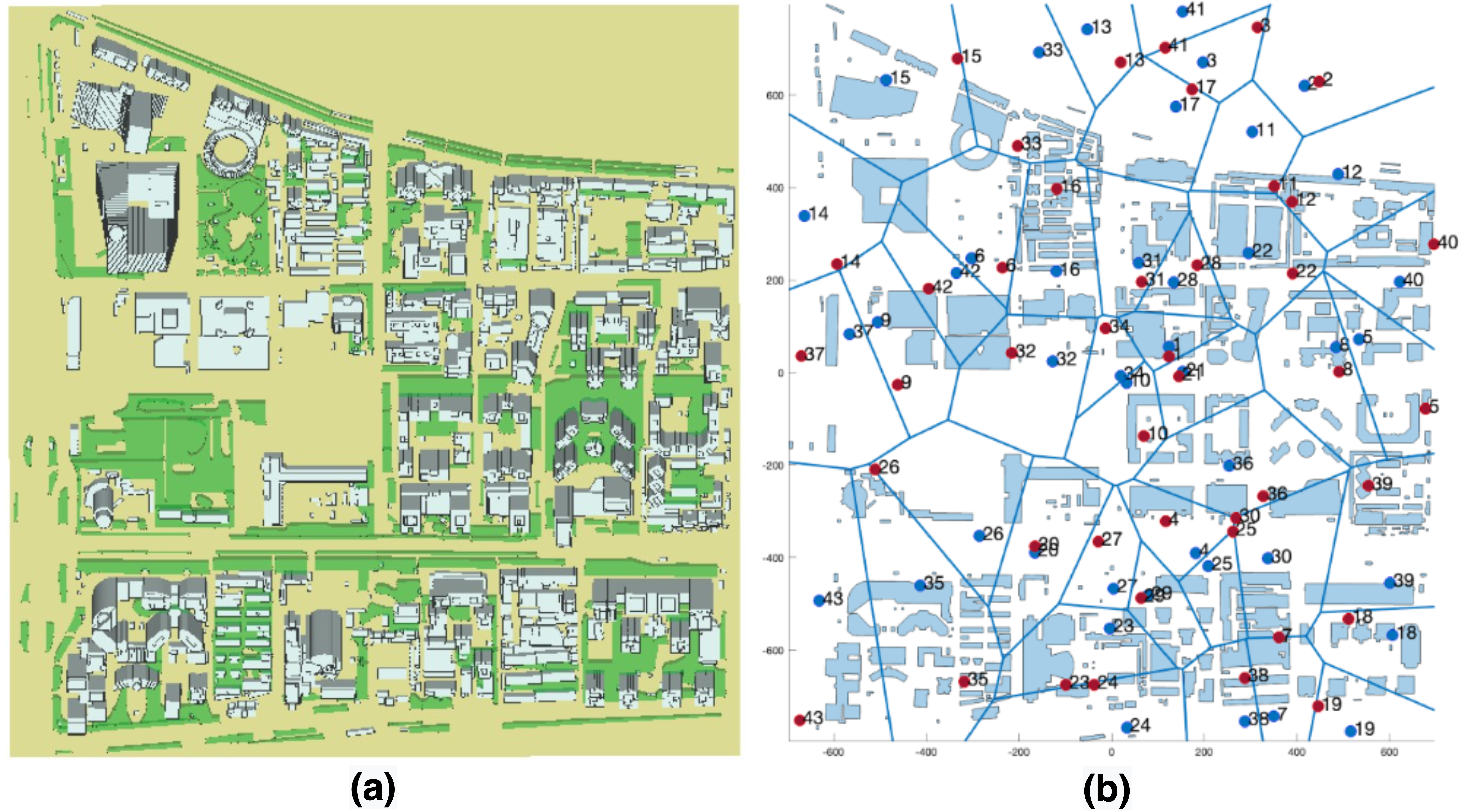
Figure 3: (a) An example of the ray tracing environment: a section of Beijing city. Foliage areas are indicated by the green blocks. (b) The distribution of reference TX and RX pairs. The transmitters and receivers are dropped randomly by implementing a Voronoi partition within our partial Beijing area.

V Validation in an Urban Environment

The RM model is exact under the ideal assumption that paths remain constant over the region of interest and that all reflections are specular and planar. Of course, in reality, these assumptions may not be exactly valid and hence the RM model may still have some errors, particularly when we are trying to estimate the channel at displacements far from the reference. To quantify this error, we conducted a ray tracing simulation of a 1650 $\times$ 1440 square meter area of a dense urban environment of Beijing, China, as shown in Fig. 3. The identical ray tracing environment was used in the channel modeling work [24]. Within this area, we selected $N=43$ TX and RX pairs spaced within $200\text{\,}\mathrm{m}$ of each other. We call each of these pairs the reference locations. For each such reference pair $({\boldsymbol{x}}^{r}_{0},{\boldsymbol{x}}^{t}_{0})$, we also generated $M=6$ random displaced locations $({\boldsymbol{x}}^{r}_{m},{\boldsymbol{x}}^{t}_{m})$, $m=1,\ldots,M$ with distances from $1\text{\,}\mathrm{c}\mathrm{m}$ to $100\text{\,}\mathrm{c}\mathrm{m}$ from the reference location. The displaced pairs are shown in Fig. 4. We then run complete ray tracing between each pair $({\boldsymbol{x}}^{r}_{m},{\boldsymbol{x}}^{t}_{m})$, $m=0,\ldots,M$, to obtain PWA parameters (20). The ray tracing is performed at two different reference RF frequencies $f_{0}=$ $28\text{\,}\mathrm{G}\mathrm{H}\mathrm{z}$ and $140\text{\,}\mathrm{G}\mathrm{H}\mathrm{z}$.

Importantly, the links in the test scenario have a significant fraction of energy where the RM model may not be exact. Table I shows the average percentage of power contributions of the ray-traced paths at the $100\text{\,}\mathrm{c}\mathrm{m}$ displacement for four categories: line of sight (LOS), reflections only, foliage, and diffraction without foliage. The RM model is theoretically exact only for the LOS and reflection paths, which constitute less than 50% of the energy for at both $28\text{\,}\mathrm{G}\mathrm{H}\mathrm{z}$ and $140\text{\,}\mathrm{G}\mathrm{H}\mathrm{z}$. Nevertheless, we will see that the RM model is able to predict the channel well.

TABLE I: Power percentage contribution

Power percentage	28 GHz-100cm	140 GHz-100cm
Paths with LoS	38.36	48.28
Paths with reflection only	4.35	4.00
Paths with foliage	57.28	47.71
Paths with diffraction and no foliage	0.01	0.01

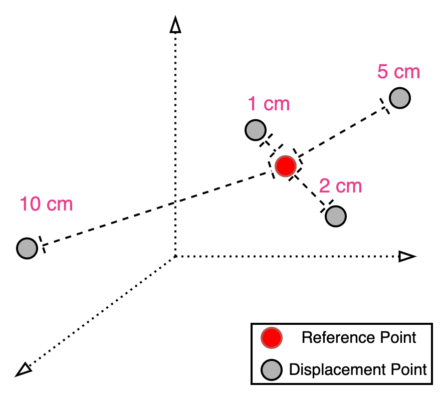
Figure 4: Random displaced pairs generation for testing: Around each location $({\boldsymbol{x}}^{r}_{0},{\boldsymbol{x}}^{t}_{0})$, we generated displaced locations at random 3D locations $({\boldsymbol{x}}^{r}_{m},{\boldsymbol{x}}^{t}_{m})$ at distances: $1\text{\,}\mathrm{c}\mathrm{m}$, $2\text{\,}\mathrm{c}\mathrm{m}$, $5\text{\,}\mathrm{c}\mathrm{m}$, $10\text{\,}\mathrm{c}\mathrm{m}$, $50\text{\,}\mathrm{c}\mathrm{m}$ and $100\text{\,}\mathrm{c}\mathrm{m}$.

Now, let $H_{m}(f)$ denote the complex channel from the ${\boldsymbol{x}}^{t}_{m}$ to ${\boldsymbol{x}}^{r}_{m}$ at an RF frequency $f$. The “true” value of this channel can be computed from the ray tracing data between the pair $({\boldsymbol{x}}^{r}_{m},{\boldsymbol{x}}^{t}_{m})$ at the reference RF frequency $f_{0}$. Specifically, the complex channel gain at any RF frequency $f$ is given by

$$H_{m}(f)=\sum_{\ell=1}^{L_{m}}g_{\ell m}e^{-j2\pi(f-f_{0})\tau_{\ell m}},$$ (21)

where $L_{m}$ is the number of paths between ${\boldsymbol{x}}^{t}_{i}$ and ${\boldsymbol{x}}^{r}_{i}$; and for path $\ell$, $g_{\ell m}$ is the complex gain of the path at the reference location and frequency, and $\tau_{\ell m}$ is its delay.

We wish to see how well different models can predict the true channels $H_{m}(f)$ between the displaced TX-RX pairs $({\boldsymbol{x}}^{r}_{m},{\boldsymbol{x}}^{t}_{m})$, using ray tracing information only near the reference TX-RX pair $({\boldsymbol{x}}^{r}_{0},{\boldsymbol{x}}^{t}_{0})$. We compare three methods:

• Constant model: $\widehat{H}_{m}(f)=H_{0}(f)$ where we assume that the channel does not change from the reference location.

• PWA model: The estimate is computed from

  $$\widehat{H}_{m}(f)=\sum_{\ell=1}^{L_{0}}g_{\ell 0}\exp\left[j2\pi\left(\tau_{\ell 0}f_{0}-\frac{f\widehat{d}_{\ell m}}{c}\right)\right],$$ (22)

  where $\widehat{d}_{\ell m}$ is the estimate of the distance $d_{\ell}({\boldsymbol{x}}^{r}_{m},{\boldsymbol{x}}^{t}_{m})$ on path $\ell$ from the PWA model (II):

  $$\widehat{d}_{\ell m}=\widehat{d}_{\ell}({\boldsymbol{x}}^{r}_{m},{\boldsymbol{x}}^{t}_{m})=c\tau_{\ell 0}$$

  $$+({\boldsymbol{u}}^{r}_{\ell 0})^{\intercal}({\boldsymbol{x}}^{r}_{0}-{\boldsymbol{x}}^{r}_{m})+({\boldsymbol{u}}^{t}_{\ell 0})^{\intercal}({\boldsymbol{x}}^{t}_{0}-{\boldsymbol{x}}^{t}_{m}),$$ (23)

  where $\tau_{\ell 0}$ is the delay between the reference pair $({\boldsymbol{x}}^{r}_{0},{\boldsymbol{x}}^{t}_{0})$ and ${\boldsymbol{u}}^{r}_{\ell 0}$ and ${\boldsymbol{r}}^{t}_{\ell 0}$ are the unit vectors in the directions of arrival and departure at the reference location:

  $${\boldsymbol{u}}^{r}_{\ell 0} =(\cos(\phi^{r}_{\ell 0})\cos(\theta^{r}_{\ell 0}),\sin(\phi^{r}_{\ell 0})\cos(\theta^{r}_{\ell 0}),\sin(\theta^{r}_{\ell 0}))$$ (24a)

  $${\boldsymbol{u}}^{t}_{\ell 0} =(\cos(\phi^{t}_{\ell 0})\cos(\theta^{t}_{\ell 0}),\sin(\phi^{t}_{\ell 0})\cos(\theta^{t}_{\ell 0}),\sin(\theta^{t}_{\ell 0})).$$ (24b)

  The channel estimate (22) thus represents the estimate based on extrapolated path distances using the PWA parameters from the reference.

• Reflection model (RM): For the reflection model, we compute the RM model parameters $({\boldsymbol{U}}_{\ell},{\boldsymbol{g}}_{\ell})$ for all paths $\ell$ using either the RM-RT or RM-DP methods in Section IV. We then use channel estimate (22) where $\widehat{d}_{\ell m}$ are the estimates of the distances $d({\boldsymbol{x}}^{r}_{m},{\boldsymbol{x}}^{t}_{m})$ computed from the reflection model (12):

  $$\widehat{d}_{\ell m}=\widehat{d}_{\ell}({\boldsymbol{x}}^{r}_{m},{\boldsymbol{x}}^{t}_{m})=\left\|{\boldsymbol{x}}^{r}_{m}-{\boldsymbol{U}}_{\ell}{\boldsymbol{x}}^{t}_{m}-{\boldsymbol{g}}_{\ell}\right\|.$$ (25)

  Equivalently, we can obtain the RM parameters (19) and use the distance (18). These two parametrizations will give the same answer.

For the reflection model, the parameters were extracted as described in Section IV by implementing both the RM-RT and RM-DP methods. In the RM-RT method, the high-precision coordinates of all interaction points between reference TX-RX pairs are exported from the ray tracer. For the RM-DP method, we used $M=2$ for the two displaced pairs at the distances $1\text{\,}\mathrm{c}\mathrm{m}$ and $2\text{\,}\mathrm{c}\mathrm{m}$ from the reference location. We used $M=2$ since, as discussed above, this value is the minimum number to uniquely identify the parameters. These are the two displaced points closest to the reference.

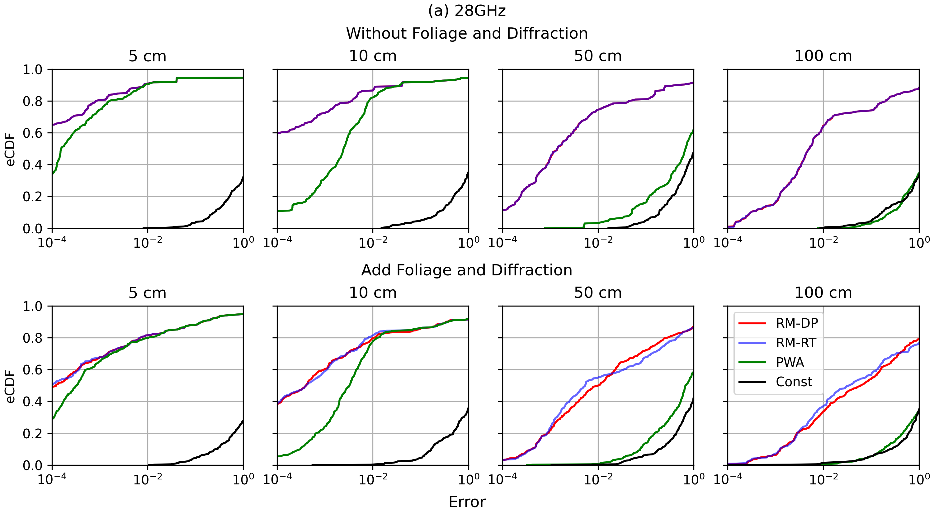
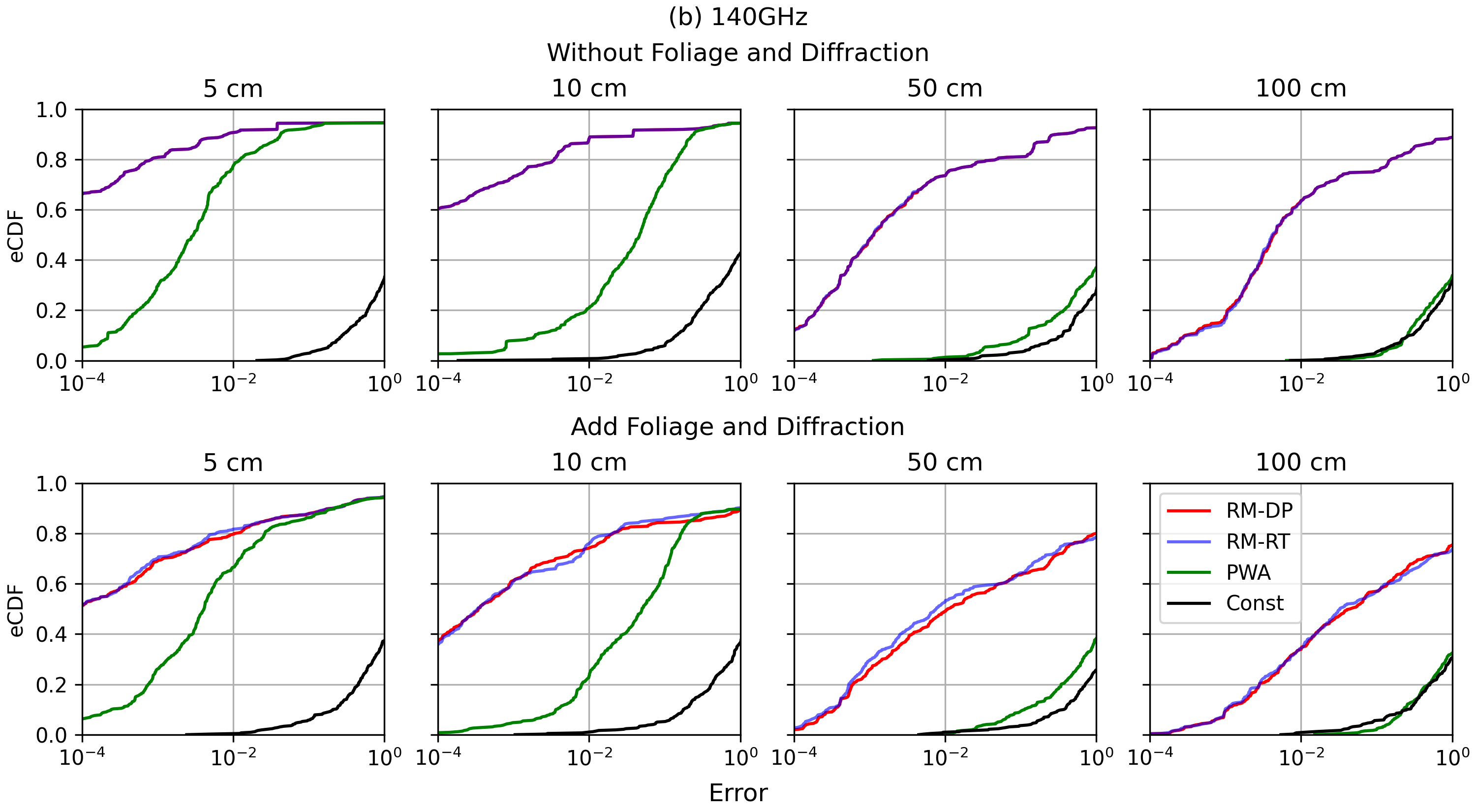
Figure 5: eCDF plot for the error of estimated channel gain in the randomized directions at different distances. The displacement distances are set to $5\text{\,}\mathrm{c}\mathrm{m}$, $10\text{\,}\mathrm{c}\mathrm{m}$, $50\text{\,}\mathrm{c}\mathrm{m}$, and $100\text{\,}\mathrm{c}\mathrm{m}$, where (a) is $28\text{\,}\mathrm{G}\mathrm{H}\mathrm{z}$; (b) is $140\text{\,}\mathrm{G}\mathrm{H}\mathrm{z}$. The RM-DP refers to the estimation of reflection model parameters via displaced pairs, while the RM-RT refers to the estimation of reflection model parameters via route tracing. And the PWA refers to the standard plane wave approximation model.

Similar to [25], we performed the validation on two bands: $28\text{\,}\mathrm{G}\mathrm{H}\mathrm{z}$ with a bandwidth of $400\text{\,}\mathrm{M}\mathrm{H}\mathrm{z}$, and $140\text{\,}\mathrm{G}\mathrm{H}\mathrm{z}$ with a bandwidth of $2\text{\,}\mathrm{G}\mathrm{H}\mathrm{z}$. On each link, the true and estimated channels were computed at the reference and displaced locations at ten random frequencies within the bandwidth. All ray tracing was performed using Wireless Insite by Remcom [22]. Importantly, the modeling also includes diffraction, so that deviations from the theory due to non-specular reflections are included. Additionally, the ray tracing can be run with or without foliage. Since interactions with foilage do not necessarily follow the theory, this feature will also enable us to measure the accuracy of the model under more realistic propagation mechanisms. The source code and data for the validation process can be found at [26].

We compute the normalized mean squared errors:

$$\epsilon_{m}(f):=\frac{\left|\widehat{H}_{m}(f)-H_{m}(f)\right|^{2}}{E_{0}},\quad E_{0}:=\sum_{\ell=1}^{L_{0}}|g_{\ell 0}|^{2}$$ (26)

which represents the channel estimate error relative to the average wideband received channel energy. This error can be interpreted as the measure of predicting the channel gain at displaced locations from ray tracing at locations close to the reference.

Fig. 5 plot the empirical cumulative distribution function of the error (26) in both $28\text{\,}\mathrm{G}\mathrm{H}\mathrm{z}$ and $140\text{\,}\mathrm{G}\mathrm{H}\mathrm{z}$. As expected, for all models, as the displacement from the reference location is increased, the error increases since we are trying to extrapolate the channel further from the reference. We also observe that the two-parameter estimation methods of the reflection model, RM-RT and RM-DP, have similar performance. This fact shows that the two-parameter estimation methods are in agreement.

Most importantly, we see that the reflection model (either RM-DP or RM-RT) obtains dramatically lower errors at high displacements than the PWA or constant model. For example, at a $100\text{\,}\mathrm{c}\mathrm{m}$ displacement, the median relative error of the RM is less than $10^{-2}$, thus enabling accurate calculation of the MIMO matrix terms with apertures of this size. In contrast, the relative error is $>1$ for the PWA and constant model. Interestingly, although the proposed reflection model is only theoretically correct for fully specular reflections, we see that low errors are obtainable even with foliage and diffraction.

VI Application for Estimation LOS/NLOS MIMO Capacity

TABLE II: Channel capacity estimation simulation parameters

Item	Value
Spectrum	Carrier frequency: 140 GHz
	Bandwidth: 2 GHz
Antenna Height	TX & RX: 2.49 m (central point)
Array Size	TX & RX: 64 (8 $\times$ 8 UPA)
Antenna Spacing	0.14 m ($\sim$65 * wavelength)
Array Aperture	0.98 m (Horizontal and Vertical)
Transmit Power	TX Array: 23 dBm
Noise Figure	3 dB
TX Array Orientation	$[-180^{\circ},180^{\circ}]$ with $15^{\circ}$ steps
RX Array Orientation	Align on boresight (face to TX)
Tx-Rx Distance	180 meters

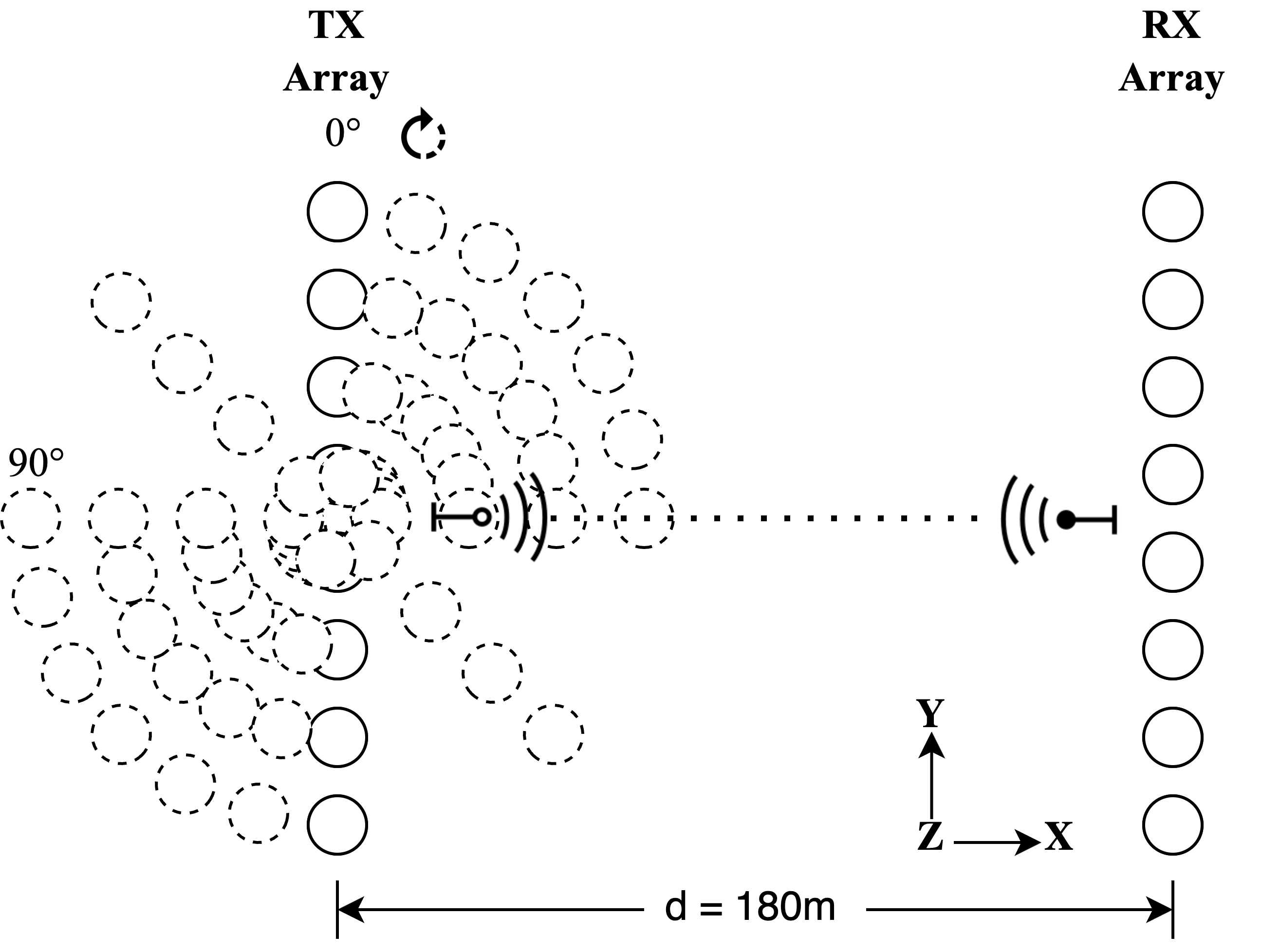
Figure 6: Illustration of TX and RX arrays orientation. The orientation of the RX array is aligned on the boresight and faces the center of the TX array. The TX array is rotated at different angles $\phi$ away from the boresight. The goal is to estimate the MIMO capacity as a function of the antenna orientation. We use values $\phi\in[-180^{\circ},180^{\circ}]$ with $15^{\circ}$ steps.

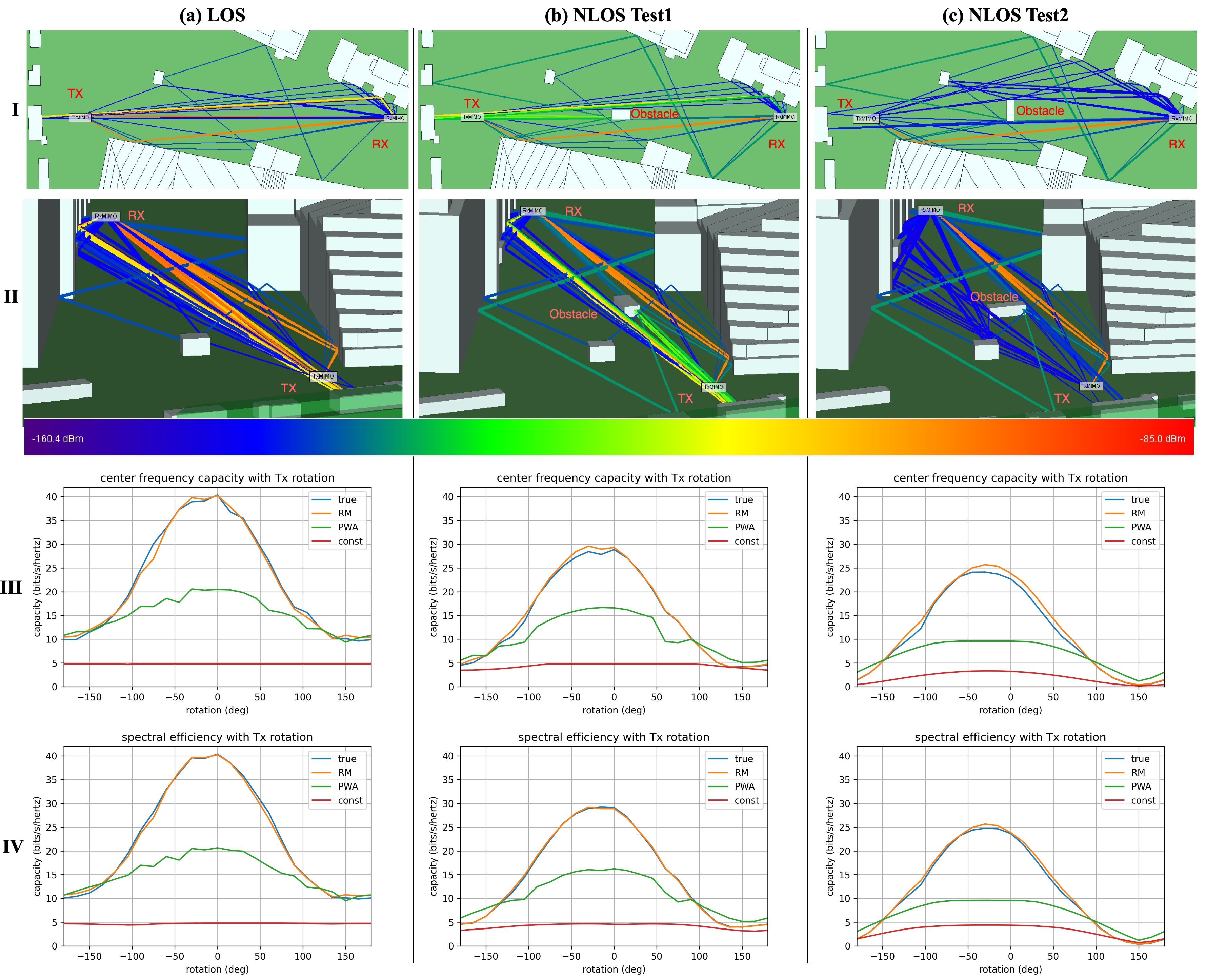
Figure 7: Channel capacity simulation results and urban test scenarios at $140\text{\,}\mathrm{G}\mathrm{H}\mathrm{z}$. There are three different test scenarios shown in Column (a, b, c). The Row I and Row II depict 2D (top-down) and 3D views of the paths between TX and RX, respectively. In each test case, the transmitter is rotated around 360^∘. Within each test case, the figures in Rows III and IV show the true and estimated capacity as a function of the TX rotation angle. Row III shows the narrowband capacity at the center frequency, and Row IV shows the average spectral efficiency across the band.

VI-A Simulation Set-Up

We conclude with a demonstration example of how the RM model can be used to significantly reduce the computation time in predicting the MIMO capacity in a wide aperture system. The parameters of the channel capacity estimation simulation are shown in the Table II.

We select a single TX and RX location pair in the Beijing area with a TX-RX separation distance of approximately $d=$ $180\text{\,}\mathrm{m}$. All simulations are performed at a carrier frequency of $f_{0}=$ $140\text{\,}\mathrm{G}\mathrm{H}\mathrm{z}$ and the bandwidth $B=$ $2\text{\,}\mathrm{G}\mathrm{H}\mathrm{z}$ – similar to what is being expected for sub-THz backhaul [10, 11, 12]. We then consider three conditions:

• Test (a): The environment with no additional obstacles. In this case, the link from the TX-RX is LOS.

• Test (b): An additional $2\times 3\times 4$ $\mathrm{m}^{3}$ obstacle (similar to a car) is placed to block the LOS path. The obstacle is oriented in the $x$-axis (east-west).

• Test (c): The identical set-up as Test (b), but the obstacle oriented in the $y$-axis (north south).

A top-down view of each of the test scenarios is shown in the middle panel of Fig. 7 and a 3D view is shown in the bottom panel. Ray tracing is run between the TX-RX locations in Tests (a)–(c) and the rays found from the ray tracing are also shown in middle and bottom panels of of Fig. 7. It can be seen that Test (a) has a LOS path while Tests (b) and (c) have only NLOS paths. All ray tracing simulations included diffraction and foliage. In particular, diffracted paths around the obstacles can be seen in Tests (b) and (c) in Fig. 7. Assuming an ideal planar reflector, the RM model would indeed be accurate. However, since actual reflectors are neither infinitely large nor perfectly planar, differences between the true and RM model arise. Nonetheless, empirical studies show that the model remains a dependable approximation even with substantial displacements.

We then place $8\times 8$ uniform planar arrays (UPAs) on both TX and RX sides with an array total aperture of $0.98\times 0.98$ $\mathrm{m}$, in which case, the antenna spacing is $0.14$ $\mathrm{m}$. We adopt the gNB antenna pattern specified by 3GPP [27].

The arrays are first aligned to each other so that their bore sights are along the LOS direction (even in Tests (b) and (c) where the LOS path is not present). We then consider azimuth rotations $\phi$ of the TX array away from bore sight. We use $N_{\rm ang}=24$ angular values of $\phi\in[-180^{\circ},180^{\circ}]$ with $15^{\circ}$ steps. The rotation is illustrated in Fig. 6.

Our goal is to estimate the MIMO capacity of this link as a function of the TX array orientation $\phi$. This type of simulation would often occur in RF planning since one may need to understand how to mount and orient the array for optimal coverage. Also, when serving multiple points, the array cannot be oriented in bore sight for all RX locations. In this case, it is valuable to be able to predict the MIMO capacity as a function of the actual orientation.

We emphasize here that our goal here is not to make a general statement on the capacity of wide aperture MIMO systems. Such an analysis would require running more extensive simulations to find the statistical distribution of the capacity over large numbers of TX-RX locations. The point of this simulation is to simply illustrate how the RM model can be used to simplify the simulation time for one such link.

VI-B Capacity Estimation via Exhaustive Ray Tracing

We first consider estimating the capacity via exhaustive ray tracing. This method is the most exact, but also the most computationally intensive. For exhaustive ray tracing, we must run ray tracing between each TX and RX element in the arrays at each orientation at some reference frequency $f_{0}$. That is, between each TX element $n$ and RX element $m$, we use ray tracing at the RF center frequency $f_{0}$ to find parameters

$$(g_{\ell mn},\tau_{\ell mn},\phi_{\ell mn}^{r},\theta_{\ell mn}^{r},\phi_{\ell mn}^{t},\theta_{\ell mn}^{t}),\quad\ell=1,\ldots,L_{mn},$$ (27)

where $L_{mn}$ is the number of paths between the TX element $n$ and RX element $n$ and the items in the vector in (27) are the gain, delays, and angles of the path $\ell$ in that link. Then, similar to the previous section, the MIMO channel matrix at a frequency $f$, can be estimated by

$${\boldsymbol{H}}(f)=\begin{bmatrix}H_{11}(f)&\dots&H_{1N_{\rm tx}}(f)\\ \vdots&\ddots&\vdots\\ H_{N_{\rm rx}1}(f)&\dots&H_{N_{\rm rx}N_{\rm tx}}(f)\end{bmatrix},$$ (28)

where

$$H_{mn}(f)=\sum_{\ell=1}^{L_{mn}}g_{\ell mn}e^{-j2\pi(f-f_{0})\tau_{\ell mn}}.$$ (29)

The capacity can then be estimated from the MIMO channel matrix from standard MIMO communication theory [15], depending on the MIMO assumptions. For example, suppose that the transmit power is $P_{\rm tx}$, the bandwidth is $B$, and the TX must transmit a constant PSD, $S_{\rm tx}=P_{\rm tx}/B$. Suppose, in addition, that the TX and RX know the MIMO channel matrix, ${\boldsymbol{H}}(f)$, at all frequencies $f$ in the band and perform optimal pre-coding at the TX and linear processing at the RX. That is, the system has full CSI-T and CSI-R. Let

$${\boldsymbol{s}}(f)=(s_{1}(f),\ldots,s_{r}(f)),$$ (30)

denote the singular values of ${\boldsymbol{H}}(f)$ at frequency $f$, where $r$ is the channel rank. Then, we can estimate the rate by

$$R:=\int_{f_{0}-B/2}^{f_{0}+B/2}\mathrm{SE}(f)\,df$$ (31)

where $\mathrm{SE}(f)$ is the spectral efficiency (i.e., rate per unit bandwidth):

$$\mathrm{SE}(f)=\max_{k=1,\ldots,r}\sum_{i=1}^{k}\rho\left(\frac{s_{i}^{2}(f)P_{\rm tx}}{N_{0}Bk}\right),$$ (32)

where $N_{0}$ is the noise PSD, $\rho(\gamma)$ is the spectral efficiency per stream for an SNR $\gamma$, and the maximization over $k$ is to select the number of streams to use. The formula (32) assumes that we allocate a fraction $1/k$ of the power to each stream and optimize over $k$. This allocation is an approximation of water-filling. The resulting average spectral efficiency is

$$\overline{\mathrm{SE}}:=R/B.$$ (33)

For the theoretical Shannon capacity, in (32), we would use the formula:

$$\rho(\gamma)=\log_{2}(1+\gamma).$$ (34)

However, to account for losses with practical codes and overhead, we assume a widely-used model in 3GPP simulations [28]:

$$\rho(\gamma):=\min\left\{\alpha\log_{2}(1+\gamma),\rho_{\rm max}\right\}$$ (35)

where $\alpha=0.6$ and $\rho_{\rm max}=4.8$ $\mathrm{b}\mathrm{p}\mathrm{s}\mathrm{/}\mathrm{H}\mathrm{z}$.

The key computational challenge in the exhaustive capacity estimation is the ray tracing. Since the arrays have $N_{\rm rx}=N_{\rm tx}=64$ elements each, and there are $N_{\rm ang}=24$ angular steps, we must run ray tracing $N$ times with

$$N=N_{\rm rx}N_{\rm tx}N_{\rm ang}=(64)(64)(24)\approx 98000,$$ (36)

to extract the parameters (27) for all the angular steps. While the exhaustive procedure is the most accurate, the large number of ray tracing simulations required can be computationally extremely expensive.

To illustrate the possible gains, Table III shows the computation time of each of the main steps for the exhaustive procedure and the RM-DP and RM-RT methods. All times are on a machine with NVIDIA RTX 3090 and Intel i9-10900K. The exhaustive method requires significantly more time due to the need to perform ray tracing at each of the $N_{\rm ang}=24$ angular rotations and for all the TX-RX pairs. In contrast, the RM-DP and RM-RT methods require ray tracing only once or twice. The RM-DP and RM-DT methods require a parameter extraction component that is not needed for the exhaustive method – but this step is negligible in computation time. All methods require similar time to compute the channels from the rays, but again, this step is also small. Overall, RM-DP and RM-RT are 150 to 200 times faster than the exhaustive method.

Table III also shows the computational time for the standard PWA method. We see that the proposed RM-DP and RM-RT are slightly longer due to the computation of the distance with the orthogonal matrix. However, the total computational time for RM-RT and RM-DP is approximately only 30 to 60% more than PWA and, as we will see, offers a much more accurate channel estimate.

Of course, the absolute numbers will depend on the machine used. However, given the massive reduction in ray tracing needed, the general trend will likely hold across platforms.

TABLE III: Computational time comparison.

	Exhaustive	PWA	RM-DP	RM-RT
Ray Tracing (min)	$65.4$ $\times 24$	2.1	4.3	2.1
Parameter Estimation (sec)	-	-	0.0014	0.0023
Channel Computation (sec)	$7.31$ $\times 24$	$9.59$ $\times 24$	$14.57$ $\times 24$	$15.11$ $\times 24$
Total (min)	1572.5	5.9	10.1	8.1

Note that the purpose here is not to suggest a particular MIMO scheme. For example, in certain scenarios, CSI-T may not be available. In these cases, the rate formula may be different. However, whatever the scheme is used, one will similarly need to compute the channel matrix at different array configurations, and the same computational complexity problem will hold. We simply select the above MIMO capacity problem since these computational difficulties are clear to see.

VI-C Approximate Capacity Estimation

Similar to Section V, we next consider the approximate capacity estimation using constant, PWA, or RM channel estimates. While these methods are approximate, the advantage is that, instead of running $N$ ray tracing simulations, where $N$ is given in (36), we only need to run a single ray tracing simulation between a reference location ${\boldsymbol{x}}^{t}_{0}$ in the center of the TX array and a reference location ${\boldsymbol{x}}^{r}_{0}$ in the center of the RX array. The MIMO channel, with any array orientation, can be then estimated from this ray tracing data, providing a much more computationally efficient approach to estimating the capacity. Our interest is in comparing the quality of this capacity estimate for different methods.

The details of the process are as follows: The ray tracing provides the PWA parameters (11) between the reference TX-RX pair $({\boldsymbol{x}}^{t}_{0},{\boldsymbol{x}}^{r}_{0})$. Similar to Section V, we consider three possible approximations for the MIMO channel matrices $H_{mn}(f)$: A constant, PWA, and RM model. Each model provides an estimate for the channel, $\widehat{H}_{mn}(f)$. The formula for these estimates is similar to Section V. For example, the PWA and RM model provide estimates $\widehat{d}_{\ell mn}$ of the delay from TX element $n$ to RX element $m$ on path $\ell$. The delay estimates can then be used in a formula similar to (22) to estimate $\widehat{H}_{mn}(f)$. The channel estimates $\widehat{H}_{mn}$ can then be used in place of the true coefficients $H_{mn}(f)$ in (29). Then, the achievable rate $R$ in (31) can be estimated using the channel estimates to obtain an approximation of $R$.

VI-D Results

The third and fourth rows of Fig. 7 show the MIMO channel center frequency capacity and spectral efficiency, $R/B$, as a function of the angle $\phi$, where the true channel, computed from exhaustive ray tracing, is used. And we simplify the integral in (31) for computing $R$ by summation over ten uniformly distributed frequencies within the bandwidth. As expected, the true channel capacity of the LOS link is greater than that of NLOS links. Also, the LOS capacity is maximized by when the arrays are pointed at bore sight. For the NLOS cases, the optimal pointing angle is slightly off bore sight to capture dominant reflections.

Also plotted in the fourth row of Fig. 7 is the capacity estimate using different channel estimates for different methods. We see that the capacity estimate by the RM model is close to the true capacity. Indeed, the overall error of the RM’s estimation of channel capacity is less than $5\%$. In contrast, the PWA and constant model grossly under-predict the capacity.

Overall, we see that the RM model can provide an estimate of the capacity of a wide aperture array $140\text{\,}\mathrm{G}\mathrm{H}\mathrm{z}$ system in a complex urban environment with reflections. Specifically, the RM model matches the capacity estimated via exhaustive ray tracing, but comes with a dramatically lower simulation time. While exhaustive ray tracing requires one ray tracing simulation between every TX-RX element and every array configuration, RM requires a single ray tracing simulation. The PWA and constant models also save the ray tracing, but are grossly inaccurate for wide aperture arrays.

VII Conclusions

Near-field communication is a promising technology for systems in the mmWave and THz bands. However, accurate assessment of near-field communications requires channel models that can capture the spherical nature of the wavefront of each path, a feature not accounted for in most models today that use planar approximations of waves. This paper has presented a simple parametrization for multi-path wireless channels that correctly describes the spherical nature of each wavefront. Interestingly, the parametrization requires only two additional parameters relative to standard plane wave models. Moreover, we have provided a computationally simple algorithm to extract the parameters from ray tracing.

The model is based on image theory and is fully accurate under the assumption of planar, infinite surface reflections. Moreover, our simulations show that the proposed reflection model delivers a high accuracy over wide apertures, even when these exact conditions are not met. In particular, the models are significantly more accurate than models based on plane wave approximations. The technique is precise while substantially decreasing the simulation duration in contrast to the comprehensive ray tracing approach.

Going forward, the method can greatly enhance the evaluation of near-field communications in site-specific settings. In this paper, we have demonstrated the method for evaluation of mmWave and sub-THz wide-aperture MIMO backhaul links in a site-specific setting.

A natural next step is to develop statistical channel models, such as those used by 3GPP [14], or machine learning methods [24, 29], that describe the distribution of these parameters in common environments.

Appendix A Proof of Theorem 1

Write the path’s route as a sequence of $K-1$ interactions as in (13). Let $S_{k}$ denote the $k$-th reflecting plane. The initial transmitter point ${\boldsymbol{x}}^{t}$ can be reflected across the surface $S_{1}$ to obtain an image that we will denote ${\boldsymbol{z}}^{1}$. This image point can in turn be reflected to create a second image ${\boldsymbol{z}}^{2}$. After $K-1$ reflections, we obtain a final image point ${\boldsymbol{z}}^{K-1}$.

The method of images states that the total distance of the reflected path is equal to the LOS distance from the final reflected image point ${\boldsymbol{z}}^{K-1}$ to the receiver ${\boldsymbol{x}}^{r}$. Hence,

$$d({\boldsymbol{x}}^{r},{\boldsymbol{x}}^{t})=\|{\boldsymbol{x}}^{r}-{\boldsymbol{z}}^{K-1}\|.$$ (37)

Therefore, (12) will be proven if we can show

$${\boldsymbol{z}}^{K-1}={\boldsymbol{U}}{\boldsymbol{x}}^{t}+{\boldsymbol{g}},$$ (38)

for some orthogonal matrix ${\boldsymbol{U}}$ and vector ${\boldsymbol{g}}$. That is, the image point is a rotation and translation of the original transmitted point.

Finding the matrix ${\boldsymbol{U}}$ and vector ${\boldsymbol{g}}$ in (38) is a matter of simple geometry. We will walk through the details since this process will also show how to numerically compute the parameters from the route sequence (13).

First, since each surface is a plane, the surface can be represented as:

$$S_{k}=\left\{{\boldsymbol{x}}~{}|~{}({\boldsymbol{u}}^{k})^{\intercal}{\boldsymbol{x}}=b^{k}\right\},$$ (39)

for some unit vector ${\boldsymbol{u}}^{k}$ and constant $b^{k}$. To compute the normal vector, let ${\boldsymbol{v}}^{k}$ be the unit vector of the $k$-th step in the route:

$${\boldsymbol{v}}^{k}=\frac{{\boldsymbol{x}}^{k}-{\boldsymbol{x}}^{k-1}}{\|{\boldsymbol{x}}^{k}-{\boldsymbol{x}}^{k-1}\|},\quad k=1,\ldots,K.$$ (40)

Then, the normal vector for $S_{k}$ is given by:

$${\boldsymbol{u}}^{k}:=\frac{{\boldsymbol{v}}^{k+1}-{\boldsymbol{v}}^{k}}{\|{\boldsymbol{v}}^{k+1}-{\boldsymbol{v}}^{k}\|},\quad k=1,\ldots,K-1.$$ (41)

Also, since we know ${\boldsymbol{x}}^{k}$ is in the plane $S_{k}$ in (39), the intercept must be given by:

$$b^{k}=({\boldsymbol{u}}^{k})^{\intercal}{\boldsymbol{x}}^{k}.$$ (42)

Since the image point ${\boldsymbol{z}}^{k}$ is the reflection of ${\boldsymbol{z}}^{k-1}$ around $S_{k}$, the two points are related by:

$${\boldsymbol{z}}^{k} ={\boldsymbol{x}}^{k-1}-2{\boldsymbol{u}}^{k}(({\boldsymbol{u}}^{k})^{\intercal}{\boldsymbol{z}}^{k-1}-b^{k})$$

$$={\boldsymbol{V}}_{k}{\boldsymbol{z}}^{k-1}+{\boldsymbol{c}}_{k}$$ (43)

where

$${\boldsymbol{V}}_{k}={\boldsymbol{I}}-2{\boldsymbol{u}}^{k}({\boldsymbol{u}}^{k})^{\intercal},\quad{\boldsymbol{c}}_{k}=2b^{k}{\boldsymbol{u}}^{k}.$$ (44)

The recursion (43) should be initialized with ${\boldsymbol{z}}^{0}={\boldsymbol{x}}^{t}$. Solving (43), we obtain

$${\boldsymbol{z}}^{k}={\boldsymbol{U}}_{k}{\boldsymbol{x}}^{t}+{\boldsymbol{g}}^{k},$$ (45)

where

$${\boldsymbol{U}}_{k}=\prod_{i=1}^{k}{\boldsymbol{V}}_{i},$$ (46)

and ${\boldsymbol{g}}^{k}$ satisfies the recursions

$${\boldsymbol{g}}^{k}={\boldsymbol{c}}^{k}+{\boldsymbol{V}}_{k}{\boldsymbol{g}}^{k-1},\quad k=1,\ldots,K-1,$$ (47)

with the initial condition ${\boldsymbol{g}}^{0}=0$. Iterating through (43), we obtain that the final image point is given by (38) with

$${\boldsymbol{U}}=\prod_{k=1}^{K-1}{\boldsymbol{V}}_{k},\quad{\boldsymbol{g}}={\boldsymbol{g}}^{K-1}.$$ (48)

Also, each matrix ${\boldsymbol{V}}_{k}$ in (44) is orthogonal. In fact, it is a Housholder matrix. Since ${\boldsymbol{U}}$ in (46) is the product of these matrices, ${\boldsymbol{U}}$ is also orthogonal. This completes the proof.

Appendix B Proof of Theorem 2

From Theorem 1, we know the distance function $d({\boldsymbol{x}}^{r},{\boldsymbol{x}}^{t})$ can be written as (12) for some matrix ${\boldsymbol{U}}$ and translation vector ${\boldsymbol{g}}$. So, we can prove the theorem if we can rewrite (12) as (18). Let ${\boldsymbol{z}}_{0}^{t}$ denote the reflected image of the TX reference ${\boldsymbol{x}}^{t}_{0}$:

$${\boldsymbol{z}}_{0}^{t}:={\boldsymbol{U}}{\boldsymbol{x}}^{t}_{0}+{\boldsymbol{g}},$$ (49)

and let ${\boldsymbol{d}}_{0}$ denote the vector from the RX to the reflection of the TX:

$${\boldsymbol{d}}_{0}:={\boldsymbol{x}}^{r}_{0}-{\boldsymbol{z}}^{t}_{0}={\boldsymbol{x}}^{r}_{0}-{\boldsymbol{U}}{\boldsymbol{x}}^{t}_{0}-{\boldsymbol{g}}.$$ (50)

Then, for any points ${\boldsymbol{x}}^{t}$ and ${\boldsymbol{x}}^{r}$, we can subtract off ${\boldsymbol{x}}^{t}_{0}$ and ${\boldsymbol{x}}^{r}_{0}$ to rewrite (12) as

$$d({\boldsymbol{x}}^{r},{\boldsymbol{x}}^{t})=\Bigl{\|}{\boldsymbol{x}}^{r}-{\boldsymbol{x}}^{r}_{0}-{\boldsymbol{U}}({\boldsymbol{x}}^{t}-{\boldsymbol{x}}^{t}_{0})+{\boldsymbol{d}}_{0}\Bigr{\|},$$ (51)

Next, let

$$\tau=\frac{1}{c}\|{\boldsymbol{d}}_{0}\|,$$ (52)

which represents the time of flight from the reference RX to the reflected image of the TX. Since ${\boldsymbol{d}}_{0}\in{\mathbb{R}}^{3}$ with $\|{\boldsymbol{d}}_{0}\|=c\tau$, we can write ${\boldsymbol{d}}_{0}$ in spherical coordinates:

$${\boldsymbol{d}}_{0}=c\tau(\cos\theta^{r}\cos\phi^{r},\cos\theta^{r}\sin\phi^{r},-\sin\theta^{r}).$$ (53)

for angles $\phi^{r}$ and $\theta^{r}$. The spherical coordinates (53) can also be written as:

$${\boldsymbol{R}}_{y}(\theta^{r}){\boldsymbol{R}}_{z}(-\phi^{r}){\boldsymbol{d}}_{0}=c\tau{\boldsymbol{e}}_{x},$$ (54)

where ${\boldsymbol{e}}_{x}=(1,0,0)$ is the unit vector in the $x$-direction. Substituting (54) into (51), we obtain

$$d({\boldsymbol{x}}^{r},{\boldsymbol{x}}^{t})\stackrel{{\scriptstyle(a)}}{{=}}\Bigl{\|}{\boldsymbol{R}}_{y}(\theta^{r}){\boldsymbol{R}}_{z}(-\phi^{r})$$

$$\qquad\times\left[({\boldsymbol{x}}^{r}-{\boldsymbol{x}}^{r}_{0})-{\boldsymbol{U}}({\boldsymbol{x}}^{t}-{\boldsymbol{x}}^{t}_{0})+{\boldsymbol{d}}_{0}\right]\Bigr{\|}$$

$$\stackrel{{\scriptstyle(b)}}{{=}}\Bigl{\|}{\boldsymbol{R}}_{y}(\theta^{r}){\boldsymbol{R}}_{z}(-\phi^{r})({\boldsymbol{x}}^{r}-{\boldsymbol{x}}^{r}_{0})$$

$$\qquad+{\boldsymbol{W}}({\boldsymbol{x}}^{t}-{\boldsymbol{x}}^{t}_{0})+c\tau{\boldsymbol{e}}_{x}\Bigr{\|},$$ (55)

where the first step (a) follows from (51) and the fact that ${\boldsymbol{R}}_{y}(\theta^{r}){\boldsymbol{R}}_{z}(-\phi^{r})$ is a rotation matrix that does not change distance, and, in step (b), we define

$${\boldsymbol{W}}:=-{\boldsymbol{R}}_{y}(\theta^{r}){\boldsymbol{R}}_{z}(-\phi^{r}){\boldsymbol{U}}.$$ (56)

Also, each Householder matrix ${\boldsymbol{V}}_{k}$ in (44) is orthogonal with determinant, $\mathrm{det}({\boldsymbol{V}}_{k})=-1$. Hence, the determinant ${\boldsymbol{U}}$ in (46) is:

$$\mathrm{det}({\boldsymbol{U}})=(-1)^{K-1}.$$ (57)

Taking the determinant of the product (56),

$$\mathrm{det}({\boldsymbol{W}}) =\mathrm{det}\left[-{\boldsymbol{R}}_{y}(\theta^{r}){\boldsymbol{R}}_{z}(-\phi^{r}){\boldsymbol{U}}\right]$$

$$=(-1)^{2}\mathrm{det}\left[{\boldsymbol{R}}_{y}(\theta^{r}){\boldsymbol{R}}_{z}(-\phi^{r})\right]\mathrm{det}({\boldsymbol{U}})$$

$$=(-1)^{K+3}=s,$$ (58)

where $s=\pm 1$ as defined in (17), and we have used the fact that the determinant of rotation matrices is one. Multiplying by the matrix ${\boldsymbol{Q}}_{z}(s)$ defined in (15), we obtain

$$\mathrm{det}\left[{\boldsymbol{Q}}_{z}(s){\boldsymbol{W}}\right]=\mathrm{det}({\boldsymbol{Q}}_{z}(s))\mathrm{det}({\boldsymbol{W}})=s^{2}=1.$$ (59)

Hence ${\boldsymbol{Q}}_{z}(s){\boldsymbol{W}}$ is an orthogonal matrix with determinant of one in ${\mathbb{R}}^{3\times 3}$. That is, the matrix is in the special orthogonal group of rotations $SO(3)$. Any such matrix can be parameterized by three rotations:

$${\boldsymbol{Q}}_{z}(s){\boldsymbol{W}}={\boldsymbol{R}}_{x}(\gamma^{t}){\boldsymbol{R}}_{y}(\theta^{t}){\boldsymbol{R}}_{z}(-\phi^{t}).$$ (60)

Since ${\boldsymbol{Q}}_{z}(s)^{2}={\boldsymbol{I}}$,

$${\boldsymbol{W}}={\boldsymbol{Q}}_{z}(s){\boldsymbol{R}}_{x}(\gamma^{t}){\boldsymbol{R}}_{y}(\theta^{t}){\boldsymbol{R}}_{z}(-\phi^{t}).$$ (61)

Substituting (61) into (55) proves (18).

It remains to show that parameters $(\theta^{r},\phi^{r},\theta^{t},\phi^{t})$ match those in the PWA model. This equivalency is shown in Appendix C.

Appendix C Equivalency of the RM and PWA Parameters

Let

$$(\theta^{r},\phi^{r},\theta^{t},\phi^{t})$$ (62)

be the angles for the RM model derived in the Appendix B. We need to show that these angles are identical to the angles in the PWA model. To this end, let ${\boldsymbol{u}}^{r}$ and ${\boldsymbol{u}}^{t}$ be the direction vectors (10), computed from these RM angles (62):

$${\boldsymbol{u}}^{r} =(\cos(\phi^{r})\cos(\theta^{r}),\sin(\phi^{r})\cos(\theta^{r}),\sin(\theta^{r}))$$ (63a)

$${\boldsymbol{u}}^{t} =(\cos(\phi^{t})\cos(\theta^{t}),\sin(\phi^{t})\cos(\theta^{t}),\sin(\theta^{t})),$$ (63b)

where, similar to Appendix B, we have dropped the dependence on $\ell$ to simplify the notation. We will show that the direction vectors (63) satisfy the directional derivative property (8):

$$({\boldsymbol{u}}^{r})^{\intercal}=-\frac{\partial d_{\ell}({\boldsymbol{x}}^{r}_{0},{\boldsymbol{r}}^{t}_{0})}{\partial{\boldsymbol{x}}^{r}},\quad({\boldsymbol{u}}^{r})^{\intercal}=-\frac{\partial d_{\ell}({\boldsymbol{x}}^{r}_{0},{\boldsymbol{r}}^{t}_{0})}{\partial{\boldsymbol{x}}^{t}}.$$

$$({\boldsymbol{u}}^{r})^{\intercal}=-\frac{\partial d_{\ell}({\boldsymbol{x}}^{r}_{0},{\boldsymbol{x}}^{t}_{0})}{\partial{\boldsymbol{x}}^{r}},\quad({\boldsymbol{u}}^{r})^{\intercal}=-\frac{\partial d_{\ell}({\boldsymbol{x}}^{r}_{0},{\boldsymbol{x}}^{t}_{0})}{\partial{\boldsymbol{x}}^{t}}.$$ (64)

Hence the directions (63) must match the PWA directions, and therefore, so must the angles.

To prove (64), write the distance in (18) as:

$$d({\boldsymbol{x}}^{r},{\boldsymbol{x}}^{t})=f({\boldsymbol{z}}),$$ (65)

where

$$f({\boldsymbol{z}}):=\|c\tau{\boldsymbol{e}}_{x}+{\boldsymbol{z}}\|,$$ (66)

and

$${\boldsymbol{z}}={\boldsymbol{R}}_{y}(\theta^{r}){\boldsymbol{R}}_{z}(-\phi^{r})({\boldsymbol{x}}^{r}_{0}-{\boldsymbol{x}}^{r})$$

$$+{\boldsymbol{Q}}_{z}(s){\boldsymbol{R}}_{x}(\gamma^{t}){\boldsymbol{R}}_{y}(\theta^{t}){\boldsymbol{R}}_{z}(-\phi^{t})({\boldsymbol{x}}^{t}_{0}-{\boldsymbol{x}}^{t}).$$ (67)

Then,

$$\frac{\partial d_{\ell}({\boldsymbol{x}}^{r}_{0},{\boldsymbol{x}}^{t}_{0})}{\partial{\boldsymbol{x}}^{r}}\stackrel{{\scriptstyle(a)}}{{=}}\left.\frac{\partial f({\boldsymbol{z}})}{\partial{\boldsymbol{z}}}\right|_{{\boldsymbol{z}}=\boldsymbol{0}}\left.\frac{\partial{\boldsymbol{z}}}{\partial{\boldsymbol{x}}^{r}}\right|_{{\boldsymbol{x}}^{r}={\boldsymbol{x}}^{r}_{0}}$$

$$\stackrel{{\scriptstyle(b)}}{{=}}{\boldsymbol{e}}_{x}^{\intercal}\left.\frac{\partial{\boldsymbol{z}}}{\partial{\boldsymbol{x}}^{r}}\right|_{{\boldsymbol{x}}^{r}={\boldsymbol{x}}^{r}_{0}}$$

$$\stackrel{{\scriptstyle(c)}}{{=}}-{\boldsymbol{e}}_{x}^{\intercal}{\boldsymbol{R}}_{y}(\theta^{r}){\boldsymbol{R}}_{z}(-\phi^{r})\stackrel{{\scriptstyle(d)}}{{=}}-({\boldsymbol{u}}^{r})^{\intercal},$$ (68)

where (a) follows from (65) and chain rule; (b) follows from taking the derivative of $f({\boldsymbol{z}})$ in (66); (c) follows from taking the derivative of ${\boldsymbol{z}}$ in (C); and (d) follows from applying the formulae for the rotation matrices in (14) and the definition of ${\boldsymbol{u}}^{r}$ in (63). Thus, (68) proves the first equation in (64). The derivative with respect to ${\boldsymbol{x}}^{t}$ is proven similarly.

Appendix D Estimation via Displaced Pairs

The details of the RM-DP fitting procedure are as follows: We assume we have PWA parameters (20) between $M+1$ TX-RX pairs, $({\boldsymbol{x}}^{t}_{m},{\boldsymbol{x}}^{r}_{m})$, $m=0,\ldots,M$. As mentioned in Section IV-B, the pair $({\boldsymbol{x}}^{t}_{0},{\boldsymbol{x}}^{r}_{0})$ is the reference pair and $({\boldsymbol{x}}^{t}_{0},{\boldsymbol{x}}^{r}_{0})$, $m=1,\ldots,M$, are the $M$ displaced pairs. The goal is to determine the RM parameters (19) at the reference pair $({\boldsymbol{x}}^{t}_{0},{\boldsymbol{x}}^{r}_{0})$. We can obtain most of the RM model parameters from the PWA parameters at the reference pair $({\boldsymbol{x}}^{t}_{0},{\boldsymbol{x}}^{r}_{0})$. Specifically, we set the number of paths at the reference pair to $L=L_{0}$, and for each path $\ell$, we set:

$$g_{\ell} =g_{\ell 0},\quad\tau_{\ell}=\tau_{\ell 0},$$ (69a)

$$\phi_{\ell}^{r} =\phi_{\ell 0}^{r},\quad\theta_{\ell}^{r}=\theta_{\ell 0}^{r},$$ (69b)

$$\phi_{\ell}^{t} =\phi_{\ell 0}^{t},\quad\theta_{\ell}^{t}=\theta_{\ell 0}^{t},$$ (69c)

The only parameters in the RM model that need to be determined are the binary variable $s_{\ell}$ and angle $\gamma_{\ell}$. each path $\ell$.

We proceed in two phases: Path matching and angle solving.

Path matching

If the displaced locations are close to the reference location, the number of paths should be the same, and the paths should approximately agree except for the change in the path distance. However, the ray tracing generally outputs paths in an arbitrary order. So, we first perform a heuristic path matching as follows. Let

$$D_{m}(\ell,\ell^{\prime}):=c_{0}\left[|\phi_{\ell 0}^{r}-\phi_{\ell^{\prime}m}^{r}|+|\phi_{\ell 0}^{t}-\phi_{\ell^{\prime}m}^{t}|\right]$$

$$+c_{1}\left[|\theta_{\ell 0}^{r}-\theta_{\ell^{\prime}m}^{r}|+|\theta_{\ell 0}^{t}-\theta_{\ell^{\prime}m}^{t}|\right],$$ (70)

which represents a distance between the parameters for the path $\ell$ in the reference pair and the path $\ell^{\prime}$ in the displaced pair $m$. The coefficients $c_{i}$ are weighting parameters that we take as

$$c_{0}=c_{1}=\frac{1}{180^{\circ}},\quad$$

To match the paths, we then perform the following recursion:

$$\sigma_{m}(\ell) =\operatorname{arg~{}min}_{\ell^{\prime}\not\in I_{\ell}}D_{m}(\ell,\ell^{\prime}),$$ (71a)

$$I_{m,\ell+1} =I_{m,\ell}\cup\sigma_{m}(\ell).$$ (71b)

which is initialized with $I_{m,0}=\varnothing$. For each path $\ell$ between the reference TX-RX pair $({\boldsymbol{x}}^{t}_{0},{\boldsymbol{x}}^{r}_{0})$, the recursion (71) finds a closest path $\ell^{\prime}=\sigma_{m}(\ell)$ in the displaced pair $({\boldsymbol{x}}^{t}_{m},{\boldsymbol{x}}^{r}_{m})$. The recursion is performed from the strongest path to the weakest path, meaning they are sorted in descending order of $|g_{\ell 0}|$. This sorting ensures that the the strongest paths are given the highest priority in the matching.

After the path matching, we reorder the paths in all the displaced pairs so that in the new order path $\ell$ in reference pair $m$ corresponds to the previous path index $\sigma_{m}(\ell)$.

Angle Solving

After the path matching is performed we can solve for the binary variable $s_{\ell}$ and angle $\gamma_{\ell}$ for each path as follows. Using the RM parameters at the reference location $m=0$, the distance along path $\ell$ between any TX-RX pair $({\boldsymbol{x}}^{t},{\boldsymbol{x}}^{r})$ is:

$$d_{\ell}({\boldsymbol{x}}^{r},{\boldsymbol{x}}^{t})=\Bigl{\|}c\tau_{\ell 0}{\boldsymbol{e}}_{x}+{\boldsymbol{R}}_{y}(\theta^{r}_{\ell 0}){\boldsymbol{R}}_{z}(-\phi^{r}_{\ell 0})({\boldsymbol{x}}^{r}_{0}-{\boldsymbol{x}}^{r})$$

$$+{\boldsymbol{Q}}_{z}(s_{\ell 0}){\boldsymbol{R}}_{x}(\gamma^{t}_{\ell 0}){\boldsymbol{R}}_{y}(\theta^{t}_{\ell 0}){\boldsymbol{R}}_{z}(-\phi^{t}_{\ell 0})({\boldsymbol{x}}^{t}_{0}-{\boldsymbol{x}}^{t})\Bigr{\|}.$$ (72)

We also know that the propagation delay, $\tau_{\ell m}$, along the path $\ell$ between ${\boldsymbol{x}}^{t}_{m}$ to ${\boldsymbol{x}}^{r}_{m}$ is:

$$c\tau_{\ell m}=d_{\ell}({\boldsymbol{x}}^{r}_{m},{\boldsymbol{x}}^{t}_{m}).$$ (73)

Combining (72) and (73), we have

$$(c\tau_{\ell m})^{2}=d^{2}_{\ell}({\boldsymbol{x}}^{r}_{m},{\boldsymbol{x}}^{t}_{m})$$

$$=\left\|c\tau_{\ell 0}{\boldsymbol{e}}_{x}+{\boldsymbol{a}}^{r}_{\ell m}+{\boldsymbol{Q}}_{z}(s_{\ell 0}){\boldsymbol{R}}_{x}(\gamma^{t}_{\ell 0}){\boldsymbol{a}}^{t}_{\ell m}\right\|^{2},$$ (74)

where

$${\boldsymbol{a}}^{r}_{\ell m} :={\boldsymbol{R}}_{y}(\theta^{r}_{\ell 0}){\boldsymbol{R}}_{z}(-\phi^{r}_{\ell 0})({\boldsymbol{x}}_{0}^{r}-{\boldsymbol{x}}_{m}^{r}),$$ (75a)

$${\boldsymbol{a}}^{t}_{\ell m} :={\boldsymbol{R}}_{y}(\theta^{t}_{\ell 0}){\boldsymbol{R}}_{z}(-\phi^{t}_{\ell 0})({\boldsymbol{x}}_{0}^{t}-{\boldsymbol{x}}_{m}^{t}).$$ (75b)

Expanding the square in (74) we obtain:

$$(c\tau_{\ell m})^{2}=(c\tau_{\ell 0})^{2}+\|{\boldsymbol{a}}^{r}_{\ell m}\|^{2}+\|{\boldsymbol{a}}^{t}_{\ell m}\|^{2}+2(c\tau_{\ell 0}){\boldsymbol{e}}_{x}^{\intercal}{\boldsymbol{a}}^{r}_{\ell m}$$

$$+2(c\tau_{\ell 0}){\boldsymbol{e}}_{x}^{\intercal}{\boldsymbol{Q}}_{z}(s_{\ell 0}){\boldsymbol{R}}_{x}(\gamma^{t}_{\ell 0}){\boldsymbol{a}}^{t}_{\ell m}$$

$$+2({\boldsymbol{a}}^{r}_{\ell m})^{\intercal}{\boldsymbol{Q}}_{z}(s_{\ell 0}){\boldsymbol{R}}_{x}(\gamma^{t}_{\ell 0}){\boldsymbol{a}}^{t}_{\ell m}.$$ (76)

From (75), we have

$$\|{\boldsymbol{a}}^{r}_{\ell m}\|^{2} =\|{\boldsymbol{x}}_{0}^{r}-{\boldsymbol{x}}_{m}^{r}\|^{2}$$ (77a)

$$\|{\boldsymbol{a}}^{t}_{\ell m}\|^{2} =\|{\boldsymbol{x}}_{0}^{t}-{\boldsymbol{x}}_{m}^{t}\|^{2},$$ (77b)

since the rotation matrices do not change the norm. Also, combining (75) and (10) we have that

$${\boldsymbol{e}}_{x}^{\intercal}{\boldsymbol{a}}^{r}_{\ell m} =({\boldsymbol{u}}^{r}_{\ell})^{\intercal}({\boldsymbol{x}}_{0}^{r}-{\boldsymbol{x}}_{m}^{r})$$ (78a)

$${\boldsymbol{e}}_{x}^{\intercal}{\boldsymbol{a}}^{t}_{\ell m} =({\boldsymbol{u}}^{t}_{\ell})^{\intercal}({\boldsymbol{x}}_{0}^{t}-{\boldsymbol{x}}_{m}^{t}),$$ (78b)

where ${\boldsymbol{u}}^{r}_{\ell}$ and ${\boldsymbol{u}}^{t}_{\ell}$ are unit vectors in the directions of arrival and departure at the reference locations at path $\ell$:

$${\boldsymbol{u}}^{r}_{\ell} =(\cos(\phi^{r}_{\ell 0})\cos(\theta^{r}_{\ell 0}),\sin(\phi^{r}_{\ell 0})\cos(\theta^{r}_{\ell 0}),\sin(\theta^{r}_{\ell 0}))$$ (79a)

$${\boldsymbol{u}}^{t}_{\ell} =(\cos(\phi^{t}_{\ell 0})\cos(\theta^{t}_{\ell 0}),\sin(\phi^{t}_{\ell 0})\cos(\theta^{t}_{\ell 0}),\sin(\theta^{t}_{\ell 0})),$$ (79b)

Substituting (77) and (78) into (76), we obtain:

$$d^{2}({\boldsymbol{x}}^{r}_{m},{\boldsymbol{x}}^{t}_{m})=G_{\ell m}+2({\boldsymbol{a}}^{r}_{\ell m})^{\intercal}{\boldsymbol{Q}}_{z}(s_{\ell 0}){\boldsymbol{R}}_{x}(\gamma^{t}_{\ell 0}){\boldsymbol{a}}^{t}_{\ell m},$$ (80)

where

$$G_{\ell m} :=(c\tau_{\ell 0})^{2}+\|{\boldsymbol{x}}_{0}^{r}-{\boldsymbol{x}}_{m}^{r}\|^{2}+\|{\boldsymbol{x}}_{0}^{t}-{\boldsymbol{x}}_{m}^{t}\|^{2}$$

$$+2c\tau_{\ell 0}\left[({\boldsymbol{u}}^{r}_{\ell})^{\intercal}({\boldsymbol{x}}_{0}^{r}-{\boldsymbol{x}}_{m}^{r})+({\boldsymbol{u}}^{t}_{\ell})^{\intercal}({\boldsymbol{x}}_{0}^{t}-{\boldsymbol{x}}_{m}^{t})\right]$$

$$=-(c\tau_{\ell 0})^{2}+\|{\boldsymbol{x}}_{0}^{r}-{\boldsymbol{x}}_{m}^{r}+c\tau_{\ell 0}{\boldsymbol{u}}^{r}_{\ell}\|^{2}$$

$$\quad+\|{\boldsymbol{x}}_{0}^{t}-{\boldsymbol{x}}_{m}^{t}+c\tau_{\ell 0}{\boldsymbol{u}}^{t}_{\ell}\|^{2}.$$ (81)

Also, write

$${\boldsymbol{a}}^{r}_{\ell m}=(a_{1m}^{r},a_{2m}^{r},a_{3m}^{r}),\quad{\boldsymbol{a}}^{t}_{\ell m}=(a_{1m}^{t},a_{2m}^{t},a_{3m}^{t}),$$ (82)

where we drop the dependence on the $\ell$ to simplify the notation. Then from (75) and (14), we have:

$$2({\boldsymbol{a}}^{r}_{\ell m})^{\intercal}{\boldsymbol{Q}}_{z}(s_{\ell 0}){\boldsymbol{R}}_{x}(\gamma^{t}_{\ell 0}){\boldsymbol{a}}^{t}_{\ell m}=2a_{1m}^{r}a_{1m}^{t}$$

$$+2(a_{2m}^{r}a_{2m}^{t}+s_{\ell 0}a_{3m}^{r}a_{3m}^{t})\cos\gamma^{t}_{\ell 0}$$

$$+2(s_{\ell 0}a_{3m}^{r}a_{2m}^{t}-a_{2m}^{r}a_{3m}^{t})\sin\gamma^{t}_{\ell 0}.$$ (83)

We can rewrite (76) as

$$C_{\ell m}=A_{\ell m}(s_{\ell 0})x_{\ell}+B_{\ell m}(s_{\ell 0})y_{\ell},$$ (84)

where

$$A_{m}(s):=2(a_{2m}^{r}a_{2m}^{t}+sa_{3m}^{r}a_{3m}^{t})$$

$$B_{m}(s):=2(sa_{3m}^{r}a_{2m}^{t}-a_{2m}^{r}a_{3m}^{t})$$

$$C_{m}:=(\tau_{\ell 0})^{2}-G_{\ell m}-2a_{1m}^{r}a_{1m}^{t},$$

$$A_{\ell m}(s) :=2(a_{2m}^{r}a_{2m}^{t}+sa_{3m}^{r}a_{3m}^{t})$$ (85a)

$$B_{\ell m}(s) :=2(sa_{3m}^{r}a_{2m}^{t}-a_{2m}^{r}a_{3m}^{t})$$ (85b)

$$C_{\ell m} :=(c\tau_{\ell m})^{2}-G_{\ell m}-2a_{1m}^{r}a_{1m}^{t},$$ (85c)

and

$$x_{\ell}=\cos\gamma_{\ell 0},\quad y_{\ell}=\cos\gamma_{\ell 0}.$$

$$x_{\ell}=\cos\gamma^{t}_{\ell 0},\quad y_{\ell}=\sin\gamma^{t}_{\ell 0}.$$ (86)

To find the solution to (84), we minimize

$$(\widehat{s}_{\ell},\widehat{x}_{\ell},\widehat{y}_{\ell})=\operatorname{arg~{}min}_{s=\pm 1,x,y}J_{\ell}(s,x,y)$$ (87)

where $J_{\ell}(\cdot)$ is the objective:

$$J_{\ell}(s,x,y):=\sum_{m=1}^{M}\left(C_{\ell m}-A_{\ell m}(s)x-B_{\ell m}(s)y\right)^{2}.$$ (88)

The minimization is (87) is easily performed: For each value of $s=\pm 1$, the objective (88) is a least squares with two unknowns. Hence, the optimization (87) has a unique minimum provided we have $M\geq 2$ measurements. Once we obtain the minimum (87), we obtain the parameters:

$$s_{\ell}=s_{\ell 0}=\widehat{s}_{\ell},$$ (89a)

$$\gamma_{\ell}=\arctan(\widehat{x}_{\ell},\widehat{y}_{\ell}).$$ (89b)

Summary: The procedure can be summarized as follows:

1. Select $M+1$ TX-RX pairs $({\boldsymbol{x}}^{t}_{m},{\boldsymbol{x}}^{r}_{m})$, $m=0,\ldots,M$ with $M\geq 2$.

2. Perform ray tracing to obtain the PWA parameters (20) between each TX-RX pair.

3. Sort the paths $\ell$ of the reference pair, $m=0$, in descending order of $|g_{\ell 0}|$. That is, sort the paths from strongest to weakest.

4. Copy the PWA parameters at the reference pair to the RM model using (69). This leaves only the parameters $s_{\ell}$ and $\gamma_{\ell}$ to be estimated.

5. For all displaced pairs, $m=1,\ldots,M$, perform the path matching and sort the paths in the order of matching with reference pair.

6. For each path $\ell$ and displaced pair $m$, compute ${\boldsymbol{a}}_{\ell m}^{r}$, ${\boldsymbol{a}}_{\ell m}^{t}$ from (75). Also, compute $G_{\ell m}$ in (D).

7. For each path $\ell$, compute the direction vectors ${\boldsymbol{u}}^{r}_{\ell}$ and ${\boldsymbol{u}}^{t}_{\ell}$ from (79).

8. For each $s=\pm 1$ and $\ell$ and $m$, compute $A_{\ell m}(s)$, $B_{\ell m}(s)$ and $C_{\ell m}$ in (85).

9. Perform the minimization in (87) to obtain $\widehat{s}_{\ell},\widehat{x}_{\ell},\widehat{y}_{\ell}$. The minimization is performed with two linear least squares: One with $s=1$ and the second with $s=-1$.

10. Set $s_{\ell}$ and $\gamma_{\ell}$ from (89).

References

- [1] F. Bohagen, P. Orten, and G. Oien, “Construction and capacity analysis of high-rank line-of-sight MIMO channels,” in IEEE Wireless Communications and Networking Conference, 2005, vol. 1, 2005, pp. 432–437.
- [2] I. Sarris and A. R. Nix, “Design and performance assessment of high-capacity MIMO architectures in the presence of a line-of-sight component,” IEEE Transactions on Vehicular Technology, vol. 56, no. 4, pp. 2194–2202, 2007.
- [3] M. Matthaiou, D. I. Laurenson, and C.-X. Wang, “Capacity study of vehicle-to-roadside MIMO channels with a line-of-sight component,” in Proc. IEEE Wireless Communications and Networking Conference, 2008, pp. 775–779.
- [4] X. Wei and L. Dai, “Channel estimation for extremely large-scale massive mimo: Far-field, near-field, or hybrid-field?” IEEE Communications Letters, vol. 26, no. 1, pp. 177–181, 2021.
- [5] J. Winters, “On the capacity of radio communication systems with diversity in a rayleigh fading environment,” IEEE journal on selected areas in communications, vol. 5, no. 5, pp. 871–878, 1987.
- [6] C. Sheldon, E. Torkildson, M. Seo, C. P. Yue, U. Madhow, and M. Rodwell, “A 60GHz line-of-sight 2x2 MIMO link operating at 1.2 Gbps,” in Proc. IEEE Antennas and Propagation Society International Symposium, 2008, pp. 1–4.
- [7] T. Kürner and S. Priebe, “Towards THz communications-status in research, standardization and regulation,” Journal of Infrared, Millimeter, and Terahertz Waves, vol. 35, no. 1, pp. 53–62, 2014.
- [8] S. Singh, H. Tran, and T. Le, “Challenges in LoS terahertz MIMO,” in 2019 IEEE Global Communications Conference (GLOBECOM). IEEE, 2019, pp. 1–5.
- [9] A. U. Zaman, S. Rahiminezad, T. Eriksson, S. Faijana, and P. Enoksson, “140 GHz planar gap waveguide array antenna for line of sight (LOS) MIMO backhaul links,” in 12th European Conference on Antennas and Propagation (EuCAP 2018). IET, 2018, pp. 1–4.
- [10] M. Sawaby, B. Grave, C. Jany, C. Chen, S. Kananian, P. Calascibetta, F. Gianesello, and A. Arbabian, “A Fully Integrated 32 Gbps 2x2 LoS MIMO Wireless Link with UWB Analog Processing for Point-to-Point Backhaul Applications,” in 2020 IEEE Radio Frequency Integrated Circuits Symposium (RFIC). IEEE, 2020, pp. 107–110.
- [11] G. Gougeon, Y. Corre, M. Z. Aslam, S. Bicaïs, and J.-B. Doré, “Assessment of sub-THz mesh backhaul capabilities from realistic modelling at the PHY layer,” in Proc. IEEE European Conference on Antennas and Propagation (EuCAP), 2020, pp. 1–5.
- [12] S. R. Chintareddy, M. Mezzavilla, S. Rangan, and M. Hashemi, “A preliminary assessment of midhaul links at 140 GHz using ray-tracing,” in Proceedings of the 5th ACM Workshop on Millimeter-Wave and Terahertz Networks and Sensing Systems, 2021, pp. 25–30.
- [13] S. Jaeckel, L. Raschkowski, K. Börner, and L. Thiele, “Quadriga: A 3-d multi-cell channel model with time evolution for enabling virtual field trials,” IEEE transactions on antennas and propagation, vol. 62, no. 6, pp. 3242–3256, 2014.
- [14] 3GPP Technical Report 38.901, “Study on channel model for frequencies from 0.5 to 100 GHz (Release 16),” Dec. 2019.
- [15] R. W. Heath Jr. and A. Lozano, Foundations of MIMO Communication. Cambridge University Press, 2018.
- [16] F. Bohagen, P. Orten, and G. E. Oien, “On spherical vs. plane wave modeling of line-of-sight mimo channels,” IEEE Transactions on Communications, vol. 57, no. 3, pp. 841–849, 2009.
- [17] Z. Yun and M. F. Iskander, “Ray tracing for radio propagation modeling: Principles and applications,” IEEE Access, vol. 3, pp. 1089–1100, 2015.
- [18] A. Pizzo, A. Lozano, S. Rangan, and T. Marzetta, “Line-of-sight mimo via reflection from a smooth surface,” arXiv preprint arXiv:2205.01213, 2022.
- [19] M. Cui and L. Dai, “Channel estimation for extremely large-scale mimo: Far-field or near-field?” IEEE Transactions on Communications, vol. 70, no. 4, pp. 2663–2677, 2022.
- [20] W. Yu, Y. Shen, H. He, X. Yu, J. Zhang, and K. B. Letaief, “Hybrid far-and near-field channel estimation for thz ultra-massive mimo via fixed point networks,” in GLOBECOM 2022-2022 IEEE Global Communications Conference. IEEE, 2022, pp. 5384–5389.
- [21] M. Cui, Z. Wu, Y. Lu, X. Wei, and L. Dai, “Near-field mimo communications for 6g: Fundamentals, challenges, potentials, and future directions,” IEEE Communications Magazine, p. 41, 2023.
- [22] “Remcom (accessed on March 10 2022),” available on-line at https://www.remcom.com/.
- [23] K. M. Lynch and F. C. Park, Modern robotics. Cambridge University Press, 2017.
- [24] W. Xia, S. Rangan, M. Mezzavilla, A. Lozano, G. Geraci, V. Semkin, and G. Loianno, “Millimeter wave channel modeling via generative neural networks,” in Proc. IEEE Globecom Workshops., 2020, pp. 1–6.
- [25] P. Skrimponis, S. Dutta, M. Mezzavilla, , S. Rangan, S. H. Mirfarshbafan, C. Studer, J. Buckwalter, and M. Rodwell, “Power Consumption Analysis for Mobile MmWave and Sub-THz Receivers,” in Proc. IEEE 6G Wireless Summit, 2020.
- [26] “Wide aperture MIMO in NLOS github repository,” available on-line at https://github.com/nyu-wireless/ wide-aperture-MIMO.
- [27] 3GPP Technical Report 36.873, “Technical specification group radio access network; Release 12,” Dec. 2017.
- [28] P. Mogensen, W. Na, I. Z. Kovács, F. Frederiksen, A. Pokhariyal, K. I. Pedersen, T. Kolding, K. Hugl, and M. Kuusela, “LTE capacity compared to the Shannon bound,” in 2007 IEEE 65th Vehicular Technology Conference-VTC2007-Spring. IEEE, 2007, pp. 1234–1238.
- [29] Y. Hu, M. Yin, X. William, S. Rangan, and M. Mezzavilla, “Multi-frequency channel modeling for millimeter wave and thz wireless communication via generative adversarial networks,” in Asilomar Conference on Signals, Systems, and Computers, 2022.