Improved entanglement indicators for optical fields and its application in the event-ready experiment for bright squeezed vacuum with induced non-gaussianity

Abstract

Better versions of separability conditions for four mode optical fields, i.e. two beams with two modes of mutually orthogonal polarization are given. Our conditions involve variances. Their meaning is intuitive and their implementation is feasible. Namely, if for a given quantum state the spread of the data around its mean value is smaller than the minimal spread predicted for the set of separable states, then the given state is entangled. Our conditions are formulated for standard quantum Stokes observables and normalized Stokes observables and result to be more efficient that the previous conditions for four mode optical fields involving variances. We test our conditions for bright squeezed vacuum with (and without) induced non-gaussianity obtained by addition or subtraction of photons. Also we propose a practical experimental scheme of how to generate such states for an event-ready experiment.

I Introduction

Quantum entanglement stays beyond understanding based on classical correlations. Being an intrinsic property of Nature it underpins fundamental phenomena and questions the idea of classical causality Besides it finds multiple applications in quantum optics and imaging Pan et al. (2012); Abouraddy et al. (2004); Watts et al. (2021) quantum key distribution Ekert (1991); Poppe et al. (2004); Ma et al. (2007); Basset et al. (2021), and quantum computing Jozsa (1997); Gruska (1999); Walther et al. (2005). It enables quantum teleportation, superdense coding and entanglement swapping Bennett et al. (1993); Abeyesinghe et al. (2006); Herbst et al. (2015). It is then not surprising that it has became an intensively developing research field.

However, despite multiple breakthroughs in the understanding of entanglement its detection remains an np-hard problem Gurvits (2003). Most of entangled qualifiers are only sufficient entanglement conditions. Some of them turn out to be more effective than other ones for the particular quantum state. Consequently, there is still a need to construct different entanglement conditions e.g. entanglement indicators (aka witnesses) Gühne and Tóth (2009); Chruściński and Sarbicki (2014); Horodecki et al. (2009); Friis et al. (2019).

There is a multitude of entanglement conditions tailored for finite-dimensional scenarios i.e. qubits and qudits Terhal (2002); Lewenstein et al. (2000). But quantum optical states of undefined number of photons also exhibit entanglement e.g. Chekhova et al. (2015a); Stobińska et al. (2012); Agafonov et al. (2010). With the development of experimental techniques such as photon number resolution detectors, these theoretical concepts can be tested in the laboratory Donati et al. (2014a); Thekkadath et al. (2020a), and gain practical value in terms of use in quantum technologies.

Entanglement indicators involving correlations of intensities of optical fields were proposed in Simon and Bouwmeester (2003). Their more efficient form was derived in Iskhakov et al. (2012a) and several generalizations of these were given in Żukowski et al. (2017, 2016) and Ryu et al. (2019). In Iskhakov et al. (2008) it has been investigated that the variance of photon number differences in conjugate modes can also be considered as an witness of non-classicality in squeezed vacuum state. Here, we show a further refinement of these conditions, which leads to more efficient entanglement indicators.

All analyzed conditions are formulated for standard quantum optical observables and “normalized” Stokes observables, see e.g. Żukowski et al. (2017). They are tailored to be readily used for four-mode bright squeezed vacuum, which is the two beams output of type 2 parametric down conversion (PDC) see e.g. Iskhakov et al. (2012b); Sharapova et al. (2020). Such states can be used in emerging quantum technologies BSV (2004) because of its non-classical properties. Bright squeezed vacuum (BSV), also called a “super-singlet”, exhibits perfect anticorrelations in polarization and perfect correlations in photon number. Still, BSV is a squeezed state, so a gaussian state. We suppose that introducing non-gaussianity to BSV might facilitate entanglement detection with Stokes measurement. Note that, introducing non-gaussianity is an interesting phenomena itself, vastly studied because of its multiple applications see e.g. Ra et al. (2020); Takahashi et al. (2010); Dong et al. (2010, 2008) etc. Thus, it is worth to consider non-gaussian bright squeezed vacuum. We compare (theoretically) two common techniques of introducing non-gaussianity i.e. photon addition and subtraction for bright squeezed vacuum. Our strategy is as follows. We add photons to one optical beam of BSV and compare it with BSV with the same amount of photons subtracted from the another beam. W realize that two resulting states have the same structure. Thus addition and substraction of equal amound of photons are equivalent for bright squeezed vacuum. We propose a feasible setup to generate BSV with added/substracted photons. Finally, we compare the efficiency of discussed entanglement conditions for BSV and non-gaussian BSV.

II Improved entanglement indicators for two beams polarization entangled states

II.1 Standard vs. normalized Stokes operators

Entanglement conditions for quantum optical fields require proper observables, represented by self-adjoint operators, as prime sources of data. If one is interested in polarization measurement one can use the standard Stokes operators Simon and Bouwmeester (2003) of the following form:

$$\hat{\Theta}_{i}=\hat{I}_{i}-\hat{I}_{i_{\perp}},$$ (1)

where $\hat{I}$ stands for intensity operator related with a given optical field and indices $\{i,i_{\perp}\}$ denote two orthogonal polarization degrees of freedom of that field, related to given three mutually unbiased bases indexed with $i=1,2,3$ e.g.: $i=1$ can stand for $\{+45^{\circ},-45^{\circ}\}$ (diagonal/anti-diagonal basis), $i=2$ is for $(\{R,L\})$ (right and left-handed circular basis) and $i=3$ is for $\{H,V\}$ (horizontal/vertical basis). The total intensity of the beam is denoted by zeroth Stokes operator: $\hat{\Theta}_{0}=\hat{I}_{i}+\hat{I}_{i_{\perp}}$,

From now on we will be using the model of intensity as proportional to numbers of photons i.e. $\hat{I}_{i}=\hat{a}_{i}^{\dagger}\hat{a}_{i}$, where $\hat{a}$ is an annihilation operator. However we emphasize that this is not the only possible model of intensity that can be used. Our choice is motivated by simplicity of theoretical description.

Normalized Stokes operators were first suggested in He et al. (2012) in the context of Bose-Einstein condensates, and rediscovered for quantum optics in Żukowski et al. (2017). We follow the technical description given in Żukowski et al. (2017):

$$\hat{S}_{i}=\hat{\Pi}\frac{\hat{a}_{i}^{\dagger}\hat{a}_{i}-\hat{a}_{i_{\perp}}^{\dagger}\hat{a}_{i_{\perp}}}{\hat{N}}\hat{\Pi}.$$ (2)

where $\hat{\Pi}$, defined as $\mathbb{1}-\ket{\Omega}\bra{\Omega}$, projects out the vacuum component of a given beam, that is states of the type: $\hat{a}_{i}\ket{0,0}=\hat{a}_{i_{\perp}}\ket{0,0}=0$. Note that $\hat{\Pi}$ is normalized zeroth Stokes operators $\hat{\Pi}=\hat{S}_{0}$.

In an experiment, for a single run, the recorded values of standard and normalized Stokes observables are collected from the same set of data.

It was shown in Żukowski et al. (2017, 2016); Ryu et al. (2019) that normalized Stokes operators lead to stronger entanglement conditions. Also, in Ryu et al. (2019) it was shown that any linear entanglement witness for qudits can be effortlessly transformed into its quantum optical fields analog involving standard or normalized Stokes operators. We stress that the discussion about standard and normalized Stokes operators in terms of photon numbers operators takes on practical meaning as photon number resolving detectors start to be used in the laboratory Donati et al. (2014b); Thekkadath et al. (2020b).

II.2 Separability condition involving variances

Let us define the product state of the optical field.

$$\rho^{AB}_{\lambda}=f^{\dagger}_{\lambda}(\hat{a},\hat{a}_{\perp})g^{\dagger}_{\lambda}(\hat{b},\hat{b}_{\perp})\outerproduct{\Omega}{\Omega}f_{\lambda}(\hat{a},\hat{a}_{\perp})g_{\lambda}(\hat{b},\hat{b}_{\perp}),$$ (3)

where $f_{\lambda}(\hat{a},\hat{a}_{\perp})$ and $g_{\lambda}(\hat{b},\hat{b}_{\perp})$ are polynomial functions of annihilation operators acting on modes $a$ and $b$ related with parties $A$ and $B$ respectively. Mixed separable states for the studied problem have the following form

$$\rho^{AB}_{sep}=\sum_{\lambda}p_{\lambda}f^{\dagger}_{\lambda}(\hat{a},\hat{a}_{\perp})g^{\dagger}_{\lambda}(\hat{b},\hat{b}_{\perp})\outerproduct{\Omega}{\Omega}f_{\lambda}(\hat{a},\hat{a}_{\perp})g_{\lambda}(\hat{b},\hat{b}_{\perp}),$$ (4)

The index $\lambda$ denotes summation over elements of convex combination of product states. It might be countable or continuous.

In 2003, Simon and Bouwmeester Simon and Bouwmeester (2003) derived an entanglement condition based on EPR anticorrelations with standard Stokes operators

They showed that for the set of separable states, the following inequality holds

$$\sum_{i=1}^{3}\langle({\hat{\Theta}}_{i}^{A}+{\hat{\Theta}}_{i}^{B})^{2}\rangle_{sep}\geq 2\langle\hat{N}^{A}+\hat{N}^{B}\rangle_{sep},$$ (5)

where $\langle.\rangle_{sep}$ is an average for any separable state $\rho^{AB}_{sep}$ (4).

In Żukowski et al. (2017) one can find (5) formulated with normalized Stokes operators. It reads:

$$\sum_{i=1}^{3}\langle({\hat{S}}_{i}^{A}+{\hat{S}}_{i}^{B})^{2}\rangle_{sep}\geq\left\langle\hat{\Pi}^{A}\frac{2}{\hat{N}^{A}}\hat{\Pi}^{A}+\hat{\Pi}^{B}\frac{2}{\hat{N}^{B}}\hat{\Pi}^{B}\right\rangle_{sep}.$$ (6)

For EPR anticorrelated states we have $\sum_{i=1}^{3}\langle({\hat{S}}_{i}^{A}+{\hat{S}}_{i}^{B})^{2}\rangle_{EPR}=0$. However, conditions (5) and (6) are not equivalent. The latter one is more resistant to noise and losses, see Żukowski et al. (2017).

In Ref. Ryu et al. (2019) stronger versions of entanglement indicators (5) and (6), were introduced:

$$\sum_{i=1}^{3}\langle({\hat{\Theta}}_{i}^{A}+{\hat{\Theta}}_{i}^{B})^{2}\rangle_{sep}\geq 2\langle\hat{N}^{A}+\hat{N}^{B}\rangle_{sep}+\langle(\hat{N}^{A}-\hat{N}^{B})^{2}\rangle_{sep},$$ (7)

and

$$\sum_{i=1}^{3}\langle({\hat{S}}_{i}^{A}+{\hat{S}}_{i}^{B})^{2}\rangle_{sep}\geq\left\langle\hat{\Pi}^{A}\frac{2}{\hat{N}^{A}}\hat{\Pi}^{A}+\hat{\Pi}^{B}\frac{2}{\hat{N}^{B}}\hat{\Pi}^{B}\right\rangle_{sep}+\langle(\hat{\Pi}^{A}-\hat{\Pi}^{B})^{2}\rangle_{sep}.$$ (8)

In Ref. Iskhakov et al. (2012a) and Chekhova et al. (2015b) the authors propose to use variances of the intensities, rather than the intensities themselves. Another separability condition which is stronger than (5) was derived:

$$\begin{multlined}\Delta\hat{\vec{\Theta}}^{{AB}^{2}}_{sep}=\sum_{i=1}^{3}\langle({\hat{\Theta}}_{i}^{A}+{\hat{\Theta}}_{i}^{B})^{2}\rangle_{sep}-\sum_{i=1}^{3}\langle{\hat{\Theta}}_{i}^{A}+{\hat{\Theta}}_{i}^{B}\rangle^{2}_{sep}\geq 2\langle\hat{N}^{A}+\hat{N}^{B}\rangle_{sep}.\end{multlined}\Delta\hat{\vec{\Theta}}^{{AB}^{2}}_{sep}=\sum_{i=1}^{3}\langle({\hat{\Theta}}_{i}^{A}+{\hat{\Theta}}_{i}^{B})^{2}\rangle_{sep}-\sum_{i=1}^{3}\langle{\hat{\Theta}}_{i}^{A}+{\hat{\Theta}}_{i}^{B}\rangle^{2}_{sep}\geq 2\langle\hat{N}^{A}+\hat{N}^{B}\rangle_{sep}.$$ (9)

In Woloncewicz (2015) condition 9 for normalized Stokes operators was formulated:

$$\begin{multlined}\Delta\hat{\vec{S}}^{{AB}^{2}}_{sep}=\sum_{i=1}^{3}\langle({\hat{S}}_{i}^{A}+\hat{S}_{i}^{B})^{2}\rangle_{sep}-\sum_{i=1}^{3}\langle\hat{S}_{i}^{A}+\hat{S}_{i}^{B}\rangle^{2}_{sep}\geq 2\left\langle\hat{\Pi}^{A}\frac{1}{\hat{N}^{A}}\hat{\Pi}^{A}+\hat{\Pi}^{B}\frac{1}{\hat{N}^{B}}\hat{\Pi}^{B}\right\rangle_{sep}.\end{multlined}\Delta\hat{\vec{S}}^{{AB}^{2}}_{sep}=\sum_{i=1}^{3}\langle({\hat{S}}_{i}^{A}+\hat{S}_{i}^{B})^{2}\rangle_{sep}-\sum_{i=1}^{3}\langle\hat{S}_{i}^{A}+\hat{S}_{i}^{B}\rangle^{2}_{sep}\geq 2\left\langle\hat{\Pi}^{A}\frac{1}{\hat{N}^{A}}\hat{\Pi}^{A}+\hat{\Pi}^{B}\frac{1}{\hat{N}^{B}}\hat{\Pi}^{B}\right\rangle_{sep}.$$ (10)

Note that, for states that exhibit perfect anticorrelations in any polarization basis ,which is the case of BSV, more precisely described in following sections, one has $\langle\hat{\Theta}_{i}^{A}+\hat{\Theta}_{i}^{B}\rangle=0$ the respective above conditions (9) and (10) are reduced to (5) and (6).

II.3 Stronger entanglement conditions based on variances

Our aim is the further improvement of conditions (9) and (10). In further calculations the following basic properties of Stokes operators will be used: $\sum_{i=1}^{3}\langle{\hat{\Theta}_{i}^{X}}\rangle_{\lambda}^{2}\leq\langle{\hat{N}^{X}}\rangle_{\lambda}^{2}$, and $\sum_{i=1}^{3}\langle{\hat{S}_{i}^{X}}\rangle^{2}\leq\langle{\hat{\Pi}^{X}}\rangle^{2}$, where $X=A,B$. In this notation: $\langle{\hat{O}}\rangle_{\lambda}=\Tr{\hat{O}\rho^{AB}_{\lambda}}$, where $\hat{O}$ stands for an operator and $\rho^{AB}_{\lambda}$ is an arbitrary product state. For any $\rho^{AB}_{\lambda}$ it holds that $\langle{\hat{\Theta}_{i}^{A}\hat{\Theta}_{j}^{B}}\rangle_{\lambda}=\langle{\hat{\Theta}_{i}^{A}}\rangle_{\lambda}\langle{\hat{\Theta}_{j}^{B}}\rangle_{\lambda}$ and $\langle{\hat{S}_{i}^{A}\hat{S}_{j}^{B}}\rangle_{\lambda}=\langle{\hat{S}_{i}^{A}}\rangle_{\lambda}\langle{\hat{S}_{j}^{B}}\rangle_{\lambda}$. Also, similarly to Pauli matrices $\{\hat{\sigma}_{i}\}_{i=x,y,z}$, which can be put in form of Pauli vector $\vec{\sigma}$ one can construct Stokes vectors $\langle\vec{\hat{\Theta}}\rangle=(\langle\hat{\Theta}_{1}\rangle,\langle\hat{\Theta}_{2}\rangle,\langle\hat{\Theta}_{3}\rangle)$ and $\langle\vec{\hat{S}}\rangle=(\langle\hat{S}_{1}\rangle,\langle\hat{S}_{2}\rangle,\langle\hat{S}_{3}\rangle)$.

II.3.1 Standard Stokes operators

The variance of the Stokes vector $\Delta\vec{\hat{\Theta}}^{{AB}^{2}}$ for separable state (4) reads

$$\Delta\vec{\hat{\Theta}}^{{AB}^{2}}=\sum_{i=1}^{3}\Delta\hat{\Theta}^{A^{2}}_{i}+\sum_{i=1}^{3}\Delta\hat{\Theta}^{B^{2}}_{i}+2\sum_{i=1}^{3}\left(\langle\hat{\Theta}_{i}^{A}\hat{\Theta}_{i}^{B}\rangle-\langle\hat{\Theta}_{i}^{A}\rangle\langle\hat{\Theta}_{i}^{B}\rangle\right).$$ (11)

We see that the global variance of Stokes vector for both subsystems is equal to the local variances and global covariance of Stokes vectors for Alice and Bob that can be positive or negative. It reads

$$\begin{multlined}\sum_{i=1}^{3}(\langle\hat{\Theta}_{i}^{A}\hat{\Theta}_{i}^{B}\rangle_{sep}-\langle\hat{\Theta}_{i}^{A}\rangle_{sep}\langle\hat{\Theta}_{i}^{B}\rangle_{sep}){}={}\sum_{i=1}^{3}\langle(\hat{\Theta}_{i}^{A}-\langle\hat{\Theta}_{i}^{A}\rangle_{sep})(\hat{\Theta}_{i}^{B}-\langle\hat{\Theta}_{i}^{B}\rangle_{sep}\rangle_{sep}{}\\ ={}\sum_{\lambda}\sum_{i=1}^{3}p_{\lambda}(\langle\hat{\Theta}_{i}^{A}\rangle_{\lambda}-\langle\hat{\Theta}_{i}^{A}\rangle_{sep})(\langle\hat{\Theta}_{i}^{B}\rangle_{\lambda}-\langle\hat{\Theta}_{i}^{B}\rangle_{sep}),\end{multlined}\sum_{i=1}^{3}(\langle\hat{\Theta}_{i}^{A}\hat{\Theta}_{i}^{B}\rangle_{sep}-\langle\hat{\Theta}_{i}^{A}\rangle_{sep}\langle\hat{\Theta}_{i}^{B}\rangle_{sep}){}={}\sum_{i=1}^{3}\langle(\hat{\Theta}_{i}^{A}-\langle\hat{\Theta}_{i}^{A}\rangle_{sep})(\hat{\Theta}_{i}^{B}-\langle\hat{\Theta}_{i}^{B}\rangle_{sep}\rangle_{sep}{}\\ ={}\sum_{\lambda}\sum_{i=1}^{3}p_{\lambda}(\langle\hat{\Theta}_{i}^{A}\rangle_{\lambda}-\langle\hat{\Theta}_{i}^{A}\rangle_{sep})(\langle\hat{\Theta}_{i}^{B}\rangle_{\lambda}-\langle\hat{\Theta}_{i}^{B}\rangle_{sep}),$$ (12)

We apply the Cauchy-Schwartz inequality to the second equality from (12):

$${}\sum_{\lambda}\sum_{i=1}^{3}{p_{\lambda}}(\langle\hat{\Theta}_{i}^{A}\rangle_{\lambda}-\langle\hat{\Theta}_{i}^{A}\rangle_{sep})(\langle\hat{\Theta}_{i}^{B}\rangle_{\lambda}-\langle\hat{\Theta}_{i}^{B}\rangle_{sep}){}$$

$$\leq \sum_{\lambda}p_{\lambda}\left(\sum_{i=1}^{3}(\langle\hat{\Theta}_{i}^{A}\rangle_{\lambda}-\langle\hat{\Theta}_{i}^{A}\rangle_{sep})^{2}\right)^{\frac{1}{2}}\left(\sum_{i=1}^{3}(\langle\hat{\Theta}_{i}^{B}\rangle_{\lambda}-\langle\hat{\Theta}_{i}^{B}\rangle_{sep})^{2}\right)^{\frac{1}{2}}$$

$$= \sum_{\lambda}\sqrt{p_{\lambda}}\left(\sum_{i=1}^{3}(\langle\hat{\Theta}_{i}^{A}\rangle_{\lambda}-\langle\hat{\Theta}_{i}^{A}\rangle_{sep})^{2}\right)^{\frac{1}{2}}\sqrt{p_{\lambda}}\left(\sum_{i=1}^{3}(\langle\hat{\Theta}_{i}^{B}\rangle_{\lambda}-\langle\hat{\Theta}_{i}^{B}\rangle_{sep})^{2}\right)^{\frac{1}{2}}$$

$$\leq \left(\sum_{\lambda}p_{\lambda}\sum_{i=1}^{3}(\langle\hat{\Theta}_{i}^{A}\rangle_{\lambda}-\langle\hat{\Theta}_{i}^{A}\rangle_{sep})^{2}\right)^{\frac{1}{2}}\left(\sum_{\lambda}p_{\lambda}\sum_{i=1}^{3}(\langle\hat{\Theta}_{i}^{B}\rangle_{\lambda}-\langle\hat{\Theta}_{i}^{B}\rangle_{sep})^{2}\right)^{\frac{1}{2}}.$$ (14)

Note that we have applied Cauchy-Schwartz inequality twice: first to get the line (II.3.1), with respect to the summation over $i$’s (subscripts that numerate Stokes operators) and then the second time to get (14), with respect to $\lambda$’s (i.e. the summation over a convex combination of product states).

Let us observe that

$$\begin{multlined}\sum_{\lambda}p_{\lambda}\sum_{i=1}^{3}(\langle\hat{\Theta}_{i}^{X}\rangle_{\lambda}-\langle\hat{\Theta}_{i}^{X}\rangle_{sep})^{2}=\sum_{\lambda}p_{\lambda}\sum_{i=1}^{3}\langle\hat{\Theta}_{i}^{X}\rangle^{2}_{\lambda}-\sum_{i=1}^{3}\langle\hat{\Theta}_{i}^{X}\rangle_{sep}^{2},\end{multlined}\sum_{\lambda}p_{\lambda}\sum_{i=1}^{3}(\langle\hat{\Theta}_{i}^{X}\rangle_{\lambda}-\langle\hat{\Theta}_{i}^{X}\rangle_{sep})^{2}=\sum_{\lambda}p_{\lambda}\sum_{i=1}^{3}\langle\hat{\Theta}_{i}^{X}\rangle^{2}_{\lambda}-\sum_{i=1}^{3}\langle\hat{\Theta}_{i}^{X}\rangle_{sep}^{2},$$ (15)

where $X=A,B$. Moreover

$$\sum_{\lambda}p_{\lambda}\sum_{i=1}^{3}\langle\hat{\Theta}_{i}^{X}\rangle^{2}_{\lambda}\leq\sum_{\lambda}p_{\lambda}\langle\hat{N}^{X}\rangle^{2}_{\lambda}\leq\sum_{\lambda}p_{\lambda}\langle\hat{N}^{X^{2}}\rangle_{\lambda}=\langle\hat{N}^{X^{2}}\rangle_{sep}.$$ (16)

This leads us to

$$\begin{multlined}\sum_{\lambda}p_{\lambda}\sum_{i=1}^{3}(\langle\hat{\Theta}_{i}^{X}\rangle_{\lambda}-\langle\hat{\Theta}_{i}^{X}\rangle_{sep})^{2}\leq\langle\hat{N}^{X}\rangle^{2}_{sep}-\sum_{i=1}^{3}\langle\hat{\Theta}_{i}^{X}\rangle_{sep}^{2},\end{multlined}\sum_{\lambda}p_{\lambda}\sum_{i=1}^{3}(\langle\hat{\Theta}_{i}^{X}\rangle_{\lambda}-\langle\hat{\Theta}_{i}^{X}\rangle_{sep})^{2}\leq\langle\hat{N}^{X}\rangle^{2}_{sep}-\sum_{i=1}^{3}\langle\hat{\Theta}_{i}^{X}\rangle_{sep}^{2},$$ (17)

Combining (15) and (16) we obtain

$$\begin{multlined}{}\sum_{\lambda}\sum_{i=1}^{3}{p_{\lambda}}\bigg{(}\langle\hat{\Theta}_{i}\rangle_{\lambda}-\langle\hat{\Theta}_{i}^{A}\rangle_{sep}\bigg{)}\bigg{(}\langle\hat{\Theta}_{i}^{B}\rangle_{\lambda}-\langle\hat{\Theta}_{i}^{B}\rangle_{sep}\bigg{)}{}\\ \leq\bigg{(}\langle\hat{N}^{A^{2}}\rangle_{sep}-\sum_{i=1}^{3}\langle\hat{\Theta}_{i}^{A}\rangle_{sep}^{2}\bigg{)}^{\frac{1}{2}}\bigg{(}\langle\hat{N}^{B^{2}}\rangle_{sep}-\sum_{i=1}^{3}\langle\hat{\Theta}_{i}^{B}\rangle_{sep}^{2}\bigg{)}^{\frac{1}{2}}.\end{multlined}{}\sum_{\lambda}\sum_{i=1}^{3}{p_{\lambda}}\bigg{(}\langle\hat{\Theta}_{i}\rangle_{\lambda}-\langle\hat{\Theta}_{i}^{A}\rangle_{sep}\bigg{)}\bigg{(}\langle\hat{\Theta}_{i}^{B}\rangle_{\lambda}-\langle\hat{\Theta}_{i}^{B}\rangle_{sep}\bigg{)}{}\\ \leq\bigg{(}\langle\hat{N}^{A^{2}}\rangle_{sep}-\sum_{i=1}^{3}\langle\hat{\Theta}_{i}^{A}\rangle_{sep}^{2}\bigg{)}^{\frac{1}{2}}\bigg{(}\langle\hat{N}^{B^{2}}\rangle_{sep}-\sum_{i=1}^{3}\langle\hat{\Theta}_{i}^{B}\rangle_{sep}^{2}\bigg{)}^{\frac{1}{2}}.$$ (18)

Upon involving the well-known operator equality for Stokes operators $\sum_{i=1}^{3}\hat{\Theta}_{i}^{X^{2}}=\hat{N}^{X}(\hat{N}^{X}+2)$, where $X=A,B$, the sums of local uncertainties of Stokes vector satisfies the following

$$\sum_{i=1}^{3}\Delta\hat{\Theta}^{A^{2}}_{i_{sep}}+\sum_{i=1}^{3}\Delta\hat{\Theta}^{B^{2}}_{i_{sep}}=\langle\hat{N}^{A^{2}}\rangle_{sep}+\langle\hat{N}^{B^{2}}\rangle_{sep}+2(\langle\hat{N}^{A}\rangle_{sep}+\langle\hat{N}^{B}\rangle_{sep})-\sum_{i=1}^{3}\langle\hat{\Theta}_{i}^{A}\rangle^{2}_{sep}-\sum_{i=1}^{3}\langle\hat{\Theta}_{i}^{B}\rangle^{2}_{sep}$$ (19)

We combine (18) and (19) to estimate $\Delta\vec{\hat{\Theta}}^{{AB}^{2}}_{sep}$:

$$\begin{multlined}\Delta\vec{\hat{\Theta}}^{{AB}^{2}}_{sep}\geq\langle\hat{N}^{A^{2}}\rangle_{sep}+\langle\hat{N}^{B^{2}}\rangle_{sep}+2(\langle\hat{N}^{A}\rangle_{sep}+\langle\hat{N}^{B}\rangle_{sep})-\sum_{i=1}^{3}\langle\hat{\Theta}_{i}^{A}\rangle^{2}_{sep}-\sum_{i=1}^{3}\langle\hat{\Theta}_{i}^{B}\rangle^{2}_{sep}\\ -2\sqrt{\bigg{(}\langle\hat{N}^{A^{2}}\rangle_{sep}-\sum_{i=1}^{3}\langle\hat{\Theta}_{i}^{A}\rangle^{2}_{sep}\bigg{)}\bigg{(}\langle N^{B^{2}}\rangle_{sep}-\sum_{i=1}^{3}\langle\hat{\Theta}_{i}^{B}\rangle^{2}_{sep}\bigg{)}}.\end{multlined}\Delta\vec{\hat{\Theta}}^{{AB}^{2}}_{sep}\geq\langle\hat{N}^{A^{2}}\rangle_{sep}+\langle\hat{N}^{B^{2}}\rangle_{sep}+2(\langle\hat{N}^{A}\rangle_{sep}+\langle\hat{N}^{B}\rangle_{sep})-\sum_{i=1}^{3}\langle\hat{\Theta}_{i}^{A}\rangle^{2}_{sep}-\sum_{i=1}^{3}\langle\hat{\Theta}_{i}^{B}\rangle^{2}_{sep}\\ -2\sqrt{\bigg{(}\langle\hat{N}^{A^{2}}\rangle_{sep}-\sum_{i=1}^{3}\langle\hat{\Theta}_{i}^{A}\rangle^{2}_{sep}\bigg{)}\bigg{(}\langle N^{B^{2}}\rangle_{sep}-\sum_{i=1}^{3}\langle\hat{\Theta}_{i}^{B}\rangle^{2}_{sep}\bigg{)}}.$$ (20)

The minus sign appears before the last term because we estimate the right hand side from below. After trivial algebraic simplifications separability condition boils down to

$$\begin{multlined}\Delta\vec{\hat{\Theta}}^{{AB^{2}}}_{sep}\geq 2\langle\hat{N}^{A}\rangle_{sep}+2\langle\hat{N}^{B}\rangle_{sep}+\bigg{(}\sqrt{\langle\hat{N}^{A^{2}}\rangle_{sep}-||\vec{\hat{\Theta}}^{A}||_{sep}^{2}}-\sqrt{\langle\hat{N}^{B^{2}}\rangle_{sep}-||\vec{\hat{\Theta}}^{B}||_{sep}^{2}}\bigg{)}^{2}.\end{multlined}\Delta\vec{\hat{\Theta}}^{{AB^{2}}}_{sep}\geq 2\langle\hat{N}^{A}\rangle_{sep}+2\langle\hat{N}^{B}\rangle_{sep}+\bigg{(}\sqrt{\langle\hat{N}^{A^{2}}\rangle_{sep}-||\vec{\hat{\Theta}}^{A}||_{sep}^{2}}-\sqrt{\langle\hat{N}^{B^{2}}\rangle_{sep}-||\vec{\hat{\Theta}}^{B}||_{sep}^{2}}\bigg{)}^{2}.$$ (21)

It is clearly seen that for states with unequal anount of photons in the beams condition (21) provide better entanglement detection than (9).

II.4 Normalized Stokes operators

The derivation given here traces back the one given earlier, therefore its presentation will be more concise.

Consider the variance of normalized Stokes vector for the compound system of Alice and Bob:

$$\Delta\vec{\hat{S}}^{{AB}^{2}}=\sum_{i=1}^{3}\Delta\hat{S}^{A^{2}}_{i}+\sum_{i=1}^{3}\Delta\hat{S}^{B^{2}}_{i}+2\sum_{i=1}^{3}\left(\langle\hat{S}_{i}^{A}\hat{S}_{i}^{B}\rangle-\langle\hat{S}_{i}^{A}\rangle\langle\hat{S}_{i}^{B}\rangle\right).$$ (22)

The covariance term from (22), that reads

$$\begin{multlined}{}\sum_{i=1}^{3}(\langle\hat{S}_{i}^{A}\hat{S}_{i}^{B}\rangle_{sep}-\langle\hat{S}_{i}^{A}\rangle_{sep}\langle\hat{S}_{i}^{B}\rangle_{sep}){}={}\sum_{i=1}^{3}\langle(\hat{S}_{i}^{A}-\langle\hat{S}_{i}^{A}\rangle_{sep})(\hat{S}_{i}^{B}-\langle\hat{S}_{i}^{B}\rangle_{sep}\rangle_{sep}{}\\ ={}\sum_{\lambda}\sum_{i=1}^{3}p_{\lambda}(\langle\hat{S}_{i}^{A}\rangle_{\lambda}-\langle\hat{S}_{i}^{A}\rangle_{sep})(\langle\hat{S}_{i}^{B}\rangle_{\lambda}-\langle\hat{S}_{i}^{B}\rangle_{sep}){},\end{multlined}{}\sum_{i=1}^{3}(\langle\hat{S}_{i}^{A}\hat{S}_{i}^{B}\rangle_{sep}-\langle\hat{S}_{i}^{A}\rangle_{sep}\langle\hat{S}_{i}^{B}\rangle_{sep}){}={}\sum_{i=1}^{3}\langle(\hat{S}_{i}^{A}-\langle\hat{S}_{i}^{A}\rangle_{sep})(\hat{S}_{i}^{B}-\langle\hat{S}_{i}^{B}\rangle_{sep}\rangle_{sep}{}\\ ={}\sum_{\lambda}\sum_{i=1}^{3}p_{\lambda}(\langle\hat{S}_{i}^{A}\rangle_{\lambda}-\langle\hat{S}_{i}^{A}\rangle_{sep})(\langle\hat{S}_{i}^{B}\rangle_{\lambda}-\langle\hat{S}_{i}^{B}\rangle_{sep}){},$$ (23)

We apply twice the Cauchy-Schwartz inequality to the last equality from (23)

$${}\sum_{\lambda}\sum_{i=1}^{3}{p_{\lambda}}(\langle\hat{S}_{i}^{A}\rangle_{\lambda}-\langle\hat{S}_{i}^{A}\rangle_{sep})(\langle\hat{S}_{i}^{B}\rangle_{\lambda}-\langle\hat{S}_{i}^{B}\rangle_{sep}){}$$

$$\leq \sum_{\lambda}p_{\lambda}\left(\sum_{i=1}^{3}(\langle\hat{S}_{i}^{A}\rangle_{\lambda}-\langle\hat{S}_{i}^{A}\rangle_{sep})^{2}\right)^{\frac{1}{2}}\left(\sum_{i=1}^{3}(\langle\hat{S}_{i}^{B}\rangle_{\lambda}-\langle\hat{S}_{i}^{B}\rangle_{sep})^{2}\right)^{\frac{1}{2}}$$

$$\leq \left(\sum_{\lambda}p_{\lambda}\sum_{i=1}^{3}(\langle\hat{S}_{i}^{A}\rangle_{\lambda}-\langle\hat{S}_{i}^{A}\rangle_{sep})^{2}\right)^{\frac{1}{2}}\left(\sum_{\lambda}p_{\lambda}\sum_{i=1}^{3}(\langle\hat{S}_{i}^{B}\rangle_{\lambda}-\langle S_{i}^{B}\rangle_{sep})^{2}\right)^{\frac{1}{2}}.$$

Note that

$$\begin{multlined}\sum_{\lambda}p_{\lambda}\sum_{i=1}^{3}(\langle S_{i}^{X}\rangle_{\lambda}-\langle S_{i}^{X}\rangle_{sep})^{2}=\sum_{\lambda}p_{\lambda}\sum_{i=1}^{3}\langle S_{i}^{X}\rangle^{2}_{\lambda}-\sum_{i=1}^{3}\langle S_{i}^{X}\rangle_{sep}^{2}.\end{multlined}\sum_{\lambda}p_{\lambda}\sum_{i=1}^{3}(\langle S_{i}^{X}\rangle_{\lambda}-\langle S_{i}^{X}\rangle_{sep})^{2}=\sum_{\lambda}p_{\lambda}\sum_{i=1}^{3}\langle S_{i}^{X}\rangle^{2}_{\lambda}-\sum_{i=1}^{3}\langle S_{i}^{X}\rangle_{sep}^{2}.$$ (24)

For normalized Stokes operators we have $\sum_{\lambda}p_{\lambda}\sum_{i=1}^{3}\langle S_{i}^{X}\rangle^{2}_{\lambda}\leq\sum_{\lambda}p_{\lambda}\langle\hat{\Pi}^{X}\rangle_{\lambda}=\langle\hat{\Pi}^{X}\rangle$. where we used the fact that $\hat{\Pi}^{X}$ is a projector (and again $X=A,B$). Thus,

$$\begin{multlined}{}\sum_{\lambda}\sum_{i=1}^{3}{p_{\lambda}}\bigg{(}\langle S_{i}^{A}\rangle_{\lambda}-\langle S_{i}^{A}\rangle_{sep}\bigg{)}\bigg{(}\langle S_{i}^{B}\rangle_{\lambda}-\langle S_{i}^{B}\rangle_{sep}\bigg{)}{}\\ \leq\bigg{(}\langle\hat{\Pi}^{A}\rangle_{sep}-||\vec{\hat{S}}^{A}||^{2}_{sep}\bigg{)}^{\frac{1}{2}}\bigg{(}\langle\hat{\Pi}^{B}\rangle_{sep}-||\vec{\hat{S}}^{B}||_{sep}^{2}\bigg{)}^{\frac{1}{2}}.\end{multlined}{}\sum_{\lambda}\sum_{i=1}^{3}{p_{\lambda}}\bigg{(}\langle S_{i}^{A}\rangle_{\lambda}-\langle S_{i}^{A}\rangle_{sep}\bigg{)}\bigg{(}\langle S_{i}^{B}\rangle_{\lambda}-\langle S_{i}^{B}\rangle_{sep}\bigg{)}{}\\ \leq\bigg{(}\langle\hat{\Pi}^{A}\rangle_{sep}-||\vec{\hat{S}}^{A}||^{2}_{sep}\bigg{)}^{\frac{1}{2}}\bigg{(}\langle\hat{\Pi}^{B}\rangle_{sep}-||\vec{\hat{S}}^{B}||_{sep}^{2}\bigg{)}^{\frac{1}{2}}.$$ (25)

Let us analyze the local uncertainties of (22):

$$\begin{multlined}\Delta\hat{\vec{S}}^{A^{2}}_{{sep}}+\Delta\hat{\vec{S}}^{B^{2}}_{{sep}}\geq 2(\langle\hat{\Pi}^{A}\frac{1}{\hat{N}^{A}}\hat{\Pi}^{A}\rangle_{sep}+\langle\hat{\Pi}^{B}\frac{1}{\hat{N}^{B}}\hat{\Pi}^{B}\rangle_{sep}),\end{multlined}\Delta\hat{\vec{S}}^{A^{2}}_{{sep}}+\Delta\hat{\vec{S}}^{B^{2}}_{{sep}}\geq 2(\langle\hat{\Pi}^{A}\frac{1}{\hat{N}^{A}}\hat{\Pi}^{A}\rangle_{sep}+\langle\hat{\Pi}^{B}\frac{1}{\hat{N}^{B}}\hat{\Pi}^{B}\rangle_{sep}),$$ (26)

where we used the operator equality given in Żukowski et al. (2017): $\sum_{i=1}^{3}\hat{S}_{i}^{X}=\hat{\Pi}^{X}+\hat{\Pi}^{X}\frac{2}{\hat{N}^{X}}\hat{\Pi}^{X}$. Combining (25) with (26) after simplifications we obtain

$$\begin{multlined}\Delta\vec{\hat{S}}^{{AB}^{2}}_{sep}\geq 2(\langle\hat{\Pi}^{A}\frac{1}{\hat{N}^{A}}\hat{\Pi}^{A}\rangle_{sep}+\langle\hat{\Pi}^{B}\frac{1}{\hat{N}^{B}}\hat{\Pi}^{B}\rangle_{sep})+\bigg{(}\sqrt{\langle\hat{\Pi}^{A}\rangle_{sep}-||\vec{\hat{S}}^{A}||^{2}_{sep}}-\sqrt{\langle\hat{\Pi}^{B}\rangle_{sep}-||\vec{\hat{S}}^{B}||^{2}_{sep}}\bigg{)}^{2}.\end{multlined}\Delta\vec{\hat{S}}^{{AB}^{2}}_{sep}\geq 2(\langle\hat{\Pi}^{A}\frac{1}{\hat{N}^{A}}\hat{\Pi}^{A}\rangle_{sep}+\langle\hat{\Pi}^{B}\frac{1}{\hat{N}^{B}}\hat{\Pi}^{B}\rangle_{sep})+\bigg{(}\sqrt{\langle\hat{\Pi}^{A}\rangle_{sep}-||\vec{\hat{S}}^{A}||^{2}_{sep}}-\sqrt{\langle\hat{\Pi}^{B}\rangle_{sep}-||\vec{\hat{S}}^{B}||^{2}_{sep}}\bigg{)}^{2}.$$ (27)

Thus we get a tighter constraint on separability.

III Bright squeezed vacuum with added and subtracted photons

Bright squeezed vacuum (BSV) consists of two optical beams (directions) in which photon pairs are emitted. Each beam contains two optical modes carrying mutually perpendicular polarizations (we choose: horizontal-$H$ and vertical-$V$). It reads:

$$\ket{BSV}=\frac{1}{\cosh^{2}\Gamma}\sum_{n=0}^{\infty}\tanh^{n}\Gamma\sum_{r=0}^{n}(-1)^{m}\ket{{(n-r)}_{a_{H}},{r}_{a_{V}},{r}_{b_{H}},{(n-r)}_{b_{V}}}.$$ (28)

where $\Gamma$ is the amplification gain. Subscripts $a$ and $b$ stand for two beams that reach two observers $A$ and $B$.

From the formula (28) we see that BSV exhibit perfect correlations in the numbers of photons and perfect anti-corralations of polarization modes $\{H,V\}$. Moreover BSV is rotationally invariant with respect to the same rotations of both observers, and thus its form remains unchanged in any other polarization basis $\{i,i_{\perp}\}$. Thus, because of its perfect EPR correlations independent of chosen polarization basis and the same number of photons in the two beams all entanglement conditions concidered in this paper are equivalent. In order to observe the possible advantage of our conditions (21) and (27) we need to introduce an asymmetry in the number of photons in the beams.

Adding and subtracting photons are two well-known techniques to induce non-gaussianity into photon statistics Dorantes and M (2009a), Zavatta et al. (2007). Both processes are feasible in the laboratory Barnett et al. (2018), Ourjoumtsev et al. (2006) Averchenko et al. (2014), but subtraction of photons is experimentally easier: it can be realised using a beamsplitter with high transmitivity and a photon number resolving detector behind one the beamspliter’s outputs Wenger et al. (2004). Photon addition is more challenging. It can be achieved by feeding the photon in the respective mode to the input of a parametric amplifier and detecting single photons in the idler output of parametric process Zavatta et al. (2004), Dorantes and M (2009b).

III.1 Equivalence of photon added and photon subtracted BSV

Let us first analyse the processes of adding and subtracting photons to BSV from purely theoretical point of view. We shall show their equivalence.

Bright squeezed vacuum with $m_{1}$ photons added in mode $a_{H}$ and $m_{2}$ photons added in mode $a_{V}$ reads

$$\ket{BSV^{add}} = \frac{1}{\sqrt{N^{add}}}(\hat{a}_{H}^{\dagger})^{m_{1}}(\hat{a}_{V}^{\dagger})^{m_{2}}\ket{BSV}$$ (29)

$$= \frac{1}{\sqrt{N^{add}}}\sum_{n=0}^{\infty}\tanh^{n}{\Gamma}\sum_{r=0}^{n}(-1)^{r}\sqrt{\frac{(n-r+m_{1})!}{(n-r)!}}\sqrt{\frac{(r+m_{2})!}{r!}}$$

$$\hskip 122.85876pt\ket{(n-r+m_{1})_{a_{H}},(r+m_{2})_{a_{V}},r_{b_{H}},(n-r)_{b_{V}}},$$

where the normalization factor $N^{add}$ is given by

$$N^{add}=\sum_{n=0}^{\infty}\tanh^{2n}{\Gamma}\sum_{r=0}^{n}\frac{(n-r+m_{1})!}{(n-r)!}\frac{(r+m_{2})!}{(r)!}=m_{1}!m_{2}!(\cosh^{2}{\Gamma})^{m_{1}+m_{2}+2}.$$ (30)

Now consider the subtraction of the same amount of $m_{H}$ and $m_{V}$ photons from the second optical beam $b$. This time we subtract $m_{1}$ photons from mode $b_{V}$ and $m_{2}$ photons from the mode $b_{H}$ i.e. the same amount of photons that in the previous example were added to modes $a_{H}$ and $a_{V}$. We get:

$$\ket{BSV^{sub}} = \frac{1}{\sqrt{N^{sub}}}(\hat{b}_{H})^{m_{2}}(\hat{b}_{V})^{m_{1}}\ket{BSV}$$ (31)

$$= \frac{1}{\sqrt{N^{sub}}}\sum_{n=m_{1}+m_{2}}^{\infty}\tanh^{n}{\Gamma}\sum_{r=m_{2}}^{n-m_{1}}(-1)^{r}\sqrt{\frac{(n-r)!}{(n-r-m_{1})!}}\sqrt{\frac{(r)!}{(r-m_{2})!}}$$

$$\hskip 115.63243pt\ket{(n-r)_{a_{H}},r_{a_{V}},(r-m_{2})_{b_{H}},(n-r-m_{1})_{b_{V}}}$$

and $N^{sub}$ is given by:

$$N^{sub}=\sum_{n=m_{1}+m_{2}}^{\infty}\tanh^{2n}{\Gamma}\sum_{r=m_{2}}^{n-m_{1}}\frac{(n-r)!}{(n-r-m_{1})!}\frac{r!}{(r-m_{2})!}.$$ (32)

We perform the following change of variables: $n-m_{1}-m_{2}=n^{\prime}$ and $r-m_{2}=r^{\prime}$. As the result we get: $n=n^{\prime}+m_{1}+m_{2}$ and $r=r^{\prime}+m_{2}$. Thus, $\sum_{n=m_{1}+m_{2}}^{\infty}\rightarrow\sum_{n^{\prime}=0}^{\infty}$ and $\sum_{r=m_{2}}^{n-m_{1}}\rightarrow\sum_{r^{\prime}=0}^{n^{\prime}}$. Applying these changes to formula (31) we obtain

$$\ket{BSV^{sub}}$$ (33)

$$= \frac{1}{\sqrt{N^{sub}}}\sum_{n^{\prime}=0}^{\infty}(\tanh{\Gamma})^{n^{\prime}+m_{1}+m_{2}}\sum_{r^{\prime}=0}^{n}(-1)^{r^{\prime}+m_{2}}\sqrt{\frac{(n^{\prime}-r^{\prime}+m_{1})!}{(n^{\prime}-r^{\prime})!}}\sqrt{\frac{(r+m_{2})!}{r!}}$$

$$\hskip 180.67499pt\ket{(n^{\prime}-r^{\prime}+m_{1})_{a_{H}},(r^{\prime}+m_{2})_{a_{V}},r^{\prime}_{b_{H}},(n^{\prime}-r^{\prime})_{b_{V}}}$$

$$= \frac{(-1)^{m_{2}}}{\sqrt{N^{add}}}\sum_{n=0}^{\infty}\tanh^{n}{\Gamma}\sum_{r=0}^{n}(-1)^{r}\sqrt{\frac{(n^{\prime}-r^{\prime}+m_{1})!}{(n^{\prime}-r^{\prime})!}}\sqrt{\frac{(r+m_{2})!}{r!}}$$

$$\hskip 180.67499pt\ket{(n^{\prime}-r^{\prime}+m_{1})_{a_{H}},(r^{\prime}+m_{2})_{a_{V}},r^{\prime}_{b_{H}},(n^{\prime}-r^{\prime})_{b_{V}}}$$

$$= \ket{BSV^{add}},$$

where in the second equality, we introduced that $N^{sub}=\tanh^{2(m_{1}+m_{2})}\Gamma N^{add}$.

Hence, we showed that $\ket{BSV^{sub}}$ and $\ket{BSV^{add}}$ are equivalent as they differ only by the global phase factor $(-1)^{m_{2}}$. This is one of the consequences of the symmetry of BSV state and it is very intuitive. Note that all the “kets” of $\ket{BSV^{add}}$ can be as well considered as “kets” belonging to BSV with photons substracted in the second beam. For example, the “ket” $\ket{2_{a_{H}},0_{a_{V}},0_{b_{H}},1_{b_{V}}}$ can be seen either as $\ket{1_{a_{H}},0_{a_{V}},0_{b_{H}},1_{b_{V}}}$ with one photon $m_{1}=1$ added in mode $a_{H}$ or as $\ket{2_{a_{H}},0_{a_{V}},0_{b_{H}},2_{b_{V}}}$ with one ($m_{1}=1$) photon subtracted from the mode $b_{V}$.

III.2 Experimental setup for generating BSV with induced non-gaussianity

In order to get BSV with added or substracted photons, it is enough to subtract photons with polarizing beamsplitters. First we show that applying annihilation operator $m$ times on the given state can be physically realizable by subtracting $m$ photons with highly transmissive beamsplitter. Let us analyze these processes from more physical perspective starting by the analysis of photon subtraction from a single mode.

III.2.1 Photon subtraction from a single mode state

Consider a a beamsplitter $BS(T)$ with arbitrary transmitivity $T>0$. The input arms are denoted with $a$ and $b$. The output ports are $c$ and $d$ (see figure 1(a)). The relation between the creation operators assigned to the input and the output modes is given by the unitary transformation

$$\hat{a}^{\dagger}=\sqrt{T}~{}\hat{c}^{\dagger}+i\sqrt{1-T}~{}\hat{d}^{\dagger},$$ (34)

$$\hat{b}^{\dagger}=i\sqrt{1-T}~{}\hat{c}^{\dagger}+\sqrt{T}~{}\hat{d}^{\dagger}.$$ (35)

Assume $\ket{\psi}_{a}=\ket{n}_{a}$ with $n>0$ is fed in the mode $a$ and there is no optical input in the mode $b$. After passing through the beamsplitter the state yields

$$\ket{n_{a},\Omega_{b}} = \frac{1}{\sqrt{n!}}(\hat{a}^{\dagger})^{n}\ket{\Omega_{a,b}}=\frac{1}{\sqrt{n!}}(\sqrt{T}~{}\hat{c}^{\dagger}+i\sqrt{1-T}~{}\hat{d}^{\dagger})^{n}\ket{\Omega_{c,d}}$$ (36)

$$= \frac{1}{\sqrt{n!}}\sum_{s=0}^{n}\binom{n}{s}(\sqrt{T})^{n-s}(i\sqrt{1-T})^{s}(\hat{c}^{\dagger})^{n-s}(\hat{d}^{\dagger})^{s}\ket{\Omega_{c,d}}$$

$$= \frac{1}{\sqrt{n!}}\sum_{s=0}^{n}\binom{n}{s}(\sqrt{T})^{n-s}(i\sqrt{1-T})^{s}\sqrt{(n-s)!s!}\ket{(n-s)_{c},{s}_{d}},$$

$$= \sum_{s=0}^{n}\sqrt{\frac{n!}{(n-s)!s!}}(\sqrt{T})^{n-s}(i\sqrt{1-T})^{s}\ket{(n-s)_{c},{s}_{d}}=\ket{\varphi}_{cd}.$$

Note that if a photon number resolving detector placed in the mode $d$ detects $m$-photon state $\ket{m}_{d}$, we know that $m$ photons were subtracted from the mode $c$ i.e. we know that we have $\ket{n-m}_{c}$ in the mode $c$ (see figure 1(a)). We can then use $\ket{n-m}_{c}$ for further measurements that we start to run when the detector detects $m$ photons. Thus, such experiments are event-ready.

Now consider a state $\ket{\psi}_{a}$ that is a linear combination of photon number states i.e. $\ket{\psi}=\sum_{n=0}^{\infty}q_{n}\ket{n}$, with $\sum_{n=0}^{\infty}|q_{n}|^{2}=1$. Again, we send it on the beamsplitter (Fig. 1(a)) and we place a detector what is going to measure $m$-photons in the output mode $d$. The state reads

$$\ket{\psi}_{a}\ket{\Omega}_{b}=\sum_{n=0}^{\infty}q_{n}\ket{n_{a},\Omega_{b}} = \sum_{n}^{\infty}\frac{q_{n}}{\sqrt{n!}}(\hat{a}^{\dagger})^{n}\ket{\Omega_{a,b}}=\sum_{n=0}^{\infty}\frac{q_{n}}{\sqrt{n!}}(\sqrt{T}~{}\hat{c}^{\dagger}+i\sqrt{1-T}~{}\hat{d}^{\dagger})^{n}\ket{\Omega_{c,d}}$$ (37)

$$= \sum_{n=0}^{\infty}\frac{q_{n}}{\sqrt{n!}}\sum_{s=0}^{n}\binom{n}{s}(\sqrt{T})^{n-s}(i\sqrt{1-T})^{s}(\hat{c}^{\dagger})^{n-s}(\hat{d}^{\dagger})^{s}\ket{\Omega_{c,d}}$$

$$= \sum_{n=0}^{\infty}q_{n}\sum_{s=0}^{n}\sqrt{\frac{n!}{(n-s)!s!}}(\sqrt{T})^{n-s}(i\sqrt{1-T})^{s}\ket{(n-s)_{c},s_{d}}.$$

Thus after $m$ photons are detected the state with $m$ photons subtracted is given by

$$\ket{\psi^{sub}}=\frac{1}{\sqrt{N^{sub}}}\sum_{n=m}^{\infty}q_{n}\sqrt{\frac{n!}{(n-m)!}}(\sqrt{T})^{n-m}\ket{(n-m)_{c}},$$ (38)

where $N^{sub}$ is the normalization constant: $N^{sub}=\sum_{n=m}^{\infty}|q_{n}|^{2}\frac{n!}{(n-m)!}T^{n-m}$.

If the beamsplitter is highly transmissive we get

$$\lim_{T\rightarrow 1}\ket{\psi^{sub}}=\frac{1}{\sqrt{\tilde{N}^{sub}}}\sum_{n=m}^{\infty}q_{n}\sqrt{\frac{n!}{(n-m)!}}\ket{(n-m)}=\frac{a^{m}\ket{\psi}}{\sqrt{\tilde{N}^{sub}}},$$ (39)

where $\tilde{N}^{sub}=\sum_{n=m}^{\infty}|q_{n}|^{2}\frac{n!}{(n-m)!}$, and the transmitted mode can be approximated to $c\approx a$.

Thus, subtracting $m$ photons with highly transmissive beamsplitter can be approximated by applying annihilation operator $m$ times. The probability of subtraction decreases as more photons are subtracted, and for $m>>1$ it becomes vanishingly small.

III.2.2 Bright squeezed vacuum with added or subtracted photons.

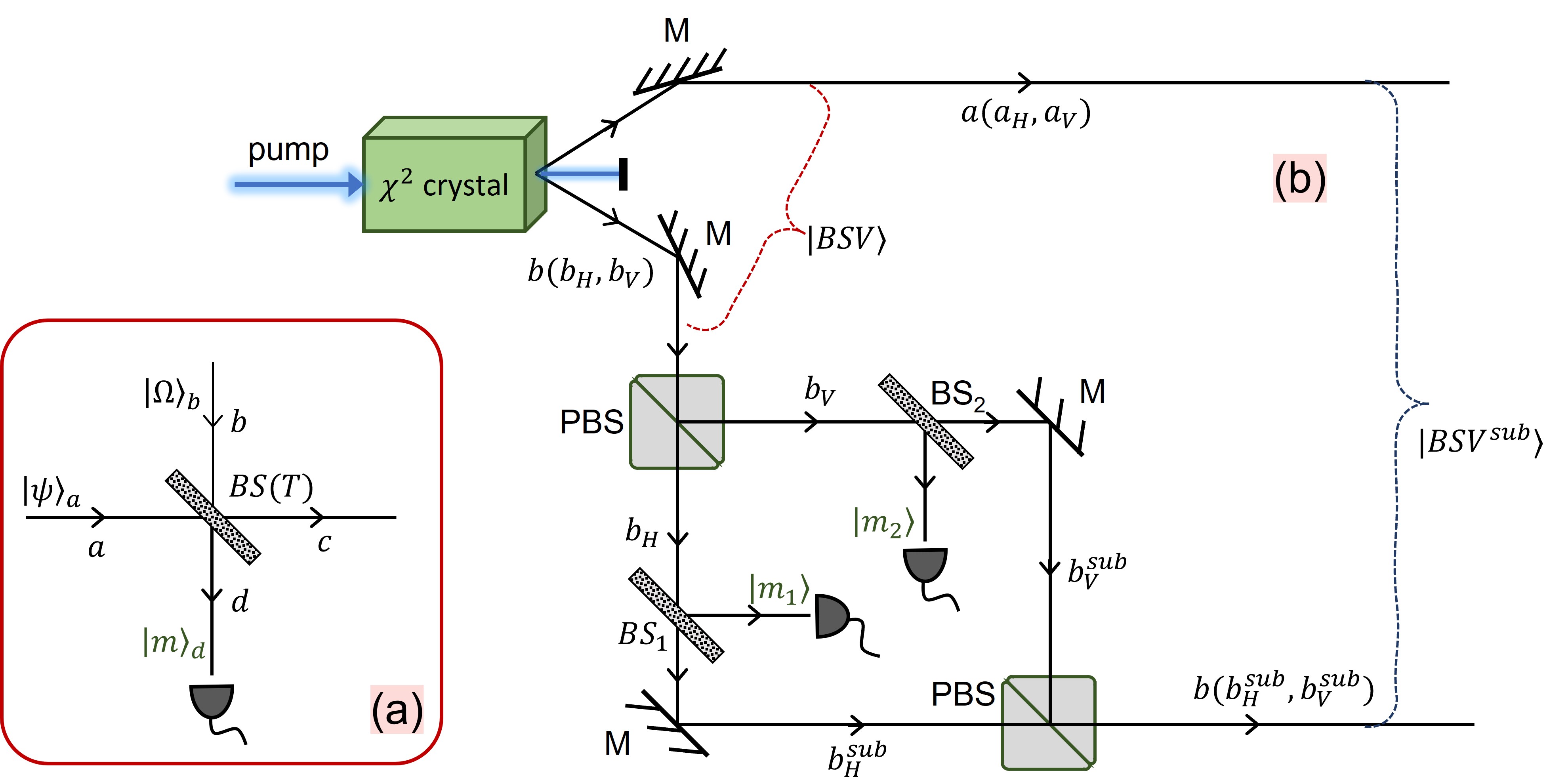
Figure 1: Schematic of photon substraction. Panel (a) shows a subtraction of $m$ photons from an arbitrary state $\ket{\psi}$ feeding the input arm $a$ of a beamsplitter of transmitivity $T$. On the reflected output mode $d$ we place a photon number resolving detector. If $m$ photons are registered then the transmitted mode $c$ contains a state with $m$ photons subtracted. Panel (b): schematic setup to generate non-gaussianity in bright squeezed vacuum with the amplification gain $\Gamma^{\prime}$. Our aim is to subtract $m_{1}$ photons from mode $b_{H}$ and $m_{2}$ photons from mode $b_{V}$ of BSV The beam $b$ impinges on the polarizing beamsplitter (PBS) so that horizontally and vertically polarized photons from $b$ becomes spatially separated, The beams $b_{H}$ and $b_{V}$ pass through the beamsplitters $BS_{1}$ and $BS_{2}$. Once $m_{1}$ and $m_{2}$ photons are detected in the reflected output beams, photon subtracted states in modes $b_{H}^{sub}$ and $b_{V}^{sub}$ generated. Note that such a preparation of BSV leads to to possibility of having an event-ready experiment.

Fig. 1(b) shows how to induce non-gaussianity in BSV. Bright squeezed vacuum is generated via PDC procces. amplification gain is $\Gamma^{\prime}$. The The beam $b$ passes through a polarizing beamsplitter (PBS) that separates spatially modes $b_{H}$ and $b_{V}$. The mode $b_{H}$ impinges on a beamsplitter $BS_{1}$ while the mode $b_{V}$ passes through $BS_{2}$. Both beamsplitters $BS_{1}$ and $BS_{2}$ have the same transmissivity $T$. We place photon numbers resolving detectors on the optical paths of reflected beams. If $m_{1}$ and $m_{2}$ photons are detected we know that the transmitted beams $b_{H}^{sub}$ and $b_{V}^{sub}$ have $m_{1}$ and $m_{2}$ photons subtracted. Finally beams $b_{H}^{sub}$ and $b_{V}^{sub}$ are recombined into $b(b_{H}^{sub},b_{V}^{sub})$ with subtracted photons. The beam $a$ remains unchanged. The output state reads

$$\ket{BSV_{T}^{sub}(\Gamma^{\prime})}$$ (41)

$$= \frac{1}{\sqrt{N_{T}^{sub}(\Gamma^{\prime})}}\sum_{n=m_{1}+m_{2}}^{\infty}\tanh^{n}{\Gamma^{\prime}}\sum_{r=m_{1}}^{n-m_{2}}(-1)^{r}\sqrt{\frac{(n-r)!}{(n-r-m_{2})!}}\sqrt{\frac{r!}{(r-m_{1})!}}(\sqrt{T})^{n-m_{1}-m_{2}}$$

$$\ket{(n-r)_{a_{H}},r_{a_{V}},(r-m_{1})_{b_{H}},(n-r-m_{2})_{b_{V}}},~{}~{}~{}~{}~{}$$

where $N_{T}^{sub}(\Gamma^{\prime})$ is the normalization constant depending on $T$ given by

$$N_{T}^{sub}(\Gamma^{\prime})=\sum_{n=m_{1}+m_{2}}^{\infty}\tanh^{2n}{\Gamma^{\prime}}\sum_{r=m_{1}}^{n-m_{2}}\frac{(n-r)!}{(n-r-m_{2})!}\frac{r!}{(r-m_{V})!}T^{n-m_{1}-m_{2}}.$$ (42)

Let us replace $m_{1}\to m_{V}$, $m_{2}\to m_{H}$, and $\tanh{\Gamma^{\prime}}\to\frac{1}{\sqrt{T}}\tanh{\Gamma}$. Then $N_{T}^{sub}(\Gamma^{\prime})T^{m_{1}+m_{2}}=N^{sub}(\Gamma)$ and in consequence, (41) with subtracted photons and amplification gain $\Gamma^{\prime}$ becomes (29) with the aplification gain $\Gamma$ and added photons. Hence the conclusion that in order to obtain the photon added BSV($\Gamma$), we need to create photon subtracted BSV ($\Gamma^{\prime}$) such that $\tanh{\Gamma}=\tanh{\Gamma^{\prime}}\sqrt{T}$. The use of BSV with unequal number of photons in the beams may facilities the detection of entanglement. Moreover, it has the adventage of an event-ready experiment. The state with $m$ photons added or subtracted is signalized by the detection of these $m$ photons (a detector click).

IV Comparison of entanglement indicators involving variances

We compare our condition (21) with the previous variance condition (9) from Iskhakov et al. (2008) for BSV with (and without) substracted photons. For the simplicity of further comparison we give all separability conditions in the form of $LHS_{sep}\geq RHS_{\hat{X}_{sep}}$ where $LHS$ - the left hand side - remains the same for all the conditions (in its standard or normalized version). The right hand side $RHS_{\hat{X}}$ changes according to the given condition indexed with $\hat{X}$ e.g. $\hat{X}={\Delta(\hat{\Theta}^{AB})^{2}}$ denotes the variance condition (9) for standard Stokes operators etc.

The left hand side for standard Stokes operators is: $LHS=\langle(\hat{\vec{\Theta}}^{A}+\hat{\vec{\Theta}}^{B})^{2}\rangle$. The different right hand sides are given by:

• $RHS_{\Delta(\hat{\Theta}^{AB})^{2}}=2\langle\hat{N}^{A}+\hat{N}^{B}\rangle+\sum_{i=1}^{3}\langle({\hat{\Theta}}_{i}^{A}+{\hat{\Theta}}_{i}^{B})\rangle^{2}$ for (9)

• $RHS_{\Delta(\hat{\Theta}^{AB})^{2}_{{new}}}=RHS_{\Delta(\hat{\Theta}^{AB})^{2}}+\bigg{(}\sqrt{\langle\hat{N}^{A^{2}}\rangle-\langle\hat{\vec{\Theta}}^{A}\rangle^{2}}-\sqrt{\langle\hat{N}^{B^{2}}\rangle-\langle\hat{\vec{\Theta}}^{B}\rangle^{2}}\bigg{)}^{2}$ for our (21)

We use the same reasoning for normalized Stokes operators.

We define $\kappa=LHS-RHS_{\hat{X}}$. We For any separable state $\kappa_{sep}\geq 0$. If $\kappa<0$, the state in question is entangled. The more negative $\kappa$ is, the more efficient is detection of entanglement.

Let us first analyze if using our modified entanglement condition applied to BSV with one horizontally polarized photon subtracted has any adventage at all over using its ”basic” version i.e. the condition involving variances from Iskhakov et al. (2008) and BSV. Fig. 2 shows $\kappa(\Gamma)$ for these scenarios for standard (see the subfigure on the left) and normalized Stokes operators (the subfigure on the right). On the left side of fig. 2 we find $\kappa(\Gamma)$ for condition (21) applied to non-gaussian BSV put together with $\kappa(\Gamma)$ for condition 9 and “regular” BSV for standard Stokes operators. Our modified scenario leads to stronger detection of entanglement. Then, on the right side of 2 we have similar plots for normalized Stokes operators (we compare conditions 10 for BSV and 27 for non-gaussain BSV). Concerning normalized Stokes operators for low values of $\Gamma$ it is more advantageous to use the “basic” scenario with (10) than to add one photon from BSV and use our condition (27).

In the main text we concentrate on standard Stokes operators for which the analytical expressions for $LHS$ and all $RHS_{\hat{X}}$ are given in appendix A. The corresponding plots and formulas for normalized Stokes operators can be found in appendix B.

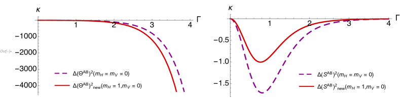
Figure 2: Plots of c$\kappa$ in function of amplification gain $(\Gamma)$. On the left: comparison of conditions (9) applied for BSV and (21) for non-gaussian BSV (with one photon horizontally polarized $m_{H}=1$ subtracted) for standard Stokes operators. On the right analogous comparison of (10) and (27). The photon addition combined with the use of our condition helps in entanglement detection only for standard Stokes operators.

Now let us check the behaviour of analyzed entanglement conditions when they are both applied to BSV with different numbers added photons. Fig. 3 shows the values of $\kappa$ in function of the amplification gain $\Gamma$ for condition (9) and (21). We checked that as we increase the difference of total number of photons between the beams (by subtracting $m_{H}$ and or $m_{V}$ to one beam), the additional non-negative term in $RHS_{\Delta(\hat{\Theta}^{AB})^{2}_{{new}}}$ of (21) gets more impact on lowering the value of $\kappa$. As expected we noted that condition (9) is unable to capture entanglement if we subtract (or add) photons from BSV for low values of $\Gamma$, We did not put results for subtracting more than 2 photons in the beam because the obtained results are conceptually similar to the cases $m_{H}$ and $m_{V}\in\{0,1\}$.

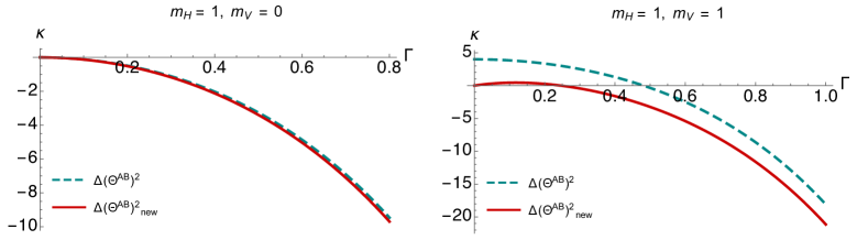
Figure 3: Plots of $\kappa$ in function of amplification gain $(\Gamma)$. for conditions (9) and (21) for BSV with $m_{H}$ and $m_{V}\in\{0,1\}$ photons added. Note the adventage of our condition (21) - entanglement can be observed for smaller value of amplification gain $(\Gamma\approx 0.2)$ than for (9)

V Conclusions

More optimal conditions for optical fields tailored for states with undefined number of photons were proposed. Our conditions, based on polarization measurement, involve variances and hence they have clear physical interpretation - the spread of data around the mean value define the nature of correlations. If for the given state the spread of the data results smaller than it is assumed for separable states, the given state is entangled. We compared the efficiency of entanglement detection with our condition versus other known entanglement condition based on variances for bright squeezed vacuum and bright squeezed vacuum with added photons. We also analyzed the equivalency of adding and subtracting photons in bright squeezed vacuum and proposed an experimental scheme to perform such experiments. Our scheme leads event-ready detection of entanglement for BSV. We have shown that by applying our conditions to non-gaussian bright squeezed vacuum, we can obtain stronger entanglement detection. However, that statement refers only to standard Stokes operators. For normalized Stokes operators adding photons to BSV and using our condition does not improve entanglement detection compared to other studies cases.

Appendix A Explicit formulas used in the comparison of entanglement conditions for standard Stokes operators

We give the analytical form of the formulas for $LHS$ and $RHS_{\hat{X}}$ for (9) and (21). The left hand side, the same for all conditions, boils down to

$$LHS=(m_{H}+m_{V}+1)^{2}-1.$$ (43)

Note that $LHS$ does not depend on $\Gamma$, which is not surprising because for if no photon are added the $LHS=0$, due to perfect EPR anticorrelations of BSV. Then, to calculate the right hand sides $(RHS_{\hat{X}})$ we need the following components:

$$\langle\hat{N}^{B}\rangle_{add}=(m_{H}+m_{V}+2)\sinh^{2}\Gamma,$$ (44)

$$\langle\hat{N}^{A^{2}}\rangle_{add}=\sinh^{2}\Gamma(m_{H}+m_{V}+2)\left(1+\sinh^{2}\Gamma(m_{H}+m_{V}+3)\right),$$ (45)

$$\langle\hat{\Theta}_{3}^{A}\hat{\Theta}_{3}^{B}\rangle_{add}=-\frac{1}{2}(1+m_{H})(1+m_{V})\sinh^{2}(2\Gamma),$$ (46)

$$\langle\hat{N}^{A}\hat{N}^{B}\rangle_{add}=(m_{H}+m_{V}+2)\cosh^{2}\Gamma\sinh^{2}\Gamma(1+m_{H}+m_{V}+2\tanh^{2}\Gamma).$$ (47)

Note that after introducing extra photons BSV ceases to be rotationally invariant (with respect to the same rotations of both observers). We still have: $\langle\hat{\Theta}_{1}^{X}\rangle_{add}=\langle\hat{\Theta}_{2}^{X}\rangle_{add}=0$, for $X=A,B$, but

$$\langle\hat{\Theta}_{3}^{A}\rangle_{add}-(m_{H}-m_{V})\sinh^{2}{\Gamma}.$$ (48)

The formulas listed above were used to obtain plots on fig. 2 and fig.3 in the main text.

Appendix B Comparison of entanglement conditions for normalized Stokes operators and conditions involving variances.

Figure 4: The plots of $\kappa(\Gamma)$ for (10) and 27 for different amount of added photons $m_{H_{(V)}}$.

We repeat the reasoning form the begining of section IV in the main text for normalized Stokes parameters. We have :

$$LHS_{\hat{S}^{AB}}=\sum_{i=1}^{3}\langle({\hat{S}}_{i}^{A}+{\hat{S}}_{i}^{B})^{2}\rangle,$$ (49)

as well as:

• $RHS_{\Delta(\hat{S}^{AB})^{2}}=2\langle\hat{\Pi}^{A}\frac{1}{\hat{N}^{A}}\hat{\Pi}^{A}+\hat{\Pi}^{B}\frac{1}{\hat{N}^{B}}\hat{\Pi}^{B}\rangle+\sum_{i=1}^{3}\langle({\hat{S}}_{i}^{A}+{\hat{S}}_{i}^{B})\rangle^{2},$ for (10)

• $RHS_{\Delta(\hat{S}^{AB})^{2}_{{new}}}=RHS_{\Delta(\hat{S}^{AB})^{2}}+\bigg{(}\sqrt{\langle\hat{\Pi}^{A^{2}}\rangle-\langle\hat{\vec{S}}^{A}\rangle^{2}}-\sqrt{\langle\hat{\Pi}^{B^{2}}\rangle-\langle\hat{\vec{S}}^{B}\rangle^{2}}\bigg{)}^{2}$ for 27

.

The formulas for probability of non-vacuum events go as follows:

$$\langle\hat{\Pi}^{A}\rangle_{add}=1-(\sech^{2}{\Gamma})^{m_{H}+m_{V}+2}$$ (50)

and

$$\langle\hat{\Pi}^{B}\rangle_{add}=1-\delta_{m_{H},0}\delta_{m_{V},0}(\sech^{2}{\Gamma})^{2},$$ (51)

For any $m_{H}$ and $m_{V}$ we have $\langle\hat{S}_{1}^{X}\rangle_{add}=\langle\hat{S}_{2}^{X}\rangle_{add}=0$ for $X=A,B$. Moreover if $m_{H}=m_{V}$ also $\langle\hat{S}_{3}^{A}\rangle_{add}=\langle\hat{S}_{3}^{B}\rangle_{add}=0$. For all the rest of the cases we get

$$\langle\hat{S}_{3}^{A}\rangle_{add}=\frac{m_{H}-m_{V}}{m_{H}+m_{V}+2}\Big{(}1+\frac{2\sech^{2}\Gamma(m_{H}+m_{V}+\sech^{2}\Gamma)}{(m_{H}+m_{V})(m_{H}+m_{V}+1)}\Big{)},$$ (52)

$$\langle\hat{S}_{3}^{B}\rangle_{add}=-\frac{(m_{H}-m_{V})(1-(\sech^{2}\Gamma)^{2(m_{H}+m_{V}+2)})}{m_{H}+m_{V}+2},$$ (53)

$m_{H}$	$m_{V}$	$\langle\hat{\Pi}^{B}\frac{1}{\hat{N}_{B}}\hat{\Pi}^{B}\rangle_{add}$	$\langle\hat{S}_{3}^{A}\hat{S}_{3}^{B}\rangle_{add}$	$\langle\hat{S}_{1}^{A}\hat{S}_{1}^{B}\rangle_{add}$
1	0	$\frac{1}{2}\big{(}\sinh^{2}\Gamma\left(\cosh^{2}\Gamma+3\right)-2\log\left(\sech^{2}\Gamma\right)\big{)}\sech^{6}\Gamma$	$\frac{1}{3}\big{(}3\sech^{6}\Gamma-\sech^{4}\Gamma-\sech^{2}\Gamma-1\big{)}$	$\frac{1}{3}\big{(}3\sech^{6}\Gamma-\sech^{4}\Gamma-\sech^{2}\Gamma-1\big{)}$
1	1	$\frac{1}{96}\sech^{8}\Gamma\big{(}87\cosh(2\Gamma)+12\cosh(4\Gamma)+\cosh(6\Gamma)-96\log\left(\sech^{2}\Gamma\right)-100\big{)}$	$\frac{1}{15}\big{(}6\sech^{8}\Gamma-\sech^{4}\Gamma-2\sech^{2}\Gamma-3\big{)}$	$\frac{2}{15}\big{(}6\sech^{8}\Gamma-\sech^{4}\Gamma-2\sech^{2}\Gamma-3\big{)}$

Table 1: Formulas needed to calculate $RHS$ for entanglement conditions with normalized Stokes operators.

We were not able to find a concise formulas for arbitrary $m_{H}$ and $m_{V}$ for other expressions we give their specific values of $m_{H}$ and $m_{V}\in\{0,1\}$ in the table 1.

Fig 4 refers to conditions (10) and (27) for normalized Stokes operators and non-gaussian BSV. The more photons we add, the bigger is the gap between $\kappa(\Gamma)$ for these conditions.