Delayed Reinforcement Learning by Imitation

Abstract

When the agent’s observations or interactions are delayed, classic reinforcement learning tools usually fail. In this paper, we propose a simple yet new and efficient solution to this problem. We assume that, in the undelayed environment, an efficient policy is known or can be easily learned, but the task may suffer from delays in practice and we thus want to take them into account. We present a novel algorithm, Delayed Imitation with Dataset Aggregation (DIDA), which builds upon imitation learning methods to learn how to act in a delayed environment from undelayed demonstrations. We provide a theoretical analysis of the approach that will guide the practical design of DIDA. These results are also of general interest in the delayed reinforcement learning literature by providing bounds on the performance between delayed and undelayed tasks, under smoothness conditions. We show empirically that DIDA obtains high performances with a remarkable sample efficiency on a variety of tasks, including robotic locomotion, classic control, and trading.

1 Introduction

In reinforcement learning (RL), it is generally assumed that the effect of an action over the environment is known instantaneously to the agent. However, in the presence of delays, this classic setting is challenged. The effect of a delayed action execution or state observation, if not accounted for, can have perilous effects in practice (Dulac-Arnold et al., 2019). It can induce a performance loss in trading (Wilcox, 1993), create instability in dynamic systems (Dugard & Verriest, 1998; Gu & Niculescu, 2003), be detrimental to the training of real-world robots (Mahmood et al., 2018). To further grasp the importance of delay, one may notice that most traffic laws around the world base safety distances on drivers’ “reaction time”, which is partly due to the perception of the event and partly to the implementation of the action (Droździel et al., 2020). These two types of delay have an exact correspondence in RL, where they are dubbed as state observation and action execution delays. There are many ways in which delays can further vary. They may be anonymous (i.e., not known to the agent), constant or stochastic, integer or non-integer. In this work, as in most of the literature, we focus on constant non-anonymous delays in the action execution or, equivalently (Katsikopoulos & Engelbrecht, 2003), in the state observation.

Previous research can be divided into three main directions. In memoryless approaches the agent’s policy depends on the last observed state (Schuitema et al., 2010). Augmented approaches try to cast the problem into a Markov decision process (MDP) by building policies based on an augmented state, composed of the last observed state and on the actions that the agent knows it has taken since then (Bouteiller et al., 2020). A last line of research, which we refer to as model-based approach, considers using as a policy input any statistics about the current unknown state that can be computed from the augmented state (Walsh et al., 2009; Firoiu et al., 2018; Chen et al., 2021; Agarwal & Aggarwal, 2021; Derman et al., 2021; Liotet et al., 2021). The goal of this approach is to avoid the curse of dimensionality posed by the augmented state (Walsh et al., 2009; Bouteiller et al., 2020). We formalize the problem of delays in Section 3 and give a more in-depth description of the literature in Section 4.

We adopt the simple yet practically effective idea of learning a policy in a delayed environment by applying imitation learning to a policy learned in the undelayed environment, as described in Section 5. Not any imitation learning algorithm would work to this aim and DAgger (Ross et al., 2011) is particularly well suited for being one of the few algorithms to compute the loss under the learner’s own distribution (Osa et al., 2018), which is important due to the shift in distribution induced by the delay. We provide a theoretical analysis (Section 6) which, under smoothness conditions over the MDP, bounds the performance lost by introducing delays. Finally, we provide an extensive experimental analysis (Section 7) where our algorithm is compared with state-of-the-art approaches on a variety of delayed problems and demonstrates great performances and sample efficiency.

2 Preliminaries

Reinforcement Learning   A discrete-time discounted Markov Decision Process (MDP) (Puterman, 2014) is a 6-tuple $\mathcal{M}=(\mathcal{S},\mathcal{A},p,R,\gamma,\mu)$ where $\mathcal{S}$ and $\mathcal{A}$ are measurable sets of states and actions respectively, $p(s^{\prime}|s,a)$ is the probability to transition to a state $s^{\prime}$ departing from state $s$ and taking action $a$, $R(s,a)$ is a random variable defining the reward collected during such a transition. We denote by $r(s,a)$ its expected value. Finally, $\mu$ is the initial state distribution. The agent’s goal is to find a policy $\pi$, which assigns probabilities to the actions given a state, to maximize the expected discounted return with discount factor $\gamma\in[0,1)$, defined as

$$J(\pi)=\operatorname*{\mathbb{E}}_{\begin{subarray}{c}s_{t+1}\sim p(\cdot|s_{t},a_{t})\\ a_{t}\sim\pi(\cdot|s_{t})\\ s_{0}\sim\mu(\cdot)\end{subarray}}\left[\sum_{t=0}^{H}\gamma^{t}R(s_{t},a_{t})\right].$$ (1)

We consider an infinite horizon setting, where $H=\infty$. Note that $\frac{1}{1-\gamma}$ can be seen as the effective horizon in this case. We restrict the set of policies to the stationary Markovian policies, $\Pi$, as it contains the optimal one (Puterman, 2014). RL analysis frequently introduces the concept of state-action value function, which quantifies the expected return obtained under some policy, starting from a given state and fixing the first action. Formally, this function is defined as

$$Q^{\pi}(s,a)=\operatorname*{\mathbb{E}}_{\begin{subarray}{c}a_{t}\sim\pi(\cdot|s_{t})\end{subarray}}\left[\sum_{t=0}^{H}\gamma^{t}R(s_{t},a_{t})\bigg{|}\begin{subarray}{c}s_{0}=s,\\ a_{0}=a\end{subarray}\right].$$ (2)

Similarly we define the state value function as $V^{\pi}(s)=\operatorname*{\mathbb{E}}_{a\sim\pi(\cdot|s)}[Q^{\pi}(s,a)]$. Lastly, we consider the discounted visited state distribution under some policy $\pi$, starting from any initial distribution $\rho$, for some state $s\in\mathcal{S}$ as

$$d_{\rho}^{\pi}(s)=(1-\gamma)\sum_{t=0}^{\infty}\gamma^{t}\operatorname*{\mathbb{P}}(s_{t}=s|\pi,\rho).$$

Lipschitz MDPs  We now introduce notions that will allow us to characterize the smoothness of an MDP. Let $L>0$ and let $(X,\operatorname{\text{d}}_{X})$ and $(Y,\operatorname{\text{d}}_{Y})$ be two metric spaces. A function $f:X\rightarrow Y$ is said to be $L$-Lipschitz continuous ($L$-LC) if, $\forall x,x^{\prime}\in X$, $\operatorname{\text{d}}_{Y}(f(x),f(x^{\prime}))\leq L\operatorname{\text{d}}_{X}(x,x^{\prime})$. We denote the Lipschitz semi-norm of a function $f$ as $\left\|f\right\|_{L}=\sup_{x,x^{\prime}\in X,x\neq x^{\prime}}\frac{\operatorname{\text{d}}_{Y}(f(x),f(x^{\prime}))}{\operatorname{\text{d}}_{X}(x,x^{\prime})}$. In real space $X\subset\mathbb{R}^{n}$, we use as distance the Euclidean one, i.e., $\operatorname{\text{d}}_{X}(x,x^{\prime})=\lVert x-x^{\prime}\rVert_{2}$. As for the probabilities, we use the $L_{1}$-Wasserstein distance, which for some probabilities $\mu,\nu$ with sample space $\Omega$ is (Villani, 2009):

$$\mathcal{W}_{1}(\mu,\nu)=\sup_{\left\|f\right\|_{L}\leq 1}\left|\int_{\Omega}f(\omega)(\mu-\nu)(d\omega)\right|.$$

We now use those concepts to quantify the smoothness of an MDP.

Definition 2.1 (Lipschitz MDP).

An MDP is said to be $(L_{P},L_{r})$-LC if, for all $(s,a),(s^{\prime},a^{\prime})\in\mathcal{S}\times\mathcal{A}$

$$\mathcal{W}_{1}(p(\cdot|s,a),p(\cdot|s^{\prime},a^{\prime}))\leq L_{P}\left(\operatorname{\text{d}}_{\mathcal{S}}(s,s^{\prime})+\operatorname{\text{d}}_{\mathcal{A}}(a,a^{\prime})\right),$$

$$\left|r(s,a)-r(s^{\prime},a^{\prime})\right|\leq L_{r}\left(\operatorname{\text{d}}_{\mathcal{S}}(s,s^{\prime})+\operatorname{\text{d}}_{\mathcal{A}}(a,a^{\prime})\right).$$

Definition 2.2 (Lipschitz policy).

A stationary Markovian policy $\pi$ is said to be $L_{\pi}$-LC if, $\forall s,s^{\prime}\in\mathcal{S}$

$$\mathcal{W}_{1}(\pi(\cdot|s),\pi(\cdot|s^{\prime}))\leq L_{\pi}\operatorname{\text{d}}_{\mathcal{S}}(s,s^{\prime}).$$

These concepts provide useful tools for theoretical analysis and have been extensively used in the field of RL (Rachelson & Lagoudakis, 2010). Under the assumption of $(L_{P},L_{r})$-LC MDP and $L_{\pi}$-LC policy $\pi$, provided that $\gamma L_{P}(1+L_{\pi})\leq 1$, then $Q^{\pi}$ is $L_{Q}$-LC with $L_{Q}=\frac{L_{r}}{1-\gamma L_{P}(1+L_{\pi})}$ (Rachelson & Lagoudakis, 2010, Theorem 1). This property can be useful to prove the Lipschitzness of the $Q$ function.

Additionally, in the case of delays, the smoothness of trajectories (sequence of consecutive states and actions) is a key factor. Intuitively, smoother trajectories make the current unknown state more predictable. Therefore, we consider the concept of time-Lipschitzness, introduced by Metelli et al. (2020).

Definition 2.3 (Time-Lipschitz MDP).

An MDP is said to be $L_{T}$-Time Lipschitz Continuous ($L_{T}$-TLC) if, $\forall s,a\in\mathcal{S}\times\mathcal{A}$

$$\mathcal{W}_{1}(p(\cdot|s,a),\delta_{s})\leq L_{T},$$

where $\delta_{s}$ is the Dirac distribution with mass on $s$.

3 Problem definition

A delayed MDP (DMDP) stems from an MDP endowed with a sequence of variables $(\Delta_{t})_{t\in\mathbb{N}}$ corresponding to the delay at each step of the sequential process. The delay can affect the state observation, which implies that the agent has no access to the current state but only to a state visited $\Delta_{t}$ steps before. Affecting the action execution, the delay implies that the agent must select an action that will be executed $\Delta_{t}$ steps from now. Lastly, reward collection delays may raise credit assignment issues and are outside the scope of this paper. In any case, the DMDP violates the Markov assumption since the next observed state-reward couple does not depend only on the currently observable state and the chosen action. In the literature, the delay is usually assumed to be a Markovian process, that is $\Delta_{t}\sim P(\cdot|\Delta_{t-1},s_{t-1},a_{t-1})$. Note that this definition includes state dependent delays when $\Delta_{t}\sim P(\cdot|s_{t-1})$, Markov chain delays when $\Delta_{t}\sim P(\cdot|\Delta_{t-1})$ and stochastic delays when $(\Delta_{t})_{t\in\mathbb{N}}$ are i.i.d.

In this work we consider constant delays, denoting the delay with the symbol $\Delta$. When the delay is constant, the action execution delay and the state observation one are equivalent (Katsikopoulos & Engelbrecht, 2003), thus, it is sufficient to consider only the state observation delay. Furthermore, following Katsikopoulos & Engelbrecht (2003), we consider a reward collection delay equal to the state observation delay so as not to collect a reward on a yet unobserved state, which could result in some form of partial state information. Finally, we assume that the delay is known to the agent, placing ourselves in the non-anonymous delay framework.

Within this reduced framework, it is possible to introduce an important concept of DMDPs, the augmented state. Given the last observed state $s$ and the sequence of actions $(a_{1},\dots,a_{d})$ which have been taken since then, but whose outcome has not yet been observed, the agent can construct an augmented state, i.e., a new state in $\mathcal{X}=\mathcal{S}\times\mathcal{A}^{\Delta}$ which casts the DMDP into an MDP (Bertsekas, 1987; Altman & Nain, 1992). Said alternatively, the augmented state contains all the information the agent needs to learn the optimal policy in the DMDP. From the augmented state, we can gather information on the current state. This information can be summarized by the belief, the probability distribution of the current unknown state $s$ given the augmented state $x$ as $b(s|x)$. More explicitly, given $x=(s_{1},a_{1},\dots a_{\Delta})$, one has

$$b(s|x)=\int_{S^{\Delta-1}}p(s|s_{\Delta},a_{\Delta})\prod_{i=2}^{\Delta}p(s_{i}|s_{i-1},a_{i-1})ds_{i}.$$

The delayed reward collected for playing action $a$ on $x$ is given by $\widetilde{r}(x,a)=\operatorname*{\mathbb{E}}_{\begin{subarray}{c}s\sim b(\cdot|x)\end{subarray}}\left[r(s,a)\right]$. To complete the DMDP framework, we define $\widetilde{\mu}$, the initial augmented state distribution. It samples the state contained in the augmented state under $\mu$ and samples the first action sequence under a distribution whose choice depends on the environment. We consider a uniform distribution on $\mathcal{A}$.

4 Related works

The first proposed solution to the problem of delays is to use regular RL algorithms on the augmented-state MDP. Although the optimal delayed policy could potentially be obtained, this approach is affected by the exponential growth of the augmented state space, which becomes $|\mathcal{S}||\mathcal{A}|^{\Delta}$ (Walsh et al., 2009) and is a source of the curse of dimensionality that is harmful in practice. Nonetheless, recent work by Bouteiller et al. (2020) revisits this approach and propose a clever way to resample trajectories without interacting with the environment by populating the augmented state with actions from a different policy, greatly improving the sample efficiency. They propose an algorithm, Delay-Correcting Actor-Critic (DCAC), which builds on SAC (Haarnoja et al., 2018) using the aforementioned resampling idea. DCAC has great experimental results and is sample efficient by design.

A second line of research focuses on memoryless policies, inspired by the partially observable MDP literature. It ignores the action queue to act according to the last observed state only. However, the delay can still be taken into account as in dSARSA (Schuitema et al., 2010), a modified version of SARSA (Sutton & Barto, 2018) which accounts for the delay during its update. Indeed, SARSA would credit the reward collected for applying action $a$ on the augmented state $x$, containing the last observed state $s$, to the pair $(s,a)$. Instead, dSARSA proposes to credit $(s,a_{1})$, where $a_{1}$ is the oldest action stored in $x$, the action actually applied on $s$. Despite being memoryless, dSARSA achieves great performances in practice.

Finally, the most common line of research, the model-based approach, relies on computing statistics on the current state which are then used to select an action. The name model-based comes from the fact that those solutions usually learn a model of the environment to predict the current state, by simulating the effect of the actions stored in the augmented state on the last observed state. Walsh et al. (2009) learn the transition as a deterministic mapping so as to predict the most probable state, before selecting actions based on it. Derman et al. (2021) and Firoiu et al. (2018) propose a similar approach by learning the transitions with feed-forward and recurrent neural networks, respectively. Agarwal & Aggarwal (2021) estimate the transition probabilities and the undelayed $Q$ function to select the action that gives the maximum $Q$ under the estimated distribution of the current state. Chen et al. (2021) use a particle-based approach to produce potential outcomes for the current state and, interestingly, extend the predictions to collect better value estimates. Liotet et al. (2021) propose D-TRPO which learns a vectorial encoding of the belief of the current state itself which is then used as an input to the policy, the latter being trained with TRPO (Schulman et al., 2015a). The authors also propose another algorithm, L2-TRPO which, instead of the belief, learns the expected current state by minimizing the predicted and the real state under the $l^{2}$-norm.

While most of these works assume that the delay is fixed, some consider the problem of stochastic delays (Bouteiller et al., 2020; Derman et al., 2021; Agarwal & Aggarwal, 2021). Only one of them considers the case of non-integer delays (Schuitema et al., 2010).

5 Imitation Learning for Delays

Our proposed approach is motivated by the limitations of two lines of research from the literature. Augmented approaches are affected by the curse of dimensionality that hinders the learning process, while model-based approaches require carefully designed models of the state transitions and usually involve a computational burden. Instead, we propose to learn a mapping from augmented state directly to undelayed expert actions, facilitating the learning process as opposed to augmented approaches and by removing explicit approximation of transitions as opposed to model-based approaches. Our approach, however, implies that learning is split into two sub-problems: learning an expert undelayed policy and then imitating this policy in a DMDP.

5.1 Imitation Learning

It is usually easier to learn a behavior from demonstrations than learning from scratch using standard RL techniques. Imitation learning aims at learning a policy by mimicking the actions of an expert, bridging the gap between RL and supervised learning. Obviously, it requires that one can collect examples of an expert’s behavior to learn from. For an expert policy $\pi_{E}$, most imitation learning approaches aim at finding a policy $\pi$ that minimizes $\operatorname*{\mathbb{E}}_{s\sim d_{\mu}^{\pi_{E}}}[l(s,\pi)]$ (Ross et al., 2011) where $l(s,\pi)$ is a loss designed to make $\pi$ closer to $\pi_{E}$. Note that this objective is defined under the state distribution induced by $\pi_{E}$. This can easily be problematic as, whenever the learner makes an error, it could end up in a state where its knowledge of the expert’s behavior is poor and therefore errors could accumulate. Indeed, it has been shown that the error made by the learner potentially propagates as the squared effective horizon as shown in (Xu et al., 2020, Theorem 1). This is consistent with other bounds found in the literature depending on $H^{2}$ in the finite horizon setting (Ross & Bagnell, 2010, Theorem 2.1).

One successful solution to this problem is dataset aggregation as proposed by Ross et al. (2011) in their DAgger algorithm. The idea is to sample new data under the learned policy and query the expert on those new samples in order to match the learner’s state distribution. DAgger recursively builds a dataset $\mathcal{D}$ by sampling trajectories under policy $\pi_{i}=\beta_{i}\pi_{E}+(1-\beta_{i})\hat{\pi}_{i}$ obtained from a $\beta_{i}$-weighted mixture of the expert policy and the previously imitated policy $\hat{\pi}_{i}$. One then queries the expert’s policy on the states encountered in these trajectories and adds those tuples $(s,\pi_{E}(s))$ to $\mathcal{D}$. Finally, a new imitated policy $\hat{\pi}_{i+1}$ is trained on $\mathcal{D}$. The sequence $(\beta_{i})_{i\in[\![1,N]\!]}$ is such that $\beta_{1}=1$, so as to sample initially only from $\pi_{E}$ and $\beta_{N}=0$ to sample only from the imitated policy in the end.

5.2 Duality of Trajectories

Once sampled, the trajectories, either from a DMDP or its underlying MDP, can be interpreted in both processes when the delay is an integer number of steps. In a DMDP, the current state will eventually be observed by a delayed agent. In an MDP, the trajectories can be re-organized to simulate the effect of a delay. In particular, this means that one can collect trajectories with an undelayed environment and sample either from an undelayed policy or a delayed policy (by creating a synthetic augmented state). This is exactly what is required to adapt DAgger to imitate an undelayed expert with a delayed learner.

Algorithm 1 Delayed Imitation with DAgger (DIDA)

Inputs undelayed environment $\mathcal{E}$, undelayed expert $\pi_{E}$, $\beta$ routine, number of steps $N$, empty dataset $\mathcal{D}$.
Outputs: delayed policy $\pi_{I}$

1:  for $\beta_{i}$ in $\beta$-routine do

2:     for $j$ in $\{1,\dots,N\}$ do

3:        if New episode then

4:           Initialize state buffer $(s_{1},s_{2},\dots,s_{\Delta})$ and action buffer $(a_{1},a_{2}\dots,a_{\Delta-1})$

5:        end if

6:        Sample $a_{E}\sim\pi_{E}(\cdot|{{s}}_{\Delta})$, set $a=a_{E}$

7:        if Random $u\sim U([0,1])\geq\beta_{i}$ then

8:           Overwrite ${a\sim\pi_{I}(\cdot|[{s}_{1},a_{1},\dots,a_{\Delta-1}])}$

9:        end if

10:        Aggregate dataset: $\qquad\mathcal{D}\leftarrow\mathcal{D}\cup([{s}_{1},a_{1},\dots,a_{\Delta-1}],a_{E})$

11:        Apply $a$ in $\mathcal{E}$ and get new state $s$

12:        Update buffers: $\qquad({s}_{1},\dots,{s}_{\Delta})\leftarrow({s}_{2},\dots,{s}_{\Delta},s)$ $\qquad({a}_{1},\dots,{a}_{\Delta-1})\leftarrow({a}_{2},\dots,{a}_{\Delta-1},a)$

13:     end for

14:     Train $\pi_{I}$ on $\mathcal{D}$

15:  end for

5.3 Imitating an Undelayed Policy

We follow the learning scheme of DAgger with the slight difference that, if the expert is queried, then the current state is fed to $\pi_{E}$ while if the imitator policy is queried, an augmented state is built from the past samples, considering the state $\Delta$-steps before the current state and the sequence of actions taken since then. This implies that a buffer of the latest states and actions has to be built. We present our approach, which we call Delayed Imitation with DAgger (DIDA), in Algorithm 1. In practice there is no need to store each augmented state in the dataset $\mathcal{D}$ since most of the actions contained inside one are also contained in others. Therefore, only trajectories of state and action can be stored, from which augmented states are recreated during the training of $\pi_{I}$.

What will the policy learned by DIDA be in practice? Given an augmented state $x$, DIDA learns to replicate the action taken by the expert on the current state $s$, unknown to the agent. However, the same augmented state can lead to different current states, which is summarized in the belief $b(s|x)$. Therefore, DIDA learns the following policy

$$\widetilde{\pi}_{b}(a|x)=\int_{\mathcal{S}}b(s|x)\pi_{E}(a|s)ds.$$ (3)

The learned policy is therefore similar to the policies from model-based approaches, and, for this reason, may yield sub-optimal policies in some MDPs (Liotet et al., 2021, Proposition VI.1.). In practice, the class of functions of the imitated policy $\pi_{I}$ and the loss chosen for training in step 15 of Algorithm 1 may slightly modify the policy learned by DIDA. For instance, a deterministic $\pi_{I}$ would naturally forbid to learn the distribution given in Equation 3. This is discussed in Section D.1.

5.4 Extension to non integer delays

We now suppose that the delay is non-integer, yet still constant. For simplicity, we assume $\Delta\in(0,1)$ but the general case follows from similar considerations. We consider a $\Delta$-delay in the action execution (the case of state observation is similar).

DMDP with non-integer delays can be viewed as the result of two interleaved MDPs, $\mathcal{M}$ with time indexes $t,t+1,\dots$ and $\mathcal{M}_{\Delta}$ with indexes $t+\Delta,t+\Delta+1,\dots$. Those two discrete MDPs stem from a single continuous process, of which we observe only some fixed time steps, similarly to (Sutton et al., 1999). They share the same transition and reward functions. A delayed agent would see states from $\mathcal{M}$ while executing actions on states of $\mathcal{M}_{\delta}$. In practice, the agent taking action $a_{t}$ seeing state $s_{t}$ would collect a reward $r(s_{t+\Delta},a_{t})$. The transition probabilities are also affected. We define $b_{\Delta}(s_{t+\Delta}|s_{t},a)$ the probability of reaching $s_{t+\Delta}$ from $s_{t}$ when action $a$ is applied during time $\Delta$ and $b_{1-\Delta}(s_{t}|s_{t-1+\Delta},a)$ the probability of reaching $s_{t+\Delta}$ from $s_{t}$ when action $a$ is applied during time $1-\Delta$. To make the definition consistent with the regular MDP, those probabilities must satisfy that, for all $(s,a,s^{\prime})\in\mathcal{S}\times\mathcal{A}\times\mathcal{S}$

$$p(s^{\prime}|s,a)=\int_{\mathcal{S}}b_{1-\Delta}(s^{\prime}|z,a)b_{\Delta}(z|s,a)~{}dz.$$ (4)

Clearly, even for $\Delta\in(0,1)$, an augmented state $x_{t}=(s_{t},a_{t-1})\in\mathcal{S}\times\mathcal{A}\eqqcolon\mathcal{X}$ is needed in order not to lose information about the state $s_{t+\Delta}\sim b_{\Delta}(\cdot|s_{t},a_{t-1})$. The DMDP with augmented state can again be cast into an MDP as in Bertsekas (1987); Altman & Nain (1992), where the new transition is defined for $x_{t}=(s_{t},a_{t-1}),x_{t+1}=(s_{t+1},a_{t})\in\mathcal{X}$,

$$\tilde{p}(x_{t+1}|x_{t},a)\coloneqq\delta_{a}(a_{t})\int_{\mathcal{S}}b_{1-\Delta}(s_{t+1}|z,a)b_{\Delta}(z|s_{t},a_{t-1})~{}dz,$$

where the term $\delta_{a}(a_{t})$ ensures that the new extended state contains the action that has been applied on $x_{t}$. For delays greater than 1, one needs to consider the augmented state in the space $\mathcal{S}\times\mathcal{A}^{\lceil\Delta\rceil}$ and the previous considerations hold by first considering the integer part of the delay and then its remaining non-integer part. In this setting, we propose to use DIDA by learning an undelayed policy in $\mathcal{M}_{\Delta}$ and imitating it by building an augmented state from the states in $\mathcal{M}$.

6 Theoretical analysis of the approach

We will now provide a theoretical analysis of the approach proposed above. The role of this analysis is twofold. First, it gives insights into which expert undelayed policy is best suited to be imitated in a DMDP. Secondly, it provides general results on the value functions bounds between DMDPs and MDPs, when the latter has guarantees of smoothness, setting aside pathological counterexamples such as in (Liotet et al., 2021, Proposition VI.1.) while remaining realistic. To compare the performance of delayed and undelayed policies, we have to compare the corresponding state value functions, which is non trivial, since they live on two different spaces ($\mathcal{S}$ and $\mathcal{X}=\mathcal{S}\times\mathcal{A}^{\Delta}$).

Different approaches were proposed to address this issue. In (Walsh et al., 2009, Theorem 3), assuming a finite MDP with mildly stochastic transitions, that is, there exists $\epsilon$ such that, $\forall(s,a)\in\mathcal{S}\times\mathcal{A},\exists s^{\prime},p(s^{\prime}|s,a)\geq 1-\epsilon$, then, for some undelayed policy $\pi$ one can bound the value function in the deterministic approximation of the MDP, $\widetilde{V}^{\pi}$ with respect to the value function in the real MDP, $V^{\pi}$ as $\lVert\widetilde{V}^{\pi}-V^{\pi}\rVert_{\infty}\leq\frac{\gamma\epsilon R_{\max}}{(1-\gamma)^{2}}$, where $R_{\max}$ is a bound on the reward. The assumptions by Walsh et al. (2009) are quite strong and the bound grows quadratically with the effective time horizon. Another approach is proposed by Agarwal & Aggarwal (2021, Theorem 1), who compare the delayed value function $V^{\widetilde{\pi}}$ to $\operatorname*{\mathbb{E}}_{s\sim b(\cdot|x)}[V^{\pi}(s)]$, which corresponds to the expected value function of the undelayed policy averaged on the current unknown state given some augmented state. However, the authors make no assumptions about smoothness.

Instead, we base our analysis on smoothness assumptions to provide our main result on the difference in performance between delayed and undelayed policies in 6.1. To obtain this result, we must first derive a delayed version of the performance difference lemma (Kakade & Langford, 2002). Its proof, as for all other results in this section, is given in Appendix B and applies to any couple of delayed and undelayed policies. Note that these results hold for either integer or non-integer constant delays. For simplicity, we state the results with belief $b$ but $b_{\Delta}$ is intended if the delay is non-integer.

Lemma 6.1.

[Delayed Performance Difference Lemma] Consider an undelayed policy $\pi_{E}$ and a $\Delta$-delayed policy $\widetilde{\pi}$, with $\Delta\in\mathbb{R}_{\geq 0}$. Then, for any $x\in\mathcal{X}$,

$$\operatorname*{\mathbb{E}}_{s\sim b(\cdot|x)} [V^{\pi_{E}}(s)]-V^{\widetilde{\pi}}(x)=\frac{1}{1-\gamma}$$

$$\operatorname*{\mathbb{E}}_{x^{\prime}\sim d^{\widetilde{\pi}}_{x}}\left[\operatorname*{\mathbb{E}}_{s\sim b(\cdot|x^{\prime})}[V^{\pi_{E}}(s)]-\operatorname*{\mathbb{E}}_{\begin{subarray}{c}s\sim b(\cdot|x^{\prime})\\ a\sim\widetilde{\pi}(\cdot|x^{\prime})\end{subarray}}[Q^{\pi_{E}}(s,a)]\right].$$

We can then leverage the previous result to obtain a valuable result for DMDPs, which holds for delayed policies of the form of Equation 3.

Theorem 6.1.

Consider an $(L_{P},L_{r})$-LC MDP and a $L_{\pi}$-LC undelayed policy $\pi_{E}$, such that $Q^{\pi_{E}}$ is $L_{Q}$ -L.C.. Let $\widetilde{\pi}_{b}$ be the $\Delta$-delayed policy defined as in Equation 3, with $\Delta\in\mathbb{R}_{\geq 0}$. Then, for any $x\in\mathcal{X}$,

$$\operatorname*{\mathbb{E}}_{s\sim b(\cdot|x)} [V^{\pi_{E}}(s)]-V^{\widetilde{\pi}_{b}}(x)\leq\frac{L_{Q}L_{\pi}}{1-\gamma}\sigma_{b}^{x},$$

where $\sigma_{b}^{x}=\operatorname*{\mathbb{E}}_{\begin{subarray}{c}x^{\prime}\sim d^{\widetilde{\pi}_{b}}_{x}\\ s,s^{\prime}\sim b(\cdot|x^{\prime})\end{subarray}}\left[\operatorname{\text{d}}_{\mathcal{S}}(s,s^{\prime})\right]$.

However, this result seems difficult to grasp because of its dependence on the term $\sigma_{b}^{x}$. We suggest two ways to further bound this term. The first involves the time-Lipschitzness assumption of the MDP and yields 6.1.

Corollary 6.1.

Under the assumptions of 6.1, adding that the MDP is $L_{T}$-TLC, then, for any $x\in\mathcal{X}$,

$$\operatorname*{\mathbb{E}}_{s\sim b(\cdot|x)} [V^{\pi_{E}}(s)]-V^{\widetilde{\pi}_{b}}(x)\leq\frac{2\Delta L_{T}L_{Q}L_{\pi}}{1-\gamma}.$$

This first result clearly highlights the linear dependence on the delay $\Delta$. However, the bound does not vanish (as expected) when the MDP is deterministic, but this is verified by a second result. This second result assumes a state space in $\mathbb{R}^{n}$ equipped with the Euclidean norm and yields 6.2.

Corollary 6.2.

Under the assumptions of 6.1 adding that $\mathcal{S}\subset\mathbb{R}^{n}$ is equipped with the Euclidean norm. Then, for any $x\in\mathcal{X}$,

$$\operatorname*{\mathbb{E}}_{s\sim b(\cdot|x)}[V^{\pi_{E}}(s)]-V^{\widetilde{\pi}_{b}}(x) \leq\frac{2L_{Q}L_{\pi}}{1-\gamma}$$

$$\operatorname*{\mathbb{E}}_{x^{\prime}\sim d_{x}^{\widetilde{\pi}_{b}}(\cdot)}\left[\sqrt{\operatorname*{\mathbb{V}\mathrm{ar}}_{s\sim b(\cdot|x^{\prime})}(s|x^{\prime})}\right].$$

Interestingly, we show that this second corollary matches a theoretical lower bound when the expert policy is optimal. We provide this lower bound in 6.2, which shows that a too irregular expert policy (with high Lipschitz constant) provides weaker guarantees.

Theorem 6.2.

For every $L_{\pi}>0$, $L_{Q}>0$, there exists an MDP such that the optimal policy is $L_{\pi}$-LC, its state action value function is $L_{Q}$-LC in the second argument, but for any $\Delta$-delayed policy $\widetilde{\pi}$, with $\Delta\in\mathbb{R}_{\geq 0}$, and any $x\in\mathcal{X}$

$$\operatorname*{\mathbb{E}}_{s\sim b(\cdot|x)}[V^{*}(s)]-V^{\widetilde{\pi}}(x) \geq\frac{\sqrt{2}}{\sqrt{\pi}}\frac{L_{Q}L_{\pi}}{1-\gamma}$$

$$\operatorname*{\mathbb{E}}_{x^{\prime}\sim d_{x}^{\tilde{\pi}}(\cdot)}\left[\sqrt{\operatorname*{\mathbb{V}\mathrm{ar}}_{s\sim b(\cdot|x^{\prime})}(s|x^{\prime})}\right],$$

where $V^{*}$ is the value function of the optimal undelayed policy.

We provide an alternative way to derive bounds in performance in Appendix C, which provide slightly different results as discussed in Section C.1.

We have bounded the performance of our perfectly imitated delayed policy $\widetilde{\pi}_{b}$ with respect to the undelayed expert $\pi_{E}$. However, two additional sources of performance loss have to be taken into account. First, the expert $\pi_{E}$ may be sub-optimal in the undelayed MDP. Second, the imitated policy $\pi_{I}$ may not learn exactly $\widetilde{\pi}_{b}$.

These theoretical results highlight two important trade-offs in practice. If the expert policy is smoother than the optimal undelayed policy, then we might miss out on some opportunities, but the delayed policy is likely to be more similar to the expert one, according to 6.1. The second trade-off concerns noisier policies. For them, the imitation step is likely to be easier, as it provides examples of how to recover from bad decisions (Laskey et al., 2017). Therefore, our imitated policy $\pi_{I}$ is likely to be more similar to $\widetilde{\pi}_{b}$. However, this may decrease the performance of the expert compared to the optimal undelayed policy.

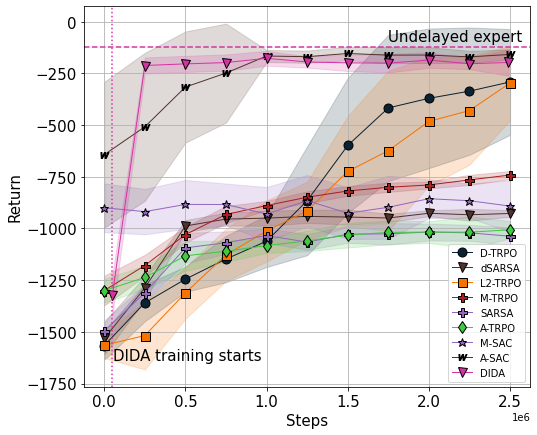
(a) Pendulum.

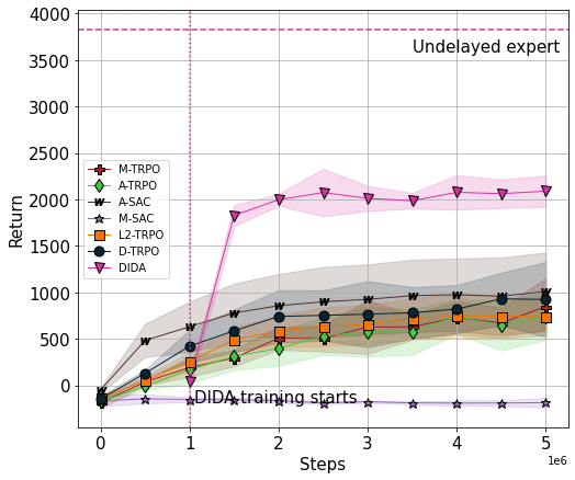
(b) HalfCheetah.

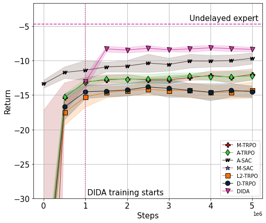
(c) Reacher.

Figure 1: For a 5-steps delay, mean return and one standard deviation (shaded) as a function of the number of steps sampled from the environment (10 seeds).

7 Experiments

7.1 Setting

As we have seen in the theoretical analysis, a smoother expert is beneficial for the performance bound of the imitated delayed policy. Therefore, in the following experiments, we consider expert policies learned with SAC. As reported in an extensive study about smooth policies (Mysore et al., 2021), the entropy-maximization framework of SAC is able to learn a smooth policy even without additional forms of regularization. To avoid ever-growing memory by storing all samples in the buffer as done in Algorithm 1, we use a maximum buffer size of 10 iterations for DIDA and overwrite the oldest iteration samples when this buffer is full. As suggested by Ross et al. (2011), we use $\beta_{1}=1,\beta_{i\geq 2}=0$ as mixture weights for the sampling policy. The policy for DIDA is a simple feed-forward neural network. More details and all hyper-parameters are reported in Section D.2.

We will test DIDA, along with some baselines from the state of the art, on the following environments.

Pendulum  The task of the agent is to rotate a pendulum upward. It is a classic experiment in delayed RL as delays are highly impacting performance due to unstable equilibrium in the upward position. We use the version from the library gym (Brockman et al., 2016).

Mujoco  Continuous robotic locomotion control tasks realized with an advanced physics simulator from the library mujoco (Todorov et al., 2012). Here the main difficulty lies in the complex dynamics and in the large state and action spaces. Among the possible environments, we consider the ones that are most affected by delays, namely Walker2d, HalfCheetah, Reacher, and Swimmer.

Trading  The agent trades the EUR-USD (€/$) currency pair on a minute-by-minute basis and can either buy, sell or stay flat against a fixed amount of USD, following the framework of Bisi et al. (2020) and Riva et al. (2021). We assume trading is without fees, but we do take the spread into account. To this setting, we add a delay of 10 seconds to the action execution. In this environment, we leverage the knowledge of an expert which is a policy trained on years 2016-2017 by Fitted Q-Iteration (FQI Ernst et al., 2005) with XGBoost (Chen & Guestrin, 2016) as a regressor for the $Q$ function. Only for this task, we use Extra Trees (Geurts et al., 2006) as policy for DIDA.

The baselines for comparison with our algorithm include a memoryless and an augmented version of TRPO (M-TRPO and A-TRPO respectively), D-TRPO and L2-TRPO (Liotet et al., 2021), SARSA (Sutton & Barto, 2018) and dSARSA (Schuitema et al., 2010). The last two algorithms involve state discretization and are thus tested on pendulum only. We consider also augmented SAC (A-SAC), considered also by Bouteiller et al. (2020), and memoryless SAC (M-SAC). Although SAC can be trained at every step as we do for Pendulum, we restrict training to every 50 steps on Mujoco to speed up the procedure and reduce memory usage. We have also considered adding DCAC (Bouteiller et al., 2020) but for computational reasons, we have decided not to include it. Early experimental results showed that its running time was more than 50 times the one of DIDA. For a fair comparison to the baselines, which learn a policy from scratch, we include the training steps of the expert in the step count of DIDA, as indicated by the vertical dotted line in the figures.

7.2 Results

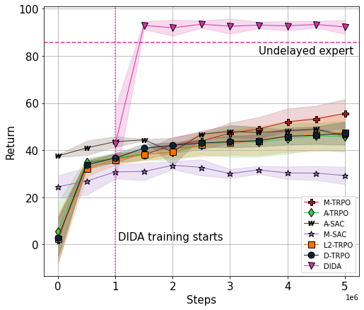
(a) Swimmer.

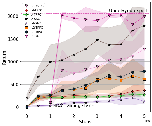
(b) Walker2d.

Figure 1: For a 5-steps delay, mean return and one standard deviation (shaded) as a function of the number of steps sampled from the environment (10 seeds).

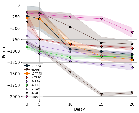
Figure 2: Mean return and its standard deviation (shaded) as a function delay (10 seeds).

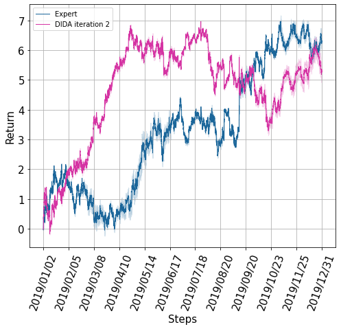
Figure 3: Evolution of the return of DIDA for the trading of the EUR-USD pair in 2019. Performance is computed in percentage w.r.t. the invested amount.

As we can see from the results on pendulum and mujoco, Figures 1(a), 1(b), 1(c), 2(a) and 2(b), DIDA is able to converge much faster than the baselines, in any environment with the exception of A-SAC on the pendulum environment. In less than half a million steps on mujoco, and 250.000 steps on pendulum, DIDA almost reaches its final performance. We note that, in HalfCheetah and Reacher, DIDA, although the best delayed algorithm, performs much worse than the expert. Surprisingly, in Swimmer, DIDA performs slightly better than the undelayed expert. All these phenomenons might actually be due to a single cause. In our implementation, to initialize the environment, a sequence of $\Delta-1$ random actions are applied in an undelayed environment to sample a first delayed augmented state. Depending on the environment, this sequence could cause the agent to start in un-advantageous or advantageous states. For instance, in HalfCheetah, the random action have put the agent head-down when the the latter is first allowed to control the environment. It must thus first get back on its feet before starting to move. On the contrary, in a simpler environment like Swimmer, the initial random action queue might give some initial speed to the agent, yielding higher rewards at the beginning than its undelayed counterpart.

We provide another experiment on Pendulum where we study the robustness of DIDA, as compared to baselines, against an increase in the delay for fixed hyper-parameters. We report the final mean return per episode for different values of the delay in Figure 2. Clearly, from all the baselines studied, DIDA is the most robust to the increase in the delay.

For the trading task, which is a batch-RL task since the training dataset is a fixed set of historical exchange rates, DIDA is prone to overfitting the expert policy on these examples. Therefore, after training several iterations of DIDA, we select the best iteration on the validation year 2018 and show the test performance in the year 2019 compared to the undelayed expert. In our results, we consider two experts trained on two different seeds, but with the same hyper-parameters configuration. We then imitated each seed with DIDA. The results, as shown in Figure 3, show the ability of DIDA to adapt to non-integer delays and maintain a positive return, which is not a simple task when taking the spread into account in trading the EUR-USD. One may notice that the delayed policy is able to outperform the expert on the first period of the test. This could be explained by the fact that the expert undelayed policy may have overfitted the training set while the imitation learning of an undelayed policy acted as a regularization. We provide an analysis on the policy learned by DIDA with respect to the expert in Section D.3.

Moreover, we provide in Section D.3 additional experiments on a stochastic version of pendulum and a study of the impact of a growing delay on the performance of DIDA.

8 Conclusion

In this paper, we explored the possibility of splitting delayed reinforcement learning into easier tasks, traditional undelayed reinforcement learning on the one hand, and imitation learning on the other one. We provided a theoretical analysis demonstrating bounds on the performance of a delayed policy compared to undelayed experts, both for integer or non-integer constant delays. These bounds apply in our particular setting but are also of interest in general for delayed policies. This guided us in the creation of our algorithm, DIDA, which learns a delayed policy by imitating an undelayed expert using DAgger. We have empirically shown that this idea, although rather simple, provides excellent results in practice, achieving high performance with remarkable sample efficiency and light computations. We believe that our work paves the way for many possible generalizations, which include stochastic delays and particular situations in which an undelayed simulator is not available, but where an undelayed dataset can be artificially created from delayed trajectories in order to train an expert offline.

Appendix A General Results

A.1 Bounds involving the Wasserstein distance

Proposition A.1.

Let X,Y be two random variables on $\mathbb{R}$ with distribution $\pi_{0},\pi_{1}$ respectively. Then,

$$\left|\operatorname*{\mathbb{E}}[X]-\operatorname*{\mathbb{E}}[Y]\right|\leq\mathcal{W}_{1}(\pi_{0}\|\pi_{1}).$$

Proof.

One has

$$\operatorname*{\mathbb{E}}[X]-\operatorname*{\mathbb{E}}[Y]=\int_{\mathbb{R}}x(\pi_{0}(x)-\pi_{1}(x))dx\leq\mathcal{W}_{1}(\pi_{0}\|\pi_{1}),$$

since $x\mapsto x$ is 1-LC. The same holds for $\operatorname*{\mathbb{E}}[Y]-\operatorname*{\mathbb{E}}[X]$, since the Wasserstein distance is symmetric. ∎

The next result asserts that if one applies a $L$-LC function to two random variables, one gets two random variables with distribution whose Wasserstein distance is bounded by the original Wasserstein distance multiplied by a factor $L$.

Proposition A.2.

Let $g:\Omega\rightarrow\mathbb{R}$ be an $L$-LC function and $\pi_{0},\pi_{1}$ two probability measures over the metric space $\Omega$. Note $g_{\pi}$ the distribution of the random variable $g(X)$ where $X$ is distributed according to $\pi$. Then,

$$\mathcal{W}_{1}(g_{\pi_{0}}\|g_{\pi_{1}})\leq L\mathcal{W}_{1}(\pi_{0}\|\pi_{1}).$$

Proof.

By definition of Wasserstein distance,

$$\mathcal{W}_{1}(g_{\pi_{0}}\|g_{\pi_{1}}) =\sup_{\left\|f\right\|_{L}\leq 1}\left|\int_{\mathbb{R}}f(x)(g_{\pi_{0}}(x)-g_{\pi_{1}}(x))dx\right|$$

$$=\sup_{\left\|f\right\|_{L}\leq 1}\left|\int_{\mathbb{R}}f(x)g_{\pi_{0}}(x)dx-\int_{\mathbb{R}}f(x)g_{\pi_{1}}(x)dx\right|.$$

We can then use the definitions of $g_{\pi_{0}}$ and $g_{\pi_{1}}$ to rewrite the previous formula in terms of expected values

$$\mathcal{W}_{1}(g_{\pi_{0}}\|g_{\pi_{1}}) =\sup_{\left\|f\right\|_{L}\leq 1}\left|\int_{\mathbb{R}}f(g(x))\pi_{0}(x)dx-\int_{\mathbb{R}}f(g(x))\pi_{1}(x)dx\right|$$

$$=\sup_{\left\|f\right\|_{L}\leq 1}\left|\int_{\mathbb{R}}f(g(x))(\pi_{0}(x)-\pi_{1}(x))dx\right|.$$

Since $g$ is $L_{g}$-LC by assumption, the composition $f(g(x))$ is still $L_{g}$-LC, so

$$\mathcal{W}_{1}(g_{\pi_{0}}\|g_{\pi_{1}}) \leq L_{g}\mathcal{W}_{1}(\pi_{0}\|\pi_{1}).$$

∎

Proposition A.3.

Consider an MDP with $\pi$ a policy such that its state-action value function is Lipschitz with constant $L_{Q}$ in the second argument, i.e. it satisfies, for all $s\in\mathcal{S}$ and $a,a^{\prime}\in\mathcal{A}$

$$\left|Q^{\pi}(s,a)-Q^{\pi}(s,a^{\prime})\right|\leq L_{Q}\operatorname{\text{d}}_{\mathcal{A}}(a,a^{\prime}),$$

then, for every couple of probability distributions $\eta,\nu$ over $\mathcal{A}$, one has that

$$\left|\operatorname*{\mathbb{E}}_{\begin{subarray}{c}X\sim\eta\\ Y\sim\nu\end{subarray}}[Q^{\pi}(s,X)-Q^{\pi}(s,Y)]\right|\leq L_{Q}\mathcal{W}_{1}(\eta(\cdot)\|\nu(\cdot)).$$

Proof.

We note $g_{\eta}$ and $g_{\nu}$ the respective distributions of $Q^{\pi}(s,X)$ and $Q^{\pi}(s,Y)$. First of all, we can apply A.1 to say that

$$\left|\operatorname*{\mathbb{E}}_{\begin{subarray}{c}X\sim\eta\\ Y\sim\nu\end{subarray}}[Q^{\pi}(s,X)-Q^{\pi}(s,Y)]\right|\leq\mathcal{W}_{1}(g_{\eta}\|g_{\nu}).$$

For a fixed $s\in\mathcal{S}$, the two random variables $Q^{\pi}(s,X)$ and $Q^{\pi}(s,Y)$ can be seen as the application of the $L_{Q}$-Lipschitz function $Q^{\pi}(s,\cdot):\ \mathcal{A}\to\mathbb{R}$ to $X$ and $Y$, respectively. This satisfies the assumptions of A.2, therefore

$$\mathcal{W}_{1}(Q^{\pi}(s,\eta(\cdot))\|Q^{\pi}(s,\nu(\cdot)))\leq L_{Q}\mathcal{W}_{1}(\eta(\cdot)\|\nu(\cdot)).$$

∎

Proposition A.4.

Consider an $L_{P}$ transition function $p$ and an $L_{\pi}$ policy $\pi$ in some MDP $\mathcal{M}$. Then, for any $f:~{}S\to~{}\mathbb{R}$ which is $1$-LC, we have that the function $g:~{}S\to~{}\mathbb{R}$ given by

$$g(s)\coloneqq\int_{\mathcal{S}}f(s^{\prime})\int_{A}p(s^{\prime}|s,a)\pi(a|s)~{}da~{}ds^{\prime}$$

is Lipschitz with constant $L_{p}(1+L_{\pi})$

Proof.

Let $s,z\in S$, one has

$$\lvert g(s)-g(z)\rvert =\left|\int_{\mathcal{S}}f(s^{\prime})\int_{A}p(s^{\prime}|s,a)\pi(a|s)-p(s^{\prime}|z,a)\pi(a|z)~{}da~{}ds^{\prime}\right|$$

$$\leq\left|\int_{\mathcal{S}}f(s^{\prime})\int_{A}p(s^{\prime}|s,a)\left(\pi(a|s)-\pi(a|z)\right)~{}da~{}ds^{\prime}\right|$$

$$\quad+\left|\int_{\mathcal{S}}f(s^{\prime})\int_{A}\left(p(s^{\prime}|s,a)-p(s^{\prime}|z,a)\right)\pi(a|z)~{}da~{}ds^{\prime}\right|$$ (5)

$$\leq\underbrace{\left|\int_{A}\left(\pi(a|s)-\pi(a|z)\right)\int_{\mathcal{S}}f(s^{\prime})p(s^{\prime}|s,a)~{}ds^{\prime}~{}da\right|}_{A}$$

$$\quad+\underbrace{\left|\int_{A}\pi(a|z)\int_{\mathcal{S}}f(s^{\prime})\left(p(s^{\prime}|s,a)-p(s^{\prime}|z,a)\right)~{}ds^{\prime}~{}da\right|}_{B},$$ (6)

where we add and remove the quantity $p(s^{\prime}|s,a)\pi(a|z)$ in Equation 5 and use Fubini’s theorem in Equation 6.

By Lipschitzness of $p$, we have that $a\mapsto\int_{\mathcal{S}}f(s^{\prime})p(s^{\prime}|s,a)~{}ds^{\prime}$ is $L_{p}$-LC. Thus,

$$A =L_{P}\left|\int_{A}\left(\pi(a|s)-\pi(a|z)\right)\frac{\int_{\mathcal{S}}f(s^{\prime})p(s^{\prime}|s,a)~{}ds^{\prime}}{L_{P}}~{}da\right|$$

$$\leq L_{\pi}L_{P}\operatorname{\text{d}}_{\mathcal{S}}(s,z)$$

For the second term, again, by Lipschitzness of $p$, we have

$$B \leq\left|\int_{A}L_{P}d_{\mathcal{S}}(s,z)\pi(a|z)~{}da\right|$$

$$=L_{P}d_{\mathcal{S}}(s,z).$$

Overall,

$$\lvert g(s)-g(z)\rvert \leq L_{p}(L_{\pi}+1)\operatorname{\text{d}}_{\mathcal{S}}(s,z).$$

∎

A.2 Bounding $\sigma_{b}^{\rho}$

We provide two bounds for $\sigma_{b}^{\rho}=\operatorname*{\mathbb{E}}_{\begin{subarray}{c}x^{\prime}\sim d^{\widetilde{\pi}}_{\rho}\\ s,s^{\prime}\sim b(\cdot|x^{\prime})\end{subarray}}\left[\operatorname{\text{d}}_{\mathcal{S}}(s,s^{\prime})\right]$ with $\rho$ a distribution on $\mathcal{S}$. The first uses the assumption that the state space in is $\mathbb{R}^{n}$ and is equipped with the Euclidean norm while the second assumes that the MDP is TLC.

Lemma A.1 (Euclidean bound).

Consider an MDP such that $\mathcal{S}\subset\mathbb{R}^{n}$ is equipped with the Euclidean norm. Then one has

$$\sigma_{b}^{\rho}\leq\operatorname*{\mathbb{E}}_{x^{\prime}\sim d_{\rho}^{\tilde{\pi}}(\cdot)}\left[\sqrt{\operatorname*{\mathbb{V}\mathrm{ar}}_{s\sim b(\cdot|x^{\prime})}(s|x^{\prime})}\right].$$

Proof.

We derive the following results which intermediate steps are detailed after.

$$\sigma_{b}^{\rho} =\operatorname*{\mathbb{E}}_{\begin{subarray}{c}x^{\prime}\sim d^{\widetilde{\pi}}_{\rho}\\ s,s^{\prime}\sim b(\cdot|x^{\prime})\end{subarray}}\left[\operatorname{\text{d}}_{\mathcal{S}}(s,s^{\prime})\right]$$

$$=\operatorname*{\mathbb{E}}_{\begin{subarray}{c}x^{\prime}\sim d^{\widetilde{\pi}}_{\rho}\\ s,s^{\prime}\sim b(\cdot|x^{\prime})\end{subarray}}\left[\sqrt{(s^{\prime}-s)^{2}}\right]$$ (7)

$$=\operatorname*{\mathbb{E}}_{x^{\prime}\sim d^{\widetilde{\pi}}_{\rho}}\sqrt{\operatorname*{\mathbb{E}}_{s,s^{\prime}\sim b(\cdot|x^{\prime})}\left[(s^{\prime}-s)^{2}\right]}.$$ (8)

Equation 7 follows from the definition of the Euclidean norm and Equation 8 is obtained by applying Jensen’s inequality. To conclude, since $s^{\prime}$ and $s$ are i.i.d., one has that $\operatorname*{\mathbb{E}}_{s,s^{\prime}\sim b(\cdot|x^{\prime})}\left[(s^{\prime}-s)^{2}\right]=2\mathbb{V}ar_{s\sim b(\cdot|x^{\prime})}[s]$. ∎

The following proposition is involved in the proof of the bound of $\sigma_{b}^{\rho}$ when the MDP is TLC.

Proposition A.5.

Consider an $L_{T}$-TLC MDP. Consider any augmented state $x=(s_{1},a_{1},\dots,a_{\Delta})\in\mathcal{S}\times\mathcal{A}^{\Delta}$ for a given $\Delta\in\mathbb{N}$. Then

$$\mathcal{W}_{1}\left(b(\cdot|x)\|\delta_{s_{1}}\right)\leq\Delta L_{T}$$

Proof.

We proceed by induction. The case case d=0 is true since the current state is known exactly without delay. The case d=1 is true by the assumption of $L_{T}$-TLC. Assume that the statement is true for $d\in\mathbb{N}$, then

$$\mathcal{W}_{1}\left(b(\cdot|x)\|\delta_{s_{1}}\right) =\sup_{\left\|f\right\|_{L}\leq 1}\left|\int_{\mathcal{S}}f(s^{\prime})\left(b(s^{\prime}|x)-\delta_{s_{1}}(s^{\prime})\right)ds^{\prime}\right|$$

$$=\sup_{\left\|f\right\|_{L}\leq 1}\left|\int_{\mathcal{S}}p(s_{2}|s_{1},a_{1})\int_{\mathcal{S}}f(s^{\prime})\left(b(s^{\prime}|s_{2},a_{2},\cdots,a_{\Delta})-\delta_{s_{1}}(s^{\prime})\right)ds^{\prime}\right|$$ (9)

$$=\sup_{\left\|f\right\|_{L}\leq 1}\left|\int_{\mathcal{S}}p(s_{2}|s_{1},a_{1})\int_{\mathcal{S}}f(s^{\prime})\left(b(s^{\prime}|s_{2},a_{2},\cdots,a_{\Delta})-\delta_{s_{2}}(s^{\prime})\right)ds^{\prime}\right.$$

$$\quad+\left.\int_{\mathcal{S}}p(s_{2}|s_{1},a_{1})\int_{\mathcal{S}}f(s^{\prime})\left(\delta_{s_{2}}(s)-\delta_{s_{1}}(s^{\prime})\right)ds^{\prime}\right|$$ (10)

$$\leq\underbrace{\sup_{\left\|f\right\|_{L}\leq 1}\left|\int_{\mathcal{S}}p(s_{2}|s_{1},a_{1})\int_{\mathcal{S}}f(s^{\prime})\left(b(s^{\prime}|s_{2},a_{2},\cdots,a_{\Delta})-\delta_{s_{2}}(s^{\prime})\right)ds^{\prime}\right|}_{A}$$

$$\quad+\underbrace{\mathcal{W}_{1}\left(P(|s_{1},a_{1})\|\delta_{s_{1}}\right)}_{B},$$

where (9) hols by conditioning on the second visited state $s_{2}$ and Equation 10 holds by adding and subtracting $\delta_{s_{2}}$. The reader may have recognized that the statement at $\Delta-1$ can be used to bound $A$ while $B$ can be bounded with the $L_{T}$-TLC assumption. Therefore

$$\mathcal{W}_{1}\left(b(\cdot|x)\|\delta_{s_{1}}\right)\leq dL_{T},$$

and the statement holds for any $\Delta\in\mathbb{N}$. ∎

Lemma A.2 (Time-Lipschitz bound).

Consider an $L_{T}$-Lipschitz MDP with delay $\Delta$. Then, one has

$$\sigma_{b}^{\rho}\leq 2\Delta L_{T}$$

Proof.

Call $s_{x}$ the state contained in $x$. By triangular inequality, one has

$$\sigma_{b}^{\rho} =\operatorname*{\mathbb{E}}_{\begin{subarray}{c}x\sim d^{\widetilde{\pi}}_{\rho}\\ s,s^{\prime}\sim b(\cdot|x)\end{subarray}}\left[\operatorname{\text{d}}_{\mathcal{S}}(s,s^{\prime})\right]$$

$$\leq\operatorname*{\mathbb{E}}_{\begin{subarray}{c}x\sim d^{\widetilde{\pi}}_{\rho}\\ s\sim b(\cdot|x^{\prime})\end{subarray}}\left[\operatorname{\text{d}}_{\mathcal{S}}(s,s_{x})\right]+\operatorname*{\mathbb{E}}_{\begin{subarray}{c}x\sim d^{\widetilde{\pi}}_{\rho}\\ s^{\prime}\sim b(\cdot|x)\end{subarray}}\left[\operatorname{\text{d}}_{\mathcal{S}}(s_{x},s^{\prime})\right]$$

$$=2\operatorname*{\mathbb{E}}_{x\sim d^{\widetilde{\pi}}_{\rho}}\left[\int_{\mathcal{S}}d_{\mathcal{S}}(s,s_{x})b(s|x)~{}ds\right]$$

$$=2\operatorname*{\mathbb{E}}_{x\sim d^{\widetilde{\pi}}_{\rho}}\left[\int_{\mathcal{S}}\operatorname{\text{d}}_{\mathcal{S}}(s,s_{x})\left(b(s|x)-\delta_{s_{x}}(s)\right)~{}ds\right]$$ (11)

$$\leq 2\operatorname*{\mathbb{E}}_{x\sim d^{\widetilde{\pi}}_{\rho}}\left[\mathcal{W}_{1}\left(b(\cdot|x)\|\delta_{s_{x}}\right)\right],$$ (12)

where Equation 11 holds because $\int_{\mathcal{S}}d_{\mathcal{S}}(s,s_{x})\delta_{s_{x}}(s)ds=0$ and Equation 12 follows by recognizing the Wasserstein distance. One can then use A.5 on each of the two terms to conclude. ∎

Appendix B Bounding the Value Function via Performance Difference Lemma

See 6.1

Proof.

We first prove the result for integer delay $d\in\mathbb{N}$. We start by adding and subtracting $\operatorname*{\mathbb{E}}_{\begin{subarray}{c}s\sim b(\cdot|x^{\prime})\\ a\sim\widetilde{\pi}(\cdot|x^{\prime})\end{subarray}}\left[r(s,a)+\gamma\operatorname*{\mathbb{E}}_{s^{\prime}\sim p(\cdot|s,a)}[V^{\pi_{E}}(s^{\prime})]\right]$ to the quantity of interest $I(x)=\operatorname*{\mathbb{E}}_{s\sim b(\cdot|x)}[V^{\pi_{E}}(s)]-V^{\widetilde{\pi}}(x)$.

This yields:

$$I(x) =\underbrace{\operatorname*{\mathbb{E}}_{s\sim b(\cdot|x)}[V^{\pi_{E}}(s)]-\operatorname*{\mathbb{E}}_{\begin{subarray}{c}s\sim b(\cdot|x^{\prime})\\ a\sim\widetilde{\pi}(\cdot|x^{\prime})\end{subarray}}\left[r(s,a)+\gamma\operatorname*{\mathbb{E}}_{s^{\prime}\sim p(\cdot|s,a)}[V^{\pi_{E}}(s^{\prime})]\right]}_{A}$$

$$\quad+\underbrace{\operatorname*{\mathbb{E}}_{\begin{subarray}{c}s\sim b(\cdot|x^{\prime})\\ a\sim\widetilde{\pi}(\cdot|x^{\prime})\end{subarray}}\left[r(s,a)+\gamma\operatorname*{\mathbb{E}}_{s^{\prime}\sim p(\cdot|s,a)}[V^{\pi_{E}}(s^{\prime})]\right]-V^{\widetilde{\pi}}(x)}_{B}.$$

The first term is

$$A=\operatorname*{\mathbb{E}}_{s\sim b(\cdot|x)}[V^{\pi_{E}}(s)]-\operatorname*{\mathbb{E}}_{\begin{subarray}{c}s\sim b(\cdot|x^{\prime})\\ a\sim\widetilde{\pi}(\cdot|x^{\prime})\end{subarray}}\left[Q^{\pi_{E}}(s,a)\right].$$

For the second term, note that $V^{\widetilde{\pi}}(x)=\operatorname*{\mathbb{E}}_{\begin{subarray}{c}s\sim b(\cdot|x^{\prime})\\ a\sim\widetilde{\pi}(\cdot|x^{\prime})\end{subarray}}\left[r(s,a)\right]+\gamma\operatorname*{\mathbb{E}}_{\begin{subarray}{c}x^{\prime}\sim\widetilde{p}(\cdot|x,a)\\ a\sim\widetilde{\pi}(\cdot|x^{\prime})\end{subarray}}[V^{\widetilde{\pi}}(x^{\prime})]$. Therefore,

$$B =\gamma\operatorname*{\mathbb{E}}_{\begin{subarray}{c}s\sim b(\cdot|x^{\prime})\\ a\sim\widetilde{\pi}(\cdot|x^{\prime})\end{subarray}}\left[\operatorname*{\mathbb{E}}_{s^{\prime}\sim p(\cdot|s,a)}[V^{\pi_{E}}(s^{\prime})]\right]-\gamma\operatorname*{\mathbb{E}}_{\begin{subarray}{c}x^{\prime}\sim\widetilde{p}(\cdot|x,a)\\ a\sim\widetilde{\pi}(\cdot|x^{\prime})\end{subarray}}[V^{\widetilde{\pi}}(x^{\prime})].$$

By observing that $\int_{\mathcal{S}}b(s|x)p(s^{\prime}|s,a)ds=\int_{\mathcal{X}}\tilde{p}(x^{\prime}|x,a)b(s^{\prime}|x^{\prime})dx^{\prime}$, that is, compute the current state with the belief then the next current state is equivalent to computing the next extended state and then the next current state with the belief. Thus,

$$B =\gamma\operatorname*{\mathbb{E}}_{\begin{subarray}{c}x^{\prime}\sim\widetilde{p}(\cdot|x,a)\\ a\sim\widetilde{\pi}(\cdot|x^{\prime})\end{subarray}}\left[\operatorname*{\mathbb{E}}_{s\sim b(\cdot|x^{\prime})}[V^{\pi_{E}}(s^{\prime})]-V^{\widetilde{\pi}}(x^{\prime})\right]$$

$$=\gamma\operatorname*{\mathbb{E}}_{\begin{subarray}{c}x^{\prime}\sim\widetilde{p}(\cdot|x,a)\\ a\sim\widetilde{\pi}(\cdot|x^{\prime})\end{subarray}}\left[I(x^{\prime})\right],$$

where we have recognised the quantity of interest $I$ taken at another extended state. One can thus iterate as in the original performance difference lemma to get

$$I(x) =\sum_{t=0}^{\infty}\gamma^{t}\mathbb{E}^{\widetilde{\pi}}\left[\left.\operatorname*{\mathbb{E}}_{s\sim b(\cdot|x_{t})}[V^{\pi_{E}}(s)]-\operatorname*{\mathbb{E}}_{\begin{subarray}{c}s\sim b(\cdot|x_{t})\\ a\sim\widetilde{\pi}(\cdot|x_{t})\end{subarray}}[Q^{\pi_{E}}(s,a)]\right|x_{0}=x\right]$$

$$=\frac{1}{1-\gamma}\operatorname*{\mathbb{E}}_{x^{\prime}\sim d^{\widetilde{\pi}}_{x}}\left[\operatorname*{\mathbb{E}}_{s\sim b(\cdot|x^{\prime})}[V^{\pi_{E}}(s)]-\operatorname*{\mathbb{E}}_{\begin{subarray}{c}s\sim b(\cdot|x^{\prime})\\ a\sim\widetilde{\pi}(\cdot|x^{\prime})\end{subarray}}[Q^{\pi_{E}}(s,a)]\right],$$ (13)

where Equation 13 is obtained by recognising the discounted state distribution under policy $\widetilde{\pi}$. This completes the proof.

We now assume non-integer delay, setting $\Delta\in(0,1)$ but the proof for $\Delta\in\mathbb{R}$ follows easily. The proof is the same as above except for substituting $b$ with $b_{\Delta}$. One step which might not be evident is that

$$\int_{\mathcal{S}}b_{\Delta}(s_{t+\Delta}|x_{t})p(s_{t+1+\Delta}|s_{t+\Delta},a)~{}ds_{t+\Delta}=\int_{\mathcal{X}}\tilde{p}(x_{t+1}|x_{t},a)b_{\Delta}(s_{t+1+\Delta}|x_{t+1})~{}dx_{t+1}.$$

This is true because, for $x_{t}=(s_{t},a_{t-1}),x_{t+1}=(s_{t+1},a_{t})\in\mathcal{X}$,

$$\int_{\mathcal{S}}b_{\Delta}(s_{t+\Delta}|x_{t}) p(s_{t+1+\Delta}|s_{t+\Delta},a)~{}ds_{t+\Delta}$$

$$=\int_{\mathcal{S}}b_{\Delta}(s_{t+\Delta}|x_{t})\int_{\mathcal{S}}b_{\Delta}(s_{t+1+\Delta}|s_{t+1},a)b_{1-\Delta}(s_{t+1}|s_{t+\Delta},a)~{}ds_{t+1}~{}ds_{t+\Delta}$$ (14)

$$=\int_{\mathcal{S}}b_{\Delta}(s_{t+1+\Delta}|s_{t+1},a)\int_{\mathcal{S}}b_{\Delta}(s_{t+\Delta}|x_{t})b_{1-\Delta}(s_{t+1}|s_{t+\Delta},a)~{}ds_{t+\Delta}~{}ds_{t+1}$$

$$=\int_{\mathcal{S}}b_{\Delta}(s_{t+1+\Delta}|s_{t+1},a)\int_{\mathcal{S}}b_{\Delta}(s_{t+\Delta}|s_{t},a_{t-1})b_{1-\Delta}(s_{t+1}|s_{t+\Delta},a)~{}ds_{t+\Delta}~{}ds_{t+1}$$

$$=\int_{\mathcal{A}}\int_{\mathcal{S}}b_{\Delta}(s_{t+1+\Delta}|s_{t+1},a_{t})\delta_{a}(a_{t})\int_{\mathcal{S}}b_{\Delta}(s_{t+\Delta}|s_{t},a_{t-1})b_{1-\Delta}(s_{t+1}|s_{t+\Delta},a)~{}ds_{t+\Delta}~{}ds_{t+1}~{}da_{t}$$ (15)

$$=\int_{\mathcal{X}}b_{\Delta}(s_{t+1+\Delta}|x_{t+1})\tilde{p}(x_{t+1}|x_{t},a)~{}dx_{t+1}$$

where Equation 14 holds by replacing the transition $p$ as in Equation 4 and Equation 15 holds by definition of the transition in the augmented MDP. ∎

See 6.1

Proof.

We first prove the result for integer delay $\Delta\in\mathbb{N}$. The first step in this proof is to use the results of 6.1, which yields, for any $x\in\mathcal{X}$:

$$\operatorname*{\mathbb{E}}_{s\sim b(\cdot|x)} [V^{\pi_{E}}(s)]-V^{\widetilde{\pi}_{b}}(x)\leq\frac{1}{1-\gamma}\operatorname*{\mathbb{E}}_{x^{\prime}\sim d^{\widetilde{\pi}_{b}}_{x}}\left[\underbrace{\operatorname*{\mathbb{E}}_{s\sim b(\cdot|x^{\prime})}[V^{\pi_{E}}(s)]-\operatorname*{\mathbb{E}}_{\begin{subarray}{c}s\sim b(\cdot|x^{\prime})\\ a\sim\widetilde{\pi}_{b}(\cdot|x^{\prime})\end{subarray}}[Q^{\pi_{E}}(s,a)]}_{A}\right].$$

We consider the term inside the expectation over $x^{\prime}$, called $A$. We reformulate this term to highlight how we then apply A.3.

$$A =\operatorname*{\mathbb{E}}_{s\sim b(\cdot|x^{\prime})}\left[\operatorname*{\mathbb{E}}_{\begin{subarray}{c}a_{1}\sim\pi_{E}(\cdot|s)\\ a_{2}\sim\widetilde{\pi}_{b}(\cdot|x^{\prime})\end{subarray}}\left[Q^{\pi_{E}}(s,a_{1})-Q^{\pi_{E}}(s,a_{2})\right]\right]$$

$$\leq L_{Q}\operatorname*{\mathbb{E}}_{s\sim b(\cdot|x^{\prime})}\left[\mathcal{W}_{1}(\pi_{E}(\cdot|s)\|\widetilde{\pi}_{b}(\cdot|x^{\prime}))\right].$$ (16)

To finish the proof, it remains to bound below $\sigma_{b}^{x}\coloneq\operatorname*{\mathbb{E}}_{\begin{subarray}{c}x^{\prime}\sim d^{\widetilde{\pi}_{b}}_{x}\\ s,s^{\prime}\sim b(\cdot|x^{\prime})\end{subarray}}\left[\operatorname{\text{d}}_{\mathcal{S}}(s,s^{\prime})\right]$ with $\operatorname*{\mathbb{E}}_{s\sim b(\cdot|x^{\prime})}\left[\mathcal{W}_{1}(\pi_{E}(\cdot|s)\|\widetilde{\pi}_{b}(\cdot|x^{\prime}))\right]$.

One has

$$\mathcal{W}_{1}(\pi_{E}(\cdot|s)\|\widetilde{\pi}_{b}(\cdot|x^{\prime})) =\sup_{\left\|f\right\|_{L}\leq 1}\left|\int_{\mathcal{A}}f(a)(\pi_{E}(a|s)-\widetilde{\pi}_{b}(a|x^{\prime}))da\right|$$

$$=\sup_{\left\|f\right\|_{L}\leq 1}\left|\int_{\mathcal{A}}f(a)(\pi_{E}(a|s)-\int_{\mathcal{S}}\pi_{E}(a|s^{\prime})b(s^{\prime}|x^{\prime})ds^{\prime})da\right|$$ (17)

$$\leq\int_{\mathcal{S}}b(s^{\prime}|x^{\prime})\sup_{\left\|f\right\|_{L}\leq 1}\left|\int_{\mathcal{A}}f(a)(\pi_{E}(a|s)-\pi_{E}(a|s^{\prime}))da\right|ds^{\prime}$$ (18)

$$\leq\int_{\mathcal{S}}b(s^{\prime}|x^{\prime})\mathcal{W}_{1}(\pi_{E}(\cdot|s)\|\pi_{E}(\cdot|s^{\prime}))ds^{\prime}$$

$$\leq L_{\pi}\int_{\mathcal{S}}b(s^{\prime}|x^{\prime})\operatorname{\text{d}}_{\mathcal{S}}(s,s^{\prime})ds^{\prime},$$ (19)

where Equation 17 holds by definition of the optimal imitated delayed policy (see Equation 3), Equation 18 holds by application of Fubini-Tonelli’s theorem and Equation 19 holds by Lipschitzness of the expert undelayed policy. By re-injecting this result into Equation 16 we get the desired result.

We now assume non-integer delay, setting $\Delta\in(0,1)$ but the proof for $\Delta\in\mathbb{R}$ follows easily. In this case, the optimal policy learnt by DIDA is

$$\widetilde{\pi}_{b}(a|x)=\int_{\mathcal{S}}b_{\Delta}(s|x)\pi_{E}(a|s)ds..$$ (20)

The proof remains the same except for the first step, where the performance difference lemma is of course replaced by its non-integer delay version just discussed. ∎

See 6.2

Proof.

The result follows from application of A.1 to 6.1. ∎

See 6.1

Proof.

The result follows from application of A.2 to 6.1. ∎

B.1 Lower Bounding the Value Function

See 6.2

Proof.

We consider an MDP $\mathcal{M}=(\mathcal{S},\mathcal{A},p,R,\mu,\gamma)$ such that $\mathcal{S}=\mathbb{R}$ and $\mathcal{A}=\mathbb{R}$, its state transition is given by $s_{t+1}=s_{t}+\frac{a}{L_{\pi}}+\varepsilon_{t}$, where $\varepsilon_{t}\overset{i.i.d.}{\sim}\mathcal{N}(0,\sigma^{2})$. The transition distribution can be written as

$$p(s^{\prime}|s,a)=\mathcal{N}\left(s^{\prime};\ s+\frac{a}{L_{\pi}},\sigma^{2}\right).$$

Defining $L_{r}:=L_{Q}L_{\pi}$, the reward is given by $r(s,a)=-L_{r}\left|s+\frac{a}{L_{\pi}}\right|$. Note that the reward is always negative, yet the policy $\pi^{*}(\cdot|s)=\delta_{-L_{\pi}s}(s^{\prime})$ always yields $0$ reward and is therefore optimal. Clearly, its value function satisfies $V^{*}(s)=0$ for every $s\in\mathcal{S}$. Its $Q$ function is

$$Q^{*}(s,a) =-L_{r}\left|s+\frac{a}{L_{\pi}}\right|+\gamma\int_{\mathbb{R}}V^{*}(s^{\prime})\ p(s^{\prime}|s,a)\ ds^{\prime}$$

$$=-L_{r}\left|s+\frac{a}{L_{\pi}}\right|$$

$$=-L_{Q}\left|L_{\pi}s+a\right|.$$

Therefore, $Q^{*}$ is indeed $L_{Q}$-LC in the second argument.

Consider now any $\Delta$-delayed policy $\widetilde{\pi}$. At each time step $t$, the current state $s_{t}$ can be decomposed in this way

$$s_{t}=\underbrace{s_{t-\Delta-1}+\sum_{\tau=t-\Delta-1}^{t-1}\frac{a_{\tau}}{L_{\pi}}}_{\eqqcolon\phi(x_{t})}+\underbrace{\sum_{\tau=t-\Delta-1}^{t-1}\varepsilon_{\tau}}_{\epsilon},$$

where the first quantity is a deterministic function of the extended state, while the second is distributed under $\mathcal{N}(0,d\sigma^{2})$. The expected value of the instantaneous reward is then given by

$$\operatorname*{\mathbb{E}}[r(x_{t},a)] =-L_{r}\operatorname*{\mathbb{E}}\left[\left|s_{t}+\frac{a}{L_{\pi}}\right|\right]$$

$$=-L_{r}\operatorname*{\mathbb{E}}\left[\left|\phi(x_{t})+\frac{a}{L_{\pi}}+\sum_{\tau=t-\Delta-1}^{t-1}\varepsilon_{\tau}\right|\right].$$

The function $f:y\mapsto\operatorname*{\mathbb{E}}\left[\left|\mathcal{N}(y,\sigma)\right|\right]$ has minimum at 0 by symmetry of the normal distribution. Its value is the mean of a half-normal distribution, that is $\operatorname*{\mathbb{E}}\left[\left|\mathcal{N}(0,\sigma)\right|\right]=\frac{\sqrt{2}}{\sqrt{\pi}}\sigma$. Therefore

$$\operatorname*{\mathbb{E}}[r(x_{t},a)] \leq-L_{r}\frac{\sqrt{2}}{\sqrt{\pi}}\sqrt{d}\sigma,$$

which implies

$$V^{\widetilde{\pi}}(x_{t}) \leq-\frac{L_{r}}{1-\gamma}\frac{\sqrt{2}}{\sqrt{\pi}}\sqrt{d}\sigma$$

$$=-\frac{L_{Q}L_{\pi}}{1-\gamma}\frac{\sqrt{2}}{\sqrt{\pi}}\sqrt{\operatorname*{\mathbb{V}\mathrm{ar}}_{s\sim b(\cdot|x^{\prime})}(s|x^{\prime})},$$

by noticing that $L_{r}=L_{Q}L_{\pi}$ and that $\mathbb{V}ar_{s\sim b(\cdot|x)}(s|x)=d\sigma^{2}$. Note that $\sqrt{\operatorname*{\mathbb{V}\mathrm{ar}}_{s\sim b(\cdot|x)}(s|x)}$ is the same for each $x\in\mathcal{X}$ so we can replace it with $\operatorname*{\mathbb{E}}_{x^{\prime}\sim d_{x}^{\tilde{\pi}}(\cdot)}\left[\sqrt{\operatorname*{\mathbb{V}\mathrm{ar}}_{s\sim b(\cdot|x^{\prime})}(s|x^{\prime})}\right]$ to have a result more similar to 6.1.

Recalling that the optimal value function had value 0 at any state concludes the proof. ∎

Appendix C Bounding the Value Function via the State Distribution

For this bound, we wish to use the difference in state distribution between the delayed and the undelayed expert to grasp their difference. Obviously, they do not share the same state space since the DMDP is handled by augmenting the state. However, it is possible to define a unifying framework with the following object. In this section, we consider $\Delta\in\mathbb{N}$.

Definition C.1 ($\Delta^{\text{th}}$-order MDP).

Given an MDP $\mathcal{M}=(\mathcal{S},\mathcal{A},p,R,\mu)$, we define its correspondent $\Delta^{\text{th}}$-order MDP, $\Delta\in\mathbb{N}$, as the MDP $\widebar{\mathcal{M}}$ (a “$\ \widebar{}\$” will be used to refer to an element of an $\Delta^{\text{th}}$-order MDP) with

• State space $\widebar{\mathcal{S}}=\mathcal{S}^{\Delta+1}\times\mathcal{A}^{\Delta}$, whose states $\widebar{s}$ are composed of the last $\Delta+1$ states and $\Delta$ actions of the MDP, namely $\widebar{s}=(s_{1},a_{1},s_{2},a_{2},\dots,s_{\Delta},a_{\Delta},s_{\Delta+1})$.

• Unchanged action space $\mathcal{A}$.

• Reward function $R$, overwriting the undelayed notation but using as input a $\Delta^{\text{th}}$-order state, such that
  $R(\widebar{s}_{t},a)=R(s_{t},a)$. The overwriting is justified by this equality.

• Transition function $\widebar{p}$ given by

  $$\widebar{p}(\widebar{s}^{\prime}|\widebar{s},a)=p(s_{\Delta+1}^{\prime}|s_{\Delta+1},a)\delta_{a}(a_{\Delta}^{\prime})\prod_{i=1}^{\Delta}\delta_{s_{i+1}}(s_{i}^{\prime})\prod_{i=1}^{d-1}\delta_{a_{i+1}}(a_{i}^{\prime}),$$ (21)

  where $\widebar{s}=(s_{1},a_{1},\dots,a_{\Delta},s_{\Delta+1})$ and $\widebar{s}^{\prime}=(s_{1}^{\prime},a_{1}^{\prime},\dots,a_{\Delta}^{\prime},s_{\Delta+1}^{\prime})$ .

• The initial state distribution $\widebar{\mu}$ is such that the inital action queue $x$ is distributed as in the delayed MDP while the states of the states queue are distributed as $s_{i+1}\sim p(\cdot|s_{i},a_{i})$.

This definition is inspired from the concept of $\Delta^{\text{th}}$-order Markov chain. In this definition, $s_{\Delta+1}$ is intended to be the current state, while $s_{1}$ is the $\Delta$-delayed state, $a_{1:\Delta}$ is the action queue. Therefore, from the state of the $\Delta^{\text{th}}$-order MDP, one can either extract an extended state and query a delayed policy or the extract the current state and query an undelayed policy. This implies that one can define the state distribution on the $\Delta^{\text{th}}$-order MDP for both an undelayed and a delayed policy. We overwrite the notations and write respectively $d^{\pi}$ and $d^{\widebar{\pi}}$ the distribution of state on the $\Delta^{\text{th}}$-order MDP. The fact that the distribution concerns a $\Delta^{\text{th}}$-order state and not a state from the underlying MDP or DMDP will be clear from the notation of the variable which is sampled from this distribution. For instance, in $s\sim d^{\pi}$, $d^{\pi}$ is a distribution defined by applying $\pi$ on the undelayed MDP while $\tilde{s}\sim d^{\pi}$ assumes a distribution under $\pi$ on the $\Delta^{\text{th}}$-order MDP.

Before deriving bounds on the $\Delta^{\text{th}}$-order state probability distribution, we first prove a Lipschitzness result concerning the $\Delta^{\text{th}}$-order MDP which be used in later proofs.

Lemma C.1.

Consider an $(L_{P},L_{r})$-LC MDP and its $\Delta^{\text{th}}$-order MDP counterpart. Let $f:\widebar{\mathcal{S}}\to\mathbb{R}$ such that $\lVert f\rVert_{L}\leq 1$ w.r.t. to the L2-norm on $\widebar{\mathcal{S}}$. Then, the function

$$g_{f}:\widebar{\mathcal{S}}\times\mathcal{A} \longrightarrow\mathbb{R}$$

$$(\widebar{s},a) \longmapsto\int_{\widebar{\mathcal{S}}}f(\widebar{s}^{\prime})\widebar{p}(\widebar{s}^{\prime}|\widebar{s},a)~{}d\widebar{s}^{\prime},$$

is $L_{P}$-LC w.r.t. the second variable.

Proof.

Let $\widebar{s}\in\widebar{\mathcal{S}}$ such that $\widebar{s}=(s_{1},a_{1},\dots,a_{\Delta},s_{\Delta+1})$ and $a,b\in\mathcal{A}$. Then,

$$\left|g_{f}(\widebar{s},a)-g_{f}(\widebar{s},b)\right| =\left|\int_{\widebar{\mathcal{S}}}f(\widebar{s}^{\prime})\left(\widebar{p}(\widebar{s}^{\prime}|\widebar{s},a)-\widebar{p}(\widebar{s}^{\prime}|\widebar{s},b)\right)~{}d\widebar{s}^{\prime}\right|$$

$$=\left|\int_{\mathcal{S}\times\mathcal{A}}f(s_{2},a_{2},\dots,s_{\Delta+1},a_{\Delta+1}^{\prime},s_{\Delta+1}^{\prime})\right.$$ (22)

$$\quad\left.\vphantom{\int}\left({p}(s_{\Delta+1}^{\prime}|s_{\Delta+1},a)\delta_{a}(a_{\Delta+1}^{\prime})-{p}(s_{\Delta+1}^{\prime}|s_{\Delta+1},b)\delta_{b}(a_{\Delta+1}^{\prime})\right)~{}ds_{\Delta+1}^{\prime}~{}da_{\Delta+1}^{\prime}\right|$$ (23)

where in Equation 23 we integrate over the elements of $\widebar{s}$ fixed by the Dirac distributions of Equation 21 except for the last action. Note that $h\coloneqq(s,a)\mapsto f(s_{2},a_{2},\dots,s_{\Delta+1},a,s)$ is 1-LC because $f$ is 1-LC. We add and substract the quantity ${p}(s_{\Delta+1}^{\prime}|s_{\Delta+1},b)\delta_{a}(a_{\Delta+1})$ inside the integral to get

$$\left|g_{f}(\widebar{s},a)-g_{f}(\widebar{s},b)\right| \leq\left|\int_{\mathcal{S}\times\mathcal{A}}\delta_{a}(a_{\Delta+1}^{\prime})h(a_{\Delta+1}^{\prime},s_{\Delta+1}^{\prime})\left({p}(s_{\Delta+1}^{\prime}|s_{\Delta+1},a)-{p}(s_{\Delta+1}^{\prime}|s_{\Delta+1},b)\right)~{}ds_{\Delta+1}^{\prime}~{}da_{\Delta+1}^{\prime}\right|$$

$$\quad+\left|\int_{\mathcal{S}\times\mathcal{A}}h(a_{\Delta+1}^{\prime},s_{\Delta+1}^{\prime}){p}(s_{\Delta+1}^{\prime}|s_{\Delta+1},b)\left(\delta_{a}(a_{\Delta+1}^{\prime})-\delta_{b}(a_{\Delta+1}^{\prime})\right)~{}ds_{\Delta+1}^{\prime}~{}da_{\Delta+1}^{\prime}\right|$$

$$\leq(L_{P}+1)\operatorname{\text{d}}_{\mathcal{A}}(a,b),$$

where the last inequality follows by integrating over $s_{\Delta+1}^{\prime}$ for the first integral and $a_{\Delta+1}^{\prime}$ for the second, before taking the supremum over functions $h$ and recognising the Wasserstein distance. ∎

We can now prove a first important intermediary result which bounds the Wasserstein divergence in discounted state distribution in the $\Delta^{\text{th}}$-order MDP between the undelayed and the delayed policy.

Theorem C.1.

Consider an $(L_{P},L_{r})$-LC MDP $\mathcal{M}$ and its $(L_{\widebar{P}},L_{r})$-LC $\Delta^{\text{th}}$-order MDP counterpart $\widebar{\mathcal{M}}$. Let $\pi_{E}$ be a $L_{\pi}$-LC undelayed policy and assume that $\gamma L_{P}(1+L_{\pi})\leq 1$. Let $\widetilde{\pi}_{b}$ be a delayed policy as defined in Equation 3. Then, the two discounted state distributions $d_{\widebar{\mu}}^{\pi_{E}},d_{\widebar{\mu}}^{\widetilde{\pi}_{b}}$ defined on $\widebar{\mathcal{M}}$ satisfy

$$\mathcal{W}_{1}\left(d_{\widebar{\mu}}^{\pi_{E}}\|d_{\widebar{\mu}}^{\widetilde{\pi}_{b}}\right)\leq\gamma L_{Q}(1+L_{P})\sigma_{b}^{\widetilde{\mu}}$$

where $\sigma_{b}^{\widetilde{\mu}}=\operatorname*{\mathbb{E}}_{\begin{subarray}{c}x\sim d^{\widetilde{\pi}_{b}}_{\widetilde{\mu}}\\ s,s^{\prime}\sim b(\cdot|x)\end{subarray}}\left[\operatorname{\text{d}}_{\mathcal{S}}(s,s^{\prime})\right]$ and $d^{\widetilde{\pi}_{b}}_{\widetilde{\mu}}$ is defined on the DMDP.

Proof.

We start by developing the term $\mathcal{W}_{1}\left(d_{\widebar{\mu}}^{\pi_{E}}\|d_{\widebar{\mu}}^{\widetilde{\pi}_{b}}\right)$, using the supremum over the space of functions $f:\widebar{\mathcal{S}}\to\mathbb{R}$ such that $\lVert f\rVert_{L}\leq 1$ w.r.t. to the L2-norm on $\widebar{\mathcal{S}}$.

$$\mathcal{W}_{1}\left(d_{\widebar{\mu}}^{\pi_{E}}\|d_{\widebar{\mu}}^{\widetilde{\pi}_{b}}\right)=\sup_{\left\|f\right\|_{L}\leq 1}\left|\int_{\widebar{\mathcal{S}}}f(\widebar{s})\left(d_{\widebar{\mu}}^{\pi_{E}}(\widebar{s})-d_{\widebar{\mu}}^{\widetilde{\pi}_{b}}(\widebar{s})\right)~{}d\widebar{s}\right|.$$

We then use the fact that for some policy $\pi\in\Pi$, $d_{\widebar{\mu}}^{\pi}(\widebar{s})=(1-\gamma)\widebar{\mu}(\widebar{s})+\gamma\int_{\widebar{\mathcal{S}}}\widebar{p}^{\pi}(\widebar{s}|\widebar{s}^{\prime})d_{\widebar{\mu}}^{\pi}(\widebar{s}^{\prime})~{}d\widebar{s}^{\prime}$, where $\widebar{p}^{\pi}(\widebar{s}|\widebar{s}^{\prime})=\int_{\mathcal{A}}p(\widebar{s}^{\prime}|\widebar{s},a)\pi(a|\widebar{s})~{}da$ to yield

$$\mathcal{W}_{1}\left(d_{\widebar{\mu}}^{\pi_{E}}\|d_{\widebar{\mu}}^{\widetilde{\pi}_{b}}\right) =\gamma\sup_{\left\|f\right\|_{L}\leq 1}\left|\int_{\widebar{\mathcal{S}}}f(\widebar{s})\int_{\widebar{\mathcal{S}}}\left(\widebar{p}^{\pi_{E}}(\widebar{s}|\widebar{s}^{\prime})d_{\widebar{\mu}}^{\pi_{E}}(\widebar{s}^{\prime})-\widebar{p}^{\widetilde{\pi}_{b}}(\widebar{s}|\widebar{s}^{\prime})d_{\widebar{\mu}}^{\widetilde{\pi}_{b}}(\widebar{s}^{\prime})\right)~{}d\widebar{s}^{\prime}~{}d\widebar{s}\right|$$

$$\leq\gamma\underbrace{\sup_{\left\|f\right\|_{L}\leq 1}\left|\int_{\widebar{\mathcal{S}}}f(\widebar{s})\int_{\widebar{\mathcal{S}}}\left(d_{\widebar{\mu}}^{\pi_{E}}(\widebar{s}^{\prime})-d_{\widebar{\mu}}^{\widetilde{\pi}_{b}}(\widebar{s}^{\prime})\right)\widebar{p}^{\pi_{E}}(\widebar{s}|\widebar{s}^{\prime})~{}d\widebar{s}^{\prime}~{}d\widebar{s}\right|}_{A}$$

$$\quad+\gamma\underbrace{\sup_{\left\|f\right\|_{L}\leq 1}\left|\int_{\widebar{\mathcal{S}}}f(\widebar{s})\int_{\widebar{\mathcal{S}}}\left(\widebar{p}^{\pi_{E}}(\widebar{s}|\widebar{s}^{\prime})-\widebar{p}^{\widetilde{\pi}_{b}}(\widebar{s}|\widebar{s}^{\prime})\right)d_{\widebar{\mu}}^{\widetilde{\pi}_{b}}(\widebar{s}^{\prime})~{}d\widebar{s}^{\prime}~{}d\widebar{s}\right|}_{B},$$ (24)

where Equation 24 follows by adding and subtracting the term $\widebar{p}^{\pi_{E}}(\widebar{s}|\widebar{s}^{\prime})d_{\widebar{\mu}}^{\widetilde{\pi}_{b}}(\widebar{s}^{\prime})$ and using the triangular inequality.

The first term $A$ can be bounded by using Fubini’s theorem first and then leveraging A.4 which implies that $\int_{\widebar{\mathcal{S}}}f(\widebar{s})\widebar{p}^{\pi_{E}}(\widebar{s}|\widebar{s}^{\prime})~{}d\widebar{s}^{\prime}$ is $L_{P}(1+L_{\pi})$-LC. Therefore

$$A\leq L_{P}(1+L_{\pi})\mathcal{W}_{1}\left(d_{\widebar{\mu}}^{\pi_{E}}\|d_{\widebar{\mu}}^{\widetilde{\pi}_{b}}\right)$$

Now looking at the second term $B$, we will develop the term $\widebar{p}^{\pi_{E}}$ and $\widebar{p}^{\widetilde{\pi}_{b}}$ to highlight the influence of the policy and leverage Equation 3. We note $\widebar{s}=(s_{1},a_{1},\dots,a_{\Delta},s_{\Delta+1})$ and $\widebar{s}^{\prime}=(s_{1}^{\prime},a_{1}^{\prime},\dots,a_{\Delta}^{\prime},s_{\Delta+1}^{\prime})$. Moreover, we overwrite the notation of the belief to use it on a $\Delta^{\text{th}}$-order state such that $b(z|\widebar{s})=b(z|s_{1},a_{1},\dots,a_{\Delta})$, that is, the belief is based on the augmented state constructed from the oldest state inside $\widebar{s}$ and the sequence of action it contains.

$$B =\sup_{\left\|f\right\|_{L}\leq 1}\left|\int_{\widebar{\mathcal{S}}}f(\widebar{s})\int_{\widebar{\mathcal{S}}}\left(\int_{\mathcal{A}}\widebar{p}(\widebar{s}|\widebar{s}^{\prime},a)\pi_{E}(a|s_{\Delta+1}^{\prime})~{}da-\int_{\mathcal{A}}\int_{z\in\mathcal{S}}\widebar{p}(\widebar{s}|\widebar{s}^{\prime},a)b(z|\widebar{s}^{\prime})\pi_{E}(a|z)~{}dz~{}da\right)d_{\widebar{\mu}}^{\widetilde{\pi}_{b}}(\widebar{s}^{\prime})~{}d\widebar{s}^{\prime}~{}d\widebar{s}\right|$$

$$=\sup_{\left\|f\right\|_{L}\leq 1}\left|\int_{\widebar{\mathcal{S}}}f(\widebar{s})\left(\int_{\widebar{\mathcal{S}}}\int_{\mathcal{A}}\underbrace{\left(\pi_{E}(a|s_{\Delta+1}^{\prime})-\int_{z\in\mathcal{S}}b(z|\widebar{s}^{\prime})\pi_{E}(a|z)~{}dz\right)}_{C}\widebar{p}(\widebar{s}|\widebar{s}^{\prime},a)~{}da~{}d_{\widebar{\mu}}^{\widetilde{\pi}_{b}}(\widebar{s}^{\prime})~{}d\widebar{s}^{\prime}~{}d\widebar{s}\right)\right|,$$

where the term $C$ in this equation accounts for the difference in taking an action with the undelayed policy $\pi_{E}$ instead of the belief-based policy. Fubini’s theorem yields

$$B =\sup_{\left\|f\right\|_{L}\leq 1}\left|\int_{\widebar{\mathcal{S}}}\int_{\mathcal{A}}\left(\pi_{E}(a|s_{\Delta+1}^{\prime})-\int_{z\in\mathcal{S}}b(z|\widebar{s}^{\prime})\pi_{E}(a|z)~{}dz\right)\underbrace{\left(\int_{\widebar{\mathcal{S}}}f(\widebar{s})\widebar{p}(\widebar{s}|\widebar{s}^{\prime},a)~{}d\widebar{s}\right)}_{g_{f}(\widebar{s}^{\prime},a)}~{}da~{}d_{\widebar{\mu}}^{\widetilde{\pi}_{b}}(\widebar{s}^{\prime})~{}d\widebar{s}^{\prime}\right|,$$

where we note $g_{f}(\widebar{s}^{\prime},a)\coloneqq\int_{\widebar{\mathcal{S}}}f(\widebar{s})\widebar{p}(\widebar{s}|\widebar{s}^{\prime},a)~{}d\widebar{s}$. This function is $(1+L_{P})$-LC in $a$ by C.1. Noting also that $\pi_{E}(a|\widebar{s}_{\Delta+1}^{\prime})=\int_{z\in\mathcal{S}}\pi_{E}(a|\widebar{s}_{\Delta+1}^{\prime})b(z|\widebar{s}^{\prime})dz$, one gets

$$B =\sup_{\left\|f\right\|_{L}\leq 1}\left|\int_{\widebar{\mathcal{S}}}\int_{z\in\mathcal{S}}\int_{\mathcal{A}}\left(\pi_{E}(a|s_{\Delta+1}^{\prime})-\pi_{E}(a|z)\right)g_{f}(\widebar{s}^{\prime},a)~{}dab(z|\widebar{s}^{\prime})~{}dz~{}d_{\widebar{\mu}}^{\widetilde{\pi}_{b}}(\widebar{s}^{\prime})~{}d\widebar{s}^{\prime}\right|$$

Then, by Lipschitzness of $\pi_{E}$,

$$B \leq L_{\pi}(1+L_{P})\int_{\widebar{\mathcal{S}}}\int_{z\in\mathcal{S}}\operatorname{\text{d}}_{\mathcal{S}}(s_{\Delta+1}^{\prime},z)b(z|\widebar{s}^{\prime})~{}dz~{}d_{\widebar{\mu}}^{\widetilde{\pi}_{b}}(\widebar{s}^{\prime})~{}d\widebar{s}^{\prime}.$$

Now, one can observe that $s\mapsto\int_{\widebar{\mathcal{S}}}\delta(s=s_{\Delta+1})d_{\widebar{\mu}}^{\widetilde{\pi}_{b}}(\widebar{s})~{}d\widebar{s}$ and $s\mapsto\int_{\mathcal{X}}b(s|x)d_{\widetilde{\mu}}^{\widetilde{\pi}_{b}}(x)~{}dx$ define the same distribution over $\mathcal{S}$. Note that the discounted state distributions $d_{\widebar{\mu}}^{\widetilde{\pi}_{b}}(\widebar{s})$ is over the $\Delta^{\text{th}}$-order MDP’s state space while $d_{\widetilde{\mu}}^{\widetilde{\pi}_{b}}(x)$ is over the DMDP’s state space. This yields

$$B \leq L_{\pi}(1+L_{P})\int_{\mathcal{X}}\int_{s^{\prime}\in\mathcal{S}}\int_{s\in\mathcal{S}}d_{\mathcal{S}}(s,s^{\prime})b(s|x)b(s^{\prime}|x)~{}ds~{}ds^{\prime}~{}d_{\widetilde{\mu}}^{\widetilde{\pi}_{b}}(x)~{}dx$$

$$=L_{\pi}(1+L_{P})\operatorname*{\mathbb{E}}_{\begin{subarray}{c}x\sim d^{\widetilde{\pi}_{b}}_{\widetilde{\mu}}\\ s,s^{\prime}\sim b(\cdot|x)\end{subarray}}\left[\operatorname{\text{d}}_{\mathcal{S}}(s,s^{\prime})\right]$$

$$=L_{\pi}(1+L_{P})\sigma_{b}^{\widetilde{\mu}}.$$

One can now resume at Equation 24, and recording that $\gamma L_{P}(1+L_{\pi})\leq 1$, one gets

$$\mathcal{W}_{1}\left(d_{\widebar{\mu}}^{\pi_{E}}\|d_{\widebar{\mu}}^{\widetilde{\pi}_{b}}\right) \leq\gamma L_{P}(1+L_{\pi})\mathcal{W}_{1}\left(d_{\widebar{\mu}}^{\pi_{E}}\|d_{\widebar{\mu}}^{\widetilde{\pi}_{b}}\right)+\gamma L_{\pi}(1+L_{P})\sigma_{b}^{\mu}$$

$$\leq\frac{\gamma L_{\pi}(1+L_{P})}{1-\gamma L_{P}(1+L_{\pi})}\sigma_{b}^{\widetilde{\mu}}.$$

Finally, recalling that $L_{Q}=\frac{L_{r}}{1-\gamma L_{P}(1+L_{\pi})}$ finishes the proof. ∎

the previous results will be useful to prove a bound on the value function. However, before providing this result, we need a last intermediary result.

Proposition C.1.

The $\Delta^{\text{th}}$-order MDP $\widebar{\mathcal{M}}$ can be reduced to an $\Delta^{\text{th}}$-order MDP where the mean reward is redefined as $\widebar{r}(\widebar{s},a)=r(s_{1},a_{1})$. Because it doesn’t depend upon $a$, we equivalently write $\widebar{r}(\widebar{s})\coloneqq\widebar{r}(\widebar{s},a)$

Proof.

We derive a similar proof as Katsikopoulos & Engelbrecht (2003). Let $V^{\pi}$ be the value function of any stationary Markovian policy $\pi$ on $\widebar{\mathcal{M}}$ and $\widebar{V}^{\pi}$ its value function based on the reward $\widebar{r}$. We show that there exist a quantity $I(\widebar{s})$ such that $\widebar{V}^{\pi}(\widebar{s})=I(\widebar{s})+V^{\pi}(\widebar{s})$. Since the quantity $I(\widebar{s})$ does not depend on $\pi$, it means that the ordering of the policies in terms of value function and thus performance is preserved by using this new reward function. Note that we can express the $t^{\text{th}}$ state in $\widebar{\mathcal{M}}$ as a tuple of element of the underlying MDP as $\widebar{s}_{t}=(s_{t-\Delta},a_{t-\Delta},\dots,a_{t-1},s_{t})$. We allow for negative indexing in the underlying MDP for the first term which are fixed by $\widebar{\mu}$.

We now proceed to the write $\widebar{V}^{\pi}$ to introduce as a function of $V^{\pi}(\widebar{s})$.

$$\widebar{V}^{\pi}(\widebar{s}) =\operatorname*{\mathbb{E}}_{\begin{subarray}{c}\widebar{s}_{t+1}\sim p(\cdot|\widebar{s}_{t},a_{t})\\ a_{t}\sim\pi(\cdot|\widebar{s}_{t})\end{subarray}}\left[\left.\sum_{t=0}^{\infty}\gamma^{t}\widebar{r}(\widebar{s}_{t},a_{t})\right|\widebar{s}_{0}=\widebar{s}\right]$$

$$=\operatorname*{\mathbb{E}}_{\begin{subarray}{c}\widebar{s}_{t+1}\sim p(\cdot|\widebar{s}_{t},a_{t})\\ a_{t}\sim\pi(\cdot|\widebar{s}_{t})\end{subarray}}\left[\left.\sum_{t=0}^{\infty}\gamma^{t}r(s_{t-\Delta},a_{t-\Delta})\right|\widebar{s}_{0}=\widebar{s}\right]$$

$$=\underbrace{\operatorname*{\mathbb{E}}_{\widebar{s}_{t+1}\sim p(\cdot|\widebar{s}_{t},a_{t})}\left[\left.\sum_{t=0}^{\Delta-1}\gamma^{t}r(s_{t-\Delta},a_{t-\Delta})\right|\widebar{s}_{0}=\widebar{s}\right]}_{I(\widebar{s})}+\operatorname*{\mathbb{E}}_{\begin{subarray}{c}\widebar{s}_{t+1}\sim p(\cdot|\widebar{s}_{t},a_{t})\\ a_{t}\sim\pi(\cdot|\widebar{s}_{t})\end{subarray}}\left[\left.\sum_{t=\Delta}^{\infty}\gamma^{t}r(s_{t-\Delta},a_{t-\Delta})\right|\widebar{s}_{0}=\widebar{s}\right].$$

Two things have to be noted in the previous equation, first, the term on the left does not depend on $\pi$ anymore since the actions involved in the reward collection are already contained in $\widebar{s}$. It is our sought-after quantity $I$. Second, the reward in the term of the right can be interpreted are regular reward of a $\Delta^{\text{th}}$-order MDP since $r(\widebar{s}_{t},a_{t})=r(s_{t},a_{t})$.

Therefore,

$$\widebar{V}^{\pi}(\widebar{s}) =I(\widebar{s})+\operatorname*{\mathbb{E}}_{\begin{subarray}{c}\widebar{s}_{t+1}\sim p(\cdot|\widebar{s}_{t},a_{t})\\ a_{t}\sim\pi(\cdot|\widebar{s}_{t})\end{subarray}}\left[\left.\sum_{t=\Delta}^{\infty}\gamma^{t}r(\widebar{s}_{t},a_{t})\right|\widebar{s}_{0}=\widebar{s}\right]$$

$$=I(\widebar{s})+V^{\pi}(\widebar{s}).$$

We found such a quantity $I$ to link $\widebar{V}^{\pi}$ and $V^{\pi}$, proving the statement. ∎

We are now able to prove a bound between delayed and undelayed value functions.

Theorem C.2.

Consider an $(L_{P},L_{r})$-LC MDP $\mathcal{M}$ and its $\Delta^{\text{th}}$-order MDP counterpart $\widebar{\mathcal{M}}$. Let $\pi_{E}$ be a $L_{\pi}$-LC undelayed policy and assume that $\gamma L_{P}(1+L_{\pi})\leq 1$. Let $\widetilde{\pi}_{b}$ be a delayed policy as defined in Equation 3. Then, for any $\widebar{s}\in\widebar{\mathcal{S}}$,

$$\left|V^{\pi_{E}}(\widebar{s})-V^{\widetilde{\pi}_{b}}(\widebar{s})\right|\leq\frac{\gamma}{1-\gamma}L_{\pi}L_{Q}(1+L_{P})\sigma_{b}^{x},$$

where $V^{\pi_{E}}$ and $V^{\widetilde{\pi}_{b}}$ are defined on $\widebar{\mathcal{M}}$ and $\sigma_{b}^{x}=\operatorname*{\mathbb{E}}_{\begin{subarray}{c}x\sim d^{\widetilde{\pi}_{b}}_{x}\\ s,s^{\prime}\sim b(\cdot|x)\end{subarray}}\left[\operatorname{\text{d}}_{\mathcal{S}}(s,s^{\prime})\right]$ for $x$ the augmented state contained in $\widebar{s}$ and $d^{\widetilde{\pi}_{b}}_{x}$ being defined on the DMDP.

Proof.

By (Puterman, 2014), the two state value functions can be written as follows.

$$V^{\pi_{E}}(\widebar{s})=\frac{1}{1-\gamma}\int_{\widebar{\mathcal{S}}}\int_{\widebar{\mathcal{A}}}r(\widebar{s}^{\prime},a)\pi_{E}(a|\widebar{s})d^{\pi_{E}}_{\widebar{s}}(\widebar{s}^{\prime})~{}da~{}d\widebar{s}^{\prime}.$$

$$V^{\widetilde{\pi}_{b}}(\widebar{s})=\frac{1}{1-\gamma}\int_{\widebar{\mathcal{S}}}\int_{\widebar{\mathcal{A}}}r(\widebar{s}^{\prime},a)\widetilde{\pi}_{b}(a|\widebar{s})d^{\widetilde{\pi}_{b}}_{\widebar{s}^{\prime}}(\widebar{s})~{}da~{}d\widebar{s}^{\prime}.$$

Writing their difference gives

$$V^{\pi_{E}}(\widebar{s})-V^{\widetilde{\pi}_{b}}(\widebar{s})=\frac{1}{1-\gamma}\int_{\widebar{\mathcal{S}}}\int_{\widebar{\mathcal{A}}}r(\widebar{s}^{\prime},a)\left(\pi_{E}(a|\widebar{s})d^{\pi_{E}}_{\widebar{s}}(\widebar{s}^{\prime})-\widetilde{\pi}_{b}(a|\widebar{s})d^{\widetilde{\pi}_{b}}_{\widebar{s}}(\widebar{s}^{\prime})\right)~{}da~{}d\widebar{s}^{\prime}.$$

We now use C.1 to remove the integral over the action space.

$$V^{\pi_{E}}(\widebar{s})-V^{\widetilde{\pi}_{b}}(\widebar{s}) =\frac{1}{1-\gamma}\int_{\widebar{\mathcal{S}}}\int_{\widebar{\mathcal{A}}}\widebar{r}(\widebar{s}^{\prime})\left(\pi_{E}(a|\widebar{s})d^{\pi_{E}}_{\widebar{s}^{\prime}}(\widebar{s})-\widetilde{\pi}_{b}(a|\widebar{s})d^{\widetilde{\pi}_{b}}_{\widebar{s}}(\widebar{s}^{\prime})\right)~{}da~{}d\widebar{s}^{\prime}$$

$$=\frac{1}{1-\gamma}\int_{\widebar{\mathcal{S}}}\widebar{r}(\widebar{s}^{\prime})\left(d^{\pi_{E}}_{\widebar{s}}(\widebar{s}^{\prime})-d^{\widetilde{\pi}_{b}}_{\widebar{s}}(\widebar{s}^{\prime})\right)~{}d\widebar{s}^{\prime}.$$

One can now use the fact that $\widebar{r}$ is $L_{r}$-LC on $\widebar{\mathcal{S}}$ because $r$ is $L_{r}$-LC on $\mathcal{S}\times\mathcal{A}$. One thus gets

$$\left|V^{\pi_{E}}(\widebar{s})-V^{\widetilde{\pi}_{b}}(\widebar{s})\right|\leq\frac{L_{r}}{1-\gamma}\mathcal{W}_{1}\left(d^{\pi_{E}}_{\widebar{s}}\|d^{\widetilde{\pi}_{b}}_{\widebar{s}}\right).$$

Applying C.1 yields

$$\left|V^{\pi_{E}}(\widebar{s})-V^{\widetilde{\pi}_{b}}(\widebar{s})\right|\leq\frac{\gamma}{1-\gamma}L_{\pi}L_{Q}(1+L_{P})\sigma_{b}^{x},$$

where $x$ is the augmented state contained in $\widebar{s}$. This concludes the proof. ∎

As for 6.1, we can now use additional assumptions to bound $\sigma_{b}^{\mu}$.

Corollary C.1.

Under the conditions of C.2 and adding that $\mathcal{S}\subset\mathbb{R}^{n}$ is equipped with the Euclidean norm. Let $\widetilde{\pi}_{b}$ be a $\Delta$-delayed policy as defined in Equation 3. Then, for any $\widebar{s}\in\widebar{\mathcal{S}}$,

$$\left|V^{\pi_{E}}(\widebar{s})-V^{\widetilde{\pi}_{b}}(\widebar{s})\right|\leq\frac{\gamma}{1-\gamma}L_{\pi}L_{Q}(1+L_{P})\operatorname*{\mathbb{E}}_{x^{\prime}\sim d_{x}^{\tilde{\pi}}(\cdot)}\left[\sqrt{\operatorname*{\mathbb{V}\mathrm{ar}}_{s\sim b(\cdot|x^{\prime})}(s|x^{\prime})}\right].$$

Proof.

The result follows from application of A.1 to C.2. ∎

Corollary C.2.

Under the conditions of C.2 and adding that the MDP is $L_{T}$-TLC. Let $\widetilde{\pi}_{b}$ be a $\Delta$-delayed policy as defined in Equation 3. Then,

$$\left\|V^{\pi_{E}}-V^{\widetilde{\pi}_{b}}\right\|_{\infty}\leq\frac{2\Delta\gamma}{1-\gamma}L_{T}L_{Q}L_{\pi}(1+L_{P})$$

where $V^{\pi_{E}}$ and $V^{\widetilde{\pi}_{b}}$ are defined on $\widebar{\mathcal{S}}$.

Proof.

First, one applies A.2 to C.2 to obtain

$$\left|V^{\pi_{E}}(\widebar{s})-V^{\widetilde{\pi}_{b}}(\widebar{s})\right|\leq\frac{2\Delta\gamma}{1-\gamma}L_{\pi}L_{Q}(1+L_{P}),$$

for some $\widebar{s}\in\widebar{\mathcal{S}}$. Then, taking the maximum over $\widebar{\mathcal{S}}$ gives the result since the rhs doesn’t depend on $\widebar{s}$. ∎

C.1 Comparison of the Two Bounds

As stated in Section 6, there are several choices for the quantities to consider when comparing undelayed to delayed performance. In this paper, C.2 provides a bound on the space of $\Delta^{\text{th}}$-order MDP ($\widebar{\mathcal{S}}$) while 6.1 compares a value function on the space of the augmented MDP ($\mathcal{X}$) to a value function on the classic state space ($\mathcal{S}$).

Recall the bounds for $\widebar{s}\in\widebar{\mathcal{S}}$ of C.2

$$\left|V^{\pi_{E}}(\widebar{s})-V^{\widetilde{\pi}_{b}}(\widebar{s})\right|\leq\frac{\gamma}{1-\gamma}L_{\pi}L_{Q}(1+L_{P})\sigma_{b}^{x},$$ (25)

and for $x\in\mathcal{X}$ of 6.1

$$\operatorname*{\mathbb{E}}_{s\sim b(\cdot|x)} [V^{\pi_{E}}(s)]-V^{\widetilde{\pi}_{b}}(x)\leq\frac{L_{Q}L_{\pi}}{1-\gamma}\sigma_{b}^{x},$$ (26)

where $\sigma_{b}^{x}=\operatorname*{\mathbb{E}}_{\begin{subarray}{c}x^{\prime}\sim d^{\widetilde{\pi}_{b}}_{x}\\ s,s^{\prime}\sim b(\cdot|x^{\prime})\end{subarray}}\left[\operatorname{\text{d}}_{\mathcal{S}}(s,s^{\prime})\right]$.

As opposed to what the notations may suggest, the Lipschitz constant $L_{Q}$ doesn’t have exactly the same value. In Equation 25, we recognised in the proof the $L_{Q}$ of the $Q$ function as given in Rachelson & Lagoudakis (2010) under the assumption that $\gamma L_{P}(1+L_{\pi})\leq 1$. In Equation 26 however, we only assume that there exists such constant $L_{Q}$ for which the $Q$ function is $L_{Q}$-LC. That includes the case when $\gamma L_{P}(1+L_{\pi})\leq 1$ but is a more general result.

The other difference between the bounds lies in the factor $\gamma(L_{P}+1)$ of Equation 25. Depending on the task, this factor may be smaller or greater than 1, changing the order of the bounds.

Appendix D Experimental details

D.1 Imitation Loss and DIDA’s Policy

As stated in the main paper, the function learnt by DIDA can drift from Equation 3 depending on the class of policies of $\pi_{I}$ and the loss function that is used for the imitation step. We derive the policy learnt by DIDA for the two following cases.

Mean squared error loss  DIDA is trained on

$$\operatorname*{arg\,min}_{\theta}\int_{\mathcal{S}}\int_{\mathcal{A}}(a-\widetilde{\pi}_{\theta}(x))^{2}\pi_{E}(a|s)b(s|x)da~{}ds$$

which is minimized for $\theta^{*}$ such that

$$\widetilde{\pi}_{\theta^{*}}(x)=\int_{\mathcal{S}}\operatorname*{\mathbb{E}}_{a\sim\pi_{E}(\cdot|s)}[a]b(s|x)ds.$$

That means that the policy learnt by DIDA outputs the mean value of the action given the belief and the expert policy distribution.

Kullback-Leibler loss  DIDA is trained on

$$\operatorname*{arg\,min}_{\theta}\int_{\mathcal{S}}D_{KL}(\pi_{E}(\cdot|s)\|\widetilde{\pi}_{\theta}(\cdot|x))b(s|x)ds$$

$$=\operatorname*{arg\,min}_{\theta}\int_{\mathcal{S}}\int_{\mathcal{A}}\pi_{E}(a|s)\log\pi_{E}(a|x))b(s|x)da~{}ds-\int_{\mathcal{S}}\int_{\mathcal{A}}\pi_{E}(a|s)\log\widetilde{\pi}_{\theta}(a|x))b(s|x)da~{}ds$$

$$=\operatorname*{arg\,min}_{\theta}-\int_{\mathcal{S}}\int_{\mathcal{A}}\pi_{E}(a|s)\log\widetilde{\pi}_{\theta}(a|x))b(s|x)da~{}ds$$ (27)

$$=\operatorname*{arg\,min}_{\theta}-\int_{\mathcal{A}}\int_{\mathcal{S}}\pi_{E}(a|s)\log\widetilde{\pi}_{\theta}(a|x))b(s|x)ds~{}da$$ (28)

$$=\operatorname*{arg\,min}_{\theta}\int_{\mathcal{A}}\int_{\mathcal{S}}\pi_{E}(a|s)b(s|x)\log\left(b(s|x)\pi_{E}(a|x))\right)ds~{}da-\int_{\mathcal{A}}\int_{\mathcal{S}}\pi_{E}(a|s)\log\widetilde{\pi}_{\theta}(a|x))b(s|x)ds~{}da$$

$$=\operatorname*{arg\,min}_{\theta}D_{KL}\left(\int_{\mathcal{S}}\pi_{E}(\cdot|s)b(s|x)ds,\widetilde{\pi}_{\theta}(\cdot|x)\right),$$

where Equation 27 holds because the first integral does not depend on $\theta$ and Equation 28 holds by Fubini’s theorem since the functions inside the integral are always negative.

D.2 Hyper-parameters

For pendulum, the test performance are obtained from interacting 1000 steps with the environment, with maximum episode length of 200. For mujoco environments, the number of steps is 1000 as well but the maximum episode length is 500. The other of hyper-parameter are given for each approach, for each environment in the following tables.

Hyper-parameter	Pendulum	Mujoco	Trading
Policy type	Feed-forward	Feed-forward	Extra Trees
Iterations	245	400	30
Steps per iteration	10,000	10,000	2 years of data
$\beta$ sequence	$\beta_{1}=1,\beta_{i\geq 2}=0$	$\beta_{1}=1,\beta_{i\geq 2}=0$	$\beta_{1}=1,\beta_{i\geq 2}=0$
Max buffer size	10 iterations	10 iterations	Unlimited
Policy neurons	$[100,100,10]$	$[100,100,100,10]$	$\emptyset$
Activations	ReLU (Nair & Hinton, 2010)	ReLU	$\emptyset$
Optimizer	Adam $(\beta_{1}=0.9,\beta_{2}=0.999)$ (Kingma & Ba, 2014)	Adam $(\beta_{1}=0.9,\beta_{2}=0.999)$	$\emptyset$
Learning rate	$1e-3$	$1e-3$	$\emptyset$
Batch size	$64$	$64$	$\emptyset$
Min samples split	$\emptyset$	$\emptyset$	$100$
n estimators	$\emptyset$	$\emptyset$	$200$

Table 1: Hyper-parameters for DIDA

Hyper-parameter	Pendulum	Mujoco
Epochs	$2000$	$1000$
Steps per epoch	$5000$	$5000$
Pre-training epochs	$25$	$25$
Pre-training steps	$10000$	$10000$
Backtracking line search iterations	$10$	$10$
Backtracking line search step	$0.8$	$0.8$
Conjugate gradient iterations	$10$	$10$
Discount $\gamma$	$0.99$	$0.99$
Max KL divergence	$0.001$	$0.001$
$\lambda$ for GAE (Schulman et al., 2015b)	$0.97$	$0.97$
Value function neurons	$[64]$	$[64]$
Value function iterations	$3$	$3$
Value function learning rate	$0.01$	$0.01$
Policy neurons	$[64,64]$	$[64,64]$
Activations	ReLU	ReLU
Encoder feed-forward neurons	$[8]$	$[8]$
Encoder learning rate	$0.01$	$0.01$
Encoder iterations	$2$	$2$
Encoder dimension	$64$	$64$
Encoder heads	$2$	$2$
Encoder optimizer	Adam $(\beta_{1}=0.9,\beta_{2}=0.999)$	Adam $(\beta_{1}=0.9,\beta_{2}=0.999)$
Layers of MAF (Papamakarios et al., 2017)	$5$	$5$
Maf neurons	$[16]$	$[16]$
MAF learning rate	$0.01$	$0.01$
MAF optimizer	Adam $(\beta_{1}=0.9,\beta_{2}=0.999)$	Adam $(\beta_{1}=0.9,\beta_{2}=0.999)$
Epochs of training the belief	$200$	$200$
Batch size belief learning	$10000$	$1000$
Prediction buffer size	$100000$	$100000$
Belief representation dimension	$8$	$32$

Table 2: Hyper-parameters for D-TRPO

Hyper-parameter	Pendulum
Discount $\gamma$	$0.99$
Initial replay size	$64$
Buffer size	$50000$
Batch size	$64$
Actor $\mu$ neurons	$256$
Actor $\sigma$ neurons	$256$
Actor optimizer	Adam $(\beta_{1}=0.9,\beta_{2}=0.999)$
Warmup transitions	$100$
Polyak update $\tau$	$0.005$
Entropy learning rate	$3e-4$
Train frequency	$50$

Table 3: Hyper-parameters for M-SAC and A-SAC

Hyper-parameter	Pendulum	Mujoco
Epochs	$2000$	$1000$
Steps per epoch	$5000$	$5000$
Pre-training epochs	$2$	$2$
Pre-training steps	$10000$	$10000$
Backtracking line search iterations	$10$	$10$
Backtracking line search step	$0.8$	$0.8$
Conjugate gradient iterations	$10$	$10$
Discount $\gamma$	$0.99$	$0.99$
Max KL divergence	$0.001$	$0.001$
$\lambda$ for GAE	$0.97$	$0.97$
Value function neurons	$[64]$	$[64]$
Value function iterations	$3$	$3$
Value function learning rate	$0.01$	$0.01$
Policy neurons	$[64,64]$	$[64,64]$
Activations	ReLU	ReLU
Encoder feed-forward neurons	$[8]$	$[8]$
Encoder learning rate	$5e-3$	$5e-3$
Encoder iterations	$1$	$1$
Encoder dimension	$64$	$64$
Encoder heads	$2$	$2$
Encoder optimizer	Adam $(\beta_{1}=0.9,\beta_{2}=0.999)$	Adam $(\beta_{1}=0.9,\beta_{2}=0.999)$
Batch size belief learning	$10000$	$1000$
Prediction buffer size	$100000$	$100000$
Belief representation dimension	$8$	$32$

Table 4: Hyper-parameters for L2-TRPO

Hyper-parameter	Pendulum	Mujoco
Epochs	$2000$	$1000$
Steps per epoch	$5000$	$5000$
Pre-training epochs	$2$	$2$
Pre-training steps	$10000$	$10000$
Backtracking line search iterations	$10$	$10$
Backtracking line search step	$0.8$	$0.8$
Conjugate gradient iterations	$10$	$10$
Discount $\gamma$	$0.99$	$0.99$
Max KL divergence	$0.001$	$0.001$
$\lambda$ for GAE	$0.97$	$0.97$
Value function neurons	$[64]$	$[64]$
Value function iterations	$3$	$3$
Value function learning rate	$0.01$	$0.01$
Policy neurons	$[64,64]$	$[64,64]$
Activations	ReLU	ReLU

Table 5: Hyper-parameters for M-TRPO and A-TRPO

Hyper-parameter	Pendulum
Epochs	$2000$
Steps per epoch	$5000$
Discount $\gamma$	$0.99$
Eligibility trace $\lambda$	$0.9$
Learning rate	$0.1$
$\epsilon$-greedy parameter	$0.2$
$\mathcal{S}$ discretization size	$15$
$\mathcal{A}$ discretization size	$3$

Table 6: Hyper-parameters for SARSA

Hyper-parameter	Pendulum
Epochs	$2000$
Steps per epoch	$5000$
Discount $\gamma$	$0.99$
Eligibility trace $\lambda$	$0.9$
Learning rate	$0.1$
$\epsilon$-greedy parameter	$0.2$
$\mathcal{S}$ discretization size	$15$
$\mathcal{A}$ discretization size	$3$

Table 7: Hyper-parameters for dSARSA

D.3 Further experiments

Stochastic Pendulum

In this experiment, we evaluate DIDA on a stochastic environment. We follow Liotet et al. (2021) and add stochasticity to the pendulum environment. In order to do so, to the action selected by the agent, we add an i.i.d. noise of the form $\epsilon=\text{scale}(\eta+\text{shift})$ where $\eta$ is some probability distribution. We construct 6 such noises reported in Table 8. For readability of the plots, we group noises by similarity. We build an additional noise, referred to as uniform noise, which follows the action of the agent with probability 0.9 and otherwise samples an action uniformly at random inside the action space. We place this noise in group 2. The results are obtained with the hyper-parameters given in Section D.2 for the pendulum environment.

Noise	Distribution $\eta$	Shift	Scale	Group
Beta (8,2)	$\beta(8,2)$	$0.5$	$2$	1
Beta (2,2)	$\beta(2,2)$	$0.5$	$2$	1
U-Shaped	$\beta(0.5,0.5)$	$0.5$	$2$	1
Triangular	$\text{Triangular}(-2,1,2)$	$0$	$1$	2
Lognormal (1)	$\text{Lognormal}(0,1)$	$-1$	$1$	3
Lognormal (0.1)	$\text{Lognormal}(0,0.1)$	$-1$	$1$	3

Table 8: Distributions for the noise added to the action in the stochastic Pendulum.

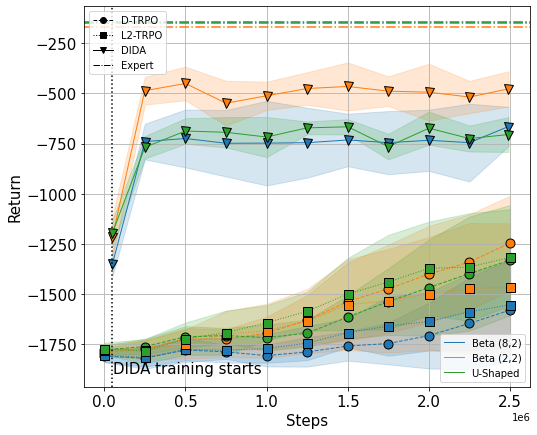
(a) Noises of group 1.

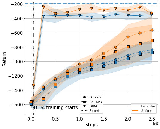
(b) Noises of group 2.

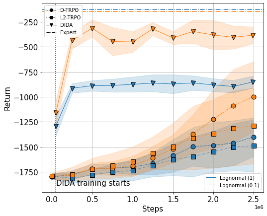
(c) Noises of group 3.

Figure 4: Mean return and one standard deviation (shaded) as a function of the number of steps sampled from the environment for stochastic Pendulum with different noises (10 seeds).

• Group 1: In all these cases, we are considering noises based on beta distributions, with different parameters. We can see in Figure 4(a) that our algorithm is able to achieve a much better performance compared to the ones of the baselines, even with a fraction of the training samples. For every algorithm, the most favourable case seems to be the second one, based on a beta $(2,2)$ noise. This may be because of the features of the other two noises. The first, beta $(8,2)$, is non-zero mean, so that the action is affected, on average, by a translation in one direction. The third one, based on a $\beta(0.5,0.5)$ distribution, is zero-mean, but is characterized by a higher variance than the second ($0.5$ vs $0.2$).

• Group 2: Here again, we see in Figure 4(b) that DIDA is able to get the best performance, even if the two baselines seem to learn much faster than for group 1. This suggest that group 2 contains easier tasks, even though the triangular noise is not symmetric. Still, note that even if the probability of the random action in the first case is small, in the situation of delay it accumulates so that the probability of having a random action inside the action queue of $d=5$ is $1-0.9^{5}\approx 0.41$. Nonetheless, DIDA seems to deal very well with this situation.

• Group 3: Being strongly asymmetric and unbounded, theses noises pose more challenge to the algorithms. We report the results in Figure 4(c). For the Lognormal (1) noise, no algorithm reaches a satisfactory performance. However, again, DIDA obtains the best performance for each noise.

Complement for trading

We illustrate here a specific problem to the trading task, caused by the batch-RL scenario. After some iterations, the policy trained by DIDA overfits the policy of the expert on the training set and its policy on the testing set starts to shift away from the one of the expert. We illustrate this by comparing the plots of the policies for the training set of years 2016-2017 (Figure 5) to the one of the testing set of year 2019 (Figure 6). In these plots, the x-axis represents the time of the day while the y-axis represents the day of the year. The color refers to the action of the agent. This representation clearly shows the daily pattern that the expert has found in the data.

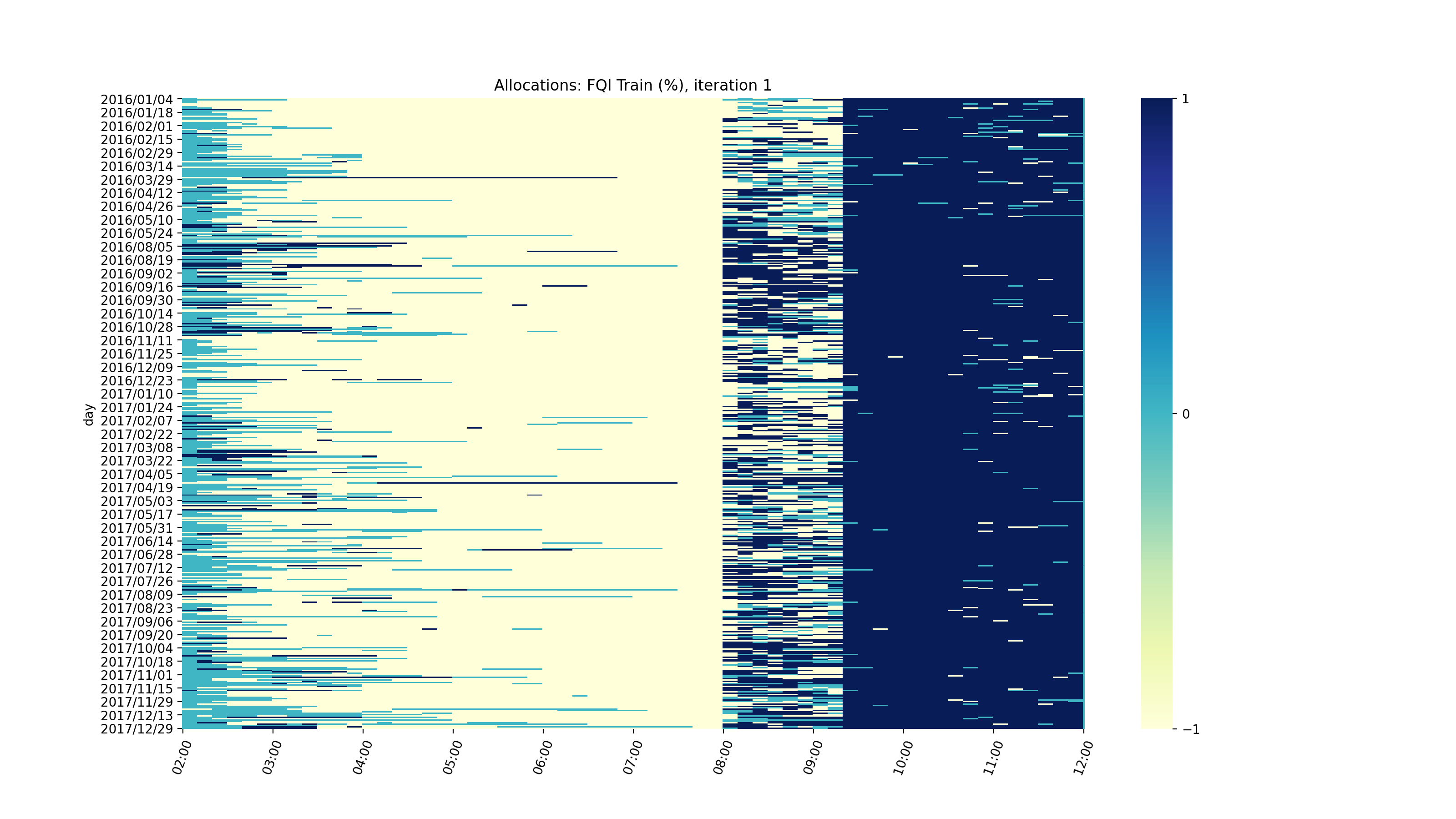
(a) Expert

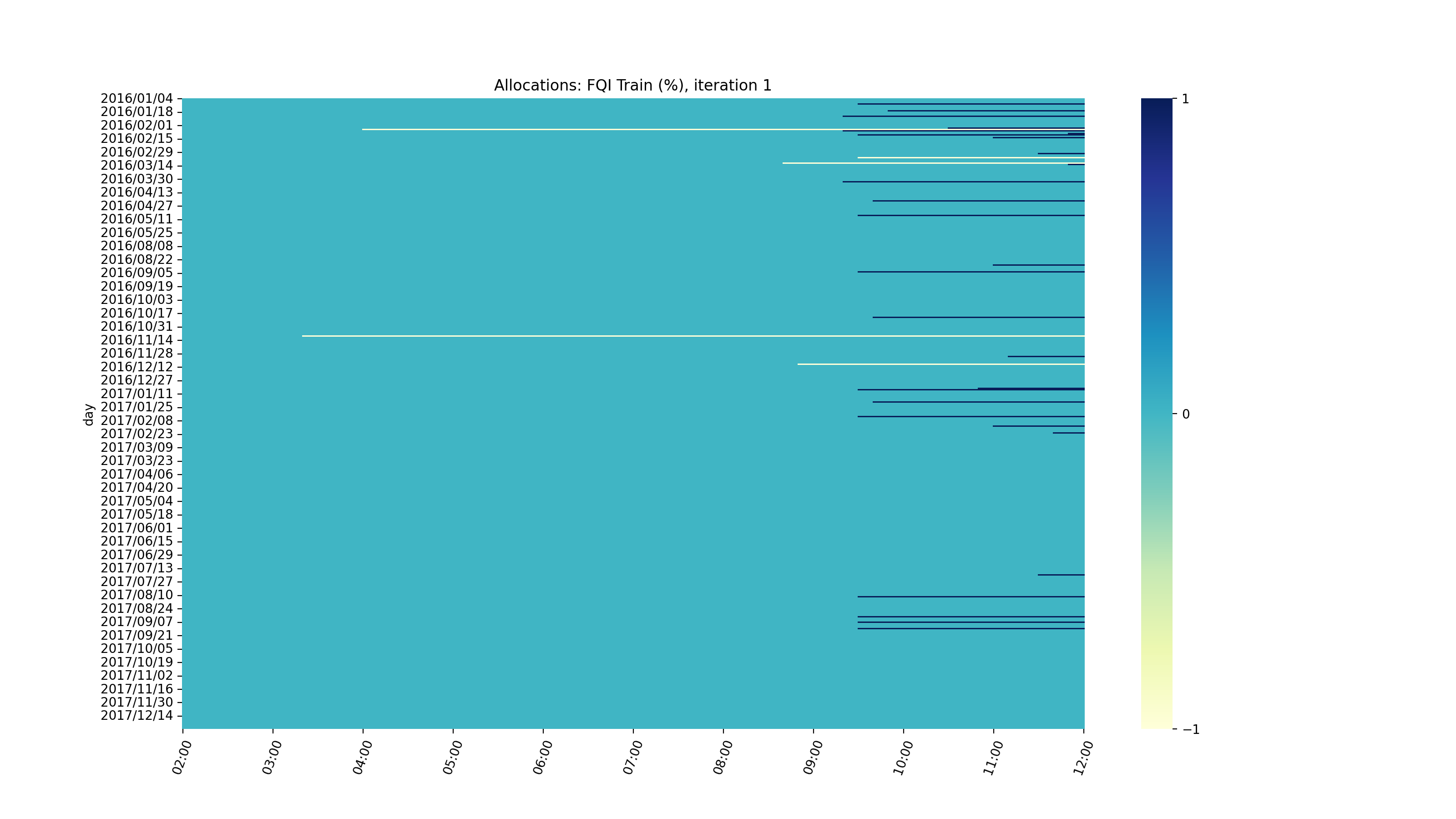
(b) DIDA - Iteration 1

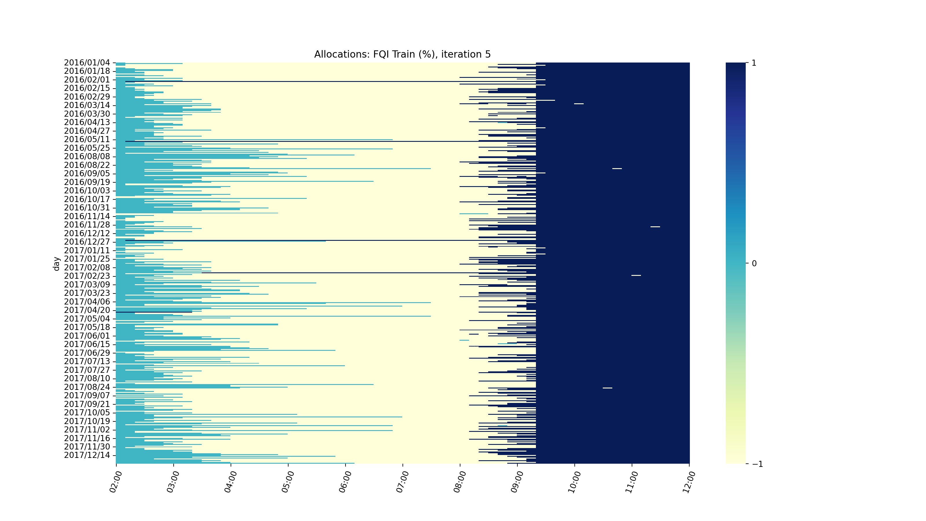
(c) DIDA - Iteration 5

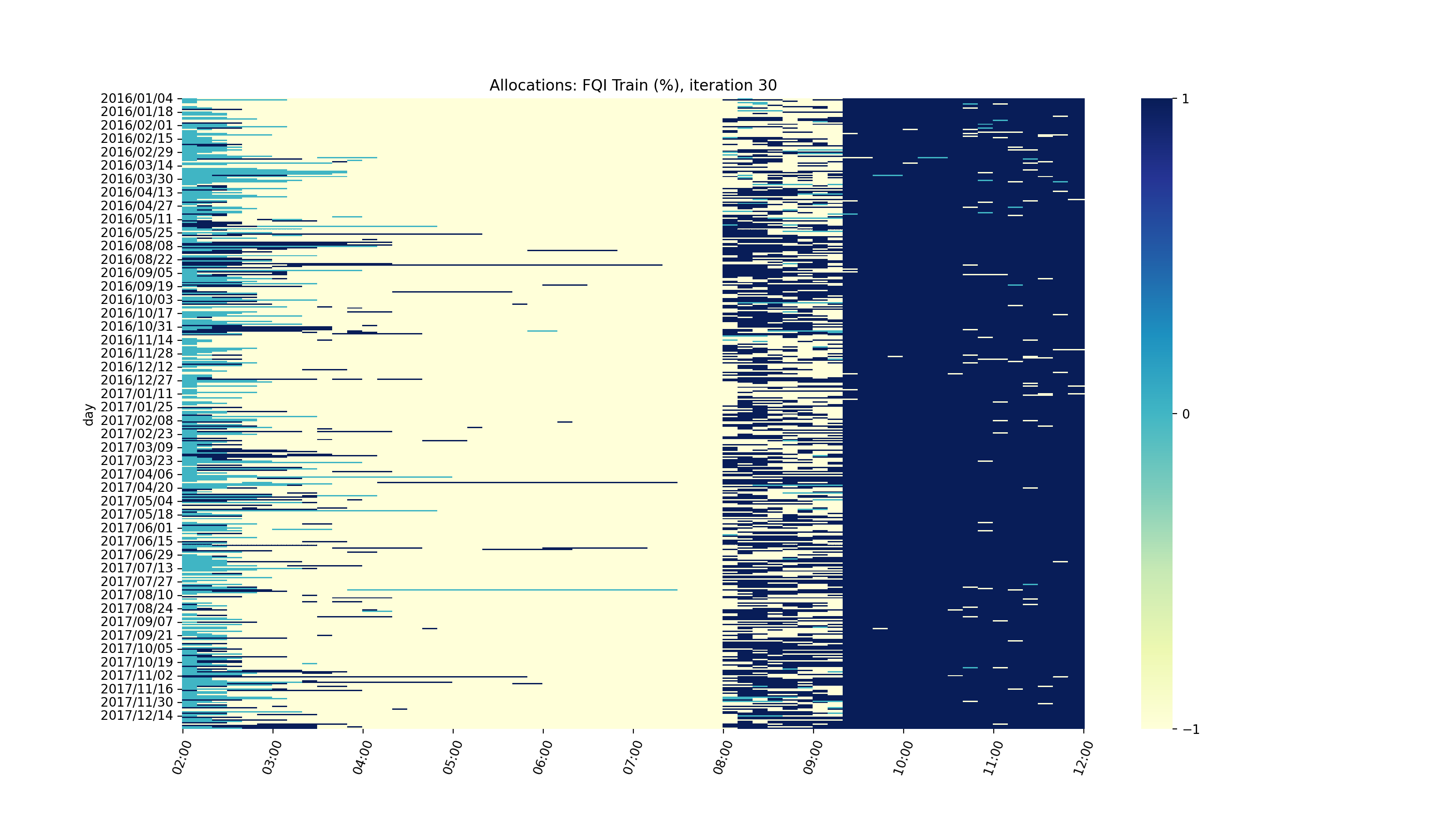
(d) DIDA - Iteration 30

Figure 5: Comparison of the expert’s and DIDA’s policies on the training set (2017-2016)

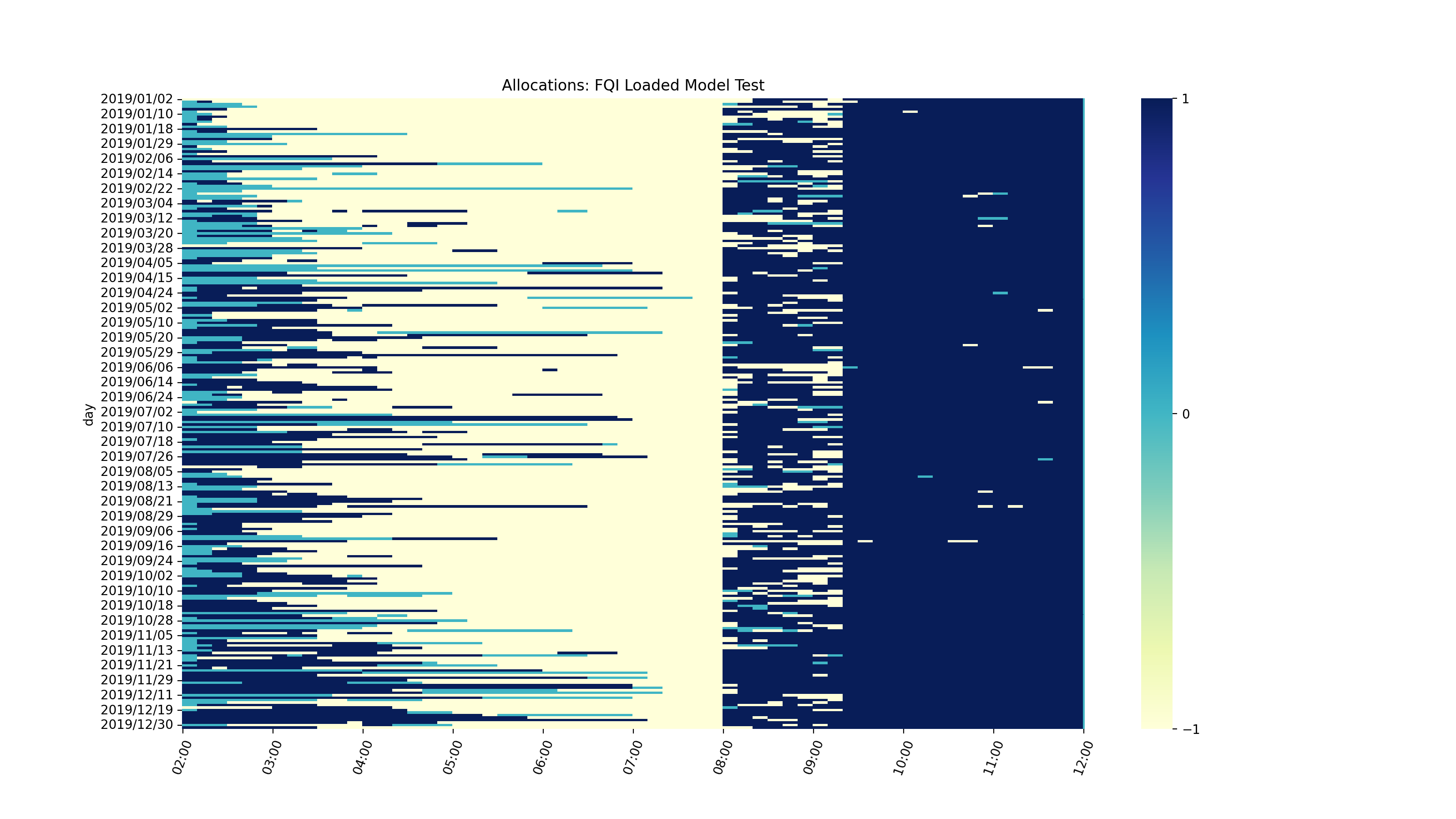
(a) Expert

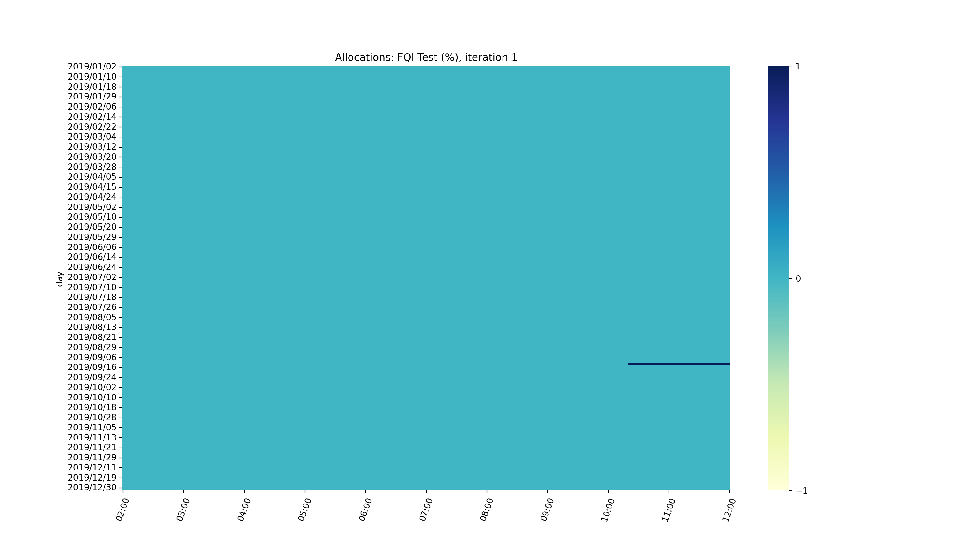
(b) DIDA - Iteration 1

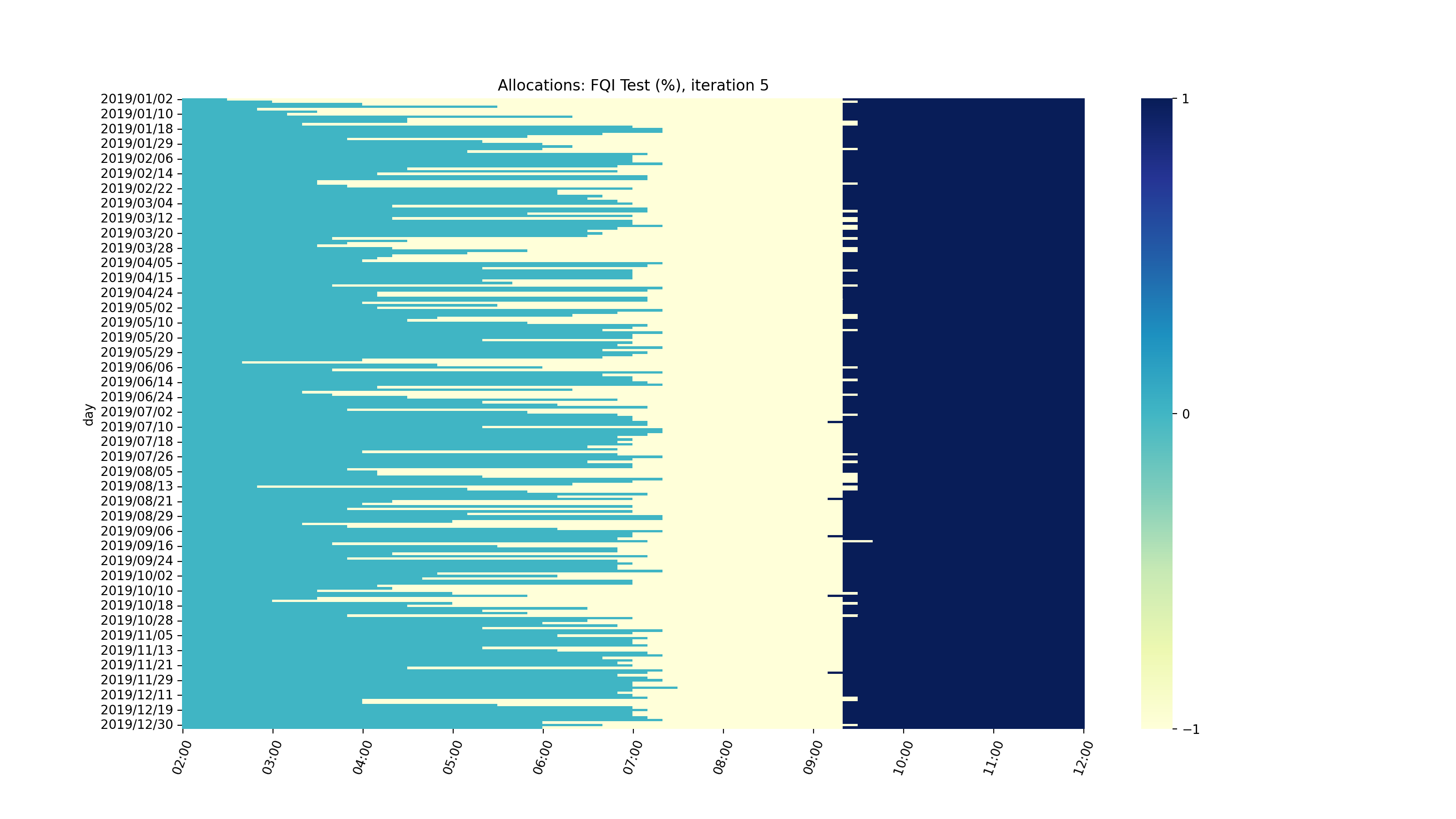
(c) DIDA - Iteration 5

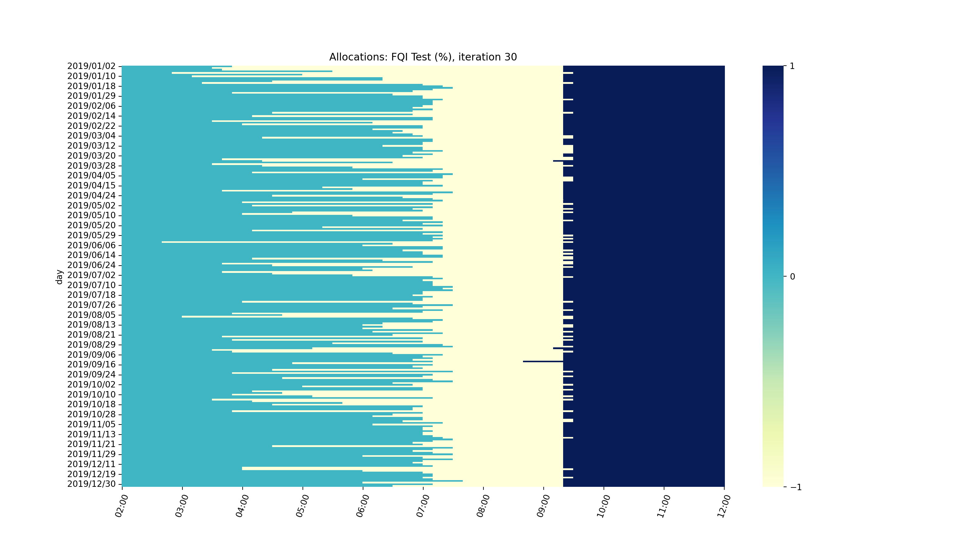
(d) DIDA - Iteration 30

Figure 6: Comparison of the expert’s and DIDA’s policies on the testing set (2019)

References

• Agarwal & Aggarwal (2021) Agarwal, M. and Aggarwal, V. Blind decision making: Reinforcement learning with delayed observations. In Proceedings of the International Conference on Automated Planning and Scheduling, volume 31, pp.  2–6, 2021.
• Altman & Nain (1992) Altman, E. and Nain, P. Closed-loop control with delayed information. ACM sigmetrics performance evaluation review, 20(1):193–204, 1992.
• Bertsekas (1987) Bertsekas, D. P. Dynamic Programming: Determinist. and Stochast. Models. Prentice-Hall, 1987.
• Bisi et al. (2020) Bisi, L., Liotet, P., Sabbioni, L., Reho, G., Montali, N., Restelli, M., and Corno, C. Foreign exchange trading: a risk-averse batch reinforcement learning approach. In Proceedings of the First ACM International Conference on AI in Finance, pp.  1–8, 2020.
• Bouteiller et al. (2020) Bouteiller, Y., Ramstedt, S., Beltrame, G., Pal, C., and Binas, J. Reinforcement learning with random delays. In International Conference on Learning Representations, 2020.
• Brockman et al. (2016) Brockman, G., Cheung, V., Pettersson, L., Schneider, J., Schulman, J., Tang, J., and Zaremba, W. Openai gym, 2016.
• Chen et al. (2021) Chen, B., Xu, M., Li, L., and Zhao, D. Delay-aware model-based reinforcement learning for continuous control. Neurocomputing, 450:119–128, 2021.
• Chen & Guestrin (2016) Chen, T. and Guestrin, C. Xgboost: A scalable tree boosting system. In Proceedings of the 22nd acm sigkdd international conference on knowledge discovery and data mining, pp.  785–794, 2016.
• Derman et al. (2021) Derman, E., Dalal, G., and Mannor, S. Acting in delayed environments with non-stationary markov policies. arXiv preprint arXiv:2101.11992, 2021.
• Droździel et al. (2020) Droździel, P., Tarkowski, S., Rybicka, I., and Wrona, R. Drivers’ reaction time research in the conditions in the real traffic. Open Engineering, 10(1):35–47, 2020.
• Dugard & Verriest (1998) Dugard, L. and Verriest, E. I. Stability and control of time-delay systems, volume 228. Springer, 1998.
• Dulac-Arnold et al. (2019) Dulac-Arnold, G., Mankowitz, D., and Hester, T. Challenges of real-world reinforcement learning. arXiv preprint arXiv:1904.12901, 2019.
• Ernst et al. (2005) Ernst, D., Geurts, P., and Wehenkel, L. Tree-based batch mode reinforcement learning. Journal of Machine Learning Research, 6(Apr):503–556, 2005.
• Firoiu et al. (2018) Firoiu, V., Ju, T., and Tenenbaum, J. At human speed: Deep reinforcement learning with action delay. arXiv preprint arXiv:1810.07286, 2018.
• Geurts et al. (2006) Geurts, P., Ernst, D., and Wehenkel, L. Extremely randomized trees. Machine learning, 63(1):3–42, 2006.
• Gu & Niculescu (2003) Gu, K. and Niculescu, S.-I. Survey on recent results in the stability and control of time-delay systems. J. Dyn. Sys., Meas., Control, 125(2):158–165, 2003.
• Haarnoja et al. (2018) Haarnoja, T., Zhou, A., Abbeel, P., and Levine, S. Soft actor-critic: Off-policy maximum entropy deep reinforcement learning with a stochastic actor. In International conference on machine learning, pp. 1861–1870. PMLR, 2018.
• Kakade & Langford (2002) Kakade, S. and Langford, J. Approximately optimal approximate reinforcement learning. In In Proc. 19th International Conference on Machine Learning. Citeseer, 2002.
• Katsikopoulos & Engelbrecht (2003) Katsikopoulos, K. V. and Engelbrecht, S. E. Markov decision processes with delays and asynchronous cost collection. IEEE transactions on automatic control, 48(4):568–574, 2003.
• Kingma & Ba (2014) Kingma, D. P. and Ba, J. Adam: A method for stochastic optimization. arXiv preprint arXiv:1412.6980, 2014.
• Laskey et al. (2017) Laskey, M., Lee, J., Fox, R., Dragan, A., and Goldberg, K. Dart: Noise injection for robust imitation learning. In Conference on robot learning, pp.  143–156. PMLR, 2017.
• Liotet et al. (2021) Liotet, P., Venneri, E., and Restelli, M. Learning a belief representation for delayed reinforcement learning. In 2021 International Joint Conference on Neural Networks (IJCNN), pp.  1–8. IEEE, 2021.
• Mahmood et al. (2018) Mahmood, A. R., Korenkevych, D., Komer, B. J., and Bergstra, J. Setting up a reinforcement learning task with a real-world robot. In 2018 IEEE/RSJ International Conference on Intelligent Robots and Systems (IROS), pp.  4635–4640. IEEE, 2018.
• Metelli et al. (2020) Metelli, A. M., Mazzolini, F., Bisi, L., Sabbioni, L., and Restelli, M. Control frequency adaptation via action persistence in batch reinforcement learning. In International Conference on Machine Learning, pp. 6862–6873. PMLR, 2020.
• Mysore et al. (2021) Mysore, S., Mabsout, B., Mancuso, R., and Saenko, K. Regularizing action policies for smooth control with reinforcement learning. In 2021 IEEE International Conference on Robotics and Automation (ICRA), pp.  1810–1816. IEEE, 2021.
• Nair & Hinton (2010) Nair, V. and Hinton, G. E. Rectified linear units improve restricted boltzmann machines. In Icml, 2010.
• Osa et al. (2018) Osa, T., Pajarinen, J., Neumann, G., Bagnell, J. A., Abbeel, P., and Peters, J. An algorithmic perspective on imitation learning. arXiv preprint arXiv:1811.06711, 2018.
• Papamakarios et al. (2017) Papamakarios, G., Pavlakou, T., and Murray, I. Masked autoregressive flow for density estimation. arXiv preprint arXiv:1705.07057, 2017.
• Puterman (2014) Puterman, M. L. Markov decision processes: discrete stochastic dynamic programming. John Wiley & Sons, 2014.
• Rachelson & Lagoudakis (2010) Rachelson, E. and Lagoudakis, M. G. On the locality of action domination in sequential decision making. 2010.
• Riva et al. (2021) Riva, A., Bisi, L., Liotet, P., Sabbioni, L., Vittori, E., Pinciroli, M., Trapletti, M., and Restelli, M. Learning fx trading strategies with fqi and persistent actions. 2021.
• Ross & Bagnell (2010) Ross, S. and Bagnell, D. Efficient reductions for imitation learning. In Proceedings of the thirteenth international conference on artificial intelligence and statistics, pp.  661–668. JMLR Workshop and Conference Proceedings, 2010.
• Ross et al. (2011) Ross, S., Gordon, G., and Bagnell, D. A reduction of imitation learning and structured prediction to no-regret online learning. In Proceedings of the fourteenth international conference on artificial intelligence and statistics, pp.  627–635. JMLR Workshop and Conference Proceedings, 2011.
• Schuitema et al. (2010) Schuitema, E., Buşoniu, L., Babuška, R., and Jonker, P. Control delay in reinforcement learning for real-time dynamic systems: a memoryless approach. In 2010 IEEE/RSJ International Conference on Intelligent Robots and Systems, pp.  3226–3231. IEEE, 2010.
• Schulman et al. (2015a) Schulman, J., Levine, S., Abbeel, P., Jordan, M., and Moritz, P. Trust region policy optimization. In International conference on machine learning, pp. 1889–1897. PMLR, 2015a.
• Schulman et al. (2015b) Schulman, J., Moritz, P., Levine, S., Jordan, M., and Abbeel, P. High-dimensional continuous control using generalized advantage estimation. arXiv preprint arXiv:1506.02438, 2015b.
• Sutton & Barto (2018) Sutton, R. S. and Barto, A. G. Reinforcement learning: An introduction. MIT press, 2018.
• Sutton et al. (1999) Sutton, R. S., Precup, D., and Singh, S. Between mdps and semi-mdps: A framework for temporal abstraction in reinforcement learning. Artificial intelligence, 112(1-2):181–211, 1999.
• Todorov et al. (2012) Todorov, E., Erez, T., and Tassa, Y. Mujoco: A physics engine for model-based control. In 2012 IEEE/RSJ International Conference on Intelligent Robots and Systems, pp.  5026–5033. IEEE, 2012.
• Villani (2009) Villani, C. Optimal transport: old and new, volume 338. Springer, 2009.
• Walsh et al. (2009) Walsh, T. J. et al. Learning and planning in environments with delayed feedback. Autonomous Agents and Multi-Agent Systems, 18(1):83, 2009.
• Wilcox (1993) Wilcox, J. W. The effect of transaction costs and delay on performance drag. Financial Analysts Journal, 49(2):45–54, 1993.
• Xu et al. (2020) Xu, T., Li, Z., and Yu, Y. Error bounds of imitating policies and environments. Advances in Neural Information Processing Systems, 33, 2020.