Coherent excitation energy transfer in model photosynthetic reaction center:
Effects of non-Markovian quantum environment

Abstract

Excitation energy transfer (EET) and electron transfer (ET) are crucially involved in photosynthetic processes. In reality, the photosynthetic reaction center constitutes an open quantum system of EET and ET, which manifests an interplay of pigments, solar light and phonon baths. So far theoretical studies have been mainly based on master equation approaches in the Markovian condition. The non-Markovian environmental effect, which may play a crucial role, has not been sufficiently considered. In this work, we propose a mixed dynamic approach to investigate this open system. The influence of phonon bath is treated via the exact dissipaton equation of motion (DEOM) while that of photon bath is via the Lindblad master equation. Specifically, we explore the effect of non-Markovian quantum phonon bath on the coherent transfer dynamics and its manipulation on the current–voltage behavior. Distinguished from the results of completely Markovian Lindblad equation and those adopting classical environment description, the mixed DEOM–Lindblad simulations exhibit transfer coherence up to a few hundreds femtoseconds and the related environmental manipulation effect on current. These non-Markovian quantum coherent effects may be extended to more complex and realistic systems and be helpful to the design of organic photovoltaic devices.

I Introduction

Photosynthesis is one of the most important processes in biological systems, by which plants and other organisms convert sunlight energy into chemical energy. It is found that excitation energy transfer (EET) and electron transfer (ET) are crucially involved in the photosynthetic process. To be concrete, sunlight is absorbed to create an excited state, followed by EET along pigments to reaction center, where ET happens resulting in charge separation converting excitation energy to chemical energy.

In recent years, the role of quantum coherence in the EET and ET processes of photosynthesis has got great interest.Pol220953 ; Cao204888 ; Rom17355 ; Rom14676 ; Ful14706 ; Rom104300 ; Col10644 ; Eng07782 ; Lee071462 The core complex is the main participant in the EET and ET processes of reaction center. In reality, it constitutes an open quantum system, which manifests an interplay among pigments, solar light and phonon baths. The involved dynamics could be non-Markovian in case that the coupling strength between pigments and the phonon environment be comparable to that between pigments themselves, as well as the timescale of EET/ET around that of the phonon bath memory.

Unlike the light-harvesting systems, which have been theoretically intensively studied,Ish09234111 ; Kre112166 ; Che11194508 ; Xu13024106 ; Che1569 ; Zha16204109 ; Jan18035003 ; Kun208783 ; Yan211498 ; Kun22349 dynamics of the EET/ET processes in the reaction center is relatively rarely explored. So far theoretical studies on EET/ET in the photosynthetic reaction center are mainly based on some approximate methods in the Markovian condition, such as the Redfield equation,Rom14676 ; Wer18084112 polaron master equation,Qin17012125 Lindblad equation,Kil15155102 and Pauli master equation.Cre13253601 The quantum coherence enhanced effect on electric current was once exhibited in Ref. Dor132746, . However, Creatore and co-workers pointed out that the solutions in Ref. Dor132746, were unstable and the numerical evolutions there did not retain the positivity of density matrix, resulting in artificial behaviors which would diverge with time going on, see the details in Supplemental Material of Ref. Cre13253601, . Hence accurate simulations are needed, together with assessments on approximate approaches.

In this work, we study this open system problem using a mixed dynamic approach. The photon bath (light) influence is treated adopting the Lindblad equation,Lin76119 ; Gor76821 while that of the phonon environment is via the dissipaton equation of motion (DEOM) method.Yan14054105 ; Zha15024112 The DEOM is a non-Markovian and nonperturbative approach, constructed on basis of a quasi-particle, dissipaton representation for hybridized collective bath dynamics. For reduced system dynamics, the DEOM is equivalent to the hierarchical equation of motion (HEOM) formalism,Tan20020901 which is established via time derivative on the influence functional path integral or stochastic fields methods.Tan89101 ; Yan04216 ; Ish053131 ; Xu05041103 ; Xu07031107 Both HEOM and DEOM are exact under Gaussian bath statistics. The DEOM is more convenient and straightforward to study environmental dynamics related problems, such as polarizations under external fields.Zha15024112 ; Zha16204109 ; Che21244105

In numerical demonstrations, the phonon bath will also be treated via the semigroup Lindblad master equation for comparison with DEOM. In this way the effects of quantum coherence versus non-Markovian phonon bath will be highlighted. The remainder of paper is organized as follows. In Sec. II.1, we introduce a five–level modelRom104300 ; Dor132746 ; Kil15155102 ; Cre13253601 ; Qin17012125 applied in our study, which captures the main features of the EET and ET processes in the photosynthetic reaction center. The associated Hamiltonian and bath functions are then described. The mixed DEOM–Lindblad dynamic equations are proposed in Sec. II.2. The construction of Lindblad master equation is briefly outlined in Appendix. Numerical simulations on transfer dynamics and current–voltage behaviors are demonstrated and discussed in Sec. III. We summarize the paper in Sec. IV.

II Theoretical description

In this section, we begin with the setup of total system–plus–baths composite exploited in this study, where the system is described by a five–level model. Rom104300 ; Dor132746 ; Kil15155102 ; Cre13253601 ; Qin17012125 This five–level model system, based on the photosystem II core complex, not only characterizes the main features of EET and ET processes, but also takes into account the important interactions involved. The system Hamiltonian and bath coupling statistics as well as the proposed mixed DEOM–Lindblad dynamic approach are given after that. For brevity, we set $\hbar=1$ and $\beta=1/(k_{B}T)$ throughout the paper, with $k_{B}$ being the Boltzmann constant and $T$ the temperature.

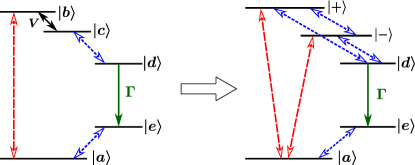
Figure 1: Sketch of the total composite model before and after the diagonalization of system Hamiltonian.

II.1 Five–site model of system and bath statistics

Let us first introduce the system from the biological perspective. Rom104300 The photosystem II reaction center core complex contains four chlorophylls (special pair P_D1 and P_D2 and accessory chlorophylls Chl_D1 and Chl_D2) and two pheophytins (Phe_D1 and Phe_D2), arranged into two branches (D1 and D2). Only the D1 branch plays an active role in the photo-induced electron transfer:

$$\begin{array}[]{ccc}|a\rangle\!:{\rm P}_{\rm D1}{\rm Chl}_{\rm D1}{\rm Phe}_{\rm D1}&\longrightarrow&({\rm P}_{\rm D1})^{\ast}{\rm Chl}_{\rm D1}{\rm Phe}_{\rm D1}\!:|b\rangle\\ e\rightsquigarrow\ \uparrow&&\downarrow\\ |e\rangle\!:{\rm P}_{\rm D1}^{+}{\rm Chl}_{\rm D1}{\rm Phe}_{\rm D1}&&{\rm P}_{\rm D1}({\rm Chl}_{\rm D1}{\rm Phe}_{\rm D1})^{\ast}\!:|c\rangle\\ e\mathrel{\mathchoice{\reflectbox{$\displaystyle\rightsquigarrow$}}{\reflectbox{$\textstyle\rightsquigarrow$}}{\reflectbox{$\scriptstyle\rightsquigarrow$}}{\reflectbox{$\scriptscriptstyle\rightsquigarrow$}}}\ \uparrow&&\downarrow\\ \ \ \ \ \ \ \ {\rm P}_{\rm D1}^{+}{\rm Chl}_{\rm D1}{\rm Phe}_{\rm D1}^{-}&\longleftarrow&\,{\rm P}_{\rm D1}{\rm Chl}_{\rm D1}^{+}{\rm Phe}_{\rm D1}^{-}\ \ \ \ \ \ |d\rangle\\ \end{array}$$

The D1 branch, ${\rm P}_{\rm D1}{\rm Chl}_{\rm D1}{\rm Phe}_{\rm D1}$, is firstly excited from $|a\rangle$ to $|b\rangle$ via the absorption of photons. From $|b\rangle$ to $|c\rangle$ is the EET, followed by the charge separation resulting in state $|d\rangle$ where the positive and negative charges are rapidly spatially separated. For simplicity, a charge–separated state $|d\rangle$ is coarsely used to represent both states. From $|d\rangle$ to $|e\rangle$, an electron is released from the system. At last, the system captures an electron from the surroundings to complete the cycle and returns to the ground state $|a\rangle$.

According to the above description, the system Hamiltonian can be written as

$$H_{\mbox{\tiny S}}=\sum_{m\in I}E_{m}|m\rangle\langle m|+V(|b\rangle\langle c|+|c\rangle\langle b|),$$ (1)

with $I\equiv\{a,b,c,d,e\}$. To phenomenologically describe the electron release from $|d\rangle$ to $|e\rangle$, a superoperator can be introduced asDor132746 ; Kil15155102 ; Cre13253601 ; Qin17012125

$$L_{\Gamma}{\hat{O}}=-\frac{\Gamma}{2}\big{[}{\hat{O}}|d\rangle\langle d|+|d\rangle\langle d|{\hat{O}}-2|e\rangle\langle d|{\hat{O}}|d\rangle\langle e|\big{]}.$$ (2)

Here, $\Gamma$ is the rate of release. In square brackets of Eq. (2), the last term and the first two terms correspond to $T_{1}$ relaxation and $T_{2}$ dephasing, respectively.Red651 ; Yan002068 In this work, we exploit this constant rate description as in literature,Dor132746 ; Kil15155102 ; Cre13253601 ; Qin17012125 to phenomenologically represent the process from $|d\rangle$ to $|e\rangle$. This description is widely applied in various fields, such as chemical kinetics and radioactive decay processes, where the inverse processes rarely happen. In the photosynthetic reaction center, a series of chemical reactions are driven by the electron released from $|d\rangle$ and finally reach $|e\rangle$, while the inverse process from $|e\rangle$ to $|d\rangle$ is almost prohibited.

For the system–plus–baths composite, the total Hamiltonian reads

$$H_{\mbox{\tiny T}}=H_{\mbox{\tiny S}}+H_{\mbox{\tiny SB}}^{(\rm I)}+H_{\mbox{\tiny SB}}^{(\rm II)}+h_{\mbox{\tiny B}}^{(\rm I)}+h_{\mbox{\tiny B}}^{(\rm II)}.$$ (3)

Here, the system Hamiltonian is as in Eq. (1), while the bath Hamiltonians are

$$h_{\mbox{\tiny B}}^{(\rm I)}=\sum_{k}\varepsilon_{k}b_{k}^{\dagger}b_{k}\quad{\rm and}\quad h_{\mbox{\tiny B}}^{(\rm II)}=\sum_{j}\omega_{j}a_{j}^{\dagger}a_{j}$$ (4)

for the photon bath and phonon bath, respectively. The system-bath interaction Hamiltonians read

$$H_{\mbox{\tiny SB}}^{(\rm I)} =\hat{Q}_{1}^{(\textup{\rm I})}\hat{F}_{1}^{(\textup{\rm I})},$$ (5a)

$$H_{\mbox{\tiny SB}}^{(\rm II)} =\sum_{\mu=2}^{5}\hat{Q}_{\mu}^{(\textup{\rm II})}\hat{F}_{\mu}^{(\textup{\rm II})},$$ (5b)

with $\hat{Q}_{1}^{(\textup{\rm I})}=|a\rangle\langle b|+|b\rangle\langle a|$, $\hat{Q}_{2}^{(\textup{\rm II})}=|c\rangle\langle d|+|d\rangle\langle c|$, $\hat{Q}_{3}^{(\textup{\rm II})}=|e\rangle\langle a|+|a\rangle\langle e|$, $\hat{Q}_{4}^{(\textup{\rm II})}=|b\rangle\langle b|$, and $\hat{Q}_{5}^{(\textup{\rm II})}=|c\rangle\langle c|$, whereas $\hat{F}_{1}^{(\textup{\rm I})}=\frac{1}{\sqrt{2}}\sum_{k}\tilde{c}_{k}(b_{k}+b_{k}^{\dagger})$ and $\hat{F}^{(\textup{\rm II})}_{\mu=2\sim 5}=\frac{1}{\sqrt{2}}\sum_{j}c_{\mu j}(a_{j}+a_{j}^{\dagger})$. These settings are depicted in the left panel of Fig. 1 and constitute Gaussian bath couplings. Their influences on the system can be completely characterized by the spectral densities,

$$J_{1}^{(\textup{\rm I})}(\omega>0)=\frac{\pi}{2}\sum_{k}\tilde{c}_{k}^{2}\delta(\omega-\varepsilon_{k}),$$ (6a)

and (for $$\mu,\nu=2\sim 5$$)

$$J_{\mu\nu}^{(\textup{\rm II})}(\omega>0)=\frac{\pi}{2}\sum_{j}c_{\mu j}c_{\nu j}\delta(\omega-\omega_{j}).$$ (6b)

In Fig. 1, red and blue dash arrows represent the state transfers induced by photon and phonon baths, respectively. The system Hamiltonian eigenstates are $|a\rangle$, $|d\rangle$, $|e\rangle$ and

$$\begin{bmatrix}|+\rangle\\ |-\rangle\end{bmatrix}={\bf U}\begin{bmatrix}|b\rangle\\ |c\rangle\end{bmatrix}\equiv\begin{bmatrix}u_{11}&u_{12}\\ u_{21}&u_{22}\end{bmatrix}\begin{bmatrix}|b\rangle\\ |c\rangle\end{bmatrix}$$ (7)

with $\bf U$ being the real and orthogonal transformation matrix which diagonalizes $H_{\mbox{\tiny S}}$. Inversely

$$\begin{bmatrix}|b\rangle\\ |c\rangle\end{bmatrix}=\begin{bmatrix}u_{11}&u_{21}\\ u_{12}&u_{22}\end{bmatrix}\begin{bmatrix}|+\rangle\\ |-\rangle\end{bmatrix}.$$ (8)

Correspondingly, we can recast

$$\hat{Q}_{1}^{(\textup{\rm I})}=u_{11}\big{(}|a\rangle\langle+|+|+\rangle\langle a|\big{)}+u_{21}\big{(}|a\rangle\langle-|+|-\rangle\langle a|\big{)},$$

$$\hat{Q}_{2}^{(\textup{\rm II})}=u_{12}\big{(}|+\rangle\langle d|+|d\rangle\langle+|\big{)}+u_{22}\big{(}|-\rangle\langle d|+|d\rangle\langle-|\big{)},$$

$$\hat{Q}_{4}^{(\textup{\rm II})}=u^{2}_{11}|+\rangle\langle+|+u^{2}_{21}|-\rangle\langle-|+u_{11}u_{21}\big{(}|+\rangle\langle-|+|-\rangle\langle+|\big{)},$$

$$\hat{Q}_{5}^{(\textup{\rm II})}=u^{2}_{12}|+\rangle\langle+|+u^{2}_{22}|-\rangle\langle-|+u_{12}u_{22}\big{(}|+\rangle\langle-|+|-\rangle\langle+|\big{)},$$

and $\hat{Q}_{3}^{(\textup{\rm II})}$ is not affected. The transformed interaction patterns are exhibited in the right panel of Fig. 1.

II.2 Mixed DEOM–Lindblad dynamic approach

In the total composite space, the total density operator $\rho_{\mbox{\tiny T}}(t)$ evolves as

$$\dot{\rho}_{\mbox{\tiny T}}(t)=-i[H_{\mbox{\tiny T}},\rho_{\mbox{\tiny T}}(t)]+L_{\Gamma}\rho_{\mbox{\tiny T}}(t),$$ (9)

with $H_{\mbox{\tiny T}}$ and $L_{\Gamma}$ defined in Eqs. (3) and (2), respectively. In the proposed mixed dynamic approach, light is treated as photon bath via the Lindblad master equation, detailed in Appendix. Thus an additional superoperator for the action of light is now introduced as

$$L^{(\textup{\rm I})}=\gamma_{+}u_{11}^{2}L_{+}+\gamma_{-}u_{21}^{2}L_{-}\,,$$ (10)

with $\gamma_{\pm}\equiv 2J_{1}^{(\textup{\rm I})}(\omega_{\pm a})$ the dissipative rate and

$$L_{\pm}\hat{O} =(1+\bar{n}_{\pm})\Big{(}\langle\pm|\hat{O}|\pm\rangle\,|a\rangle\langle a|-\frac{1}{2}\big{\{}|\pm\rangle\langle\pm|,\hat{O}\big{\}}\Big{)}$$

$$\quad+\bar{n}_{\pm}\Big{(}\langle a|\hat{O}|a\rangle\,|\pm\rangle\langle\pm|-\frac{1}{2}\big{\{}|a\rangle\langle a|,\hat{O}\big{\}}\Big{)},$$ (11)

where $\bar{n}_{\pm}\equiv\bar{n}_{\pm a}$; cf. Appendix.

To explore non-Markovian and non-perturbative influence of phonon bath, we adopt the well-established DEOM approach. It starts with the exponential expansion form of bath coupling correlation functions,

$$\widetilde{C}_{\mu\nu}^{(\textup{\rm II})}(t)=\frac{1}{\pi}\int^{\infty}_{-\infty}{\rm d}\omega\frac{e^{-i\omega t}J_{\mu\nu}^{(\textup{\rm II})}(\omega)}{1-e^{-\beta\omega}}=\sum_{\kappa}\xi^{\mu\nu}_{\kappa}e^{-\gamma^{\mu\nu}_{\kappa}t}\,.$$ (12)

The first identity is the fluctuation–dissipation theorem.Wei21 ; Yan05187 The standard DEOM algebra gives rise toYan14054105 ; Zha15024112

$$\dot{\rho}^{(n)}_{\bf n} =-\Big{[}i{\cal L}_{\mbox{\tiny S}}-L_{\Gamma}-L^{(\textup{\rm I})}+\sum_{\mu\nu\kappa}n^{\mu\nu}_{\kappa}\gamma^{\mu\nu}_{\kappa}\Big{]}\rho^{(n)}_{\bf n}$$

$$\quad-i\sum_{\mu\nu\kappa}\Big{[}{\cal A}_{\mu}\rho^{(n+1)}_{{\bf n}_{\mu\nu\kappa}^{+}}+n^{\mu\nu}_{\kappa}{\cal C}^{\mu\nu}_{\kappa}\rho^{(n-1)}_{{\bf n}_{\mu\nu\kappa}^{-}}\Big{]},$$ (13)

with ${\cal L}_{\mbox{\tiny S}}\hat{O}\equiv[H_{\mbox{\tiny S}},\hat{O}]$ and

$${\cal A}_{\mu}\hat{O} \equiv[\hat{Q}_{\mu}^{(\textup{\rm II})},\hat{O}],$$ (14a)

$${\cal C}^{\mu\nu}_{\kappa}\hat{O} \equiv\xi^{\mu\nu}_{\kappa}\hat{Q}_{\nu}^{(\textup{\rm II})}\hat{O}-\big{(}\xi^{\mu\nu}_{\bar{\kappa}}\big{)}^{\ast}\hat{O}\hat{Q}_{\nu}^{(\textup{\rm II})}.$$ (14b)

This is the mixed DEOM–Lindblad formalism. The term of index $\bar{\kappa}$ is associated with that of $\kappa$ by $\gamma^{\mu\nu}_{\bar{\kappa}}\equiv(\gamma^{\mu\nu}_{\kappa})^{\ast}$. The indices of density matrices are denoted as $\textbf{n}=\{n^{\mu\nu}_{\kappa}\}$, an ordered set of the bosonic dissipaton’s occupation numbers, $n^{\mu\nu}_{\kappa}=0,1,\cdots$, and $n=\sum_{\mu\nu\kappa}n^{\mu\nu}_{\kappa}$ the total number. ${\bf n}^{\pm}_{\mu\nu\kappa}$ differs from ${\bf n}$ only at the specified $n^{\mu\nu}_{\kappa}$ by $\pm 1$. $\rho^{(0)}_{\bf 0}$ is just the reduced system density operator, while the others, $\rho^{(n\geq 1)}_{\bf n}$, coupled to $\rho^{(0)}_{\bf 0}$ in a hierarchical manner, are dissipaton density operators.

III Numerical demonstrations and discussions

For numerical simulations, we adopt the Drude model for the phonon bath spectral densities (for $\mu,\nu=2\sim 5$),

$$J_{\mu\nu}^{(\textup{\rm II})}(\omega)=\frac{2\eta_{\mu\nu}\lambda_{\nu}\gamma_{\nu}\omega}{\omega^{2}+\gamma_{\nu}^{2}}\,.$$ (15)

The Drude model is a strongly overdamped solvent model. In Eq. (15), $\lambda_{\nu}$ is the reorganization energy and $\gamma_{\nu}$ is the damping rate. $\{\eta_{\mu\nu}\}$ should form a positive–definite matrix. It characterizes the correlation between different dissipative modes, cf. Eq. (6b). Here, the way of denoting cross–correlation contributions is essentially the same as in Ref. Ish10055004, . We set parameters as in Table. 1. They are selected in accordance with Refs. Kil15155102, ; Cre13253601, ; Dor132746, . Particularly, the photon average occupation paramter, $\bar{n}_{\pm}$, is chosen to be $60000$, to match with Refs. Kil15155102, ; Cre13253601, ; Dor132746, . As pointed out in Ref. Kil15155102, , this represents solar energy concentration within the antenna and is not related to the actual physical temperature of photon bath.

Parameters	Units	Values
$E_{a}$	cm-1	0
$E_{b}$	cm-1	14856
$E_{c}$	cm-1	14736
$E_{d}$	cm-1	13245
$E_{e}$	cm-1	1611
$V$	cm-1	30
$\gamma_{\pm}$	cm-1	0.005
$\bar{n}_{\pm}$		60000
$T$	K	300
$\lambda_{2}$	cm-1	140
$\gamma_{2}$	cm-1	140
$\lambda_{3}$	cm-1	200
$\gamma_{3}$	cm-1	200
$\lambda_{4}$	cm-1	100
$\gamma_{4}$	cm-1	10
$\lambda_{5}$	cm-1	100
$\gamma_{5}$	cm-1	10

Table 1: Parameters used in the simulations.

The setup of system Hamiltonian results in the following ${\bf U}$–matrix in Eq. (7),

$${\bf U}=\begin{bmatrix}0.973&-0.230\\ 0.230&0.973\end{bmatrix}.$$

In simulations, the $\{\eta_{\mu\nu}\}$ parameters are set as

$$\begin{bmatrix}\eta_{22}&\eta_{23}&\eta_{24}&\eta_{25}\\ \eta_{32}&\eta_{33}&\eta_{34}&\eta_{35}\\ \eta_{42}&\eta_{43}&\eta_{44}&\eta_{45}\\ \eta_{52}&\eta_{53}&\eta_{54}&\eta_{55}\end{bmatrix}=\begin{bmatrix}1&0&0&0\\ 0&1&0&0\\ 0&0&1&\eta\\ 0&0&\eta&1\end{bmatrix}.$$

We choose $\eta=1$ and $\eta=-1$ to represent the fully correlated and anti–correlated scenarios of the involved two fluctuating modes, $\hat{Q}_{4}^{(\textup{\rm II})}=|b\rangle\langle b|$ and $\hat{Q}_{5}^{(\textup{\rm II})}=|c\rangle\langle c|$, respectively. Note their real effects shall be considered with the eigenstates of system and may be different if the sign and value of the coherent coupling $V$ change. The $\Gamma$ parameter in Eq. (2) will be varied in the following demonstration.

Before numerical discussions, it is worth to clarify that non-Markovian quantum nature is basically the real physical characteristics of phonon environments. Whether the caused effect is important or not theoretically depends on parameters.Xu079618 ; Din12224103 When approximate treatments are adopted, validity is to be assessed by comparing with accurate methods. Meanwhile the existing difference in such comparisons would reflect the feature of the neglected factor in those approximate approaches. In the following part of this section, the completely Markovian Lindblad equation or methods adopting classical environment description will be assessed via comparison to the simulation results given by the mixed DEOM–Lindblad approach. The effects of non-Markovian quantum phonon environment can then be analyzed in due course.

Figures 2 and 3 depict the transient dynamics obtained from different approaches. We choose cases where $\Gamma=100$ and $500$ cm^-1, both simulated for $\eta=-1$ and $\eta=1$. The system is set to be at $|a\rangle$ initially. The black-solid, DEOM curves are evaluated via the mixed DEOM–Lindblad formalism proposed in Sec. II.2. Both the expansion of phonon bath correlation functions and the hierarchy of dynamic equations are converged. To explore the quantum phonon environment effects, results from the classical bath correspondence are illustrated with the red-dot curves for comparison. In the classical bath condition, the involved bath correlations are real functions. Thus, the difference of red-dot curves to the black-solid ones is due to neglecting the imaginary parts of the second identity of Eq. (12). The blue-dash, Lindblad results are obtained by applying the Lindblad master equation for both photon and phonon bath operations, cf. Eqs. (29)–(30) of Appendix. Note the Pauli master equation adopted in Ref. Cre13253601, neglects the off-diagonal elements of system density matrix. It corresponds to the Lindblad equation of Eq. (29) subject to a population projection. Therefore the non-Markovian correlated environmental effects can be highlighted in comparison between black-solid and blue-dash curves.

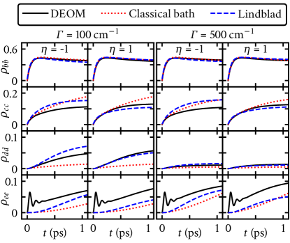
Figure 2: Population evolutions evaluated via the mixed DEOM–Lindblad (black-solid), DEOM–Lindblad under the classical bath limit (red-dot), and complete Lindblad (blue-dash) methods with varied $\Gamma$ and $\eta$ parameters.

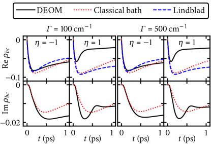
Figure 3: Decoherence during EET between the states $|b\rangle$ and $|c\rangle$, evaluated via the mixed DEOM–Lindblad (black-solid), DEOM–Lindblad under the classical bath limit (red-dot), and complete Lindblad (blue-dash) methods with varied $\Gamma$ and $\eta$ parameters.

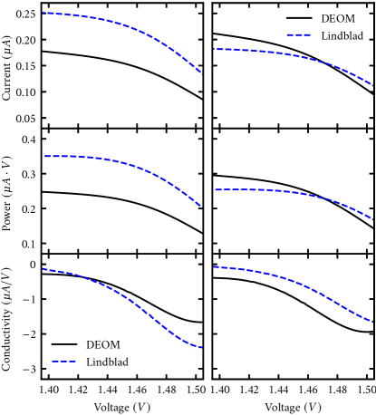
Figure 4: Current, power, and conductivity versus the effective voltage with the $\Gamma$ parameter varied. The black solid curves are from the mixed DEOM–Lindblad simulations while the blue dash curves are from the complete Lindblad simulations.

In Fig. 2, the mixed DEOM–Lindblad (black-solid) simulations exhibit quantum coherence in the panels of $\rho_{ee}$. Both the complete Lindblad (blue-dash) and classical bath (red-dot) results show little quantum coherent behavior, similar as the time evolutions demonstrated in Supplemental Material of Ref. Cre13253601, . The associated decoherence processes of $\rho_{bc}$ are depicted in Fig. 3. There are no Lindblad (blue-dash) curves in the panels of ${\rm Im}\rho_{bc}$, because its results retain zero from the chosen initial state. It is observed that by the mixed DEOM–Lindblad (black-solid) simulations, the anti–correlated bath fluctuations with $\eta=-1$ lead to faster dephasing processes than the correlated ones with $\eta=1$, for the present system. In both Fig. 2 and Fig. 3, the $\Gamma=100$ and $500$ cm^-1 cases give similar transient behaviors except for $\rho_{dd}$ [cf. Eq. (2) and comments after it]. Further effects of $\Gamma$ and $\eta$ on steady states and the associated current–voltage properties are to be demonstrated in Fig. 4.

As in the literature,Rom104300 ; Dor132746 ; Kil15155102 ; Cre13253601 ; Qin17012125 we may view the composite as a biological heat engine, with the steady-state current,

$$j=e\Gamma\rho_{\mbox{\tiny S};dd}^{\rm st}\,,$$ (16)

and the effective voltage $\Phi$ via

$$e\Phi=E_{d}-E_{e}+k_{B}T\ln\frac{\rho_{\mbox{\tiny S};dd}^{\rm st}}{\rho_{\mbox{\tiny S};ee}^{\rm st}}\,.$$ (17)

Here, $e$ is the electron charge. Figure 4 depicts the current (upper-panels), power $j\cdot\Phi$ (middle-panels), and conductivity ${\rm d}j/{\rm d}\Phi$ (lower-panels) versus the voltage, for the results from the mixed DEOM–Lindblad (black-solid) and complete Lindblad (blue-dash) simulations. The current and voltage, $j$ and $\Phi$, are evaluated from Eq. (16) and Eq. (17), respectively, with the $\Gamma$ parameter varied from 600 down to 8 cm^-1 for the mixed DEOM–Lindblad, and 900 down to 12 cm^-1 for the complete Lindblad simulations. Note that under the classical bath condition, $\rho_{\mbox{\tiny S};dd}^{\rm st}=0$, leading to both current and voltage undefined. Negative conductivity is observed owing to the setup of the present model heat engine.

In Fig. 4, the mixed DEOM–Lindblad results show certain manipulation effects by adjusting the cross–correlation, $\eta$–parameter, between different environmental couplings. The current evaluated via the mixed DEOM–Lindblad simulation (black-solid) is overall enlarged in the $\eta=1$ case (upper–right panel) compared with $\eta=-1$ (upper–left panel). This observation highlights the relationship among the non-Markovian quantum environment, the transfer coherence, and the current enhancement. Recall that we have shown in Fig. 3 the former case possesses a longer time of coherence than the latter one. In contrast, since the non-Markovianity and quantum coherence are not fully covered in the complete Lindblad approach, it produces the opposite behaviors that the current is weakened in the $\eta=1$ case in comparison with $\eta=-1$, as seen from the blue-dash curves in the upper panels of Fig. 4.

IV Summary

In this work, we propose a mixed DEOM–Lindblad approach to study the transient dynamics and steady-state current–voltage behaviors of a model photosynthetic reaction center system. The photon bath (light) influence is treated via the Lindblad dissipative superoperator while that of the phonon environment is via the exact DEOM method taking into account the non-Markovian and non-perturbative effects. The correlation between photon and phonon baths’ couplings on the reduced system are also included in the construction of the mixed DEOM–Lindblad formalism. The transfer dynamics and steady-state current–voltage behaviors are compared among different approaches, the mixed DEOM–Lindblad, complete Lindblad, and DEOM–Lindblad with classical bath limit, to explore the non-Markovian quantum environment effects. Distinguished from the other two methods, results via the mixed DEOM–Lindblad simulation exhibit the transfer coherence up to a few hundreds femtoseconds and an environment manipulation effect on the current enhancement. As DEOM is an accurate method, the present observations of non-Markovian quantum coherent effects are expected to be extended to more complex and realistic systems and be helpful to the design of organic photovoltaic devices.

Appendix: Constructional detail of Lindblad master equation

In this appendix, we give the constructional detail of the Lindblad master equation. Consider a general form of system–plus–bath total Hamiltonian,

$$H_{\mbox{\tiny T}}=H_{\mbox{\tiny S}}+\sum_{\mu}\hat{Q}_{\mu}^{\mbox{\tiny S}}\hat{F}^{\mbox{\tiny B}}_{\mu}+h_{\mbox{\tiny B}}.$$ (18)

The time-local quantum dissipation equation for the reduced system density operator, via the cumulant partial ordering prescription with neglecting bath dispersion, is obtained asYan982721 ; Yan002068

$$\dot{\rho}_{\mbox{\tiny S}}(t)=-i{\cal L}_{\mbox{\tiny S}}\rho_{\mbox{\tiny S}}(t)-\sum_{\mu}[\hat{Q}^{\mbox{\tiny S}}_{\mu},\widetilde{Q}_{\mu}\rho_{\mbox{\tiny S}}(t)-\rho_{\mbox{\tiny S}}(t)\widetilde{Q}_{\mu}^{\dagger}],$$ (19)

with

$$\widetilde{Q}_{\mu}\equiv\sum_{\nu}C_{\mu\nu}(-{\cal L}_{\mbox{\tiny S}})\hat{Q}^{\mbox{\tiny S}}_{\nu},$$ (20)

and

$$C_{\mu\nu}(\omega)\equiv\frac{1}{2}\int^{\infty}_{-\infty}{\rm d}\tau\,e^{i\omega\tau}\widetilde{C}_{\mu\nu}(\tau)=[C_{\nu\mu}(\omega)]^{\ast}.$$ (21)

To obtain the concrete form of Lindblad equation, we shall recast $\hat{Q}^{\mbox{\tiny S}}_{\mu}$ and $\widetilde{Q}_{\mu}$ in the system eigenstate representation, $\{|m\rangle\}$ satisfying $H_{\mbox{\tiny S}}|m\rangle=\epsilon_{m}|m\rangle$, as

$$\hat{Q}^{\mbox{\tiny S}}_{\mu}=\sum_{mn}Q^{\mbox{\tiny S}}_{\mu;mn}|m\rangle\langle n|,$$ (22a)

$$\widetilde{Q}_{\mu}=\sum_{\nu mn}C_{\mu\nu}(\omega_{nm})Q^{\mbox{\tiny S}}_{\nu;mn}|m\rangle\langle n|,$$ (22b)

with

$$\omega_{mn}\equiv\epsilon_{m}-\epsilon_{n}\ \ {\rm and}\ \ Q^{\mbox{\tiny S}}_{\mu;mn}\equiv\langle m|\hat{Q}^{\mbox{\tiny S}}_{\mu}|n\rangle.$$ (23)

We obtain

$$\dot{\rho}_{\mbox{\tiny S}}(t)=-i{\cal L}_{\mbox{\tiny S}}\rho_{\mbox{\tiny S}}(t)+\!\!\sum_{\begin{subarray}{c}\mu\nu mnm^{\prime}n^{\prime}\end{subarray}}\!\!\left[(\textup{\rm I})-(\textup{\rm II})-(\textup{\rm III})\right],$$ (24)

with

$$(\textup{\rm I})=[C_{\mu\nu}(\omega_{mn})+C_{\mu\nu}(\omega_{n^{\prime}m^{\prime}})]\hat{S}_{\nu;m^{\prime}n^{\prime}}\rho_{\mbox{\tiny S}}(t)\hat{S}_{\mu;nm}^{\dagger},$$

$$(\textup{\rm II})=C_{\mu\nu}(\omega_{n^{\prime}m^{\prime}})\hat{S}_{\mu;nm}^{\dagger}\hat{S}_{\nu;m^{\prime}n^{\prime}}\rho_{\mbox{\tiny S}}(t),$$

$$(\textup{\rm III})=C_{\mu\nu}(\omega_{mn})\rho_{\mbox{\tiny S}}(t)\hat{S}_{\mu;nm}^{\dagger}\hat{S}_{\nu;m^{\prime}n^{\prime}}.$$ (25)

Here, $\hat{S}_{\mu;mn}\equiv Q^{\mbox{\tiny S}}_{\mu;mn}|m\rangle\langle n|$, satisfying

$$\hat{S}_{\mu;mn}^{\dagger}=Q^{\mbox{\tiny S}}_{\mu;nm}|n\rangle\langle m|=\hat{S}_{\mu;nm}.$$ (26)

Now applying the rotating wave approximation that only terms of $n^{\prime}=m$ and $m^{\prime}=n$ contribute, Eq. (24) gives rise to

$$\dot{\rho}_{\mbox{\tiny S}}(t) =-i{\cal L}_{\mbox{\tiny S}}\rho_{\mbox{\tiny S}}(t)+\sum_{\begin{subarray}{c}\mu\nu mn\end{subarray}}C_{\mu\nu}(\omega_{mn})\Big{[}2\hat{S}_{\nu;nm}\rho_{\mbox{\tiny S}}(t)\hat{S}_{\mu;nm}^{\dagger}$$

$$\quad-\hat{S}_{\mu;nm}^{\dagger}\hat{S}_{\nu;nm}\rho_{\mbox{\tiny S}}(t)-\rho_{\mbox{\tiny S}}(t)\hat{S}_{\mu;nm}^{\dagger}\hat{S}_{\nu;nm}\Big{]}.$$ (27)

The detailed-balance relation reads

$$C_{\mu\nu}(\omega)=J_{\mu\nu}(\omega)[1+\bar{n}(\omega)]=J_{\nu\mu}(-\omega)\bar{n}(-\omega).$$ (28)

Note that $J_{\nu\mu}(-\omega)=-J_{\mu\nu}(\omega)$ and $\bar{n}(\omega)+\bar{n}(-\omega)=-1$ where $\bar{n}(\omega)=1/(e^{\beta\omega}-1)$. We obtain readily

$$\dot{\rho}_{\mbox{\tiny S}}(t) =\Big{[}\!-i{\cal L}_{\mbox{\tiny S}}+\sum_{\mu\nu mn}\big{(}L_{\mu\nu mn}^{(+)}+L_{\mu\nu mn}^{(-)}\big{)}\Big{]}\rho_{\mbox{\tiny S}}(t)$$ (29)

where [$\bar{n}_{mn}\equiv\bar{n}(\omega_{mn})$]

$$L_{\mu\nu mn}^{(+)}\hat{O} =\frac{1}{2}J_{\mu\nu}(\omega_{mn})(1+\bar{n}_{mn})\Big{(}2\hat{S}_{\nu;nm}\hat{O}\hat{S}_{\mu;nm}^{\dagger}$$

$$\quad-\hat{S}_{\mu;nm}^{\dagger}\hat{S}_{\nu;nm}\hat{O}-\hat{O}\hat{S}_{\mu;nm}^{\dagger}\hat{S}_{\nu;nm}\Big{)},$$ (30a)

$$L_{\mu\nu mn}^{(-)}\hat{O} =\frac{1}{2}J_{\nu\mu}(\omega_{mn})\bar{n}_{mn}\Big{(}2\hat{S}_{\nu;nm}^{\dagger}\hat{O}\hat{S}_{\mu;nm}$$

$$\quad-\hat{S}_{\mu;nm}\hat{S}_{\nu;nm}^{\dagger}\hat{O}-\hat{O}\hat{S}_{\mu;nm}\hat{S}_{\nu;nm}^{\dagger}\Big{)}.$$ (30b)

This is just the standard form of Lindblad master equation.Lin76119 ; Gor76821 It is also equivalent to the secular Redfield equation.Red651 ; Yan002068

In comparison with DEOM for the non-Markovian influence of phonon bath, the Markovian Lindblad master equation treatment in Sec. III is as the above Eq. (29) with Eq. (30). Note that the system eigenstate representation shall be adopted. For the photon bath with the single coupling mode $\hat{Q}_{1}^{(\textup{\rm I})}$ in Sec. II.1, we finally obtain Eq. (10) with Eq. (II.2).

References

- (1) V. R. Policht, A. Niedringhaus, R. Willow, P. D. Laible, D. F. Bocian, C. Kirmaier, D. Holten, T. Mančal, and J. P. Ogilvie, “Hidden vibronic and excitonic structure and vibronic coherence transfer in the bacterial reaction center,” Sci. Adv. 8, eabk0953 (2022).
- (2) J. S. Cao, R. J. Cogdell, D. F. Coker, H.-G. Duan, J. Hauer, U. Kleinekathöfer, T. L. C. Jansen, T. Mančal, R. J. D. Miller, J. P. Ogilvie, V. I. Prokhorenko, T. Renger, H.-S. Tan, R. Tempelaar, M. Thorwart, E. Thyrhaug, S. Westenhoff, and D. Zigmantas, “Quantum biology revisited,” Sci. Adv. 6, eaaz4888 (2020).
- (3) E. Romero, V. I. Novoderezhkin, and R. van Grondelle, “Quantum design of photosynthesis for bio-inspired solar-energy conversion,” Nature 543, 355 (2017).
- (4) E. Romero, R. Augulis, V. I. Novoderezhkin, M. Ferretti, J. Thieme, D. Zigmantas, and R. van Grondelle, “Quantum coherence in photosynthesis for efficient solar-energy conversion,” Nat. Phys. 10, 676 (2014).
- (5) F. D. Fuller, J. Pan, A. Gelzinis, V. Butkus, S. S. Senlik, D. E. Wilcox, C. F. Yocum, L. Valkunas, D. Abramavicius, and J. P. Ogilvie, “Vibronic coherence in oxygenic photosynthesis,” Nat. Chem. 6, 706 (2014).
- (6) E. Romero, I. H. M. van Stokkum, V. I. Novoderezhkin, J. P. Dekker, and R. van Grondelle, “Two Different Charge Separation Pathways in Photosystem II,” Biochemistry 49, 4300 (2010).
- (7) E. Collini, C. Y. Wong, K. E. Wilk, P. M. G. Curmi, P. Brumer, and G. D. Scholes, “Coherently wired light-harvesting in photosynthetic marine algae at ambient temperature,” Nature 463, 644 (2010).
- (8) G. S. Engel, T. R. Calhoun, E. L. Read, T. K. Ahn, T. Mančal, Y. C. Cheng, R. E. Blankenship, and G. R. Fleming, “Evidence for wavelike energy transfer through quantum coherence in photosynthetic systems,” Nature 446, 782 (2007).
- (9) H. Lee, Y.-C. Cheng, and G. R. Fleming, “Coherence dynamics in photosynthesis: Protein protection of excitonic coherence,” Science 316, 1462 (2007).
- (10) A. Ishizaki and G. R. Fleming, “Unified treatment of quantum coherent and incoherent hopping dynamics in electronic energy transfer: Reduced hierarchy equation approach,” J. Chem. Phys. 130, 234111 (2009).
- (11) C. Kreisbeck, T. Kramer, M. Rodríguez, and B. Hein, “High-performance solution of hierarchical equations of motion for studying energy transfer in light-harvesting complexes,” J. Chem. Theory Comput. 7, 2166 (2011).
- (12) L. P. Chen, R. H. Zheng, Y. Y. Jing, and Q. Shi, “Simulation of the two-dimensional electronic spectra of the Fenna-Matthews-Olson complex using the hierarchical equations of motion method,” J. Chem. Phys. 134, 194508 (2011).
- (13) J. Xu, H. D. Zhang, R. X. Xu, and Y. J. Yan, “Correlated driving and dissipation in two-dimensional spectroscopy,” J. Chem. Phys. 138, 024106 (2013).
- (14) A. Chenu and G. D. Scholes, “Coherence in Energy Transfer and Photosynthesis,” Annu. Rev. Phys. Chem. 66, 69 (2015).
- (15) H. D. Zhang, Q. Qiao, R. X. Xu, and Y. J. Yan, “Effects of Herzberg–Teller vibronic coupling on coherent excitation energy transfer,” J. Chem. Phys. 145, 204109 (2016).
- (16) S. J. Jang and B. Mennucci, “Delocalized excitons in natural light-harvesting complexes,” Rev. Mod. Phys. 90, 035003 (2018).
- (17) S. Kundu and N. Makri, “Real-time path integral simulation of exciton-vibration dynamics in light-harvesting bacteriochlorophyll aggregates,” J. Phys. Chem. Lett. 11, 8783 (2020).
- (18) Y. Yan, Y. Liu, T. Xing, and Q. Shi, “Theoretical study of excitation energy transfer and nonlinear spectroscopy of photosynthetic light-harvesting complexes using the nonperturbative reduced dynamics method,” WIREs Comp. Mol. Sci. 11, e1498 (2021).
- (19) S. Kundu and N. Makri, “Intramolecular vibrations in excitation energy transfer: Insights from real-time path integral calculations,” Annu. Rev. Phys. Chem. 73, 349 (2022).
- (20) M. Wertnik, A. Chin, F. Nori, and N. Lambert, “Optimizing co-operative multi-environment dynamics in a dark-state-enhanced photosynthetic heat engine,” J. Chem. Phys. 149, 084112 (2018).
- (21) M. Qin, H. Shen, X. Zhao, and X. Yi, “Effects of system-bath coupling on a photosynthetic heat engine: A polaron master-equation approach,” Phys. Rev. A 96, 012125 (2017).
- (22) N. Killoran, S. F. Huelga, and M. B. Plenio, “Enhancing light-harvesting power with coherent vibrational interactions: A quantum heat engine picture,” J. Chem. Phys. 143, 155102 (2015).
- (23) C. Creatore, M. A. Parker, S. Emmott, and A. W. Chin, “Efficient biologically inspired photocell enhanced by delocalized quantum states,” Phys. Rev. Lett. 111, 253601 (2013).
- (24) K. E. Dorfman, D. V. Voronine, S. Mukamel, and M. O. Scully, “Photosynthetic reaction center as a quantum heat engine,” Proc. Natl. Acad. Sci. 110, 2746 (2013).
- (25) G. Lindblad, “On the generators of quantum dynamical semigroups,” Commun. Math. Phys. 48, 119 (1976).
- (26) V. Gorini, A. Kossakowski, and E. C. G. Sudarshan, “Completely positive dynamical semigroups of -level systems,” J. Math. Phys. 17, 821 (1976).
- (27) Y. J. Yan, “Theory of open quantum systems with bath of electrons and phonons and spins: Many-dissipaton density matrixes approach,” J. Chem. Phys. 140, 054105 (2014).
- (28) H. D. Zhang, R. X. Xu, X. Zheng, and Y. J. Yan, “Nonperturbative spin-boson and spin-spin dynamics and nonlinear Fano interferences: A unified dissipaton theory based study,” J. Chem. Phys. 142, 024112 (2015).
- (29) Y. Tanimura, “Numerically ”exact” approach to open quantum dynamics: The hierarchical equations of motion (HEOM),” J. Chem. Phys. 153, 020901 (2020).
- (30) Y. Tanimura and R. Kubo, “Time evolution of a quantum system in contact with a nearly Gaussian-Markovian noise bath,” J. Phys. Soc. Jpn. 58, 101 (1989).
- (31) Y. A. Yan, F. Yang, Y. Liu, and J. S. Shao, “Hierarchical approach based on stochastic decoupling to dissipative systems,” Chem. Phys. Lett. 395, 216 (2004).
- (32) A. Ishizaki and Y. Tanimura, “Quantum dynamics of system strongly coupled to low temperature colored noise bath: Reduced hierarchy equations approach,” J. Phys. Soc. Jpn. 74, 3131 (2005).
- (33) R. X. Xu, P. Cui, X. Q. Li, Y. Mo, and Y. J. Yan, “Exact quantum master equation via the calculus on path integrals,” J. Chem. Phys. 122, 041103 (2005).
- (34) R. X. Xu and Y. J. Yan, “Dynamics of quantum dissipation systems interacting with bosonic canonical bath: Hierarchical equations of motion approach,” Phys. Rev. E 75, 031107 (2007).
- (35) Z.-H. Chen, Y. Wang, R.-X. Xu, and Y. J. Yan, “Correlated vibration–solvent effects on the non-Condon exciton spectroscopy,” J. Chem. Phys. 154, 244105 (2021).
- (36) A. G. Redfield, “The theory of relaxation processes,” Adv. Magn. Reson. 1, 1 (1965).
- (37) Y. J. Yan, F. Shuang, R. X. Xu, J. X. Cheng, X. Q. Li, C. Yang, and H. Y. Zhang, “Unified approach to the Bloch-Redfield theory and quantum Fokker-Planck equations,” J. Chem. Phys. 113, 2068 (2000).
- (38) U. Weiss, Quantum Dissipative Systems, World Scientific, Singapore, 2021, 5th ed.
- (39) Y. J. Yan and R. X. Xu, “Quantum mechanics of dissipative systems,” Annu. Rev. Phys. Chem. 56, 187 (2005).
- (40) A. Ishizaki and G. R. Fleming, “Quantum superpositions in photosynthetic light harvesting: delocalization and entanglement,” New J. Phys. 12, 055004 (2010).
- (41) R. X. Xu, Y. Chen, P. Cui, H. W. Ke, and Y. J. Yan, “The quantum solvation, adiabatic versus nonadiabatic, and Markovian versus non-Markovian nature of electron-transfer rate processes,” J. Phys. Chem. A 111, 9618 (2007).
- (42) J. J. Ding, R. X. Xu, and Y. J. Yan, “Optimizing hierarchical equations of motion for quantum dissipation and quantifying quantum bath effects on quantum transfer mechanisms,” J. Chem. Phys. 136, 224103 (2012).
- (43) Y. J. Yan, “Quantum Fokker-Planck theory in a non-Gaussian-Markovian medium,” Phys. Rev. A 58, 2721 (1998).