Learning Self-adaptations for IoT Networks:
A Genetic Programming Approach

Abstract.

Internet of Things (IoT) is a pivotal technology in application domains that require connectivity and interoperability between large numbers of devices. IoT systems predominantly use a software-defined network (SDN) architecture as their core communication backbone. This architecture offers several advantages, including the flexibility to make IoT networks self-adaptive through software programmability. In general, self-adaptation solutions need to periodically monitor, reason about, and adapt a running system. The adaptation step involves generating an adaptation strategy and applying it to the running system whenever an anomaly arises. In this paper, we argue that, rather than generating individual adaptation strategies, the goal should be to adapt the logic / code of the running system in such a way that the system itself would learn how to steer clear of future anomalies, without triggering self-adaptation too frequently. We instantiate and empirically assess this idea in the context of IoT networks. Specifically, using genetic programming (GP), we propose a self-adaptation solution that continuously learns and updates the control constructs in the data-forwarding logic of SDN-based IoT networks. Our evaluation, performed using open-source synthetic and industrial data, indicates that, compared to a baseline adaptation technique that attempts to generate individual adaptations, our GP-based approach is more effective in resolving network congestion, and further, reduces the frequency of adaptation interventions over time. In addition, we compare our approach against a standard data-forwarding algorithm from the network literature, demonstrating that our approach significantly reduces packet loss.

1. Introduction

A major challenge when engineering complex systems is to ensure that these systems meet their quality-of-service criteria and are reliable in the face of uncertainty. Self-adaptation is a promising approach for addressing this challenge. The idea behind self-adaptation is that engineers take an existing system, specify its expected qualities and objectives as well as strategies to achieve these objectives, and build capabilities into the system in a way that enables the system to adjust itself to changes during operation (Garlan et al., 2009).

Many software-intensive systems can benefit from self-adaptivity. A particularly pertinent domain where self-adaptation is useful is Internet of Things (IoT). IoT envisions highly complex systems composed of a large number of smart devices that are implanted with sensors and actuators, and interconnected through the Internet or other network technology (Hung, 2017). There are various sources of uncertainty in IoT applications. These include, among others, the dynamic and rapidly changing environment in which IoT applications operate and the scarcity and limitations of resources, e.g., network bandwidth, battery power, and data-storage capacity. In addition, since IoT rollouts are typically very expensive, IoT applications are expected to live for a long period of time and work reliably throughout (Weyns et al., 2018; Iftikhar et al., 2017). These factors necessitate some degree of self-adaptivity in IoT systems. Notably, given their often limited bandwidth, IoT networks are prone to congestion when there is a burst in demand. For instance, in an IoT-based emergency management system, such bursts can occur when a disaster situation, e.g., a flood, is unfolding. Our ultimate goal in this paper is to develop a self-adaptive approach for resolving congestion in IoT networks.

Self-adaptation has been studied for many years (Moreno et al., 2015; Paucar and Bencomo, 2019; Jahan et al., 2020; Cheng et al., 2013; Salehie and Tahvildari, 2009). The existing self-adaptation approaches include model-based (DeVries and Cheng, 2017; Ramirez and Cheng, 2010), control-based (Filieri et al., 2015), requirements-based (Alrajeh et al., 2020), and more recently, learning-based (Gheibi et al., 2021) solutions. At the heart of all self-adaptation solutions, there is a planning step that generates or determines an adaptation strategy to adapt the running system once an anomaly is detected (Garlan et al., 2009). Adaptation strategies may be composed of fixed and pre-defined actions identified based on domain knowledge, or they may be new behaviours or entities introduced at run-time (Salehie and Tahvildari, 2009). Irrespective of the type of adaptation, the knowledge about how to generate adaptation strategies is often concentrated in the planner: The running system is merely modified by the planner to be able to handle an anomaly as seen in a specific time and context; the running system is not necessarily improved in a way that it can better respond to future anomalies on its own. As we illustrate in our motivating example of Section 2, having to repeatedly invoke the planner for each adaptation can be both expensive and ineffective. The main idea that we put forward in this paper is as follows: The self-adaptation planner should attempt to improve the logic / code of the running system such that the system itself would learn how to steer clear of future anomalies, without triggering self-adaptation too frequently. The need for self-adaptation is never entirely eliminated, especially noting that the environment changes over time. Nonetheless, a system augmented with such a self-adaptation planner is likely to be more efficient, more robust to changes in the environment (e.g., varying network requests), and less in need of adaptation intervention.

Furthermore, existing self-adaptation research focuses on modifying a running system via producing individual and concrete elements, e.g., configuration values (Iftikhar et al., 2017). In contrast, we take a generative approach (Feldt and Yoo, 2020), modifying the logic of the running system which in turn generates the concrete elements.

We instantiate the above-described vision of self-adaptation for addressing congestion control in software-defined networks (SDNs). IoT systems are predominantly built and deployed over SDNs due to the flexibility offered by this networking architecture (Lopes et al., 2016). In an SDN, network control is transferred from local fixed-behaviour controllers distributed over a set of switches to a centralized and programmable software controller (Haleplidis et al., 2015). More specifically, we address the self-adaptation of SDN data-forwarding algorithms in order to resolve network congestion in real time. Our self-adaptation technique employs genetic programming (GP) (Koza and Koza, 1992; Poli et al., 2008) to enhance the programmable controller of an SDN with the well-known MAPE-K self-adaptation loop (Kephart and Chess, 2003; Moreno et al., 2015). Our approach (i) periodically monitors the SDN to check if it is congested and generates a model of the SDN to be used for congestion resolution; (ii) applies GP to evolve the logic of the SDN data-forwarding algorithm such that congestion is resolved and, further, the transmission delay and the changes introduced in the existing data-transmission routes are minimized; and then (iii) modifies existing transmission routes to resolve the current congestion, and updates the logic of the SDN data-forwarding algorithm to mitigate future congestion. Exploiting the global network view provided by an SDN for modifying the controller and resolving congestion in real time is not new. However, existing approaches adapt the network management logic/code using pre-defined rules (Ghobadi et al., 2012). In contrast, our approach uses GP to modify the data-forwarding control constructs in an evolving manner and without reliance on any fixed rules.

We evaluate our generative, adaptive approach on $18$ synthetic and one industrial IoT network. The industrial network, which is the backbone of an IoT-based emergency management system (Shin et al., 2020), is prone to congestion when the volume of demand increases during emergencies. We compare our approach with two baselines: (1) a self-adaptive technique from the SEAMS community that attempts to resolve congestion by generating individual adaptations (i.e., individual data-transmission routes) without optimizing the SDN routing algorithms (Shin et al., 2020); and (2) a standard data-forwarding algorithm from the network community that uses pre-defined rules (heuristics) to optimize SDN control at runtime and resolve congestion (Coltun et al., 2008; Cis, 2005). Our results indicate that our approach successfully resolves congestion in all the 18 networks considered while the adaptive, but non-generative baseline fails to resolve congestion in four of the networks with probabilities ranging from $10$% to $66$%. In addition, compared to this baseline, our approach reduces the average number of congestion occurrences, and hence, the number of adaptation rounds necessary. Compared to the baseline from the network community, our approach is able to significantly reduce packet loss for the industrial network. Finally, we empirically demonstrate that the execution time of our approach is linear in network size and the amount of data traffic over time, making our approach suitable for online adaptation.

Structure. Section 2 motivates the paper. Section 3 presents our approach. Section 4 describes our evaluation. Section 5 compares with related work. Section 6 concludes the paper.

2. Motivating Example

We motivate our approach through an example. Network-traffic management is about assigning flow paths to network requests such that the entire network is optimally utilized (Noormohammadpour and Raghavendra, 2018; Alizadeh et al., 2010; Agarwal et al., 2013; Betzler et al., 2016). A flow path is a directed path of network links. Many network systems use a standard, lightweight data-forwarding algorithm, known as Open Shortest Path First (OSPF) (Coltun et al., 2008; Cis, 2005). OSPF generates a flow path for a data-transmission request by computing the shortest weighted path between the source and destination nodes of the request.

Figure 1(a) shows a network with five nodes (switches) and six links. Suppose that there are six requests, $r_{1}$, …, $r_{6}$ from source node $s_{1}$ to destination node $s_{2}$, and that they arrive in sequence (first $r_{1}$, then $r_{2}$, …) with a few seconds in between. Further, all link weights are set to one. OSPF creates the flow path $s_{1}\rightarrow s_{2}$ for every request. Assume that each flow utilizes $30$% of the bandwidth of each link. Further, assume that we have a threshold of $80$% for link utilization, above which we consider a link to be congested. Each link in our example then has enough bandwidth to transmit two flows before it is considered congested. Consequently, link $s_{1}\rightarrow s_{2}$ will be congested after the arrival of $r_{3}$; see Figure 1(b). This leads to an invocation of the self-adaptation planning step to resolve the congestion. A common approach for congestion resolution is through combinatorial optimization, where some flow paths are re-routed such that the data stream passing through each link remains below the utilization threshold (Fortz and Thorup, 2002; Liu et al., 2018; Guo et al., 2014). This optimization can be done using various methods, e.g., graph optimization (Fortz and Thorup, 2002), mixed-integer linear programming (Agarwal et al., 2013), local search (Fortz and Thorup, 2000, 2004), and genetic algorithms (Shin et al., 2020).

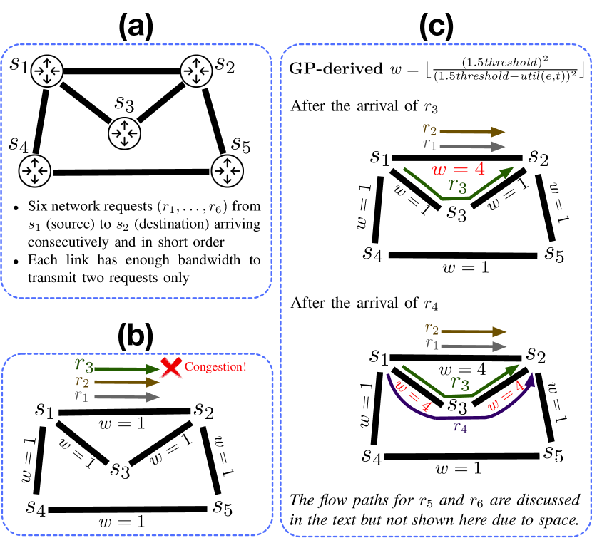
Figure 1. (a) A simple network alongside the description of network requests; (b) Output of a baseline data-forwarding algorithm; and (c) Output of data-forwarding after adaptation by our approach using genetic programming.

Optimization by re-routing flow paths has a major drawback. While optimizing at the level of individual flow paths may solve the currently observed congestion, doing so does not improve the logic of OSPF and thus does not contribute to congestion avoidance in the future. For instance, in Figure 1(b), the arrival of $r_{3}$ will cause congestion. Re-routing $r_{3}$ over $s_{1}\rightarrow s_{3}\rightarrow s_{2}$ will resolve this congestion. But, upon the arrival of $r_{4}$, OSPF will yet again select the flow path $s_{1}\rightarrow s_{2}$ for $r_{4}$ (since this is the shortest path between $s_{1}$ and $s_{2}$) just to find the $s_{1}\rightarrow s_{2}$ link congested again. This in turn necessitates the self-adaptation planning step to be invoked for $r_{4}$ as well. In a similar vein, the arrival of $r_{5}$ and $r_{6}$ will cause congestion, prompting further calls to self-adaptation planning.

Our proposal is that, instead of optimizing flow paths, one should optimize the logic of OSPF whenever a congestion is detected. In this paper, we optimize and update the link-weight formula that OSPF uses. The hypothesis here is that an optimized link-weight formula not only can resolve the existing congestion, but can simultaneously also make OSPF more intelligent towards congestion avoidance in the future, thus reducing the number of times that the self-adaptation planning step has to be invoked. Below, we illustrate our approach using the example of Figure 1.

We use genetic programming (GP) for self-adaptation planning, whereby we dynamically learn link-weight functions that not only help resolve an existing congestion but also help steer clear of future ones. Initially, and for requests $r_{1}$ and $r_{2}$, our approach does exactly as the standard OSPF would do, since there is no congestion. Upon the arrival of $r_{3}$ and the detection of congestion, i.e., the situation in Figure 1(b), our self-adaptation approach kicks in and automatically computes a link-weight formula such as the following: $\lfloor\frac{(1.5\mathit{threshold)^{2}}}{(1.5\mathit{threshold}-\mathit{util}(e,t))^{2}}\rfloor$. In this formula, $\mathit{util}(e,t)$ is the utilization percentage of link $e$ at time $t$, and $\mathit{threshold}$ is a constant parameter describing the utilization threshold above which the network is considered to be congested. In our example, $\mathit{threshold}=0.8$, and for each link, $\mathit{util}(e,t)$ is 0.3 if one flow passes through $e$, and is 0.6 if two flows pass through $e$. Given that $r_{1}$ and $r_{2}$ are already routed through $s_{1}\rightarrow s_{2}$, the weight of $s_{1}\rightarrow s_{2}$ computed by this formula becomes $w=4$; see Figure 1(c) after $r_{3}$’s arrival. As a result, OSPF selects path $s_{1}\rightarrow s_{3}\rightarrow s_{2}$ for $r_{3}$ which successfully resolves the current congestion observed in Figure 1(b). This, however, does not increase the weights for $s_{1}\rightarrow s_{3}$ and $s_{3}\rightarrow s_{2}$, since these links are utilized at $30$%, and their weights remain at 1. Once $r_{4}$ arrives, OSPF directs $r_{4}$ to $s_{1}\rightarrow s_{3}\rightarrow s_{2}$ as it is the shortest weighted path between $s_{1}$ and $s_{4}$. This will not cause any congestion, but the weights for $s_{1}\rightarrow s_{3}$ and $s_{3}\rightarrow s_{2}$ increase to $w=4$ since these links are now utilized at $60$%. Finally, OSPF will direct the last two requests $r_{5}$ and $r_{6}$ to the longer path $s_{1}\rightarrow s_{4}\rightarrow s_{5}\rightarrow s_{2}$, since, now, this path is the shortest weighted path between $s_{1}$ and $s_{2}$.

As shown above, using our GP-learned link-weight formula, OSPF is now able to manage flow paths without causing any congestion and without having to re-invoke the self-adaptation planning step beyond the single invocation after the arrival of $r_{3}$.

We note that there are several techniques that modify network parameters at runtime to resolve congestion in SDN (e.g., (Ghobadi et al., 2012; Priyadarsini et al., 2019)). These techniques, however, rely on pre-defined rules. For example, to make OSPF – discussed above – adaptive, a typical approach is to define a network-weight function (Rétvári et al., 2009). This function can involve parameters that change at runtime and based on the state of the network. However, the structure of the function is fixed. Consequently, the function may not be suitable for all networks with different characteristics and inputs. To address this limitation, we use GP to learn and evolve the function structure instead of relying on a fixed, manually crafted function. In Section 4, we compare our GP-based approach with OSPF configured using an optimized weight function suggested by Cisco standards (Coltun et al., 2008; Cis, 2005). As we show there, OSPF’s optimized weight function cannot address the congestion caused by the network-request bursts in our industrial case study.

In this paper, we focus on situations where congestion can be resolved by re-routing – in other words, when the network topology is such that alternative flow paths can be created for some requests. Given our focus, OSPF is a natural comparison baseline, noting that, in OSPF, congestion is resolved by re-routing. When alternative flow paths do not exist, congestion resolution can be addressed only via traffic shaping (Ghobadi et al., 2012), i.e., via modifying the network traffic. Our approach does not alter the network traffic. We therefore do not compare against congestion-resolution baselines that use traffic shaping.

3. Self-Adaptation Control Loop

Our approach leverages MAPE-K (Kephart and Chess, 2003; Moreno et al., 2015)– the well-known self-adaptation control-loop shown in Figure 2. The loop has four main steps: monitoring the system and its environment, analyzing the information collected from the system and its environment and deciding if adaptation is needed, planning on how to adapt, and executing the adaptation by applying it to the system.

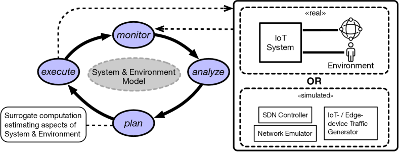
Figure 2. The MAPE-K (Kephart and Chess, 2003) self-adaptation control feedback-loop. The loop may interact with a real or simulated system. The plan step uses surrogates to estimate dynamic aspects of the system or the environment.

Our self-adaptation loop is an add-on to the programmable control layer of the SDN architecture. In an SDN, the control layer has a global view of the entire network and can dynamically modify the network at runtime. The routing logic of an SDN is centralized, decoupled from data and network hardware, and expressed using software code at the control layer. Given the separation of control logic from data planes and forwarding hardware, changing link weights can be programmed at the control layer in a way that the changes do not affect the existing network flows and instead are used only for routing new flows (Apostolopoulos et al., 1999). Dynamically modifying link weights therefore does not jeopardize network stability.

In our work, the self-adaptation loop interacts with a simulator instead of a real system. Using a simulator rather than an actual system is a common approach when designing and evaluating self-adaption techniques. This is because using the actual system for this purpose is time-consuming and expensive and may further cause system wear and damage (Iftikhar et al., 2017; Sotiropoulos et al., 2017). In addition, simulators are highly configurable and can imitate a variety of system configurations. Evaluating self-adaptation techniques using simulators enables us to cover a multitude of systems rather than one fixed setup (Borg et al., 2021; Menghi et al., 2019).

As shown on the right side of Figure 2, our simulator combines three components: An SDN controller capturing the software-defined controller of a network system (Berde et al., 2014); a network emulator that simulates the network infrastructure including links, nodes and their properties (Lantz et al., 2010); and a traffic generator (Botta et al., 2012) that emulates different types of requests generated by IoT devices and sensors.

We augment with GP the planning step of the self-adaptation loop. In order for GP to assess the fitness of candidate solutions, i.e., candidate link-weight functions, the system should be simulated for each candidate solution. This cannot be done using the simulator we use to replace the real system and its environment, since this simulator is real-time (wall-clock-time) and requires a few seconds to compute the behaviour of a network for each candidate weight-link formula. Our GP algorithm, when invoked, needs to explore several candidate formulas. To do so efficiently, we use surrogate computations that approximate the fitness values (Nejati, 2021; Menghi et al., 2020; Matinnejad et al., 2015). Specifically, as we detail in Section 3.2, our GP algorithm computes the fitness for each candidate solution using a snapshot of the system and its environment from the simulator, assuming that the system does not change during a small time period (expected to be less than one second, as we explain in Section 3.2).

Figure 3 shows a domain model consisting of two packages: One package, discussed in Section 3.1, captures the main elements of an SDN and its environment, and the other, discussed in Section 3.2, specifies the self-adaptation control loop that we develop.

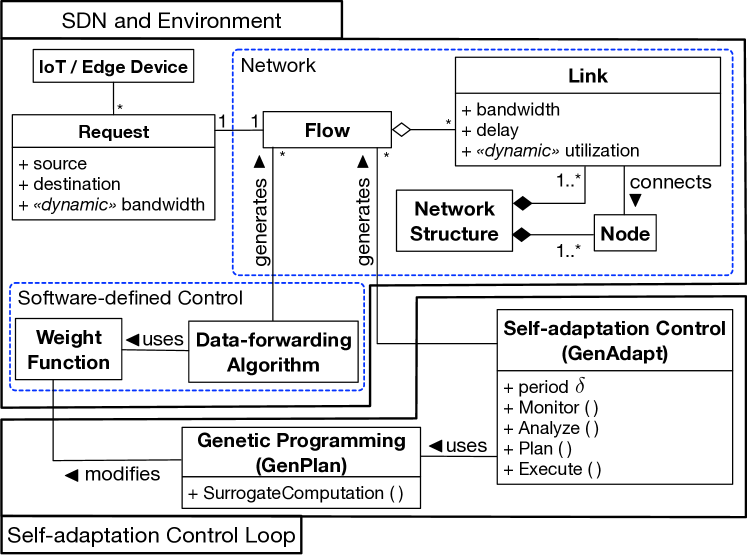
Figure 3. Domain model for self-adaptive SDN.

3.1. Domain Model for Self-adaptive SDN

The SDN and Environment package captures the static structure of a network as well as its dynamic behaviour over time. The environment of an SDN is comprised of IoT and edge devices which are connected to the network and which generate data-transmission requests (requests, for short) that the network needs to fulfil.

Definition 3.1 (Data-transmission Request).

A data-transmission request $r$ specifies a data stream sent by a network node $s$ to a network node $t$. We denote the source node of $r$ by $r.s$ and the destination node of $r$ by $r.t$. Let $[0..T]$ be a time interval. We denote the (data) bandwidth of $r$ at time $t\in[0..T]$ by $r.d(t)$. The bandwidth is the amount of data transmitted from $r.s$ to $r.t$ over time. We measure bandwidth in megabits per second (Mbps). The request bandwidth may vary over time (marked as “dynamic” in Figure 3).

In Figure 3, the network part of an SDN is delineated with a dashed rectangle labelled Network and includes the Network Structure, Link, Node and Flow entities. Specifically, a network is a tuple $G=(V,E)$, where $V$ is a set of nodes, and $E\subseteq V\times V$ is a set of directed links between nodes. Note that each (undirected) link in Figure 1 represents two directed links. Network links have a nominal maximum bandwidth and maximum transmission delay assigned to them based on their physical features and types. The bandwidth of a link is the maximum capacity of the link for transmitting data per second, and the maximum delay specifies the maximum time it takes for data transmission over a link.

Definition 3.2 (Static Properties of a Link).

Let $G=(V,E)$ be a network structure. Each link $e\in E$ has a bandwidth $bw(e)$ and a nominal delay $dl(e)$. We denote by $\mathit{StaticProp}(e)$ the tuple $(bw(e),dl(e))$, indicating the static properties of $e$.

As discussed in Section 2, a network handles requests by identifying a directed path (or a flow) in the network to transmit them. Upon the arrival of each request $r$, a network flow (path) $f$ is established to transmit the data stream of $r$ from the requested source $r.s$ to the requested destination $r.t$. Each flow $f$ is a directed path of links that connects $r.s$ to $r.t$. As shown in Figure 3, one flow is created per request. The bandwidth of each flow is equal to that of its corresponding request. Since requests have dynamic bandwidths (Definition 3.1), flows have dynamic bandwidths too. We define the throughput of link $e$ at time $t$, denoted by $\mathit{throughput}(e,t)$, as the total of the bandwidths of the flows going through $e$ at time $t$.

Definition 3.3 (Dynamic Utilization of a Link).

Let $G=(V,E)$ be a network, and let $[0..T]$ be a time interval. At each time $t\in[0..T]$, each network link $e\in E$ has a utilization $\mathit{util}(e,t)$ which is computed as follows: $\mathit{util}(e,t)=\mathit{throughput}(e,t)/\mathit{bw}(e)$.

The software-defined control entities in Figure 3 include Weight Function and Data-forwarding Algorithm. Data-forwarding algorithms are event-driven and handle requests upon arrival. As discussed in Section 2, data forwarding typically generates flows based on shortest weighted paths between the source and the destination of a request. Thanks to the SDN architecture, link weights are programmable and can be computed by a weight function that accounts for both the dynamic and the static properties of networks. For example, the GP-derived link-weight function in Figure 1 (c) uses the dynamic link utilization $\mathit{util}(e,t)$ and the static parameter $\mathit{threshold}$ to compute link weights.

3.2. Generative Self-adaptation

In this section, we describe GenAdapt, our self-adaptation control loop, and GenPlan, the genetic algorithm used in the planning step of GenAdapt. As discussed earlier, self-adaptation control has four main steps; these are specified as methods in the self-adaptation control entity in Figure 3. GenAdapt, i.e., our self-adaptation loop, runs in parallel with the data-forwarding algorithm. In contrast to the data-forwarding algorithm which is event-driven, GenAdapt is executed periodically with a period $\delta$, indicated as an attribute of GenAdapt in Figure 3. The self-adaptation loop periodically monitors the network for congestion as the environment changes, e.g., due to the arrival of new requests. There is a trade-off between the execution time of GenAdapt and the period $\delta$. In particular, $\delta$ should be small enough so that GenAdapt is executed frequently to detect and handle congestion promptly. At the same time, $\delta$ should be large enough so that frequent executions of GenAdapt do not interfere with other SDN algorithms and applications (Shin et al., 2020).

⬇

1Algorithm GenAdapt

2Input G : Network structure

3Input $\cup_{e\in E}$StaticProp($e$): Static properties of links

4Input BestSol: Best Solutions from the previous round

5Output F: Optimized flows

6Output W: Optimized weight function

7

8for every time step $i$ $\in\{1,\ldots,n\}$ do

9  F_i, $\cup_{e\in E}$util($e$, $i\cdot\delta$) $\leftarrow$ Monitor() //Dynamic data from SDN Sim

10  maxUtil = $\mathit{Max}\{\mbox{util}(e,i\cdot\delta)\}_{e\in E}$

11  if maxUtil $>$ $\mathit{threshold}$ then

12    F, W $\leftarrow$ GenPlan(G, $\cup_{e\in E}$StaticProp($e$), F_i, BestSol)

13    Apply F and W to the SDN data-forwarding algorithm

14  $\mathbf{end}$

15$\mathbf{end}$

Figure 4. Self-adaptation loop to resolve congestion by learning a new weight function for SDN data-forwarding.

GenAdapt, shown in Figure 4, executes at every time step $i{\cdot}\delta$ ($i=0,1,\ldots$). The monitor step (line 10) fetches the set $F_{i}$ of flows at time $i\cdot\delta$ and the utilization $\mathit{util}(e,i\cdot\delta)$ of every link $e$ at $i\cdot\delta$. The analyze step (lines 11-12) determines whether the network is congested, i.e., whether adaptation is needed. A network is congested if there is a link $e\in E$ which is utilized above a certain threshold (Lin et al., 2016; Akyildiz et al., 2014). To detect congestion, the maximum utilization of all the links is compared with $\mathit{threshold}$, which is a fixed parameter of the SDN.

If the network is congested, GenAdapt calls GenPlan (line 13). GenPlan, shown in Figure 5, is our GP algorithm which we discuss momentarily. The output of GenPlan is a new link-weight function as well as a modified set of flows where a minimal number of flows have been re-routed. The new flows and the optimized link-weight function are then applied to the SDN under analysis (line 14). Note that the only change that needs to be done to the network is re-routing a typically small number of flows to eliminate congestion.

GenPlan (Figure 5) generates link-weight functions that optimize a fitness function characterizing the desired network-flow properties. The link-weight functions are specified in terms of static link properties ($\mathit{bw}(e)$ and $\mathit{dl}(e)$), dynamic link utilization ($\mathit{util}(e,t)$) and utilization threshold. Note that GenPlan always reuses in its initial population half of the best solutions (candidate weight functions) generated by its previous invocation and stored in a variable named BestSol. Reusing as bootstrap some of the best solutions from the previous round ensures continuity and incrementality in learning the weight functions across multiple rounds of self-adaptation.

GenPlan starts by selecting a number of flows, BadFlows, from a congested set of flows, OldFlows, using the FindFlowsCausingCongestion algorithm shown in Figure 6. BadFlows are the flows that should be re-routed to resolve congestion. Following the standard steps of GP, GenPlan creates an initial population $P_{0}$ (line 14) containing a set of possible weight functions (individuals). For every individual $\omega\in P_{0}$, we call ComputeSurrogate, shown in Figure 7, to re-route the flows in BadFlows when $\omega$ is used to compute weights of the network links (line 19 of GenPlan). Specifically, for each $\omega$, ComputeSurrogate generates the set NewFlows which includes (1) the flows corresponding to those in BadFlows, but re-routed based on $\omega$; and (2) the original flows that did not cause congestion (i.e., OldFlows$\setminus$BadFlows). The set NewFlows is needed to compute the fitness value for $\omega$ (line 21). The fitness function aims to determine how close an individual is to resolving congestion. Our fitness function combines three criteria as we elaborate momentarily. GenPlan evolves the population by breeding and generating a new offspring population (line 17). The breeding and evaluation steps are repeated until a stop condition is satisfied. Then, GenPlan returns the link-weight function with the lowest fitness (BestW) and its corresponding flows (line 28).

The ComputeSurrogate algorithm (Figure 7), which is called by GenPlan, estimates the flows for each candidate weight function $\omega$, assuming that the flow bandwidths obtained at the monitoring step are constant over the duration of $\delta$. ComputeSurrogate first updates the utilization and weight values for each link, assuming that BadFlows are absent (lines 9-12). The new weights are then used to re-route each flow $f$ in BadFlows by identifying a flow $f^{\prime}$ as the new shortest path (line 14). After creating each new flow $f^{\prime}$, the utilization and weight values for each link on $f^{\prime}$ are updated (lines 15-18). Note that, because of the assumption that flow bandwidths remain fixed during $\delta$, the utilization-per-link $util(e)$ in ComputeSurrogate is not indexed by time.

⬇

1Algorithm GenPlan

2Input G: Network structure

3Input $\cup_{e\in E}$StaticProp($e$): Static properties of links

4Input OldFlows: Current network flows

5Input BestSol: Best Solutions from the previous round

6Output W: New weight function

7Output NewFlows: New network flows

8

9t = 0;

10BadFlows = FindFlowsCausingCongestion(OldFlows, G);

11Flows = OldFlows $\setminus$ BadFlows

12while not(stop_condition) do

13  if (t == 0)

14    P₀ = InitialPopOfWeightFormulas() $\cup$ BestSol

15    OffSprings = P₀

16  else

17    OffSprings = Breed(P_t)

18  $\mathbf{end}$

19  for $\omega\in$ OffSprings do

20    NewFlows = ComputeSurrogate(Flows, BadFlows, G, $\omega$)

21    $\omega$.Fit = Evaluate (G, NewFlows, OldFlows)

22  $\mathbf{end}$

23  P_t+1 = OffSprings

24  t = t + 1

25$\mathbf{end}$

26BestW = BestSolution(P₀, $\ldots$, P_t)

27bestFlows = ComputeSurrogate(Flows, BadFlows, G, BestW)

28return BestW, bestFlows

Figure 5. Generating a new link-weight function and a congestion-free set of flows using Genetic Programming.

Following standard practice for expressing meta-heuristic search problems (Harman et al., 2010), we define the representation, the fitness function, and the genetic operators underlying GenPlan.

Representation of the Individuals. An individual represents some weight function induced by the following grammar rule:

exp ::= exp ($+\mid-\mid*\mid/$) exp $|$ const $|$ StaticProp $|$ DynamicVar $|$ param

In the above, the symbol $\mid$ separates alternatives, const is an ephemeral random constant generator (Veenhuis, 2013), StaticProp are static link properties (Definition 3.2), DynamicVar is the link utilization (Definition 3.3), and param is some network parameter. The formula in Figure 1(c) can be generated by this grammar rule and is thus an example individual in GenPlan. Note that the SDN data-forwarding algorithm assumes that link values are integers. The $\lfloor\rfloor$ used in the formula of Figure 1(c) rounds down the output to an integer. Otherwise, $\lfloor\rfloor$ is not part of the weight formulas.

Each individual is constructed and manipulated as a parse tree. For example, the figure to the right shows the parse tree corresponding to $\frac{th^{2}}{(th-u)^{2}}$ where u is a shorthand for $util(e,t)$ and th is a shorthand for threshold. The initial population of GenPlan is generated by randomly building parse trees using the grow method (Poli et al., 2008) (i.e., the root and inner nodes are labelled by the mathematical operations, and the leaves are labelled by variables, constants or parameters specified in the grammar). As discussed earlier when GenPlan is called for the first time, the initial population is generated randomly. For subsequent calls to GenPlan, half of the initial population is generated and the other half is reused from the best elements in the last population generated by the previous invocation of GenPlan.

⬇

1Algorithm FindFlowsCausingCongestion

2Input G: Network structure

3Input Flows: Current flows

4Output BadFlows: A subset of Flows causing congestion

5

6BadFlows = $\emptyset$

7while G is congested do

8  Let $e$ be the most congested link

9  Let $f\in$ Flows such that $e\in f$ // selected randomly

10  BadFlows = BadFlows$\cup\{f\}$

11  Flows = Flows$\setminus\{f\}$

12$\mathbf{end}$

13return BadFlows

Figure 6. Selecting a subset of flows whose removal will resolve congestion.

⬇

1Algorithm ComputeSurrogate

2Input G: Network structure

3Input Flows: Current congestion-free set of flows

4Input BadFlows: Flows that have to be re-routed

5Input $\omega$: Candidate weight function

6Output NewFlows: BadFlows re-routed using $\omega$

7

8NewFlows $=\emptyset$

9for $e\in E$ do

10  util($e$) $\leftarrow$ sum of the bandwidths of $f\in$ Flows s.t. $e\in f$

11  Compute weight for $e$ using $\omega$

12$\mathbf{end}$

13for $f\in$ BadFlows do

14  $f^{\prime}$ $\leftarrow$ shortest weighted path from source to destination of $f$

15  for $e\in f^{\prime}$ do

16    util($e$) = util($e$) + bandwidth of $f^{\prime}$

17    update the weight of $e$ using $\omega$

18  $\mathbf{end}$

19  NewFlows = NewFlows$\cup\{f^{\prime}\}$

20$\mathbf{end}$

21return NewFlows $\cup$ Flows

Figure 7. Re-routing congested flows (BadFlows) by computing shortest paths based on a candidate weight function ($\omega$).

Fitness Function. Our fitness function is hybrid and combines the following three metrics: (1) Maximum link utilization across all the network links ($\mathit{Fit1}$). For each individual weight function $\omega$, GenPlan computes the set NewFlows of flows based on link weights generated by $\omega$. The $\mathit{Fit1}$ metric computes the utilization value of the most utilized network link, considering the flows in NewFlows. If $\mathit{Fit1}$ is higher than the threshold, then the network is congested. Hence, we are interested in individuals whose $\mathit{Fit1}$ is less than the threshold. (2) The cost of re-routing network flows measured as the number of link updates, i.e., insertions and deletions, required to reconfigure the network flows ($\mathit{Fit2}$). In GenPlan, OldFlows is the current set of congested flows, and as mentioned above, NewFlows is the set of flows computed for each individual $\omega$. We compute $\mathit{Fit2}$ as the edit distance between each pair of flows $f\in$ OldFlows and $f^{\prime}\in$ NewFlows such that $f$ and $f^{\prime}$ are both related to the same request. Specifically, the distance between two flows $f$ and $f^{\prime}$ is measured as the longest common subsequence (LCS) distance of two paths (Cormen et al., 2009) by counting the number of link insertions and link deletions required to transform $f$ into $f^{\prime}$. We note that this metric has previously been used as a proxy for the reconfiguration cost of network flows (Shin et al., 2020). (3) The total data transmission delay generated by the new flows ($\mathit{Fit3}$). The $\mathit{Fit3}$ metric is computed as the sum of all the delay values, i.e., $\mathit{dl(e)}$, of the links that are utilized by the new flows (i.e., the NewFlow set). The larger this value, the higher the overall transmission delay induced by NewFlows. The last metric allows us to penalize candidates that generate longer flows compared to those that generate shorter ones.

The $\mathit{Fit1}$, $\mathit{Fit2}$ and $\mathit{Fit3}$ metrics have different units of measure and ranges. Thus, before combining them, we normalize them using the well-known rational function $\bar{x}=x/(x+1)$. This function provides good guidance to the search for minimization problems compared to other alternatives.

Among the three metrics, lowering $\mathit{Fit1}$ below the congestion threshold takes priority; if a candidate solution is unable to resolve congestion, then we are not interested in the other two metrics. Once $\mathit{Fit1}$ is below the threshold, we do not want to lower $\mathit{Fit1}$ any further, since we want the network optimally utilized but not congested. Instead, we are interested in lowering the cost and delay metrics. We denote the normalized forms of our three metrics by $\overline{\mathit{Fit1}}$, $\overline{\mathit{Fit2}}$ and $\overline{\mathit{Fit3}}$, respectively, and define the following overall fitness function to combine the three:

$\begin{array}[]{l}Fit=\begin{cases}\overline{\mathit{Fit1}}+2&\text{(1) If $\mathit{Fit1}\geq\mathit{threshold}$}\\ \overline{\mathit{Fit2}}+\mathit{\overline{Fit3}}&\text{(2) If $\mathit{Fit1}<\mathit{threshold}$}\\ \end{cases}\end{array}$

Given a candidate weight function $\omega$, evaluating $\mathit{Fit}(\omega)$ always yields a value in $[0..3]$: $\mathit{Fit}(\omega)\geq 2$ indicates that $\omega$ is not able to resolve congestion; and $\mathit{Fit}(\omega)<2$ indicates that $\omega$ can resolve congestion, and its fitness determines how well $\omega$ is doing in reducing cost and delay. Note that in our fitness function defined above, cost and delay are equally important; we do not prioritize either one. If desired, one can modify the above function by adding coefficients to $\overline{\mathit{Fit2}}$ and $\overline{\mathit{Fit3}}$ to prioritize cost over delay or vice versa.

Genetic Operators. We use one-point crossover (Poli and Langdon, 1998). It randomly selects two parent individuals. It then randomly selects one sub-tree in each parent, and swaps the selected sub-trees resulting in two children. For the mutation operator, we use one-point mutation (Poli and B. Langdon, 1998) that mutates a child individual by randomly selecting one sub-tree and replacing it with a randomly generated tree, which is generated using the initialization procedure. For the parent selection operator, we use tournament selection (Luke, 2013).

4. Empirical Evaluation

In this section, we investigate the following research questions (RQs) using open-source synthetic and industrial IoT networks. To answer RQ1, we use the industrial network and ten synthetic networks. To answer RQ2, we use eight more synthetic networks alongside two of the synthetic networks from RQ1. In total, our evaluation involves one industrial network and 18 synthetic ones.

RQ1 (Effectiveness) How effective is GenAdapt in modifying the logic of the SDN data-forwarding algorithm to avoid future congestions? The main novelty of GenAdapt is in attempting to adapt the logic of SDN data forwarding (i.e., the link-weight functions) instead of adapting its output (i.e., the individual flow paths). Through RQ1, we compare GenAdapt with two baseline techniques: (i) an approach, named DICES (Shin et al., 2020), which, similar to GenAdapt, uses MAPE-K self-adaptation, but optimizes individual flow paths; and (ii) OSPF configured using a standard heuristic for setting optimized link weights (Coltun et al., 2008; Cis, 2005). By comparing GenAdapt with these baselines, we investigate whether GenAdapt, when called to resolve an existing congestion, is able to reduce the number of occurrences of congestion in the future, without incurring additional overhead.

RQ2 (Scalability): Can GenAdapt resolve congestion efficiently as the size of the network and the number of requests increase? To assess scalability, we evaluate the execution time of GenAdapt as the size of the network and the number of requests increase.

Implementation and Availability. We implemented GenAdapt using ECJ (version 27) (Scott and Luke, 2019) and the open-source version of DICES (Shin et al., 2020), which implements a self-adaptive control loop over the Open Network Operating System (ONOS) (Berde et al., 2014) – the SDN controller that we employ in our work. Similar to DICES, our simulator consists of three open-source tools: (i) ONOS (Berde et al., 2014) as the “SDN Controller” (see Figure 2), (ii) Mininet (Lantz et al., 2010) as the “Network Emulator”, and (iii) Distributed Internet Traffic Generator (D-ITG) (Botta et al., 2012) as the “IoT-/Edge-device Traffic Generator”. Our simulator is memory-intensive and runs on two Linux virtual machines (VMs), but GenAdapt by itself does not require special considerations for memory or CPU power. All experiments were performed on a machine with a 2.5 GHz Intel Core i7 CPU and 32 GB of memory. Our implementation and all experimental material are available online (app, 2021).

4.1. RQ1 – Effectiveness

Before answering RQ1, we present the baselines, the study subjects, the configuration of GenAadapt and the setup of our experiments.

Baselines. Our first baseline, DICES, is from the SEAMS literature. Similar to GenAadapt, DICES is self-adaptive, but unlike GenAadapt, it uses a genetic algorithm to modify the individual flows generated by the SDN data-forwarding algorithm. The second baseline is OSPF (Coltun et al., 2008; Cis, 2005) configured by setting the link weights to be inversely proportional to the bandwidths of the links as suggested by Cisco (Cis, 2005). The OSPF heuristic link weights are meant to induce optimal flows that eliminate or minimize the likelihood of congestion. OSPF is widely used in real-world systems (Fortz and Thorup, 2002) and as a baseline in the literature (Poularakis et al., 2019; Amin et al., 2018; Bianco et al., 2017; Rego et al., 2017; Caria et al., 2015; Bianco et al., 2015; Agarwal et al., 2013).

Study Subjects. For RQ1, we use: (1) ten synthetic networks, and (2) an industrial SDN-based IoT network published in earlier work (Shin et al., 2020). For the synthetic networks, we consider two network topologies: (i) complete graphs, and (ii) multiple non-overlapping paths between node pairs. The network in Figure 1 is an example of the latter topology, where $s_{1}$ and $s_{2}$ are connected by three non-overlapping paths. Since our approach works by changing flow paths, we naturally focus our evaluation on topologies with multiple paths from a source to a destination, thus excluding topologies where adaptation through re-routing is not possible. The topologies that we experiment with, i.e., (i) and (ii) above, are the two extreme ends of the spectrum in terms of path overlaps between node pairs: In the first case, we have complete graphs where there are as many overlapping paths as can be between node pairs; and, in the second case, we have no overlapping paths at all. We consider four complete graphs – referred to as FULL hereafter – with five, six, seven and ten nodes, and consider two multiple-non-overlapping path graphs – referred to as MNP hereafter – with five and eight nodes. More precisely, one MNP graph has five nodes connecting the designated source and destination with three non-overlapping paths (Figure 1); the other has eight nodes doing the same with four (non-overlapping) paths. Following the suggested parameter values in the existing literature for such experiments (Shin et al., 2020), we set the static properties of the links, namely bandwidth and delay, to 100Mbps and 25ms, respectively.

To instigate changes in the SDN environment, we generate data requests over time and not at once. We space the requests $10$s apart to ensure that all the requests are properly generated and that the network has some time to stabilize, i.e., we send requests at $0$s, $10$s, $20$s, $30$s, and so on. For each FULL network, we fix a source and a destination node, and generate either three or four requests every $10$s. For each MNP network, we generate every $10$s two requests between the end-nodes connected by multiple paths. The reason why we generate fewer requests in the MNP networks is because there are fewer paths compared to the FULL networks. For a given network (FULL or MNP), the generated requests have the same bandwidth. The request bandwidth for each network is selected such that some congestion is created starting from $10$s. The request bandwidths are provided online (app, 2021). We denote our synthetic networks by FULL($x$, $y$) and MNP($x$, $y$), where $x$ is the number of nodes and $y$ is the number of requests generated every $10$s. The ten synthetic network that we use in RQ1 are four FULL networks, once with three requests and once with four requests generated every $10$s, and two MNP networks with two requests generated every $10$s.

Our industrial subject is an emergency management system (EMS) from previous work (Shin et al., 2020). EMS represents a real-world application of SDN in a complex IoT system. This subject contains seven switches and 30 links with different values for the links’ static properties. The EMS subject includes a traffic profile characterizing anticipated traffic at the time of a natural disaster (e.g., flood), leading to congestion in the network of the monitoring system. In particular, the network is used for transmitting 28 requests capturing different data stream types such as audio, video and sensor and map data. The static properties of the network links and the data-request sizes are available online (app, 2021) .

Experiments and metrics. RQ1 has two goals: (G1) determine whether, by properly modifying the link-weight function, GenAdapt is able to reduce the number of times congestion happens, and (G2) determine whether GenAdapt can respond quickly enough so that prolonged periods of congestion can be avoided.

The synthetic subjects are best used for achieving G1, since the requests in these subjects are generated with time gaps as opposed to all at once, which is the case in EMS (industry subject). This characteristic of the synthetic subjects creates the potential for congestion to occur multiple times, in turn allowing us to achieve G1. For G1, we compare GenAdapt with DICES; comparison with the OSPF baseline does not apply, since OSPF’s heuristic cannot avoid congestion for our synthetic subjects, and neither can it resolve congestion. To compare GenAdapt with DICES, we keep track of how many times congestion occurs during our simulation, the execution time of each technique to resolve each congestion occurrence, and the total time during which the network is in a congested state. In addition, we measure packet loss, which is a standard metric for detecting congestion in network systems. Packet loss is measured as the number of dropped packets divided by the total number of packets in transit across the entire network during simulation. The simulation time for each synthetic subject was set to end $10$s after the generation of the last request. Recall that, in our synthetic subjects, the requests are sent at intervals of $10$s and as long as the number of paths in the underlying network is sufficient to fulfill the incoming the requests.

To achieve G2, we use EMS in order to compare GenAdapt with DICES and OSPF in terms of handling the congestion caused by requests arriving at once. Since DICES and GenAdapt are self-adaptive, they monitor EMS and attempt to resolve congestion when it occurs. In the case of OSPF, however, the heuristic link weights are meant to reduce the likelihood of congestion and packet loss. For this comparison, we report the total packet loss recorded by each of the three technique over a fixed simulation interval of $5$min, and also whether, or not, GenAdapt and DICES were able to resolve the congestion in EMS within the simulation time.

Configuring GenAdapt. Table 1 shows the configuration parameters used for GenAdapt. For the mutation and crossover rates, the maximum tree depth and the tournament size, we chose recommendations from either the GP literature (Poli et al., 2008; Luke and Panait, 2006) or ECJ’s documentation (Scott and Luke, 2019). We set $\delta$ to $1$s since this is the smallest monitoring period permitted by our simulator. We use the utilization threshold given in the literature (Shin et al., 2020; Akyildiz et al., 2014; Lin et al., 2016). Since the range for link-utilization values is [$0$% .. $100$%], we set the minimum and maximum of the constants in GP individuals to $0$ and $100$, respectively.

Table 1. Parameters of GenAdapt.

Mutation rate	0.1	Utilization threshold	$80$%
Crossover rate	0.7	Minimum of the constant in the GP grammar	0
Maximum depth of GP tree	5	Maximum of the constant in the GP grammar	100
Tournament size	7	Interval between invocations of GenAdapt ($\delta$)	$1$s
Population size	10

To determine the population size and the number of generations for GP, we note that, ideally, GenAdapt should not take longer than $\delta$ to execute. The execution time of GenAdapt is likely shorter when it is called in the first rounds of request generation than in the later rounds, since there are fewer flows in the early rounds of our synthetic subjects. Hence, using the fixed time limit of $1$s to stop GenAdapt is not optimal. Instead of using a time limit, we performed some preliminary experiments on our synthetic subjects to configure population size and the number of generations for the two topologies of FULL and MNP. For both topologies, we opt to use a small population size (i.e., $10$). As for the number of generations, for the FULL networks, we stop GenAdapt when the fitness function falls below two (i.e., when congestion is resolved but the solution is not necessarily optimized for delay and cost) or when 200 generations is reached. This will ensure that GenAdapt’s execution time does not exceed $1$s for our FULL networks. The MNP networks are, however, sparser and we are able to increase the number of generations while keeping the execution time below $1$s. Specifically, for MNP networks with five nodes, we use 300 generations; and, for the one with eight nodes we use 500 generations. For EMS, the topology is more similar to a full graph, and as such, we use the same configuration for EMS as that for FULL networks.

Results. As an example, Figure 8 shows the network utilization over time when GenAdapt and DICES are used to resolve congestion for the synthetic network MNP(8, 2). Two simultaneous network requests are sent at 0s, 10s, 20s and 30s, leading to congestion at 10s, 20s, and 30s. The network is congested when the utilization value is above 0.8 (i.e., the utilization threshold). Out of 30 runs for DICES, 18 runs record three congestion occurrences and 12 runs record four. In contrast, out of 30 runs for GenAdapt, six runs record only one congestion occurrence, 16 runs record two, seven runs record three, and only one run records four congestion occurrences. Note that three congestion occurrences at 10s, 20s, and 30s are visible in the figure. However, in the simulated environment, similar to the physical world, there are some small time gaps between the arrivals of the two requests generated each time, and in addition, there are small fluctuations in flow bandwidths over time. Hence, the monitoring step of GenAdapt or DICES may detect congestion twice (i.e., once per request arrival), instead of only once and after the arrival of both requests. In total, for the example in Figure 8, the average number of congestion occurrences is 2.1 with GenAdapt and 3.4 with DICES. In addition, with DICES, the average of the total time that the network remains congested is 7.6s, while with GenAdapt, this is reduced to 5.57s.

Figure 8. Comparing network utilization values over time obtained from 30 runs of DICES and GenAdapt for resolving congestion in an example synthetic subject: MNP(8,2).

Table 2. Statistical-test results comparing the average number of congestion occurrences, the duration of congestion, the execution-time and the packet-loss values obtained by 30 runs of GenAdapt versus DICES for our ten synthetic subjects.

FULL(5,3)

FULL(5,4)

FULL(6,3) – 40% of DICES runs failed

FULL(6,4) – 33.3% of DICES runs failed

FULL(7,3) – 66.6% of DICES runs failed

avg(G-D)∗

p-value

$\bf{\hat{A}_{12}}$

avg(G-D)

p-value

$\bf{\hat{A}_{12}}$

avg(G-D)

p-value

$\bf{\hat{A}_{12}}$

avg(G-D)

p-value

$\bf{\hat{A}_{12}}$

avg(G-D)

p-value

$\bf{\hat{A}_{12}}$

# Congestion

3.1 – 3.2

0.98

0.5(N)

3.8 – 4.4

0.193

0.59(S)

3.5 – 4.5

0.003

0.74(L)

3.8 – 5.4

5.39E-06

0.87(L)

4.1 – 6

9.70E-08

1(L)

Congestion Duration (s)

6.2 – 7.7

0.0919

0.62(S)

9.53 – 12

0.145

0.61(S)

7.93 – 12

1.69E-06

0.86(L)

10.03 – 14.47

5.98E-05

0.8(L)

8.03 – 16.63

1.35E-11

1(L)

Packet Loss (%)

32.1 – 32.33

0.001

0.75(L)

24.86 – 24.99

0.535

0.45(N)

24.94 – 31.73

7.96E-11

0.94(L)

28.4 – 31.64

1.53E-05

0.83(L)

16.6 – 19.7

0.145

0.61(S)

Exec Time (ms)

140.86 – 392.96

¡2.2E-16

0.98(L)

271.95 – 440.87

¡2.2E-16

0.87(L)

302.21 – 701.06

¡2.2E-16

0.9(L)

956.47 – 802.48

¡2.2E-16

0.85(L)

295.94 – 949.2

¡2.2E-16

0.97(L)

FULL(7,4)

FULL(10,3)

FULL(10,4) – 10% of DICES runs failed

MNP(5,2)

MNP(8,2)

avg(G-D)

p-value

$\bf{\hat{A}_{12}}$

avg(G-D)

p-value

$\bf{\hat{A}_{12}}$

avg(G-D)

p-value

$\bf{\hat{A}_{12}}$

avg(G-D)

p-value

$\bf{\hat{A}_{12}}$

avg(G-D)

p-value

$\bf{\hat{A}_{12}}$

# Congestion

2.9 – 3.1

0.063

0.59(S)

3.7 – 4

0.464

0.58(S)

4 – 5.9

9.21E-11

0.96(L)

1.8 – 2.2

0.002

0.68(M)

2.1 – 3.4

1.55E-08

0.9(L)

Congestion Duration (s)

5 – 5.97

0.0157

0.68(M)

7.5 – 8.47

0.029

0.65(S)

8.9 – 16.23

9.53E-11

0.98(L)

3.87 – 5.23

0.0029

0.71(M)

5.57 – 7.6

0.0002

0.77(L)

Packet Loss (%)

10.13 – 19.31

8.08E-07

0.87(L)

8.75 – 13.02

0.006

0.71(M)

30.17 – 34.41

1.61E-10

0.98(L)

32.39 – 32.65

0.004

0.72(M)

32.6 – 33.6

3.43E-06

0.85(L)

Exec Time (ms)

226.40 – 576.05

¡2.2E-16

0.99(L)

564.88 – 814.8

4.65E-16

0.81(L)

596.31 – 1365.28

¡2.2E-16

0.86(L)

381.07 – 469.13

0.099

0.59(S)

787.06 – 392.62

¡2.2E-16

0.08(L)

* The avg(G-D) column shows the average (avg) metrics for GenAdapt (G) versus those for DICES (D).

With the analysis for RQ1 intuitively explained over one subject, namely MNP(8,2), we now present the complete results for this RQ. Table 2 compares GenAdapt against DICES for our ten synthetic subjects (i.e., four FULL($n$, 3), four FULL ($n$, 4) and two MNP($n$, 2) where $n$ is the number of network nodes) by reporting the average number of congestion occurrences, the average total duration that the network is congested, the average execution time, and the average packet-loss values obtained by 30 runs of DICES and GenAdapt. For four subjects, some runs of DICES failed to resolve the last congestion within the simulation time. Specifically, for FULL(6,3), 12 runs; for FULL(6,4), 10 runs; for FULL(7,3), 20 runs; and for FULL(10,4), 3 runs of DICES failed to resolve congestion. For these subjects, the reported average number of congestion occurrences and execution times capture only the successful runs of DICES. In contrast, all runs of GenAdapt for all the subjects successfully resolved congestion within the simulation time.

We compare the results of Table 2 through statistical testing. We use the non-parametric pairwise Wilcoxon rank sum test (Capon, 1991) and the Vargha-Delaney’s $\hat{A}_{12}$ effect size (Vargha and Delaney, 2000). We first focus on the following three metrics: number of congestion occurrences, congestion duration, and packet loss. For fives subjects – MNP(8,2), MNP(5,2), FULL(10,4), FULL(6,4), and FULL(6,3) – the $p$-values for all the comparisons of the above three metrics are lower than $0.05$ and the $\hat{A}_{12}$ statistics show large or medium effect sizes, indicating that GenAdapt significantly improves DICES w.r.t. the three metrics on the five subjects. For the four other subjects – FULL(5, 3), FULL(7,3), FULL(7,4) and FULL(10, 3) – GenAdapt significantly improves DICES with large or medium effect sizes w.r.t. at least one of these three metrics. For all the subjects, the averages of these three metrics obtained by GenAdapt are better than those obtained by DICES, and there is no case where DICES performs better than GenAdapt w.r.t. any of these three metrics.

As for the execution time, a larger execution time, as long as it is not worsening the other three metrics, is not a weakness. For eight subjects, the average execution time of GenAdapt is significantly better than that of DICES and for two, it is the opposite. In those two cases, however, while GenAdapt is slower than DICES on average, it still significantly outperforms DICES w.r.t. the other three metrics.

Figure 9 shows the packet-loss values obtained by 30 runs of GenAdapt, DICES and OSPF applied to the industry subject (EMS). All 30 runs of GenAdapt and DICES could resolve the congestion in EMS within the simulation time. However, OSPF incurs high packet loss (avg. $36.5$%), since its heuristic link weights cannot prevent congestion in EMS. Both GenAdapt and DICES start with high packet loss, but since they can resolve congestion, packet loss drops quickly, yielding low averages over the duration of simulation. The differences between the packet-loss values of GenAdapt and DICES are neither statistically significant ($p$-value = 0.44) nor practically significant – a packet-loss difference of 0.4% is negligible in practice. The results of Figure 9 signify the need for runtime adaptation in EMS. Further, the results in both Table 2 and Figure 9 show that while GenAdapt can reduce congestion occurrences over time compared to DICES, doing so does not come at the cost of being less effective in resolving a one-off congestion in EMS caused by several requests arriving almost at once.

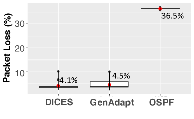
Figure 9. Comparing packet-loss values obtained by 30 runs of DICES, GenAdapt and OSPF.

The answer to RQ1 is that GenAdapt successfully resolves congestions in all the subjects. Compared to DICES, GenAdapt reduces the average number of congestions for six subjects with a high statistical significance, while DICES never outperforms GenAdapt in any of the congestion resolution metrics. Further, for our industry subject, GenAdapt significantly outperforms the standard SDN data-forwarding algorithm, OSPF, in reducing packet loss.

4.2. RQ2 – Scalability

To answer RQ2, we perform two sets of studies. In the first set, we increase the network size and in the second set – the number of requests. Specifically, first, we create ten synthetic networks with the FULL topology and having 5, 10, …, 50 nodes; and, for each network, we generate five requests with the same bandwidth at once to reach a total bandwidth of 150Mbps. Second, we create a five-node network with the FULL topology and execute ten different experiments by subsequently generating 5, 10, …, 50 requests at once such that for each experiment, the requests have the same bandwidth and the sum of the requests’ bandwidths is 150Mbps. For both experimental sets, we record the execution time of the configuration of GenAdapt used for the FULL topology as described in Section 4.1. Our experimental setup in RQ2 follows that used by DICES for scalability analysis. We focus on the FULL topology for scalability analysis because networks with this topology have considerably more links and pose a bigger challenge for self-adaptation planning, as evidenced by the failure of DICES over several networks with the FULL topology (see Table 2).

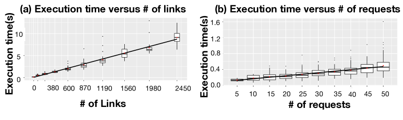
Figure 10. Execution times of GenAdapt versus (a) number of links and (b) number of requests.

Figure 10 shows the execution time of GenAdapt versus the number of network links (Figures 10(a)), and versus the number of requests (Figure 10(b)). For each network size and for each number of requests, GenAdapt is executed 30 times. For each diagram in Figures 10, we have fitted a linear regression line ($\mathit{time}=-0.019+0.0036\times\mathit{links}$ in Figure 10(a); and $\mathit{time}=0.087+0.0077\times\mathit{links}$ in Figure 10(b)). In both cases, we obtain a $p$-value of $<2.2e-16$, indicating that the models fit the data well.

The answer to RQ2 is that the execution time of GenAdapt is linear in the number of requests and in the size of the network.

4.3. Threats to Validity

Construct and external validity are the validity aspects most pertinent to our evaluation.

Construct validity. Our experiments are simulation-based; the extent to which the measurements obtained through simulation are reflective of the real world is therefore an important factor to consider. To this end, we note that the tools that our simulator builds on, i.e., ONOS and Mininet, are widely considered to be high-fidelity network simulators (Zhu et al., 2021; Azzouni et al., 2017; Berde et al., 2014; Bianco et al., 2017). While the high fidelity of our simulator provides confidence about our results, future experimentation with real IoT networks remains necessary.

External validity. We scoped our experiments to two network topologies only. As discussed in Section 4.1, the two topologies are the two extreme ends of the spectrum in terms of path overlaps between node pairs – the main determinant of complexity for GenAdapt. We expect that, for other topologies lending themselves to congestion resolution via re-routing, our approach will behave within the same range as seen in our experiments. To ensure adequate coverage, our evaluation examined 18 networks based on the two topologies considered. In addition, our evaluation included a real industrial IoT network with its own topology. The number, size and complexity of the networks in our experiments are comparable to those in the literature, e.g., (Shin et al., 2020; Azzouni et al., 2017; Liu et al., 2018; Zhu et al., 2021; Agarwal et al., 2013). A second consideration related to external validity is the tuning of our approach. The only parameter of our approach that requires tuning by the user is the number of generations of GenAdapt. As discussed in Section 4.1, tuning this parameter is straightforward based on the easily measurable objective of keeping the execution time of GenAdapt less than $\delta$ (i.e., the time interval between consecutive invocations of GenAdapt). In practice, engineers can use our simulator to tune this parameter for their specific network topology and traffic profile.

5. Related Work

We compare our approach with related work in software engineering for self-adaptive systems and in congestion control for SDN.

Self-adaptive systems. Engineering self-adaptive systems, including the principles underlying the construction, maintenance and evolution of such systems, have been studied from different angles and for different domains (Krupitzer et al., 2018; Coker et al., 2015; Bhuiyan et al., 2017; Anaya et al., 2014; Stein et al., 2016; Garlan et al., 2009; Cheng et al., 2013). Our work relates to dynamic adaptive search-based software engineering (Harman et al., 2012) which uses a blend of artificial intelligence (AI) and optimization to adapt system properties. Prior research in this field has used search algorithms for different purposes such as configuring properties of self-adaptive systems (Ramirez et al., 2009; Zoghi et al., 2016) and improving the design and architecture of such systems (Menascé et al., 2011; Andrade and de A. Macêdo, 2013; Ramirez and Cheng, 2010). The closest work to ours is DICES (Shin et al., 2020), which is used as a baseline for our experiments. Our approach, in contrast to DICES, is generative and aims to reduce the need for invoking adaptations over time.

Our work relates to AI-enabled adaptation (Quin et al., 2019; Gheibi et al., 2021). Among different AI methods, we use GP because of its flexibility to learn formulas that match our specific grammar for link-weight functions. To our knowledge, we are the first to apply GP for adapting IoT networks and reducing the need for frequent adaptations in this domain.

Congestion control in SDN. Network congestion resolution has been studied extensively (Mathis and Mahdavi, 1996; Alizadeh et al., 2010; He et al., 2016; Betzler et al., 2016). Some congestion resolution approaches work by adjusting data transmission rates (Betzler et al., 2016). Several others focus on traffic engineering to provide solutions for better traffic control, better traffic operation, and better traffic management, e.g., by multi-path routing (Han et al., 2015), creating a new routing technique (Mao et al., 2017), and flow-based routing (Amokrane et al., 2013). Our work is related to the research that utilizes the additional flexibility offered by the programmable control in the SDN architecture (Brandt et al., 2016; Hong et al., 2013; Chiang et al., 2018; Agarwal et al., 2013; Gay et al., 2017; Huang et al., 2016; Shin et al., 2020; Ghobadi et al., 2012). Within this line of research, congestion control is commonly cast as an optimization problem (Chiang et al., 2018), to be solved using local search (Gay et al., 2017) or linear programming (Agarwal et al., 2013). Some techniques (Ghobadi et al., 2012) adapt the network parameters at runtime using a pre-defined set of rules. In contrast to our work, none of these techniques evolve the rules in response to feedback from SDN monitoring.

6. Conclusion

We presented GenAdapt – an adaptive approach that uses genetic programming for resolving network congestion in SDN-based IoT networks. While existing self-adaptation research focuses on modifying a running system via producing individual and concrete elements, GenAdapt is generative and modifies the logic of the running system so that the system itself can generate the concrete elements without needing frequent adaptations. We used 18 synthetic and one industrial network to compare GenAdapt against two baseline techniques: DICES (Shin et al., 2020) and OSPF (Coltun et al., 2008; Cis, 2005). GenAdapt successfully resolved all congestion occurrences in our experimental networks, while DICES failed to do so in four of them. Further, compared to DICES, GenAdapt reduced the number of congestion occurrences and outperformed OSPF in reducing packet loss.

- (1)
- Cis (2005) 2005. Cisco. OSPF Design Guide. Documentation at https://www.cisco.com/c/en/us/support/docs/ip/open-shortest-path-first-ospf/7039-1.html.
- app (2021) 2021. GenAdapt. https://figshare.com/s/de6eb6e61816401b5c9e
- Agarwal et al. (2013) Sugam Agarwal, Murali S. Kodialam, and T. V. Lakshman. 2013. Traffic Engineering in Software Defined Networks. In Proceedings of the 2013 Annual IEEE International Conference on Computer Communications (INFOCOM’13). 2211–2219.
- Akyildiz et al. (2014) Ian F. Akyildiz, Ahyoung Lee, Pu Wang, Min Luo, and Wu Chou. 2014. A Roadmap for Traffic Engineering in SDN-OpenFlow Networks. Computer Networks 71 (2014), 1–30.
- Alizadeh et al. (2010) Mohammad Alizadeh, Albert G. Greenberg, David A. Maltz, Jitendra Padhye, Parveen Patel, Balaji Prabhakar, Sudipta Sengupta, and Murari Sridharan. 2010. Data Center TCP (DCTCP). In Proceedings of the 2010 ACM Conference on Special Interest Group on Data Communication (SIGCOMM’10). 63–74.
- Alrajeh et al. (2020) Dalal Alrajeh, Antoine Cailliau, and Axel van Lamsweerde. 2020. Adapting requirements models to varying environments. In ICSE ’20: 42nd International Conference on Software Engineering, Seoul, South Korea, 27 June - 19 July, 2020, Gregg Rothermel and Doo-Hwan Bae (Eds.). ACM, 50–61.
- Amin et al. (2018) Rashid Amin, Martin Reisslein, and Nadir Shah. 2018. Hybrid SDN Networks: A Survey of Existing Approaches. IEEE Communications Surveys and Tutorials 20, 4 (2018), 3259–3306.
- Amokrane et al. (2013) Ahmed Amokrane, Rami Langar, Raouf Boutaba, and Guy Pujolle. 2013. Online flow-based energy efficient management in Wireless Mesh Networks. In 2013 IEEE Global Communications Conference, GLOBECOM 2013, Atlanta, GA, USA, December 9-13, 2013. IEEE, 329–335.
- Anaya et al. (2014) Ivan Dario Paez Anaya, Viliam Simko, Johann Bourcier, Noël Plouzeau, and Jean-Marc Jézéquel. 2014. A Prediction-driven Adaptation Approach for Self-Adaptive Sensor Networks. In Proceedings of the 9th International Symposium on Software Engineering for Adaptive and Self-Managing Systems SEAMS’14. 145–154.
- Andrade and de A. Macêdo (2013) Sandro S. Andrade and Raimundo José de A. Macêdo. 2013. A Search-Based Approach for Architectural Design of Feedback Control Concerns in Self-Adaptive Systems. In Proceedings of the 7th IEEE International Conference on Self-Adaptive and Self-Organizing Systems (SASO’13). 61–70.
- Apostolopoulos et al. (1999) G. Apostolopoulos, S. Kamat, D. Williams, R. Guérin, A. Orda, and T. Przygienda. 1999. QoS Routing Mechanisms and OSPF Extensions. RFC 2676 (1999), 1–50.
- Azzouni et al. (2017) Abdelhadi Azzouni, Raouf Boutaba, and Guy Pujolle. 2017. NeuRoute: Predictive dynamic routing for software-defined networks. In 13th International Conference on Network and Service Management, CNSM 2017, Tokyo, Japan, November 26-30, 2017. IEEE Computer Society, 1–6.
- Berde et al. (2014) Pankaj Berde, Matteo Gerola, Jonathan Hart, Yuta Higuchi, Masayoshi Kobayashi, Toshio Koide, Bob Lantzand Brian O’Connor, Pavlin Radoslavov, William Snow, and Guru Parulkar. 2014. ONOS: Towards an Open, Distributed SDN OS. In Proceedings of the 3rd Workshop on Hot Topics in Software Defined Networking (HotSDN’14). 1–6.
- Betzler et al. (2016) August Betzler, Carles Gomez, Ilker Demirkol, and Josep Paradells. 2016. CoAP Congestion Control for the Internet of Things. IEEE Communications Magazine 54, 7 (2016), 154–160.
- Bhuiyan et al. (2017) Md Zakirul Alam Bhuiyan, Jie Wu, Guojun Wang, Tian Wang, and Mohammad Mehedi Hassan. 2017. e-Sampling: Event-Sensitive Autonomous Adaptive Sensing and Low-Cost Monitoring in Networked Sensing Systems. ACM Transactions on Autonomous and Adaptive Systems (TAAS) 12, 1 (2017), 1:1–1:29.
- Bianco et al. (2015) Andrea Bianco, Paolo Giaccone, Ahsan Mahmood, Mario Ullio, and Vinicio Vercellone. 2015. Evaluating the SDN control traffic in large ISP networks. In Proceedings of the 2015 IEEE International Conference on Communications (ICC’15). 5248–5253.
- Bianco et al. (2017) Andrea Bianco, Paolo Giaccone, Reza Mashayekhi, Mario Ullio, and Vinicio Vercellone. 2017. Scalability of ONOS reactive forwarding applications in ISP networks. Computer Communications 102 (2017), 130–138.
- Borg et al. (2021) Markus Borg, Raja Ben Abdessalem, Shiva Nejati, François-Xavier Jegeden, and Donghwan Shin. 2021. Digital Twins Are Not Monozygotic - Cross-Replicating ADAS Testing in Two Industry-Grade Automotive Simulators. In 14th IEEE Conference on Software Testing, Verification and Validation, ICST 2021. IEEE, 383–393.
- Botta et al. (2012) Alessio Botta, Alberto Dainotti, and Antonio Pescapè. 2012. A Tool for The Generation of Realistic Network Workload for Emerging Networking Scenarios. Computer Networks 56, 15 (2012), 3531–3547.
- Brandt et al. (2016) Sebastian Brandt, Klaus-Tycho Foerster, and Roger Wattenhofer. 2016. On Consistent Migration of Flows in SDNs. In Proceedings of the 2016 Annual IEEE International Conference on Computer Communications (INFOCOM’16). 1–9.
- Capon (1991) J. Anthony Capon. 1991. Elementary Statistics for the Social Sciences: Study Guide. Wadsworth Publishing Company, Belmont, CA, USA.
- Caria et al. (2015) Marcel Caria, Tamal Das, and Admela Jukan. 2015. Divide and conquer: Partitioning OSPF networks with SDN. In Proceedings of the 2015 IFIP/IEEE International Symposium on Integrated Network Management (IM’15). 467–474.
- Cheng et al. (2013) Betty H. C. Cheng, Andres J. Ramirez, and Philip K. McKinley. 2013. Harnessing evolutionary computation to enable dynamically adaptive systems to manage uncertainty. In 1st International Workshop on Combining Modelling and Search-Based Software Engineering, CMSBSE@ICSE 2013, San Francisco, CA, USA, May 20, 2013. IEEE Computer Society, 1–6.
- Chiang et al. (2018) Sheng-Hao Chiang, Jian-Jhih Kuo, Shan-Hsiang Shen, De-Nian Yang, and Wen-Tsuen Chen. 2018. Online Multicast Traffic Engineering for Software-Defined Networks. In Proceedings of the 2018 Annual IEEE International Conference on Computer Communications (INFOCOM’18). 414–422.
- Coker et al. (2015) Zack Coker, David Garlan, and Claire Le Goues. 2015. SASS: Self-adaptation Using Stochastic Search. In Proceedings of the 10th International Symposium on Software Engineering for Adaptive and Self-Managing Systems SEAMS’15. 168–174.
- Coltun et al. (2008) Rob Coltun, Dennis Ferguson, John Moy, and Acee Lindem. 2008. OSPF for IPv6. Internet Standard RFC 5340. Network Working Group.
- Cormen et al. (2009) Thomas H. Cormen, Charles E. Leiserson, Ronald L. Rivest, and Clifford Stein. 2009. Introduction to Algorithms (3rd ed.). The MIT Press.
- DeVries and Cheng (2017) Byron DeVries and Betty H. C. Cheng. 2017. Using Models at Run Time to Detect Incomplete and Inconsistent Requirements. In Proceedings of MODELS 2017 Satellite Events, Austin, TX, USA, September, 17, 2017 (CEUR Workshop Proceedings, Vol. 2019). CEUR-WS.org, 201–209.
- Feldt and Yoo (2020) Robert Feldt and Shin Yoo. 2020. Flexible Probabilistic Modeling for Search Based Test Data Generation. In ICSE ’20: 42nd International Conference on Software Engineering, SBST Workshop, Seoul, Republic of Korea, 27 June - 19 July, 2020. ACM, 537–540.
- Filieri et al. (2015) Antonio Filieri, Henry Hoffmann, and Martina Maggio. 2015. Automated Design of Self-Adaptive Software with Control-Theoretical Formal Guarantees. In Software Engineering & Management 2015, Multikonferenz der GI-Fachbereiche Softwaretechnik (SWT) und Wirtschaftsinformatik (WI), FA WI-MAW, 17. März - 20. März 2015, Dresden, Germany (LNI, Vol. P-239), Uwe Aßmann, Birgit Demuth, Thorsten Spitta, Georg Püschel, and Ronny Kaiser (Eds.). 112–113.
- Fortz and Thorup (2000) Bernard Fortz and Mikkel Thorup. 2000. Internet Traffic Engineering by Optimizing OSPF Weights. In Proceedings IEEE INFOCOM 2000, The Conference on Computer Communications, Nineteenth Annual Joint Conference of the IEEE Computer and Communications Societies, Reaching the Promised Land of Communications, Tel Aviv, Israel, March 26-30, 2000. IEEE Computer Society, 519–528.
- Fortz and Thorup (2002) Bernard Fortz and Mikkel Thorup. 2002. Optimizing OSPF/IS-IS weights in a changing world. IEEE J. Sel. Areas Commun. 20, 4 (2002), 756–767.
- Fortz and Thorup (2004) Bernard Fortz and Mikkel Thorup. 2004. Increasing Internet Capacity Using Local Search. Comput. Optim. Appl. 29, 1 (2004), 13–48.
- Garlan et al. (2009) David Garlan, Bradley R. Schmerl, and Shang-Wen Cheng. 2009. Software Architecture-Based Self-Adaptation. In Autonomic Computing and Networking, Yan Zhang, Laurence Tianruo Yang, and Mieso K. Denko (Eds.). Springer, 31–55.
- Gay et al. (2017) Steven Gay, Renaud Hartert, and Stefano Vissicchio. 2017. Expect the Unexpected: Sub-Second Optimization for Segment Routing. In Proceedings of the 2017 Annual IEEE International Conference on Computer Communications (INFOCOM’17). 1–9.
- Gheibi et al. (2021) Omid Gheibi, Danny Weyns, and Federico Quin. 2021. On the Impact of Applying Machine Learning in the Decision-Making of Self-Adaptive Systems. In 16th International Symposium on Software Engineering for Adaptive and Self-Managing Systems, SEAMS@ICSE 2021, Madrid, Spain, May 18-24, 2021. IEEE, 104–110.
- Ghobadi et al. (2012) Ma Ghobadi, S. Hassas Yeganeh, and Y. Ganjali. 2012. Rethinking end-to-end congestion control in software-defined networks. In 11th ACM Workshop on Hot Topics in Networks, HotNets-XI, Redmond, WA, USA - October 29 - 30, 2012, Srikanth Kandula, Jitendra Padhye, Emin Gün Sirer, and Ramesh Govindan (Eds.). ACM, 61–66.
- Guo et al. (2014) Yingya Guo, Zhiliang Wang, Xia Yin, Xingang Shi, and Jianping Wu. 2014. Traffic Engineering in SDN/OSPF Hybrid Network. In 2014 IEEE 22nd International Conference on Network Protocols. 563–568.
- Haleplidis et al. (2015) Evangelos Haleplidis, Kostas Pentikousis, Spyros G. Denazis, Jamal Hadi Salim, David Meyer, and Odysseas G. Koufopavlou. 2015. Software-Defined Networking (SDN): Layers and Architecture Terminology. Information RFC 7426. Internet Research Task Force (IRTF).
- Han et al. (2015) Guangjie Han, Yuhui Dong, Hui Guo, Lei Shu, and Dapeng Wu. 2015. Cross-layer optimized routing in wireless sensor networks with duty cycle and energy harvesting. Wirel. Commun. Mob. Comput. 15, 16 (2015), 1957–1981.
- Harman et al. (2012) Mark Harman, Edmund Burke, John Clark, and Xin Yao. 2012. Dynamic Adaptive Search Based Software Engineering. In Proceedings of the 2012 ACM-IEEE International Symposium on Empirical Software Engineering and Measurement (ESEM’12). 1–8.
- Harman et al. (2010) M. Harman, P. McMinn, J. Souza, and S. Yoo. 2010. Search Based Software Engineering: Techniques, Taxonomy, Tutorial. In LASER Summer School.
- He et al. (2016) Keqiang He, Eric Rozner, Kanak Agarwal, Yu (Jason) Gu, Wes Felter, John B. Carter, and Aditya Akella. 2016. AC/DC TCP: Virtual Congestion Control Enforcement for Datacenter Networks. In Proceedings of the 2016 ACM Conference on Special Interest Group on Data Communication (SIGCOMM’16). 244–257.
- Hong et al. (2013) Chi-Yao Hong, Srikanth Kandula, Ratul Mahajan, Ming Zhang, Vijay Gill, Mohan Nanduri, and Roger Wattenhofer. 2013. Achieving High Utilization with Software-driven WAN. In Proceedings of the 2013 ACM Conference on Special Interest Group on Data Communication (SIGCOMM’13). 15–26.
- Huang et al. (2016) Meitian Huang, Weifa Liang, Zichuan Xu, Wenzheng Xu, Song Guo, and Yinlong Xu. 2016. Dynamic Routing for Network Throughput Maximization in Software-Defined Networks. In Proceedings of the 2016 Annual IEEE International Conference on Computer Communications (INFOCOM’16). 1–9.
- Hung (2017) Mark Hung. 2017. Leading the IoT. Documentation at https://www.gartner.com/imagesrv/books/iot/iotEbook_digital.pdf.
- Iftikhar et al. (2017) Muhammad Usman Iftikhar, Gowri Sankar Ramachandran, Pablo Bollansée, Danny Weyns, and Danny Hughes. 2017. DeltaIoT: A Self-Adaptive Internet of Things Exemplar. In Proceedings of the 12th International Symposium on Software Engineering for Adaptive and Self-Managing Systems SEAMS’17. 76–82.
- Jahan et al. (2020) Sharmin Jahan, Ian Riley, Charles Walter, Rose F. Gamble, Matt Pasco, Philip K. McKinley, and Betty H. C. Cheng. 2020. MAPE-K/MAPE-SAC: An interaction framework for adaptive systems with security assurance cases. Future Gener. Comput. Syst. 109 (2020), 197–209.
- Kephart and Chess (2003) Jeffrey O. Kephart and David M. Chess. 2003. The Vision of Autonomic Computing. Computer 36, 1 (2003), 41–50.
- Koza and Koza (1992) John R Koza and John R Koza. 1992. Genetic programming: on the programming of computers by means of natural selection. Vol. 1. MIT press.
- Krupitzer et al. (2018) Christian Krupitzer, Martin Breitbach, Felix Maximilian Roth, Sebastian VanSyckel, Gregor Schiele, and Christian Becker. 2018. A Survey on Engineering Approaches for Self-Adaptive Systems (Extended Version). Technical Report. University of Mannheim. 1–33 pages.
- Lantz et al. (2010) Bob Lantz, Brandon Heller, and Nick McKeown. 2010. A Network in a Laptop: Rapid Prototyping for Software-defined Networks. In Proceedings of the 9th ACM SIGCOMM Workshop on Hot Topics in Networks (HotNets’10). 19:1–19:6.
- Lin et al. (2016) Ying-Dar Lin, Hung-Yi Teng, Chia-Rong Hsu, Chun-Chieh Liao, and Yuan-Cheng Lai. 2016. Fast Failover and Switchover for Link Failures and Congestion in Software Defined Networks. In Proceedings of the 2016 IEEE International Conference on Communications (ICC’16). 1–6.
- Liu et al. (2018) Lin Liu, Jiantao Zhou, Xiaoyong Guo, and Rui-dong Qi. 2018. A Method for Calculating Link Weight Dynamically by Entropy of Information in SDN. In 22nd IEEE International Conference on Computer Supported Cooperative Work in Design, CSCWD 2018, Nanjing, China, May 9-11, 2018. IEEE, 535–540.
- Lopes et al. (2016) Felipe A. Lopes, Marcelo Santos, Robson Fidalgo, and Stenio F. L. Fernandes. 2016. A Software Engineering Perspective on SDN Programmability. IEEE Communications Surveys and Tutorials 18, 2 (2016), 1255–1272.
- Luke (2013) Sean Luke. 2013. Essentials of Metaheuristics (second ed.). Lulu. Available for free at http://cs.gmu.edu/sean/book/metaheuristics/.
- Luke and Panait (2006) Sean Luke and Liviu Panait. 2006. A Comparison of Bloat Control Methods for Genetic Programming. Evol. Comput. 14, 3 (2006), 309–344.
- Mao et al. (2017) Bomin Mao, Zubair Md. Fadlullah, Fengxiao Tang, Nei Kato, Osamu Akashi, Takeru Inoue, and Kimihiro Mizutani. 2017. A Tensor Based Deep Learning Technique for Intelligent Packet Routing. In 2017 IEEE Global Communications Conference, GLOBECOM 2017, Singapore, December 4-8, 2017. IEEE, 1–6.
- Mathis and Mahdavi (1996) Matthew Mathis and Jamshid Mahdavi. 1996. Forward Acknowledgement: Refining TCP Congestion Control. In Proceedings of the 1996 ACM Conference on Special Interest Group on Data Communication (SIGCOMM’96). 281–291.
- Matinnejad et al. (2015) Reza Matinnejad, Shiva Nejati, Lionel C. Briand, and Thomas Bruckmann. 2015. Effective test suites for mixed discrete-continuous stateflow controllers. In Proceedings of the 2015 10th Joint Meeting on Foundations of Software Engineering, ESEC/FSE 2015. ACM, 84–95.
- Menascé et al. (2011) Daniel A. Menascé, Hassan Gomaa, Sam Malek, and Jo ao P. Sousaa. 2011. SASSY: A Framework for Self-Architecting Service-Oriented Systems. IEEE Software 28, 6 (2011), 78–85.
- Menghi et al. (2020) Claudio Menghi, Shiva Nejati, Lionel C. Briand, and Yago Isasi Parache. 2020. Approximation-refinement testing of compute-intensive cyber-physical models: an approach based on system identification. In ICSE ’20: 42nd International Conference on Software Engineering. ACM, 372–384.
- Menghi et al. (2019) Claudio Menghi, Shiva Nejati, Khouloud Gaaloul, and Lionel C. Briand. 2019. Generating automated and online test oracles for Simulink models with continuous and uncertain behaviors. In Proceedings of the ACM Joint Meeting on European Software Engineering Conference and Symposium on the Foundations of Software Engineering, ESEC/SIGSOFT FSE 2019. ACM, 27–38.
- Moreno et al. (2015) Gabriel A. Moreno, Javier Cámara, David Garlan, and Bradley R. Schmerl. 2015. Proactive self-adaptation under uncertainty: a probabilistic model checking approach. In Proceedings of the 2015 10th Joint Meeting on Foundations of Software Engineering, ESEC/FSE 2015, Bergamo, Italy, August 30 - September 4, 2015, Elisabetta Di Nitto, Mark Harman, and Patrick Heymans (Eds.). ACM, 1–12.
- Nejati (2021) Shiva Nejati. 2021. Next-Generation Software Verification: An AI Perspective. IEEE Software 38, 3 (2021), 126–130.
- Noormohammadpour and Raghavendra (2018) Mohammad Noormohammadpour and Cauligi S. Raghavendra. 2018. Datacenter Traffic Control: Understanding Techniques and Tradeoffs. IEEE Commun. Surv. Tutorials 20, 2 (2018), 1492–1525.
- Paucar and Bencomo (2019) Luis Hernán García Paucar and Nelly Bencomo. 2019. Knowledge Base K Models to Support Trade-Offs for Self-Adaptation using Markov Processes. In 13th IEEE International Conference on Self-Adaptive and Self-Organizing Systems, SASO 2019, Umea, Sweden, June 16-20, 2019. IEEE, 11–16.
- Poli and B. Langdon (1998) Riccardo Poli and William B. Langdon. 1998. Schema Theory for Genetic Programming with One-Point Crossover and Point Mutation. In Evolutionary Computation. Vol. 6. 231–252.
- Poli and Langdon (1998) Riccardo Poli and William B Langdon. 1998. Genetic programming with one-point crossover. In Soft Computing in Engineering Design and Manufacturing. Springer, 180–189.
- Poli et al. (2008) Riccardo Poli, William B Langdon, Nicholas F McPhee, and John R Koza. 2008. A field guide to genetic programming. Lulu. com.
- Poularakis et al. (2019) Konstantinos Poularakis, George Iosifidis, Georgios Smaragdakis, and Leandros Tassiulas. 2019. Optimizing Gradual SDN Upgrades in ISP Networks. IEEE/ACM Transactions on Networking 27, 1 (2019), 288–301.
- Priyadarsini et al. (2019) M. Priyadarsini, J. C. Mukherjee, P. Bera, S. Kumar, A. H. M. Jakaria, and M. Ashiqur Rahman. 2019. An adaptive load balancing scheme for software-defined network controllers. Comput. Networks 164 (2019).
- Quin et al. (2019) Federico Quin, Danny Weyns, Thomas Bamelis, Sarpreet Singh Buttar, and Sam Michiels. 2019. Efficient analysis of large adaptation spaces in self-adaptive systems using machine learning. In Proceedings of the 14th International Symposium on Software Engineering for Adaptive and Self-Managing Systems, SEAMS@ICSE 2019, Montreal, QC, Canada, May 25-31, 2019. ACM, 1–12.
- Ramirez and Cheng (2010) Andres J. Ramirez and Betty H. C. Cheng. 2010. Design Patterns for Developing Dynamically Adaptive Systems. In Proceedings of the 2010 Workshop on Software Engineering for Adaptive and Self-Managing Systems SEAMS’10. 49–58.
- Ramirez et al. (2009) Andres J. Ramirez, David B. Knoester, Betty H.C. Cheng, and Philip K. McKinley. 2009. Applying Genetic Algorithms to Decision Making in Autonomic Computing Systems. In Proceedings of the 6th International Conference on Autonomic Computing (ICAC’09). 97–106.
- Rego et al. (2017) Albert Rego, Sandra Sendra, José Miguel Jiménez, and Jaime Lloret. 2017. OSPF routing protocol performance in Software Defined Networks. In Proceedings of the 2017 4th International Conference on Software Defined Systems (SDS’17). 131–136.
- Rétvári et al. (2009) G. Rétvári, F. Németh, R. Chaparadza, and R. Szabó. 2009. OSPF for Implementing Self-adaptive Routing in Autonomic Networks: A Case Study. In Modelling Autonomic Communications Environments, Fourth IEEE International Workshop, MACE 2009, Venice, Italy, October 26-27, 2009. Proceedings, Yacine Ghamri-Doudane (Ed.), Vol. 5844. Springer, 72–85.
- Salehie and Tahvildari (2009) Mazeiar Salehie and Ladan Tahvildari. 2009. Self-adaptive software: Landscape and research challenges. ACM Trans. Auton. Adapt. Syst. 4, 2 (2009), 14:1–14:42.
- Scott and Luke (2019) Eric O. Scott and Sean Luke. 2019. ECJ at 20: toward a general metaheuristics toolkit. In Proceedings of the Genetic and Evolutionary Computation Conference Companion, GECCO 2019, Prague, Czech Republic, July 13-17, 2019, Manuel López-Ibáñez, Anne Auger, and Thomas Stützle (Eds.). ACM, 1391–1398.
- Shin et al. (2020) Seung Yeob Shin, Shiva Nejati, Mehrdad Sabetzadeh, Lionel C. Briand, Chetan Arora, and Frank Zimmer. 2020. Dynamic adaptation of software-defined networks for IoT systems: a search-based approach. In SEAMS ’20: IEEE/ACM 15th International Symposium on Software Engineering for Adaptive and Self-Managing Systems, Seoul, Republic of Korea, 29 June - 3 July, 2020, Shinichi Honiden, Elisabetta Di Nitto, and Radu Calinescu (Eds.). ACM, 137–148.
- Sotiropoulos et al. (2017) Thierry Sotiropoulos, Hélène Waeselynck, Jérémie Guiochet, and Félix Ingrand. 2017. Can Robot Navigation Bugs Be Found in Simulation? An Exploratory Study. In Proc. of the 2017 IEEE International Conference on Software Quality, Reliability and Security. 150–159.
- Stein et al. (2016) Michael Stein, Alexander Frömmgen, Roland Kluge, Frank Löffler, Andy Schürr, Alejandro Buchmann, and Max Mühlhäuser. 2016. TARL: Modeling Topology Adaptations for Networking Applications. In Proceedings of the 11th International Symposium on Software Engineering for Adaptive and Self-Managing Systems SEAMS’16. 57–63.
- Vargha and Delaney (2000) András Vargha and Harold D. Delaney. 2000. A critique and improvement of the CL common language effect size statistics of McGraw and Wong. Journal of Educational and Behavioral Statistics 25, 2 (2000), 101–132.
- Veenhuis (2013) Christian Veenhuis. 2013. Structure-Based Constants in Genetic Programming. In Progress in Artificial Intelligence - 16th Portuguese Conference on Artificial Intelligence, EPIA 2013, Angra do Heroísmo, Azores, Portugal, September 9-12, 2013. Proceedings (Lecture Notes in Computer Science, Vol. 8154), Luís Correia, Luís Paulo Reis, and José Cascalho (Eds.). Springer, 126–137.
- Weyns et al. (2018) Danny Weyns, M. Usman Iftikhar, Danny Hughes, and Nelson Matthys. 2018. Applying Architecture-Based Adaptation to Automate the Management of Internet-of-Things. In Proceedings of the 12th European Conference on Software Architecture (ECSA’18). 49–67.
- Zhu et al. (2021) Liehuang Zhu, Md. Monjurul Karim, Kashif Sharif, Chang Xu, Fan Li, Xiaojiang Du, and Mohsen Guizani. 2021. SDN Controllers: A Comprehensive Analysis and Performance Evaluation Study. ACM Comput. Surv. 53, 6 (2021), 133:1–133:40.
- Zoghi et al. (2016) Parisa Zoghi, Mark Shtern, Marin Litoiu, and Hamoun Ghanbari. 2016. Designing Adaptive Applications Deployed on Cloud Environments. ACM Transactions on Autonomous and Adaptive Systems (TAAS) 10, 4 (2016), 25:1–25:26.