A Submillimeter Perspective on the GOODS Fields (SUPER GOODS). V. Deep 450$~{}{\micron}$ Imaging

Abstract

We present deep SCUBA-2 450 $\mu$m imaging of the two GOODS fields, achieving a central rms of 1.14 mJy for the GOODS-N and 1.86 mJy for the GOODS-S. For each field, we give a catalog of $>4\sigma$ detections (79 and 16 sources, respectively). We construct the 450 $\mu$m number counts, finding excellent agreement with others from the literature. We match the 450 $\mu$m sources to 20 cm data (both fields) and ALMA 870 $\mu$m data (GOODS-S) to gauge the accuracy of the 450 $\mu$m positions. We use the extensive redshift information available on the fields to test how well redshift can be estimated from simple flux ratios (450 $\mu$m/850 $\mu$m and 20 cm/850 $\mu$m), finding tight correlations. We provide a catalog of candidate high-redshift submillimeter galaxies. We look for evolution in dust temperature with redshift by fitting the spectral energy distributions of the sources, but we do not find any significant redshift evolution after accounting for the far-infrared luminosity. We do not find evidence for the 450 $\mu$m selection picking out warmer sources than an 850 $\mu$m selection. We find that a 450 $\mu$m selected sample only adds low-redshift ($z<1.5$) galaxies beyond an 850 $\mu$m sample.

1 Introduction

Submillimeter galaxies (SMGs) are some of the most powerfully star-forming galaxies in the universe. The use of deep imaging with the Submillimeter Common-User Bolometer Array (SCUBA; Holland et al. 1999) on the 15 m James Clerk Maxwell Telescope (JCMT) brought these distant, dusty, and ultraluminous galaxies into view for the first time (e.g., Smail et al. 1997; Barger et al. 1998; Hughes et al. 1998; Eales et al. 1999). Their star formation rates (SFRs) are in excess of $500\,{\rm M}_{\odot}$ yr^-1. They are significant contributors to the star formation history out to redshifts of at least 5 (e.g., Barger et al. 2000, 2012, 2014; Chapman et al. 2005; Wardlow et al. 2011; Casey et al. 2013; Swinbank et al. 2014; Cowie et al. 2017) and hence critical for understanding galaxy evolution.

SCUBA was replaced by the second-generation camera SCUBA-2 (Holland et al. 2013), which vastly improved ground-based submillimeter astronomy by achieving a field-of-view of 50 arcmin², 16 times larger than its predecessor. It is the preeminent instrument for obtaining the wide-field maps required to identify large numbers of SMGs. There is currently no other submillimeter instrument that can match its mapping speed. SCUBA-2 observes simultaneously at 450 $\mu$m and 850 $\mu$m, but useful 450 $\mu$m observations are possible only during the small fraction ($\sim 15$%) of nights on Mauna Kea when the precipitable water vapor is exceptionally low.

The natural limit of single-dish submillimeter observations is the depth at which confusion, which refers to the blending of sources or where the noise is dominated by unresolved contributions from fainter sources, becomes important. At 850 $\mu$m, the JCMT has a resolution of $14^{\prime\prime}$ FWHM, which allows the construction of very large and uniform samples of SMGs brighter than the $\sim 1.65$ mJy ($4\sigma$) confusion limit (Cowie et al. 2017). However, it also results in source blending and unresolved galaxies. Targeted follow-up observations with submillimeter interferometers, such as the Atacama Large Millimeter/submillimeter Array (ALMA), are able to provide accurate positions, to resolve the sources, and to determine multiplicity, but their small fields-of-view mean interferometers are too costly for the initial selection of large samples of SMGs.

An alternative way to get higher resolution is to go to shorter wavelengths. At 450 $\mu$m, the JCMT has a resolution of $7\farcs 5$ FWHM. (Note that this is a considerably higher resolution than the $\sim 35^{\prime\prime}$ FWHM of Herschel at 500 $\mu$m.) These higher resolution data (i) substantially reduce the confusion limit, thereby allowing the more typical sources that contribute the bulk of the submillimeter EBL to be found; (ii) make it possible to measure fluxes at rest wavelengths close to the peak of the blackbody distribution in the far-infrared (FIR); (iii) allow measurements of the FIR spectral energy distributions (SEDs), when combined with the 850 $\mu$m data and with Herschel and Spitzer data for isolated, brighter sources; and (iv) allow much more accurate positions to be obtained for the sources than is possible at 850 $\mu$m. With this positional accuracy, we can begin to identify optical/near-infrared (NIR) counterparts reliably, even without follow-up interferometric observations.

The deepest blank-field 450 $\mu$m image is from the SCUBA-2 Ultra Deep Imaging EAO Survey (STUDIES; e.g., Wang et al. 2017; Lim et al. 2020), a multiyear JCMT Large Program that uses the CV DAISY scan pattern (Holland et al. 2013) and aims to reach the confusion limit at 450 $\mu$m in the COSMOS field. Lim et al. (2020) report a central rms of 0.75 mJy at 450 $\mu$m for their 184 hr of on-sky observations. They combine STUDIES with existing data from Casey et al. (2013; Lim et al. quote 3.6 mJy for 38 hr; this uses the wider PONG-900 scan pattern) and Geach et al. (2013; Lim et al. quote 0.95 mJy for 150 hr in the deepest region; this is a mosaic of two CV DAISY maps with some overlap). The rms of the combined datasets in the deepest region is 0.65 mJy (Lim et al. 2020). Another field with deep 450 $\mu$m data is the SCUBA-2 Cosmology Legacy Survey (S2CLS) Extended Groth Strip or EGS (this uses the CV DAISY scan pattern), for which Zavala et al. (2017) quote a central rms of 1.2 mJy at 450 $\mu$m.

In this paper, we focus on analyzing our deep SCUBA-2 450 $\mu$m observations of both GOODS fields. We have been observing the GOODS fields for many years, most recently through our SUbmillimeter PERspective on the GOODS fields (SUPER GOODS) program. We chose these fields, because they are the most richly observed fields on the sky, with 4 optical bands ($B$ through $z$) from the HST/ACS GOODS survey (Giavalisco et al. 2004) and two NIR bands from the HST/WFC3 CANDELS survey (Grogin et al. 2011; Koekemoer et al. 2011). The Spitzer/MIPS 70 $\mu$m survey (and associated 24 and 160 $\mu$m data) and the deep Herschel FIR surveys are also among the deepest ever taken and provide sufficient sensitivity to constrain the dust SEDs of the SMGs (e.g., Oliver et al. 2010; Lutz et al. 2011; Barger et al. 2012, 2014; Cowie et al. 2017, 2018). The GOODS-N has ultradeep 20 cm observations providing an rms noise in the field center of 2.2 $\mu$Jy (Owen 2018), reflecting the power of the upgraded Karl G. Jansky Very Large Array (VLA). Meanwhile, the GOODS-S has VLA 20 cm observations that reach a best rms sensitivity of 6 $\mu$Jy (Miller et al. 2013). Finally, both fields have spectroscopic observations for many thousands of galaxies (e.g., Barger, Cowie, & Wang 2008; Popesso et al. 2009; Balestra et al. 2010; Barger et al. 2019 and references therein). Chandra obtained a 7 Ms X-ray image of the Chandra Deep Field-South (CDF-S; Luo et al. 2017), which is by far the deepest X-ray image ever taken, followed only by the 2 Ms Chandra Deep Field-North (CDF-N; Alexander et al. 2003). Our SCUBA-2 observations cover the most sensitive regions of the Chandra images and almost the entire GOODS areas.

This is the fifth paper in our SUPER GOODS series. In the first two papers in the series (Cowie et al. 2017 and Barger et al. 2017), we analyzed the SCUBA-2 850 $\mu$m observations of the GOODS-N/CANDELS/CDF-N, complemented with targeted Submillimeter Array (SMA) interferometry, VLA interferometry, Herschel imaging, and spectroscopy. In the next two papers in the series (Cowie et al. 2018 and Barger et al. 2019), we analyzed the SCUBA-2 850 $\mu$m observations of the GOODS-S/CANDELS/CDF-S, complemented with targeted ALMA 870 $\mu$m interferometry, Herschel imaging, and spectroscopy.

In Section 2, we describe our SCUBA-2 observations and data reduction, determine our 450 $\mu$m selected samples, and present the primary ancillary data used in this paper. In Section 3, we construct the 450 $\mu$m number counts. In Section 4, we use combinations of the 450 $\mu$m, 850 $\mu$m, and 20 cm bands to identify candidate high-redshift galaxies. In Section 5, we construct SEDs from our multiwavelength data and fit them with the publicly available Bayesian energy-balance SED-fitting code MAGPHYS (da Cunha et al. 2015) to obtain SFRs and dust properties. We also construct gray body fits for comparison. In Section 6, we examine the MAGPHYS SFRs and FIR luminosities for galaxies with either a spectroscopic or photometric redshift $z>1$. In Section 7, we discuss the redshift distribution of the 450 $\mu$m selected sample and the dependence of dust temperature on redshift and FIR luminosity. In Section 8, we summarize our results.

2 Data

2.1 SCUBA-2 Observations

In Cowie et al. (2017, 2018), we presented SCUBA-2 850 $\mu$m catalogs ($>4\sigma$) of the GOODS-N (Cowie et al. 2017’s Table 5) and GOODS-S (Cowie et al. 2018’s Table 2; this just covered the central 100 arcmin² region) through mid-2016 and through early 2017, respectively. We also presented a SCUBA-2 450 $\mu$m catalog ($>4\sigma$) of the GOODS-N (Cowie et al. 2017’s Table 6),

We have continued to deepen our observations. To obtain maximum depth in the central region, we used the CV Daisy scan pattern, whose field size is $5\farcm 5$ in radius (by this radius, the noise is twice the central noise). To cover the outer regions to find brighter but rarer sources, we used the larger field PONG-900 scan pattern, whose field size is $10\farcm 5$ in radius (by this radius, the noise is twice the central noise).

Table 1: SCUBA-2 Observations

Field	Weather	Scan	Exposure
	Band	Pattern	(Hr)
GOODS-N	1	CV Daisy	140.84
	1	PONG-900	20.01
	2	CV Daisy	27.79
	2	PONG-900	16.37
GOODS-S	1	CV Daisy	50.12
	1	PONG-900	16.20
	2	CV Daisy	35.63
	2	PONG-900	8.70

We summarize the total weather band 1 ($\tau_{\rm 225~{}GHz}<0.05$) and weather band 2 ($0.05<\tau_{\rm 225~{}GHz}<0.08$) SCUBA-2 observations in Table 1. These are the only weather conditions under which 450 $\mu$m observations can be usefully obtained. The GOODS-N observations have a central rms of 1.14 mJy at 450 $\mu$m, and the GOODS-S 1.86 mJy. These values do not include confusion noise.

Our reduction procedures follow Chen et al. (2013b) and are described in detail in Cowie et al. (2017). The galaxies are expected to appear as unresolved sources at the $7\farcs 5$ resolution of the JCMT at 450 $\mu$m. We therefore applied a matched filter to our maps, which provides a maximum likelihood estimate of the source strength for unresolved sources (e.g., Serjeant et al. 2003). Each matched-filter image has a PSF with a Mexican hat shape and a FWHM corresponding to the telescope resolution.

For both fields, we chose sources in an area where the noise is less than 3.75 mJy (roughly 3 times the central noise for the GOODS-N and 2 times for the GOODS-S). For the GOODS-N, this corresponds to an area of 175 arcmin², and for the GOODS-S, 48 arcmin². As described in Cowie et al. (2017), we extracted point sources by identifying the peak signal-to-noise (S/N) pixel, subtracting this peak pixel and its surrounding areas using the PSF scaled and centered on the value and position of that pixel, and then searching for the next S/N peak. We iterated this process until we reached a S/N of 3.5. We then limited the sample to the sources with a S/N above 4, giving 79 450 $\mu$m sources in the GOODS-N and 16 in the GOODS-S. Our S/N choice of $>4\sigma$ should minimize the number of spurious sources in our catalogs to $\leq 5$% (e.g., Chen et al. 2013a; Casey et al. 2013).

The reason for the iterative process described above is to remove contamination by brighter sources before we identify fainter sources and measure their fluxes. While critical for the 850 $\mu$m data, it is somewhat less necessary for the 450 $\mu$m data due to its higher resolution and shallower depth. However, we still followed the procedure.

We matched our 450 $\mu$m sources to $>4\sigma$ 850 $\mu$m sources within $4^{\prime\prime}$. In cases where there was no 850 $\mu$m match, we measured the 850 $\mu$m flux for the source at the 450 $\mu$m position. For these measurements, we first removed all of the 450 $\mu$m sources with an 850 $\mu$m source match from the 850 $\mu$m matched-filter SCUBA-2 images using a PSF based on the observed calibrators. This left residual images from which we measured the 850 $\mu$m fluxes (whether positive or negative) and statistical uncertainties at the 450 $\mu$m positions. This procedure minimizes contamination by brighter 850 $\mu$m sources in the field.

In Tables 2 and 3, we give the 450 $\mu$m and 850 $\mu$m fluxes for, respectively, the GOODS-N and GOODS-S $>4\sigma$ 450 $\mu$m samples. In the GOODS-N, there are two pairs of 450 $\mu$m galaxies that are blended at 850 $\mu$m, and in the GOODS-S, there is one. In these cases, we have assigned the 850 $\mu$m flux measured at the 450 $\mu$m source position of the brighter member of the pair to that member, and we have not assigned an 850 $\mu$m flux to the fainter member of the pair (the fainter sources are labeled “blend” in the 850 $\mu$m flux column in the tables, along with the source number of the brighter member of the pair).

Lim et al. (2020) estimated the fraction of sources in their 450 $\mu$m sample that are also detected at 850 $\mu$m by considering how many 850 $\mu$m fluxes—all of which they measured at the 450 $\mu$m source positions—are five times higher than their estimate of the confusion noise (0.42 mJy), namely 2.1 mJy. They found that 99 of their 256 sources satisfied this criterion. This can be thought of as them determining how many of their 450 $\mu$m sources would be contained in a $>5\sigma$ 850 $\mu$m selected sample, which is a fairly low 38%. Using the same procedure, we find that 68 of our 92 sources (after excluding the three fainter members of the blends) have 850 $\mu$m fluxes above 2.1 mJy, or a much higher 74%. This may reflect our slightly shallower 450 $\mu$m sample: When the 450 $\mu$m fluxes are brighter, then they are easier to detect in a confusion-limited 850 $\mu$m image.

However, another approach to determining the overlap between samples is to take advantage of our ability to probe below the 850 $\mu$m confusion limit with our predetermined 450 $\mu$m sample. After excluding the three fainter members of the blends, all but 9 of our remaining 92 450 $\mu$m sources are also detected at high significance ($>4\sigma$) at 850 $\mu$m. We show 850 $\mu$m flux versus 450 $\mu$m flux for the combined GOODS sample in Figure 1 with these nine sources denoted by green squares. In order to quantify the level of contamination, we measured 850 $\mu$m fluxes at randomized positions, finding that 7% of these measurements result in a $>4\sigma$ 850 $\mu$m measurement. Allowing for this contamination, we conclude that 82% of our 450 $\mu$m sample is detected at $>4\sigma$ at 850 $\mu$m.

We also have two sources in the GOODS-N and one source in the GOODS-S whose optical/NIR photometry is contaminated by a neighboring star or galaxy. We label these “contam.” in the redshift column in the tables because no redshifts could be determined for them.

We will hereafter refer to the sample of 89 sources, after removal of the three fainter members of the blends and the three optical/NIR contaminated sources, as our 450 $\mu$m selected combined GOODS sample.

Figure 1: Based on the combined GOODS-N (Table 2) and GOODS-S (Table 3) samples, SCUBA-2 850 $\mu$m flux vs. SCUBA-2 450 $\mu$m flux with uncertainties on both quantities. The fainter members of the three blended 450 $\mu$m pairs have been excluded. The green squares show the 9 450 $\mu$m selected sources that are not also significantly ($>4\sigma$) detected at 850 $\mu$m.

2.2 VLA 20 cm Observations

The upgrade of the VLA greatly increased the sensitivity of the decimetric continuum observations that can be obtained. Here we use the extremely deep 20 cm image of the CDF-N field with a best rms sensitivity of 2.2 $\mu$Jy (Owen 2018). The image covers a $40^{\prime}$ diameter region with an effective resolution of $1\farcs 8$. The absolute radio positions are known to $0\farcs 1-0\farcs 2$ rms. The highest sensitivity region, about $9^{\prime}$ in radius, is closely matched to the full area of our SCUBA-2 survey and completely covers the deepest region of our map. There are 787 distinct $\geq 5\sigma$ radio sources within the $9^{\prime}$ radius, excluding sources that appear to be parts of other sources. We used these data in analyzing the SCUBA-2 850 $\mu$m sources in Cowie et al. (2017) and Barger et al. (2017). For the small number of sources outside the Owen (2018) field, we used radio fluxes from Morrison et al. (2010).

We find that 73 of the 79 450 $\mu$m sources lie in the area covered by the Owen (2018) 20 cm observations. Of these, 63, or 86%, have 20 cm counterparts within $4^{\prime\prime}$. If we reduce the match radius to $3^{\prime\prime}$, then the number with 20 cm counterparts drops to 57. Following Cowie et al. (2017), we have included HDF850.1 (originally detected in the SCUBA map by Hughes et al. 1998; the galaxy’s redshift of $z=5.183$ was eventually measured from CO observations by Walter et al. 2012) in these numbers. It lies just below the Owen (2018) flux threshold and is offset from the radio position by $1\farcs 8$.

We checked the absolute astrometric pointing of the 450 $\mu$m map by comparing the positions of the 450 $\mu$m sources with radio counterparts with the radio positions. We found offsets of $-0\farcs 76$ in R.A. and $-0\farcs 33$ in Decl., which are small compared to the positional uncertainties of the 450 $\mu$m data. We applied these corrections to the 450 $\mu$m positions.

In Figure 2, we show the offsets of the radio counterparts. To compare with expectations for offsets between the radio sources and a random distribution of 450 $\mu$m sources, we generated 64 simulated 450 $\mu$m maps by removing the 79 true sources from the image and each time randomly populating this cleaned map with 79 sources with the same fluxes as the real sample. The red curve shows the offset results from the simulations. The number of random identifications only becomes comparable to the number of actual identifications above about $3\farcs 5$, showing that most of the closer identifications are real.

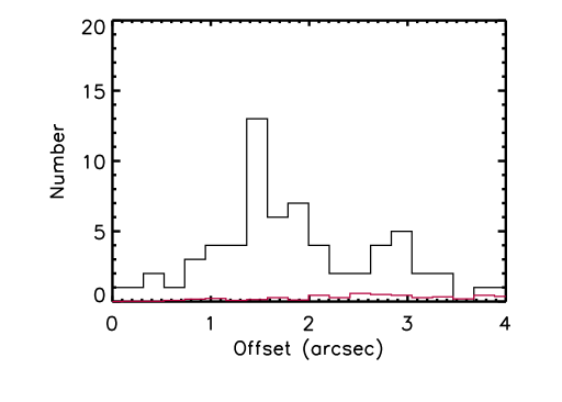
Figure 2: Offsets between the 65 SCUBA-2 450 $\mu$m centroid positions and the radio positions for counterparts within $4^{\prime\prime}$. The mean offset is $2\farcs 0$, and the median offset is $1\farcs 7$. The red curve shows the histogram of offsets that would be expected between the positions of a random distribution of 450 $\mu$m sources and the radio positions for counterparts within $4^{\prime\prime}$, based on 64 simulations.

For the GOODS-S, we use the VLA 20 cm catalog of Miller et al. (2013) of the Extended CDF-S, which covers an area of about a third of a square degree and reaches a best rms sensitivity of 6 $\mu$Jy. Their catalog contains 883 distinct radio sources. For this field, we do our absolute astrometric pointing check and offset calculation using the ALMA data (see Section 2.3).

2.3 ALMA 870 $\mu$m Observations of the GOODS-S

In the most sensitive 100 arcmin² area, all of the $>2.25$ mJy SCUBA-2 850 $\mu$m sources ($>4\sigma$) have been observed with ALMA in band 7 (870 $\mu$m), together with a number of fainter SCUBA-2 sources. Details of these observations and their reductions may be found in Cowie et al. (2018). We restrict the area of the individual ALMA images to their FWHM radius of $8\farcs 75$. With this restriction, the ALMA images cover a (non-contiguous) total area of 7.2 arcmin². We used these data in analyzing the SCUBA-2 850 $\mu$m sources in Cowie et al. (2018) and Barger et al. (2019).

Note that some of the ALMA sources are off the 450 $\mu$m area that we use in this paper (see Section 2.1). Based on the mean offset of 11 isolated ALMA sources with 870 $\mu$m fluxes $>2.25$ mJy from the nearest SCUBA-2 450 $\mu$m peak, we found an absolute astrometric offset of $1\farcs 44$ in R.A. and $1\farcs 28$ in Decl., which we applied to the SCUBA-2 450 $\mu$m positions in Table 3. This is well within the expected uncertainty in the absolute SCUBA-2 450 $\mu$m astrometry.

In Figure 3(a), we show the ALMA observed areas (gray circles) with the SCUBA-2 450 $\mu$m source positions overlaid (red squares). 13 of the 16 450 $\mu$m sources lie on an ALMA image. In Figure 3(b), we show the ALMA sources convolved with the SCUBA-2 850 $\mu$m PSF with the 450 $\mu$m source positions again overlaid (red squares). 12 of the 13 450 $\mu$m sources that lie on an ALMA image have an ALMA source counterpart within $4^{\prime\prime}$; the remaining 450 $\mu$m source lies on the edge of an ALMA image, as noted in Table 3. In Figure 3(c), we show the 450 $\mu$m image with the ALMA $>2.25$ mJy source positions overlaid (white squares). Some of the 450 $\mu$m sources do not correspond to the ALMA $>2.25$ mJy sample, and some of the ALMA $>2.25$ mJy sample do not have 450 $\mu$m counterparts at our current sensitivity level.

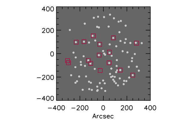
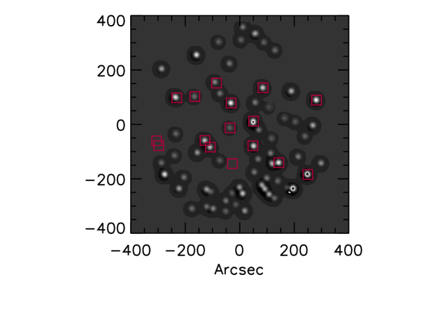
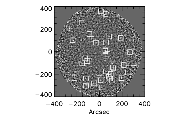
Figure 3: (a) ALMA observed areas and (b) ALMA sources convolved with SCUBA-2 850 $\mu$m PSF. The 450 $\mu$m source positions are overlaid in both panels (red squares). (c) 450 $\mu$m image with the ALMA $>2.25$ mJy source positions overlaid (white squares). The images are centered at R.A. $=3^{\rm h}32^{\rm m}26^{\rm s}$, decl. $=-27^{\circ}48^{\prime}17^{\prime\prime}$, with the x-axis (y-axis) corresponding to offsets in R.A. (decl.) from this position.

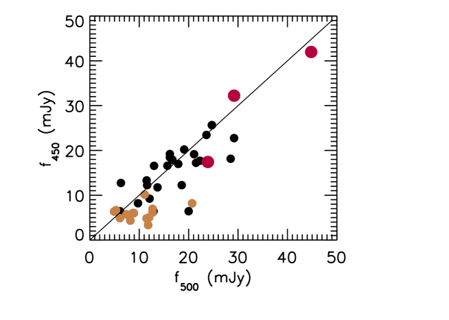
Figure 4: (a) Herschel 500 $\mu$m flux from the E11 GOODS-N catalog vs. SCUBA-2 450 $\mu$m flux from Table 2 for the 63 450 $\mu$m sources with noise $<2.8$ mJy (twice the minimum noise). Black circles denote 450 $\mu$m sources with a 500 $\mu$m counterpart within $3\farcs 5$ of the 450 $\mu$m position. Plus signs show the remaining sources at the bottom (a slight vertical offset separates sources $>12$ mJy from those $<12$ mJy). For sources 1 and 6 in Table 2, each of which has a very nearby second source, we show the combined 450 $\mu$m flux. The plotted flux uncertainties are $1\sigma$ at both 450 $\mu$m and 500 $\mu$m. (b) SCUBA-2 450 $\mu$m flux vs. Herschel 500 $\mu$m flux for all sources in the E11 catalog that lie in the SCUBA-2 area with 450 $\mu$m noise $<2.8$ mJy. Black circles show 500 $\mu$m sources with a 450 $\mu$m counterpart within $12^{\prime\prime}$ of the 500 $\mu$m source position. Red circles show 500 $\mu$m sources with multiple 450 $\mu$m counterparts within $12^{\prime\prime}$ of the 500 $\mu$m source; in these cases we use the combined 450 $\mu$m flux. Gold circles show 500 $\mu$m sources with no 450 $\mu$m counterparts in Table 2; in these cases, we measured the 450 $\mu$m fluxes directly from the image at the Herschel catalog positions.

2.4 Optical/NIR Fluxes

The GOODS fields are defined by the deep HST/ACS optical imaging of Giavalisco et al. (2004). These fields are also covered by deep CANDELS HST/WFC3 ultraviolet/optical and infrared channel imaging (Grogin et al. 2011; Koekemoer et al. 2011), and there are Spitzer/IRAC observations from the GOODS Spitzer Legacy Program (PI: M. Dickinson) and from the SEDS and S-CANDELS surveys (Ashby et al. 2013, 2015).

In the GOODS-N, we used the CANDELS/SHARDS multiwavelength catalog of Barro et al. (2019) for our photometry, after identifying counterparts to our 450 $\mu$m selected sample using a $1^{\prime\prime}$ search radius if there is an accurate position from the radio or the Submillimeter Array, and a $3^{\prime\prime}$ search radius otherwise. 55 of the 79 sources lie within the Barro et al. area and have counterparts within $1^{\prime\prime}$.

In the GOODS-S, we used the multiwavelength catalog of Guo et al. (2013) for our photometry, after identifying counterparts to our 450 $\mu$m selected sample using a $1^{\prime\prime}$ search radius if there is an accurate position from the radio or ALMA, and a $3^{\prime\prime}$ search radius otherwise. All of the sources with accurate positions lie within the Guo et al. area and have counterparts within $1^{\prime\prime}$.

2.5 MIR/FIR Fluxes

We used the catalogs of Magnelli et al. (2011) and Elbaz et al. (2011; hereafter, E11), respectively, to obtain the Spitzer/MIPS 24 $\mu$m fluxes for the GOODS-N and GOODS-S fields. These catalogs were constructed using the deep 24 $\mu$m MIPS images from the Spitzer GOODS Legacy program (PI: M. Dickinson). We used the catalogs of Magnelli et al. (2013) and E11, respectively, to obtain the Herschel/PACS 100 $\mu$m and 160 $\mu$m fluxes for the GOODS-N and GOODS-S fields. Magnelli et al. (2013) constructed the GOODS-N catalog using the combined data sets of the PACS Evolutionary Probe (PEP; Lutz et al. 2011) guaranteed time key program and the GOODS-Herschel (E11) open time key program, while E11 constructed the GOODS-S catalog using the GOODS-Herschel program data. We also used the wider area Herschel/SPIRE 250 $\mu$m, 350 $\mu$m, and 500 $\mu$m catalogs from E11 for both fields.

E11 and Magnelli et al. (2013) both used 24 $\mu$m priors to deblend the Herschel data when constructing their catalogs. They provide a detailed discussion of the robustness of the 24 $\mu$m priors in deblending the longer wavelength data. They also provide flags to assess whether sources are contaminated by nearby brighter sources.

We cross-identified the 450 $\mu$m samples with the $>20~{}\mu$Jy 24 $\mu$m sources, which are what E11 used as priors in measuring the Herschel/PACS 100 $\mu$m fluxes. For the unmatched sources, we measured the fluxes ourselves in the 24 $\mu$m images at the 450 $\mu$m positions using a $3^{\prime\prime}$ diameter aperture. We aperture corrected these 24 $\mu$m fluxes using an average correction inferred from the matched sources. We then measured fluxes in the longer wavelength data using matched-filter images, after first removing the sources in the Magnelli et al. (2011) and E11 catalogs from the images.

We examined the relative calibration of the SCUBA-2 450 $\mu$m data versus the Herschel 500 $\mu$m data using the GOODS-N data. In Figure 4(a), we plot 500 $\mu$m flux from the E11 catalog versus 450 $\mu$m flux from Table 2 for the 63 sources with noise $<2.8$ mJy. Above a 450 $\mu$m flux of 12 mJy, there are 19 sources in the figure, all but 4 of which are detected at 500 $\mu$m. Three of the non-detections at 500 $\mu$m (non-detections are shown with plus signs in the figure) have measured 350 $\mu$m fluxes, so the 500 $\mu$m fluxes are simply too faint for the catalog. The fourth (source 26 in Table 2) appears to have had its 500 $\mu$m flux allocated by E11 to a 24 $\mu$m source that is a neighbor to the correct 24 $\mu$m counterpart.

For these bright sources, the median 450 $\mu$m to 500 $\mu$m flux ratio is 1.00, and the median 450 $\mu$m to 350 $\mu$m flux ratio is 0.68. Interpolation of the Herschel data gives a median SCUBA-2 450 $\mu$m to interpolated Herschel 450 $\mu$m flux ratio of 0.90, so the SCUBA-2 data are slightly fainter on average than the Herschel data. However, the difference is well within the calibration uncertainty in both data sets. There is also uncertainty due to the Herschel deblending, which is hard to quantify.

Below a 450 $\mu$m flux of 12 mJy, there are 38 non-detections at 500 $\mu$m in the figure. This shows SCUBA-2’s ability to probe deeper than the Herschel data.

Conversely, we can measure the 450 $\mu$m counterparts to the 500 $\mu$m sources in order to understand the Herschel selection. In Figure 4(b), we plot 450 $\mu$m flux versus 500 $\mu$m flux for all sources in the E11 GOODS-N catalog that lie in the SCUBA-2 area with 450 $\mu$m noise $<2.8$ mJy. Blends of multiple 450 $\mu$m sources at the Herschel resolution are seen for some of the brightest sources (red circles). Sources with offsets from the diagonal line may have flux contributions from 450 $\mu$m counterparts that are below our flux threshold. The gold circles show sources detected in the Herschel 500 $\mu$m catalog that are not present in our SCUBA-2 450 $\mu$m catalog. For these sources, we measured the 450 $\mu$m fluxes directly from the image at the Herschel catalog positions. These 450 $\mu$m sources may be multiples, where the Herschel flux is combining sources that are below our 450 $\mu$m flux threshold, and where single-position measurements continue to underestimate the total 450 $\mu$m flux. While Herschel may be able to pick up such sources, which are not included in our catalog, it is important to stress that one is not learning about individual SMGs from such data.

2.6 Redshifts

We have been compiling spectroscopic redshifts (speczs) from our own Keck observations and from the literature for sources in the GOODS fields for many years, so we have a large database from which to draw from to find redshifts.

In the GOODS-N, many of the speczs were already presented in the SCUBA-2 850 $\mu$m and 450 $\mu$m tables of Cowie et al. (2017) (i.e., their Tables 5 and 6, respectively). The literature references from which these were drawn include Cohen et al. (2000), Cowie et al. (2004, 2016), Swinbank et al. (2004), Wirth et al. (2004, 2015), Chapman et al. (2005), Treu et al. (2005), Reddy et al. (2006), Barger et al. (2008), Pope et al. (2008), Trouille et al. (2008), Daddi et al. (2009a,b), Cooper et al. (2011), Walter et al. (2012), Bothwell et al. (2013), Momcheva et al. (2016), and Riechers et al. (2020). There are also three new NOEMA redshifts from Jones et al. (2021).

In the GOODS-S, all of the speczs were already presented in the ALMA redshift table of Cowie et al. (2018) (i.e., their Table 5), apart from one, which we obtained from later Keck/DEIMOS observations. The references for the other redshifts are Szokoly et al. (2004), Casey et al. (2012), Kurk et al. (2013), Inami et al. (2017), and Franco et al. (2018; including B. Mobasher 2018, private communication and G. Brammer 2018, private communication).

In cases where we do not have a specz, we use photometric redshift estimates (photzs) from the literature, though we caution that there is considerable scatter in the estimates from different literature catalogs for optical/NIR faint SMGs (see, e.g., Cowie et al. 2018). For the GOODS-N, we adopt the photzs from the 3D-HST survey of Momcheva et al. (2016), who used a combination of multiband photometry and G141 2D spectral data. We supplement these with photzs from Yang et al. (2014), who used the EAZY code (Brammer et al. 2008) to fit 15 broadbands from the $U$-band to the infrared (IRAC 4.5 $\mu$m) over the Hawaii-Hubble Deep Field North (Capak et al. 2004). For these, we only use the photzs that satisfy their quality flag $Q_{z}<1$.

For the GOODS-S, we adopt the photzs from Straatman et al. (2016), who used EAZY to fit the extensive ZFOURGE catalog from 0.3 to 8 $\mu$m. None of the photzs in our sample exceed their quality flag $Q<3$.

We show the redshift distribution for the 450 $\mu$m selected combined GOODS sample in Figure 5. After excluding the 16 sources without either a specz or a photz, the median redshift for the remaining 73 sources is $z=1.99$ with a 68 percent confidence range from 1.55 to 2.10. This is consistent with the median redshifts of $z=1.95\pm 0.19$ from Casey et al. (2013) and $z=1.66\pm 0.18$ from Zavala et al. (2018). However, as we will discuss in Section 4, median redshifts are not too meaningful when there is such a wide spread in the redshift distribution of the sample.

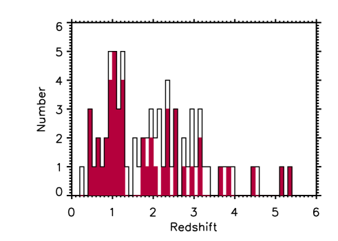
Figure 5: Histogram of the redshift distribution for the 450 $\mu$m selected combined GOODS sample. There are 16 sources without either a specz (red shaded histogram) or a photz (open histogram).

3 450 $\mu$m Number Counts

In order to test the flux calibration and consistency with previous number counts, we construct the differential number counts at 450 $\mu$m. Each source contributes $1/(A_{e}(S)dS)$ to the counts, where $A_{e}$ is the effective area where the source can be detected at $>4\sigma$ given its measured flux density $S$, and $dS$ is the flux density interval. The error is taken to be Poissonian. We show the raw differential 450 $\mu$m number counts for both fields in Figure 6(a), where we compare them with the raw STUDIES counts (Wang et al. 2017; green triangles).

There are observational biases that affect the raw counts. These include flux boosting from Eddington bias (Eddington 1913), spurious sources, source blending, and detection incompleteness. In order to correct the raw counts for these effects to obtain the intrinsic counts, we need to perform Monte Carlo simulations. We do this by first generating source-free maps with only pure noise for each of our fields. These pure noise maps are sometimes referred to as jackknife maps in the literature (see, e.g., Cowie et al. 2002). Following Chen et al. (2013a, 2013b), for each field, we subtract two maps that were each produced by coadding roughly half of the flux-calibrated data. This process subtracts off the real sources, leaving residual maps that are free of any sources. We then rescale the value of each pixel by a factor of $\sqrt{t_{1}\times t_{2}}/(t_{1}+t_{2})$, with $t_{1}$ and $t_{2}$ representing the integration time of each pixel from the two maps.

Next, we generate 40 simulated maps for each field by randomly populating our pure noise maps with the same number of sources as in our $>4\sigma$ samples. We draw these sources from the best-fit broken power law count model of Hsu et al. (2016),

$${dN\over dS}=\begin{dcases}N_{0}\Bigl{(}{S\over S_{0}}\Bigr{)}^{-\alpha}\quad\text{if}\quad S\leq S_{0}\\ N_{0}\Bigl{(}{S\over S_{0}}\Bigr{)}^{-\beta}\quad\text{if}\quad S>S_{0}\\ \end{dcases}$$ (1)

where $N_{0}=33.3$, $S_{0}=20.1$, $\alpha=2.34$, and $\beta=5.06$.

For each simulated map, we rerun our source extraction down to the $4\sigma$ threshold and compute the recovered counts using the same method and flux bins used for the science map. We compare the ratio of the total number of sources from the simulated maps with the input counts. We use all 40 simulations to determine the average ratios as a function of flux, which we then apply to the raw counts to get the corrected counts. We show the corrected number counts for both fields in Figure 6(b), where we compare them with the corrected STUDIES counts (Wang et al. 2017; green triangles).

By using SCUBA-2 observations of cluster fields (A1689, A2390, A370, MACSJ0717.5+3745, MACSJ1149.5+2223, and MACSJ1423.8+2404), Hsu et al. (2016) were able to construct the 450 $\mu$m number counts for flux detections ($>3\sigma$) down to fainter than 1 mJy, thanks to gravitational lensing effects. They used three blank fields (CDF-N, CDF-S, and COSMOS) to cover the brighter fluxes. We show their corrected number counts (black solid circles) and best-fit broken power law (black lines) in both panels of Figure 6. The consistency with Hsu et al. (2016) means it is not necessary to iterate on the input counts. A multiplicative error of 1.15 in the flux normalization in either direction would result in a significant discrepancy relative to previous counts. We note that the 450 $\mu$m counts are very uniform across fields, which is also seen by W.-H. Wang (private communication).

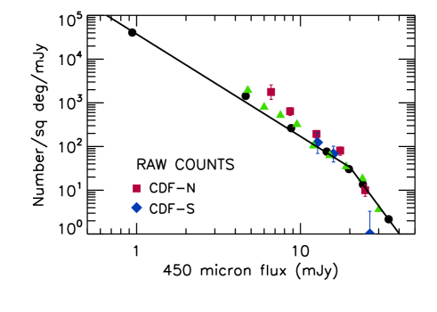
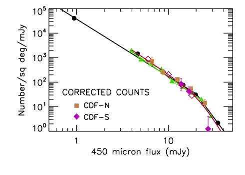
Figure 6: Differential 450 $\mu$m (a) raw number counts (red solid squares—CDF-N; blue solid diamonds—CDF-S; green solid triangles—STUDIES from Wang et al. 2017) and (b) corrected number counts (orange solid squares—CDF-N; purple solid diamonds—CDF-S; green solid triangles—STUDIES from Wang et al.; open diamonds—S2CLS EGS from Zavala et al. 2017). In both panels, the Hsu et al. (2016) corrected number counts (black solid circles) and best-fit broken power law (black lines) are shown.

4 Flux Ratios

The empirical observation of a tight correlation between thermal dust emission and radio continuum emission (e.g., Helou et al. 1985; Condon et al. 1991), known as the FIR-radio correlation, is thought to result from both quantities being linearly related to the massive SFR (Condon 1992), although we have no good theoretical understanding of the correlation. If this correlation continues to hold at high redshifts, as evidence suggests it does at least out to $z\sim 5$ (e.g., Barger et al. 2012, 2015; Thomson et al. 2014; Lim et al. 2020), then very sensitive radio observations can be used to localize distant galaxies detected in the submillimeter. In the early days of trying to understand the SCUBA sources, 20 cm data from the VLA were used for just this purpose (e.g., Barger et al. 2000; Smail et al. 2000; Chapman et al. 2003). In combination with the submillimeter data, the 20 cm data have the advantage of allowing crude redshift estimates (sometimes called millimetric redshifts) to be made, based on the opposing spectral slopes of the blackbody spectrum in the submillimeter and the synchrotron spectrum in the radio (e.g., Carilli & Yun 1999; Barger et al. 2000).

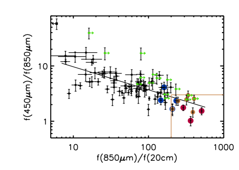
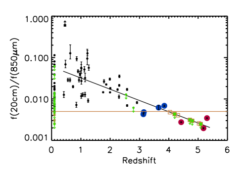
Figure 7: Based on our 450 $\mu$m selected combined GOODS sample: (a) 450 $\mu$m to 850 $\mu$m flux ratio (uncertainties from the 450 $\mu$m measurements) vs. 850 $\mu$m to 20 cm flux ratio (uncertainties from the 850 $\mu$m measurements) for sources with radio data, (b) 20 cm to 850 $\mu$m flux ratio vs. redshift (uncertainties from the 850 $\mu$m measurements) for sources with radio data, and (c) 450 $\mu$m to 850 $\mu$m flux ratio vs. redshift (uncertainties from the 450 $\mu$m measurements). Sources with only radio limits are shown in green with (a) rightward-pointing arrows and (b) downward-pointing arrows. In (b) and (c), sources without speczs are placed at a nominal redshift of $z=0.1$ and shown without uncertainties, for clarity. In all panels, solid lines show simple linear fits to the data, without considering uncertainties and after excluding GOODS-N source 70, which is at the top-left of each plot (black square; arrows denote when its value is off the plot). Sources with $3\leq z_{spec}<4$ are shown in blue, while those with $z_{spec}\geq 4$ are shown in red. Our adopted high-redshift selection criteria are denoted by gold lines, and the sources that satisfy the (a) combined or (b) and (c) individual criteria but do not have speczs are colored gold. In (b) and (c), we estimate where these sources would lie in redshift based on the given linear fit (gold open squares).

FIR/submillimeter flux ratios have also been used to estimate redshifts. For example, Figure 19 of Cowie et al. (2017) showed that for their 850 $\mu$m sample in the GOODS-N, $f_{20~{}{\rm cm}}/f_{850~{}\mu{\rm m}}$ and $f_{250~{}\mu{\rm m}}/f_{850~{}\mu{\rm m}}$ were well correlated, suggesting that both provide a measure of the redshifts. They also found that those with speczs were well segregated by redshift interval. Interestingly, they determined that the scatter in specz versus $f_{20~{}{\rm cm}}/f_{850~{}\mu{\rm m}}$ was considerably larger than the scatter in specz versus $f_{250~{}\mu{\rm m}}/f_{850~{}\mu{\rm m}}$ (their Figure 20). This is a clear indication that the radio power is not always an accurate measure of the star formation (see Barger et al. 2017 for a detailed analysis of the star-forming galaxies and AGNs in the GOODS-N that lie on the FIR-radio correlation). In contrast, the scatter in specz versus $f_{250~{}\mu{\rm m}}/f_{850~{}\mu{\rm m}}$ is primarily caused by variations in the SEDs of the sources.

Other authors (e.g., Casey et al. 2013; Wang et al. 2019; Lim et al. 2020) have constructed the flux ratios for SMGs in COSMOS and compared them with optical/NIR photzs. Of particular interest is the identification of high-redshift sources. For example, Wang et al. plotted $f_{870~{}\mu{\rm m}}/f_{450~{}\mu{\rm m}}$ versus $z_{phot}\gtrsim 3$ for their ALMA-detected $H$-dropouts in their Extended Data Figure 4.

To look for high-redshift candidates in our 450 $\mu$m selected combined GOODS sample, in Figure 7(a), we plot $f_{450~{}\mu{\rm m}}/f_{850~{}\mu{\rm m}}$ versus $f_{850~{}\mu{\rm m}}/f_{20~{}{\rm cm}}$. We color-code the $3\leq z_{spec}<4$ (blue large circles) and $z_{spec}\geq 4$ sources (red large circles). We adopt the uncertainties on the 450 $\mu$m fluxes in the y-axis, since we expect them to be larger than the uncertainties on the 850 $\mu$m fluxes, and we adopt the uncertainties on the 850 $\mu$m fluxes in the x-axis, since we expect them to be larger than the uncertainties on the 20 cm fluxes. We assign the 20 cm ($>5\sigma$) flux limits of the two samples to the sources in the radio areas without radio detections (green rightward-pointing arrows).

We can see the good relation between the two flux ratios. A linear fit without considering uncertainties and after excluding source 70, which is located at the top-left of the plot, gives $\log($$f_{450~{}\mu{\rm m}}/f_{850~{}\mu{\rm m}}$)$=-0.42\log($$f_{850~{}\mu{\rm m}}/f_{20~{}{\rm cm}}$$)+1.40$ (solid line).

We can also see the generally good segregation of the high-redshift sources with speczs from the rest of the population. Thus, we define high-redshift selection criteria based on this plot, namely, $f_{450~{}\mu{\rm m}}/f_{850~{}\mu{\rm m}}$$<3$ and $f_{850~{}\mu{\rm m}}/f_{20~{}{\rm cm}}$$>200$ (gold lines). Based on these criteria, we have six candidate high-redshift sources (gold large circles).

In Figures 7(b) and (c), respectively, we show the two axes from (a) separately versus redshift. We again color-code in blue and red the high-redshift sources with speczs. We plot the sources without speczs at a nominal redshift of $z=0.1$ and without uncertainties, for clarity. In (b), we again show the sources in the radio areas without radio detections as limits (green downward-pointing arrows). In both panels, we show the linear fits as solid lines without considering uncertainties and after excluding source 70, but we only include in the fits those sources having speczs. The resulting fits are (b) $\log($$f_{20~{}{\rm cm}}/f_{850~{}\mu{\rm m}}$)$=-0.27z-1.22$ and (c) $\log($$f_{450~{}\mu{\rm m}}/f_{850~{}\mu{\rm m}}$)$=-0.16z+0.96$.

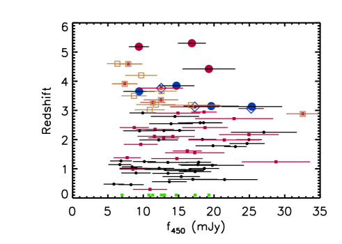
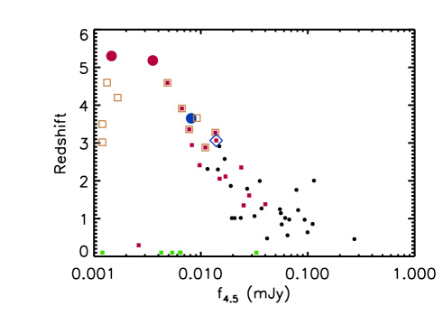
Figure 8: (a) Redshift vs. 450 $\mu$m flux (with uncertainties) for the 450 $\mu$m selected combined GOODS sample. (b) Redshift vs. 4.5 $\mu$m flux for the sources in the 450 $\mu$m selected GOODS-N sample that lie within the HST/ACS footprint. We use the Barro et al. (2019) catalog for most of the 4.5 $\mu$m fluxes, but for the small number of sources not in that catalog, we measured the fluxes ourselves. Note that the uncertainties on the 4.5 $\mu$m fluxes are smaller than the data points. In both panels, sources with speczs $<3$ are shown as black circles, while sources with photzs are shown as red squares. Sources with $3\leq z_{spec}<4$ are denoted by blue large circles, while those with $z_{spec}\geq 4$ are denoted by red large circles. The high-redshift candidates from Table 4 are denoted by gold open squares (we use the photzs for the five that have a photz). Sources with $3\leq z_{phot}<4$ that were not also identified as high-redshift candidates from the FIR are enclosed in blue large open diamonds. Finally, sources without either a specz or a photz and not identified as high-redshift candidates from the FIR are placed at a nominal redshift of $z=0.1$ and shown as green squares without uncertainties, for clarity.

In each figure, we show the relevant high-redshift criterion from Figure 7(a) as a gold line, and we color in gold the sources that satisfy it. In (b), we have the same high-redshift candidates as in (a), plus one additional candidate. Note that we conservatively consider only a radio limit that is already below the gold line to be a candidate high-redshift source. In (c), we have the same high-redshift candidates as in (a), plus five additional candidates, none of which is the additional candidate found in (b). In both (b) and (c), we plot gold open squares at the redshifts we estimate from the linear fits.

c

Figure 9: All 450 $\mu$m selected sources in the GOODS-S (i.e., Table 3; source numbers on bottom) that lie in the CANDELS region. (Right in each panel): Multiwavelength SEDs (green—HST and Spitzer/IRAC optical/NIR; pink—Spitzer/MIPS 24 $\mu$m; blue—Herschel FIR; red—SCUBA-2 450 $\mu$m; gold—ALMA 870 $\mu$m; black—ALMA 1.1 mm) and MAGPHYS fit (black curve). The SED plots are labeled at the top-right with the source number and at the top-left with the specz or the photz, the $\chi^{2}$ value for the fit, and the SFR. (Left in each panel): two thumbnail images showing (top) a combination of Herschel/PACS 100 $\mu$m (blue), SCUBA-2 450 $\mu$m (green), and SCUBA-2 850 $\mu$m (red) data, and (bottom) a combination of HST F435W (blue), F814W (green), and F160W (red) data. The contours are ALMA 870 $\mu$m. Note that the ALMA position for source 4 is on the edge of another source (see bottom-left thumbnail), so no SED was constructed due to contamination of the photometry.

In Table 4, we list the 12 high-redshift candidates that satisfy either the 20 cm/850 $\mu$m selection or the 450 $\mu$m/850 $\mu$m selection that we defined in Figure 7. All of these candidates come from the GOODS-N. We also give their 450 $\mu$m, 850 $\mu$m, and 20 cm fluxes; their 20 cm/850 $\mu$m and 450 $\mu$m/850 $\mu$m flux ratios; their photzs from Table 2, where available; and the redshifts we estimate from the linear fits in Figures 7(b) and (c), respectively, if the source is a high-redshift candidate based on the figure in question.

Most of the candidates are very faint in the optical/NIR and do not have reliable photzs, but for the five that have photzs, the photzs are consistent with the sources being at high redshift. In combination with three sources with $z_{phot}\geq 3$ that were not identified as high-redshift candidates in the FIR and seven sources with known $z_{spec}\geq 3$, we have a total of 22 possible high-redshift sources (we list all of these sources in Table 4).

In Figure 8(a), we show redshift versus 450 $\mu$m flux for our 450 $\mu$m selected combined GOODS sample, with the high-redshift spectroscopic sources denoted by blue and red circles, the high-redshift candidates selected from Figure 7 denoted by gold squares (5 of these also have photzs, so in those cases we use the photzs; we use $z_{450/850}$ for 6 sources; and for the last source, which was not identified as a high-redshift candidate from the 450 $\mu$m/850 $\mu$m flux ratio, we use $z_{20/850}$), and the three additional high-redshift photz sources denoted by blue diamonds. The redshift distribution at every flux is very large, demonstrating why quoting a median redshift for the sample as a whole is not particularly meaningful.

High-redshift sources can also be picked out by their faintness in the MIR. In Figure 8(b), we plot redshift versus 4.5 $\mu$m flux for the 450 $\mu$m selected sample lying within the HST/ACS footprint of the GOODS-N. We used the Barro et al. (2019) catalog for the 4.5 $\mu$m fluxes. For the small number of sources not in the catalog, we measured the 4.5 $\mu$m fluxes on the Spitzer/IRAC image using a $3^{\prime\prime}$ diameter aperture and obtained the normalization by matching to sources in the catalog.

For the sources with a measured 4.5 $\mu$m flux and either a specz, a photz, or a FIR redshift from Table 4, there is a strong correlation of redshift with 4.5 $\mu$m flux, with all of the $z\geq 3$ sources having fluxes below 0.014 mJy. This alternate high-redshift diagnostic provides a strong confirmation of the high-redshift candidate selection from the FIR.

It is clear that using FIR methods to identify high-redshift candidates that cannot be found with photzs is critical, or else the redshift distribution for 450 $\mu$m selected samples will not be complete and will be biased to lower redshifts.

5 SED Fitting

We next want to determine the SFRs and dust temperatures of the 450 $\mu$m selected samples. We obtain best fits to the SMGs’ full SEDs using the publicly available Bayesian energy-balance SED-fitting code MAGPHYS (da Cunha et al. 2015). We fit at the adopted redshifts (see Section 2.6), and we do not allow the redshift to vary to optimize the SED fit. The SED fits give SFRs (from the total bolometric luminosities; these are 100 Myr averages for a Chabrier 2003 initial mass function, or IMF) and dust properties, together with their error ranges. We note that SFRs are relatively insensitive to redshift for dust-dominated galaxies.

For illustrative purposes, in Figure 9, we show the SEDs (colored symbols) and the MAGPHYS fits (black curve) for each 450 $\mu$m source in the GOODS-S sample (i.e., Table 3) that lies in the CANDELS region, alongside two multiwavelength thumbnails (FIR/submillimeter on top and optical/NIR on bottom). The SED plots are labeled at the top with the specz or photz, the $\chi^{2}$ value for the fit, and the SFR. Note that there is no SED plot for source 4, since the ALMA position for that source is on the edge of another source, and thus the photometry is contaminated.

The MAGPHYS infrared SEDs contain multiple temperature components, which provide an average, luminosity-weighted dust temperature (see da Cunha et al. 2015’s Equation 8). We shall generally adopt these temperatures. However, we note that at low redshifts, where the short wavelength FIR data are relatively unconstraining, MAGPHYS may insert hot components that raise the temperatures and FIR luminosities. In order to check the reality of these components, we also constructed gray body fits for our 450 $\mu$m selected GOODS-N sample using an optically thin, single temperature modified blackbody, $S_{\nu}\propto\nu^{\beta}B_{\nu}(T)$ (e.g., see Klaas et al. 1997). Both the MAGPHYS and the gray body fits assume $\beta=1.5$.

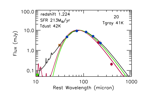
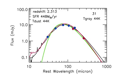
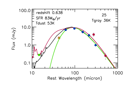
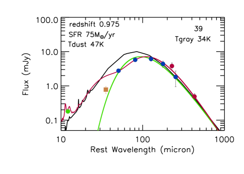
Figure 10: SEDs for four example sources from the 450 $\mu$m selected GOODS-N sample. Where available, we show the 70 $\mu$m flux with gold squares. The curves are Arp 220 (black), MAGPHYS fits (red), and gray body fits (green). (Top row) Two higher-redshift examples where the MAGPHYS and gray body fits are consistent and also similar to Arp 220. (Bottom row) Two lower-redshift examples where the MAGPHYS fit includes a hot component that is inconsistent with the 70 $\mu$m flux.

Fourteen of the sources have observed-frame 70 $\mu$m fluxes, and these fluxes were not used in either the MAGPHYS or the gray body fits. In Figure 10, we show example comparisons of the two fits (MAGPHYS in red and gray body in green), along with an Arp 220 SED (black). For the two higher-redshift sources shown (top row; sources 20 and 31), the MAGPHYS and gray body fits are similar and return nearly identical dust temperatures. Source 20 has a 70 $\mu$m measurement (gold square) consistent with the fitted SED; source 31 does not have a 70 $\mu$m measurement. However, for the two lower-redshift sources (bottom row; sources 25 and 39), MAGPHYS includes a hot component that substantially raises the temperature above the gray body fit. Both of these sources have 70 $\mu$m measurements that are strongly inconsistent with the MAGPHYS SED but agree roughly with the gray body fits.

We conclude that the gray body fits are preferred at lower redshifts, noting that this also reduces the FIR luminosities and SFRs for these sources. In our subsequent analyses, we will adopt the SFRs and dust temperatures derived from the gray body fits when we extend to sources below $z=1$.

6 MAGPHYS Star Formation Rates and FIR Luminosities

In this section, we examine the SFRs and FIR luminosities that MAGPHYS outputs for the 450 $\mu$m selected combined GOODS sample sources with $z>1$.

In Figure 11(a), we plot $L_{8-1000~{}\mu{\rm m}}$ versus SFR. A simple linear fit gives

$$\log{\rm SFR}(M_{\odot}~{}{\rm yr^{-1}})=\log L_{8-1000~{}\mu{\rm m}}{\rm(erg~{}s^{-1})}-43.71\,,$$ (2)

which we denote on the figure by a solid line. For comparison, Murphy et al. (2011) determined a theoretical conversion of $-43.41$ between the two terms, which they computed from a Starburst99 (Leitherer et al. 1999) constant SFR model and a Kroupa (2001) IMF. For a Chabrier IMF, this would correspond to $-43.38$. We denote this relation by the dashed line. Meanwhile, Madau & Dickinson (2014) adopted $-43.52$ using Kennicutt (1998), after conversion to a Chabrier IMF from their Salpeter (1955) IMF. We denote this relation by the dotted line. Both of these relations give slightly lower SFRs than the MAGPHYS relation. This emphasizes the uncertainty in the $L_{8-1000~{}\mu{\rm m}}$ to SFR calibration.

In Figure 11(b), we verify empirical expectations for a correlation between $L_{8-1000~{}\mu{\rm m}}$ and radio power. We determine the latter independently of MAGPHYS using

$$P_{\rm 20~{}cm}=4\pi{d_{L}}^{2}f_{\rm 20\,cm}10^{-29}(1+z)^{\alpha-1}~{}{\rm erg~{}s}^{-1}~{}Hz^{-1}\,.$$ (3)

Here $d_{L}$ is the luminosity distance (cm) and $f_{20\,{\rm cm}}$ is the 20 cm flux in units of $\mu$Jy. This equation assumes that the radio flux density goes as $\nu^{-\alpha}$. Following Barger et al. (2017), we adopt a radio spectral index of $\alpha=0.8$ (Condon 1992; Ibar et al. 2010; An et al. 2021). The solid line shows the median FIR-radio correlation for star-forming galaxies from Barger et al., and the dotted lines show a multiplicative factor of 3 of this value, which Barger et al. considered to be the region where sources lie on the FIR-radio correlation. The current data are well-represented by the Barger et al. correlation.

In Figure 11(c), we plot SFR versus SCUBA-2 850 $\mu$m flux. A simple linear fit to the data, not considering uncertainties on the data, gives

$$\log{\rm SFR}=1.12\log f_{850~{}\mu{\rm m}}+1.70\,,$$ (4)

which we denote on the figure by a solid line. There may be a shift to higher SFRs for brighter sources in our sample. The slope in our relation is steeper than that in Dudzevic̆iūtė et al. (2020), who found

$$\log{\rm SFR}=0.42\log f_{870~{}\mu{\rm m}}+2.19$$ (5)

for 517 AS2UDS sources with redshifts between $z=1.8$ and $z=3.4$. We denote their relation on the figure as a dashed line. The reason for the disagreement is not clear.

In Figure 11(d), we plot SFR versus redshift. The present results are broadly consistent with the maximum SFR from Barger et al. (2017), namely 1000 M_⊙ yr^-1 (dashed line), above which there are relatively few galaxies (see also Karim et al. 2013 and Barger et al. 2014). The Barger et al. (2017) value is based on the Murphy et al. (2011) relation and a Kroupa IMF, and the primary uncertainty is the calibration of the SFR.

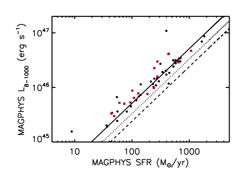
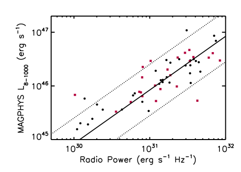
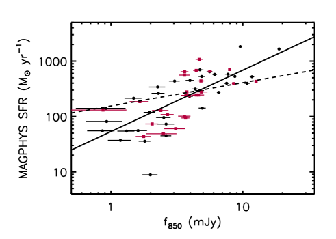
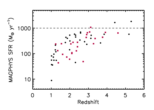
Figure 11: Based on the 450 $\mu$m selected combined GOODS sample with either $z_{spec}>1$ or a $z_{phot}>1$: (a) MAGPHYS FIR luminosity vs. MAGPHYS SFR, (b) MAGPHYS FIR luminosity vs. radio power, (c) MAGPHYS SFR vs. SCUBA-2 850 $\mu$m flux (with uncertainties on the flux), and (d) MAGPHYS SFR vs. redshift. Sources with speczs are shown as black circles, while sources with photzs are shown as red squares. In (a), the solid line shows a simple linear fit to the two MAGPHYS outputs, while the dashed line shows the relation (after conversion to a Chabrier IMF) from Murphy et al. (2011; their Equation 4), and the dotted line shows the relation (after conversion to a Chabrier IMF) adopted by Madau & Dickinson (2014), which is based on Kennicutt (1998). In (b), the solid line shows the median FIR-radio correlation for star-forming galaxies from Barger et al. (2017) (calculated from their Equation 3, using a parameterization of 2.35, and their Equation 4), and the dotted lines show a multiplicative factor of 3 of this value, which they considered to be the region where sources lie on the FIR-radio correlation. In (c), the solid line shows shows a simple linear fit to the data (this paper’s Equation 4), and the dashed line shows, for comparison, the linear relation from Dudzevic̆iūtė et al. (2020) (given in this paper’s Equation 5). In (d), the dashed line shows the maximum SFR for galaxies from Barger et al. (2017) based on the Murphy et al. (2011) relation and a Kroupa IMF, which is very similar to a Chabrier IMF (see text in Section 6).

7 Discussion

Most comparisons of 450 $\mu$m and 850 $\mu$m selected samples have argued that the 450 $\mu$m samples peak at lower redshifts (e.g., Casey et al. 2013; Zavala et al. 2018; Lim et al. 2020) and may be biased to higher dust temperatures (Casey et al. 2013; Lim et al. 2020). Such sample differences are clearly introduced by the SED shape, where $f_{450~{}\mu{\rm m}}/f_{850~{}\mu{\rm m}}$ becomes smaller as one moves to higher redshifts (see Figure 7(c)) and larger as one moves to higher dust temperatures. However, as Lim et al. (2020) emphasize, these selection biases are very dependent on the relative depths of the 450 $\mu$m and 850 $\mu$m samples, since the dust temperature is strongly dependent on the FIR luminosity, and submillimeter samples are biased to higher FIR luminosities at higher redshifts.

7.1 Are the Redshift Distributions Different for a 450 $\mu$m versus an 850 $\mu$m Selection?

In Figure12(a), we show the 850 $\mu$m fluxes from Tables 2 and 3 measured for the 450 $\mu$m selected combined GOODS sample versus redshift. The horizontal line shows the SCUBA-2 1.65 mJy ($4\sigma$) confusion limit at 850 $\mu$m. As was also noted by Zavala et al. (2018), all of the sources above $z=1.5$ (vertical line) would be included in an 850 $\mu$m sample, and the 450 $\mu$m selection only adds sources that would not be found in an 850 $\mu$m sample below $z=1.5$.

In Figure 12(b) (bottom histogram), we show the redshift distribution of the 450 $\mu$m selected combined GOODS sample (black line histogram). The red shading shows the sources in this sample that are detected above 1.65 mJy at 850 $\mu$m. In Figure 12(b) (top histogram), we show the redshift distribution of the 58 sources with fluxes $>1.65$ mJy in the GOODS-S ALMA 870 $\mu$m sample of Cowie et al. (2018) (blue histogram). A Mann-Whitney test shows no statistically significant difference between the blue histogram and the red histogram.

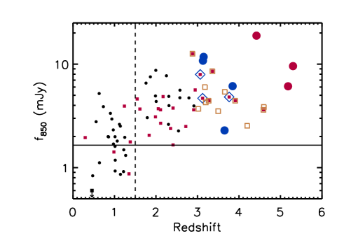
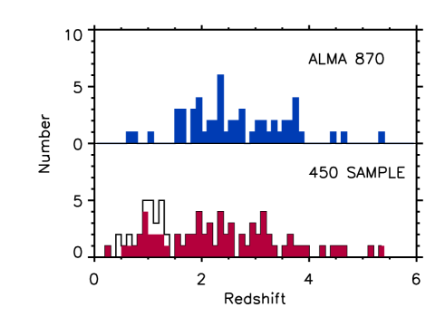
Figure 12: (a) SCUBA-2 850 $\mu$m flux vs. redshift for the 450 $\mu$m selected combined GOODS sample. Sources with $z_{spec}<3$ are shown as black circles, while sources with $z_{phot}$ are shown as red squares. Sources with $3\leq z_{spec}<4$ are denoted by blue large circles, while those with $z_{spec}\geq 4$ are denoted by red large circles. The high-redshift candidates from Table 4 are denoted by gold open squares (we use the photzs for the five that have a photz). Sources with $3\leq z_{phot}<4$ that were not also identified as high-redshift candidates from the FIR are enclosed in blue large open diamonds. GOODS-N source 70 (bottom-left of the plot) is denoted by a black square with a downward pointing arrow, indicating it is off the plot. The horizontal line shows the SCUBA-2 1.65 mJy ($4\sigma$) confusion limit at 850 $\mu$m, and the dashed vertical line shows the redshift $z=1.5$ above which all of the 450 $\mu$m sources would be found in an 850 $\mu$m sample. (b) Redshift distributions for the 450 $\mu$m selected combined GOODS sample (bottom histogram; shaded region shows the sample that has SCUBA-2 850 $\mu$m fluxes $>1.65$ mJy) and for the $>1.65$ mJy ALMA 870 $\mu$m GOODS-S sample of Cowie et al. (2018) (top histogram). We do not show the eight 450 $\mu$m sources without any redshift information in either (a) or (b).

Restricting the 450 $\mu$m selected sample to sources that would be present in the SCUBA-2 confusion-limited ($>1.65$ mJy) 850 $\mu$m selected sample raises the median redshift to $z=2.30$ from the $z=1.99$ value noted previously for the full 450 $\mu$m sample. However, as we have emphasized, there is a wide distribution of redshifts, and the median is a poor characterization of this distribution.

This situation is best summarized by noting that the two distributions are quite similar for the higher redshift sources, but the 450 $\mu$m sample adds in lower redshift sources, which results in the reduction of the median.

7.2 Do Dust Temperatures Evolve with Redshift?

Many previous papers have noted strong evolution in dust temperature with both redshift and FIR luminosity (e.g., Magnelli et al. 2013; Swinbank et al. 2014; Béthermin et al. 2015; Schreiber et al. 2018; Zavala et al. 2018). If the effective area over which the galaxy radiated were constant as a function of both redshift and FIR luminosity, then there would be a simple monotonic relation between FIR luminosity and dust temperature. However, when we measure the evolution of FIR luminosity, we are also measuring the evolution in the galaxy properties. There is a dependence of FIR luminosity on dust temperature, but it is not the sole dependence.

We show the evolution in dust temperature for the present 450 $\mu$m selected GOODS-N sample in Figures 13(a) and 13(b), respectively. In both panels, we code the data points by redshift. From Figure 13(a), we see that there is a strong increase in dust temperature with redshift. From Figure 13(b), we see that there is a strong increase in dust temperature with FIR luminosity.

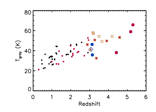
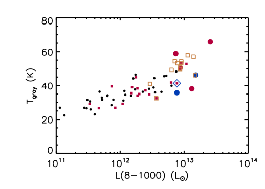
Figure 13: Gray body dust temperature vs. (a) redshift and (b) $L_{8-1000~{}\mu{\rm m}}$ for our 450 $\mu$m selected GOODS-N sample with gray body temperature measurements. Sources with $z_{spec}<3$ are shown as black small circles. Sources with $z_{phot}$ are shown as red small squares. Sources with $3\leq z_{spec}<4$ are denoted by blue large circles, while those with $z_{spec}\geq 4$ are denoted by red large circles. The high-redshift candidates from Table 4 are denoted by gold open squares (we use the photzs for the five that have a photz). A source with $3\leq z_{phot}<4$ that was not also identified as a high-redshift candidate from the FIR is enclosed in a blue large open diamond.

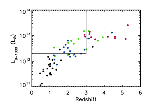
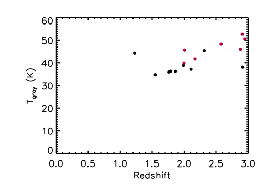
Figure 14: (a) $L_{8-1000~{}\mu{\rm m}}$ and (b) gray body dust temperature (from selected region in (a)) vs. redshift for our 450 $\mu$m selected GOODS-N sample with gray body temperature measurements. In (a), the symbols are color-coded by temperature (black$<35$ K; blue=35–40 K; green=40–50 K; red$>50$ K). The temperatures are strongly correlated with $L_{8-1000~{}\mu{\rm m}}$. The black lines show a restricted region with redshifts $z<3$ and $L_{8-1000~{}\mu{\rm m}}$ $>2\times 10^{12}~{}L_{\odot}$ where our sample should be substantially complete. In (b), we show sources from only that restricted region. The symbols are color-coded by $L_{8-1000~{}\mu{\rm m}}$ (black$>2\times 10^{12}~{}L_{\odot}$; red$>5\times 10^{12}~{}L_{\odot}$).

However, there is controversy over whether the evolution of the dust temperature with redshift is a real effect or simply a consequence of the selection bias to higher FIR luminosity as we move to higher redshifts. Most recently, Lim et al. (2020) and Dudzevic̆iūtė et al. (2020) did not find any evidence for redshift evolution in a uniform FIR luminosity subsample of their data. Using a spectroscopically complete 1.4 mm selected South Pole Telescope high-redshift, strongly gravitationally lensed sample, Reuter et al. (2020) also found that their data could be consistent with no evolution.

Our data agree with these recent results. From Figure 13(b), we can see at once that at the high FIR luminosity end for this relatively small sample, the range of dust temperatures is similar for both high ($z>3$) and more moderate ($z<3$) redshift sources. We look at this in more detail in Figure 14. Here we restrict to sources with redshifts $z<3$ and $L_{8-1000~{}\mu{\rm m}}$ $>2\times 10^{12}~{}L_{\odot}$, where we expect our sample to be substantially complete. We find no statistically significant evidence of evolution with redshift with a Pearson coefficient of $R=0.3433$.

7.3 Do 450 $\mu$m Samples Select Warmer Sources Than an 850 $\mu$m Sample?

As we discussed in Section 7.1, the 450 $\mu$m selection only adds sources that would not be found in an 850 $\mu$m sample below $z=1.5$. We characterize the evolution in $f_{450~{}\mu{\rm m}}/f_{850~{}\mu{\rm m}}$ with redshift by using the fitted MAGPHYS SEDs for the 450 $\mu$m selected GOODS-N sample sources and determining what the $f_{450~{}\mu{\rm m}}/f_{850~{}\mu{\rm m}}$ values would be if the lower-redshift sources were moved up in redshift. In Figure 15, we show predicted $f_{450~{}\mu{\rm m}}/f_{850~{}\mu{\rm m}}$ versus redshift (black curves) for all of the sources with $z<1.5$. We compare these with the measured values for all the sources with $z>1.5$ (squares; color-coded by the MAGPHYS dust temperature: blue $<40$ K; green=40–50 K; red$>50$ K). The higher-redshift sources are consistent with having the same SEDs as the lower-redshift sources (i.e., the squares lie in the range of the extrapolated lower-redshift values). Thus, there is no evidence for the selection of warmer sources with a 450 $\mu$m sample than with an 850 $\mu$m sample.

8 Summary

In this fifth paper in our SUPER GOODS series, we presented SCUBA-2 450 $\mu$m selected samples in the two GOODS fields. Our main results are as follows:

$\bullet$ We constructed the differential number counts at 450 $\mu$m and found excellent agreement with results in the literature.

$\bullet$ We used the extensive redshift information available on the GOODS fields to see how well redshifts could be estimated from simple flux ratios (20 cm/850 $\mu$m and 450 $\mu$m/850 $\mu$m). We found tight correlations for both ratios with redshift.

$\bullet$ We provided a table of 12 high-redshift candidates based on these correlations. Most of the candidates are very faint in the optical/NIR and do not have reliable photzs, but for the five that have photzs, the photzs are consistent with the sources being at high redshift.

$\bullet$ We found a strong correlation of redshift with 4.5 $\mu$m flux. This alternate high-redshift diagnostic strongly confirms our high-redshift candidate selection. Without FIR methods to identify high-redshift candidates that cannot be found with photzs, the redshift distribution for 450 $\mu$m selected samples is not complete and is biased to lower redshifts.

$\bullet$ We found a wide distribution of redshifts for the 450 $\mu$m selected sample, making the median redshift a poor characterization of this distribution.

$\bullet$ We constructed full SEDs and used the publicly available SED-fitting code MAGPHYS (da Cunha et al. 2015) to obtain best fits at our adopted redshifts. These SED fits gave SFRs and dust properties for our 450 $\mu$m selected samples.

$\bullet$ At low redshifts, MAGPHYS may insert hot components that raise the temperatures and FIR luminosities of the sources. We checked these components by also constructing gray body fits for our 450 $\mu$m selected GOODS-N sample. Through comparisons with observed-frame 70 $\mu$m fluxes that were not included in either type of fit, we concluded that the gray body fits are preferred at $z<1$.

$\bullet$ We found that the 450 $\mu$m selected sample introduces a number of $z<1.5$ sources, but beyond this, there is no difference in the redshift distributions for 450 $\mu$m and 850 $\mu$m samples.

$\bullet$ We found that the observed evolution of dust temperature with redshift is primarily driven by a selection bias of higher FIR luminosities at higher redshifts.

$\bullet$ We did not find evidence that warmer sources are selected in a 450 $\mu$m sample than in an 850 $\mu$m sample.

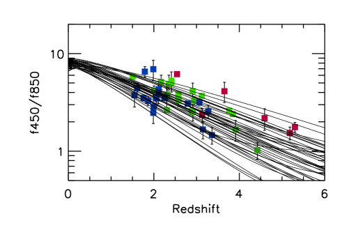
Figure 15: Predicted $f_{450~{}\mu{\rm m}}/f_{850~{}\mu{\rm m}}$ vs. redshift (black curves) for all of the 450 $\mu$m selected sources in the GOODS-N with $z<1.5$ based on the fitted MAGPHYS SEDs. Squares show the measured values for all the sources with $z>1.5$, color-coded by the MAGPHYS dust temperature (blue $<40$ K; green=40–50 K; red$>50$ K).

Table 2: CDF-N SCUBA-2 450 $\mu$m Sample ($>4\sigma$)

No. and Name	R.A.450	Decl.	450 $\mu$m	SNR	R.A.VLA	Decl.	20 cm	850 $\mu$m	$z$	offset
	(J2000.0)		(mJy)		(J2000.0)		($\mu$Jy)	(mJy)		(′′)
(1)	(2)	(3)	(4)	(5)	(6)	(7)	(8)	(9)	(10)	(11)
1 SMM 123730+621300	12 37 30.62	62 13 0.09	32.3(2.20)	14.64	12 37 30.80	62 12 58.7	123(6.1)	12.60(0.26)	2.88	1.82
2 SMM 123537+622239	12 35 37.82	62 22 39.2	28.6(4.38)	6.52	12 35 38.15	62 22 41.0	154(8.6)	3.93(0.53)	1.23	3.01
3 SMM 123546+622012	12 35 46.80	62 20 12.5	25.5(3.91)	6.53	12 35 46.66	62 20 13.4	46(6.8)	10.79(0.50)	3.132	1.32
4 SMM 123707+621408	12 37 7.309	62 14 8.29	24.4(1.69)	14.36	12 37 7.210	62 14 8.19	59(8.7)	7.95(0.20)	3.06	1.46
5 SMM 123721+620709	12 37 21.09	62 07 9.20	25.1(4.02)	6.24	12 37 21.40	62 07 8.30	293(9.3)	4.85(0.52)	2.17	2.36
6 SMM 123711+621330	12 37 11.31	62 13 30.2	25.5(1.71)	14.90	12 37 11.34	62 13 30.9	126(6.3)	8.71(0.20)	1.995	0.73
7 SMM 123618+621549	12 36 18.48	62 15 49.2	23.4(2.40)	9.76	12 36 18.35	62 15 50.4	169(7.7)	7.53(0.28)	1.865	1.60
8 SMM 123701+621145	12 37 1.442	62 11 45.4	22.6(1.51)	14.92	12 37 1.578	62 11 46.4	95(5.7)	6.55(0.19)	1.760	1.42
9 SMM 123527+622218	12 35 27.34	62 22 18.7	22.7(5.02)	4.51	$\cdots$	$\cdots$	off radio	2.49(0.64)	2.71	$\cdots$
10 SMM 123610+622042	12 36 10.05	62 20 42.9	21.9(4.25)	5.14	12 36 9.880	62 20 45.5	149(20.5)	5.20(0.53)	0.6309	2.81
11 SMM 123623+622009	12 36 23.01	62 20 9.19	21.2(4.66)	4.55	12 36 23.05	62 20 7.90	51(7.6)	3.09(0.56)	1.98	1.34
12 SMM 123622+621628	12 36 22.78	62 16 28.2	19.9(2.36)	8.42	12 36 22.67	62 16 29.7	81(7.8)	3.03(0.27)	1.790	1.74
13 SMM 123556+622236	12 35 56.21	62 22 36.7	19.7(3.56)	5.54	12 35 55.90	62 22 39.0	56(7.9)	11.74(0.44)	3.148	3.20
14 SMM 123558+621353	12 35 58.21	62 13 53.7	20.2(4.47)	4.51	12 35 58.19	62 13 53.9	75(16.1)	1.10(0.45)	$\cdots$	1.62
15 SMM 123551+622144	12 35 51.65	62 21 44.5	19.1(3.39)	5.65	12 35 51.40	62 21 47.2	51(7.3)	18.84(0.43)	4.422	3.17
16 SMM 123629+621048	12 36 29.28	62 10 48.3	17.6(1.99)	8.87	12 36 29.03	62 10 45.5	91(7.1)	1.60(0.26)	1.013	3.25
17 SMM 123645+621448	12 36 45.99	62 14 48.4	18.4(1.71)	10.74	12 36 46.08	62 14 48.6	103(3.7)	5.63(0.20)	2.94	0.65
18 SMM 123616+621515	12 36 16.21	62 15 15.0	19.4(2.38)	8.17	12 36 16.10	62 15 13.7	38(2.9)	5.60(0.28)	2.578	1.54
19 SMM 123635+621423	12 36 35.84	62 14 23.2	18.0(1.88)	9.53	12 36 35.59	62 14 24.0	78(5.1)	4.35(0.22)	2.005	1.86
20 SMM 123634+621242	12 36 34.84	62 12 42.3	17.7(1.68)	10.55	12 36 34.51	62 12 40.9	188(7.7)	1.48(0.21)	1.224	2.65
21 SMM 123735+621057	12 37 35.43	62 10 57.9	16.5(2.58)	6.39	12 37 35.55	62 10 55.9	32(5.8)	2.51(0.31)	1.141	2.15
22 SMM 123713+621824	12 37 13.53	62 18 24.2	16.7(3.05)	5.47	12 37 13.89	62 18 26.2	623(19.4)	5.45(0.33)	$\cdots$	3.21
23 SMM 123709+620841	12 37 9.700	62 08 41.3	17.1(2.17)	7.87	12 37 9.748	62 08 41.2	156(6.9)	3.34(0.28)	0.9021	0.37
24 SMM 123544+622241	12 35 44.85	62 22 41.4	16.9(3.81)	4.45	12 35 44.82	62 22 42.2	61(8.2)	4.61(0.47)	1.54	0.90
25 SMM 123603+621113	12 36 3.142	62 11 13.9	17.2(3.33)	5.17	12 36 3.262	62 11 10.9	142(6.6)	1.11(0.41)	0.6380	3.12
26 SMM 123633+621407	12 36 33.39	62 14 7.29	17.2(1.89)	9.14	12 36 33.42	62 14 8.50	33(5.4)	9.56(0.23)	5.302	1.19
27 SMM 123635+621922	12 36 35.07	62 19 22.2	17.5(3.95)	4.42	12 36 34.92	62 19 23.5	81(4.5)	6.00(0.44)	$\cdots$	1.59
28 SMM 123646+620834	12 36 46.72	62 08 34.4	17.0(2.02)	8.43	12 36 46.68	62 08 33.2	95(5.8)	2.31(0.28)	0.9710	1.15
29 SMM 123700+620909	12 37 0.428	62 09 9.41	16.5(1.93)	8.56	12 37 0.270	62 09 9.70	297(10.1)	3.68(0.26)	1.61	1.14
30 SMM 123725+620858	12 37 25.10	62 08 58.0	15.0(2.55)	5.90	12 37 25.00	62 08 56.5	84(7.3)	2.94(0.33)	0.9367	1.78
31 SMM 123631+620958	12 36 31.28	62 09 58.3	15.2(2.06)	7.40	12 36 31.26	62 09 57.6	140(3.8)	3.97(0.28)	2.313	0.64
32 SMM 123741+621220	12 37 41.61	62 12 20.7	14.6(2.96)	4.96	12 37 41.70	62 12 23.7	18(3.0)	3.61(0.34)	2.90	2.95
33 SMM 123628+620713	12 36 28.05	62 07 13.3	13.7(3.38)	4.07	$\cdots$	$\cdots$	$\cdots$	0.870(0.43)	1.35	$\cdots$
34 SMM 123726+620824	12 37 26.39	62 08 24.0	14.1(2.93)	4.83	12 37 26.66	62 08 23.2	51(5.4)	3.61(0.38)	2.10	2.08
35 SMM 123658+620931	12 36 58.42	62 09 31.4	12.8(1.88)	6.83	12 36 58.55	62 09 31.4	28(2.7)	4.46(0.25)	contam.	0.92
36 SMM 123716+621642	12 37 16.36	62 16 42.2	13.4(2.31)	5.79	12 37 16.62	62 16 43.4	80(3.9)	2.77(0.25)	0.5573	2.14
37 SMM 123618+621408	12 36 18.09	62 14 8.08	13.3(2.13)	6.23	12 36 17.83	62 14 7.91	14(2.5)	1.99(0.27)	0.8460	1.83
38 SMM 123706+620723	12 37 6.536	62 07 23.2	12.4(2.75)	4.50	12 37 6.807	62 07 22.2	86(6.6)	0.914(0.37)	1.218	2.10
39 SMM 123730+621617	12 37 30.97	62 16 17.0	12.6(2.76)	4.57	12 37 31.20	62 16 20.2	65(3.9)	1.69(0.30)	0.9750	3.55
40 SMM 123719+621022	12 37 19.42	62 10 22.1	12.8(2.15)	5.94	12 37 19.55	62 10 21.2	22(2.7)	3.94(0.27)	$\cdots$	1.35
41 SMM 123637+620853	12 36 37.02	62 08 53.3	13.1(2.06)	6.34	12 36 37.03	62 08 52.4	90(5.4)	3.70(0.29)	2.05	1.00
42 SMM 123712+621035	12 37 12.42	62 10 35.2	11.1(2.04)	5.43	12 37 12.48	62 10 35.6	21(2.7)	5.40(0.26)	$\cdots$	0.48
43 SMM 123622+621615	12 36 22.21	62 16 15.2	12.7(2.35)	5.41	12 36 22.10	62 16 15.9	20(2.8)	3.08(0.27)	$\cdots$	0.99
44 SMM 123631+621716	12 36 31.92	62 17 16.2	11.7(2.33)	5.02	12 36 31.94	62 17 14.7	22(2.8)	8.54(0.26)	3.36	1.59
45 SMM 123633+621006	12 36 33.59	62 10 6.29	12.2(2.03)	6.01	12 36 33.69	62 10 5.79	50(6.0)	0.927(0.28)	1.016	0.88
46 SMM 123621+621710	12 36 21.32	62 17 10.2	12.2(2.63)	4.64	12 36 21.28	62 17 8.40	148(4.1)	4.92(0.29)	1.988	1.81
47 SMM 123717+620803	12 37 17.39	62 08 3.20	11.0(2.65)	4.15	12 37 17.46	62 08 4.40	32(5.7)	4.26(0.35)	1.42	1.28
48 SMM 123611+621033	12 36 11.72	62 10 33.0	11.1(2.53)	4.37	12 36 11.52	62 10 33.5	21(2.7)	2.38(0.33)	2.35	1.55
49 SMM 123619+621006	12 36 19.44	62 10 6.19	10.4(2.26)	4.63	12 36 19.11	62 10 4.30	29(2.8)	2.68(0.30)	2.11	2.99
50 SMM 123637+621156	12 36 37.13	62 11 56.4	10.4(1.67)	6.25	$\cdots$	$\cdots$	$\cdots$	4.43(0.22)	3.27	$\cdots$
51 SMM 123702+621301	12 37 2.307	62 13 1.40	11.6(1.42)	8.13	12 37 2.570	62 13 2.40	29(2.7)	2.56(0.18)	$\cdots$	2.09
52 SMM 123612+621146	12 36 12.55	62 11 46.0	11.2(2.29)	4.89	$\cdots$	$\cdots$	$\cdots$	1.95(0.30)	0.29	$\cdots$
53 SMM 123634+620943	12 36 34.87	62 09 43.2	12.4(2.03)	6.10	$\cdots$	$\cdots$	$\cdots$	3.69(0.28)	2.10	$\cdots$
54 SMM 123608+621249	12 36 8.961	62 12 49.0	10.3(2.49)	4.15	12 36 8.671	62 12 51.0	42(6.1)	2.51(0.31)	$\cdots$	2.83
55 SMM 123730+621254	12 37 30.47	62 12 54.0	10.1(2.19)	4.63	$\cdots$	$\cdots$	$\cdots$	blend(1)	$\cdots$	$\cdots$
56 SMM 123702+621401	12 37 2.600	62 14 1.40	9.74(1.54)	6.32	12 37 2.761	62 14 1.70	17(2.6)	1.96(0.19)	1.248	1.18
57 SMM 123712+621212	12 37 12.16	62 12 12.2	8.88(1.78)	4.97	12 37 12.05	62 12 11.9	32(2.7)	3.94(0.22)	2.914	0.86
58 SMM 123655+620808	12 36 55.00	62 08 8.41	8.53(2.14)	3.98	$\cdots$	$\cdots$	$\cdots$	2.53(0.29)	$\cdots$	$\cdots$
59 SMM 123713+621543	12 37 13.34	62 15 43.2	9.56(2.20)	4.33	12 37 13.69	62 15 44.4	29(7.3)	2.61(0.24)	2.300	2.72
60 SMM 123629+621515	12 36 29.67	62 15 15.2	8.98(2.13)	4.21	12 36 29.45	62 15 13.1	14(2.5)	2.28(0.25)	3.652	2.59
61 SMM 123652+621227	12 36 52.01	62 12 27.3	8.73(1.35)	6.45	12 36 52.03	62 12 25.9	12(2.4)	6.10(0.17)	5.183	1.51
62 SMM 123718+621135	12 37 18.28	62 11 35.2	8.18(2.03)	4.02	12 37 18.24	62 11 33.0	23(2.6)	1.99(0.26)	1.013	2.11
63 SMM 123642+621544	12 36 42.40	62 15 44.4	8.78(1.97)	4.45	12 36 42.22	62 15 45.4	185(7.2)	1.98(0.22)	0.8575	1.66
64 SMM 123720+621247	12 37 20.60	62 12 47.2	8.95(1.95)	4.58	$\cdots$	$\cdots$	$\cdots$	1.25(0.24)	contam.	$\cdots$
65 SMM 123653+620848	12 36 53.71	62 08 48.4	8.63(1.94)	4.43	12 36 53.60	62 08 49.9	20(2.5)	1.65(0.27)	2.41	1.69
66 SMM 123659+621449	12 36 59.02	62 14 49.4	8.28(1.70)	4.85	$\cdots$	$\cdots$	$\cdots$	3.51(0.20)	$\cdots$	$\cdots$
67 SMM 123711+621324	12 37 11.75	62 13 24.2	8.51(1.72)	4.94	12 37 12.00	62 13 25.7	55(5.1)	blend(6)	1.996	2.31
68 SMM 123636+621436	12 36 36.11	62 14 36.2	8.98(1.92)	4.67	12 36 35.89	62 14 36.0	32(2.7)	1.18(0.23)	1.018	1.57
69 SMM 123638+621112	12 36 38.01	62 11 12.4	8.40(1.79)	4.68	$\cdots$	$\cdots$	$\cdots$	1.41(0.24)	0.98	$\cdots$
70 SMM 123648+621217	12 36 48.71	62 12 17.4	8.40(1.38)	6.06	12 36 48.65	62 12 15.7	22(2.7)	1.80(0.18)	1.066	1.67
71 SMM 123634+621212	12 36 34.55	62 12 12.2	8.17(1.71)	4.77	12 36 34.47	62 12 12.9	221(8.5)	0.142(0.22)	0.4575	0.90
72 SMM 123713+621157	12 37 13.87	62 11 57.2	7.64(1.87)	4.07	12 37 14.05	62 11 56.5	21(2.6)	3.62(0.24)	4.59	1.41
73 SMM 123634+621359	12 36 34.54	62 13 59.3	7.91(1.83)	4.30	12 36 34.28	62 14 0.59	36(5.3)	1.77(0.22)	1.38	2.20
74 SMM 123635+621155	12 36 35.99	62 11 55.2	7.49(1.70)	4.38	12 36 36.13	62 11 54.4	21(5.7)	4.43(0.22)	3.91	1.22
75 SMM 123645+621146	12 36 45.85	62 11 46.4	7.30(1.48)	4.90	$\cdots$	$\cdots$	$\cdots$	0.177(0.19)	$\cdots$	$\cdots$
76 SMM 123653+621137	12 36 53.14	62 11 37.4	6.43(1.46)	4.39	12 36 53.37	62 11 39.5	74(7.6)	1.31(0.19)	1.269	2.72
77 SMM 123639+621255	12 36 39.42	62 12 55.4	7.12(1.54)	4.61	12 36 38.89	62 12 56.9	27(6.9)	0.861(0.20)	1.144	3.97
78 SMM 123656+621204	12 36 56.28	62 12 4.41	6.49(1.40)	4.61	12 36 56.59	62 12 7.40	38(5.2)	3.86(0.18)	0.29	3.64
79 SMM 123649+621314	12 36 49.71	62 13 14.4	5.59(1.37)	4.06	12 36 49.73	62 13 12.9	57(5.0)	0.834(0.17)	0.4750	1.41

Note. — The columns are (1) the SCUBA-2 450 $\mu$m source number and name, (2 and 3) the SCUBA-2 450 $\mu$m R.A. and Decl., (4) the 450 $\mu$m flux and, in parentheses, the error; these were measured from the SCUBA-2 matched-filter image, (5) the SNR from the 450 $\mu$m measurements, (6 and 7) the accurate R.A. and Decl. of the corresponding VLA 20 cm source, when available, (8) the VLA 20 cm flux and, in parentheses, the error, (9) the SCUBA-2 850 $\mu$m flux and, in parentheses, error; these were measured at the 450 $\mu$m position, though note that two of the 450 $\mu$m sources are blended at 850 $\mu$m, so these are labeled “blend” with the number in parentheses giving the 450 $\mu$m source number of the brighter source in the pair to which we assigned all of the measured 850 $\mu$m flux, (10) the specz (three or four significant figures after the decimal point; see Section 2.6 for references), or the photz (two significant figures after the decimal point); some sources have neither, and two sources are marked “contam.”, because the photometry is contaminated by a neighboring star or galaxy, and (11) the offset between the SCUBA-2 450 $\mu$m and VLA source positions.

Table 3: CDF-S SCUBA-2 450 $\mu$m Sample ($>4\sigma$)

No. and Name	R.A.450	Decl.	450 $\mu$m	SNR	R.A.ALMA	Decl.	870 $\mu$m	20 cm	850 $\mu$m	$z$	offset
							(ALMA)	(VLA)	(SCUBA-2)
	(J2000.0)		(mJy)		(J2000.0)		(mJy)	($\mu$Jy)	(mJy)		(′′)
(1)	(2)	(3)	(4)	(5)	(6)	(7)	(8)	(9)	(10)	(11)	(12)
1 SMM033204-274647	3 32 4.950	-27 46 47.2	27.0(4.6)	5.8	3 32 4.889	-27 46 47.7	6.45	130	7.7(0.38)	2.252	0.94
2 SMM033248-274934	3 32 48.52	-27 49 34.2	19.7(4.4)	4.4	3 32 48.55	-27 49 34.7	$\cdots$	135	2.6(0.38)	1.120	0.64
3 SMM033249-274917	3 32 49.11	-27 49 17.2	19.5(4.5)	4.3	$\cdots$	$\cdots$	$\cdots$	$\cdots$	blend(2)	$\cdots$	$\cdots$
4 SMM033207-275119	3 32 7.349	-27 51 19.2	19.2(4.7)	4.0	3 32 7.289	-27 51 20.8	8.93	120	3.3(0.36)	contam.	1.87
5 SMM033219-274603	3 32 19.57	-27 46 3.29	18.7(3.2)	5.8	3 32 19.70	-27 46 2.20	4.90	51	3.7(0.30)	2.41	2.03
6 SMM033235-274917	3 32 35.70	-27 49 17.2	18.0(3.1)	5.7	3 32 35.73	-27 49 16.2	5.09	80	4.7(0.27)	2.576	1.16
7 SMM033215-275037	3 32 15.49	-27 50 37.2	17.2(3.4)	4.9	3 32 15.33	-27 50 37.6	6.61	50	4.6(0.28)	3.12	2.26
8 SMM033222-274935	3 32 22.42	-27 49 35.2	15.3(2.6)	5.8	3 32 22.47	-27 49 35.2	0.934	77	3.8(0.24)	0.7323	0.67
9 SMM033222-274807	3 32 22.28	-27 48 7.29	14.6(2.5)	5.7	3 32 22.28	-27 48 4.79	5.21	42	6.1(0.23)	3.847	2.49
10 SMM033232-274545	3 32 32.53	-27 45 45.2	14.6(3.3)	4.3	$\cdots$	$\cdots$	near edge	$\cdots$	2.9(0.33)	$\cdots$	$\cdots$
11 SMM033243-274639	3 32 43.53	-27 46 39.2	14.4(3.4)	4.2	3 32 43.53	-27 46 39.2	3.18	$\cdots$	4.7(0.34)	2.794	0.0
12 SMM033238-274633	3 32 38.41	-27 46 33.2	13.9(3.0)	4.5	3 32 38.55	-27 46 34.5	2.04	$\cdots$	2.2(0.31)	2.543	2.32
13 SMM033228-275041	3 32 28.16	-27 50 41.2	12.9(3.2)	4.0	$\cdots$	$\cdots$	$\cdots$	$\cdots$	0.76(0.28)	$\cdots$	$\cdots$
14 SMM033228-274659	3 32 28.46	-27 46 59.2	12.9(2.6)	4.8	3 32 28.50	-27 46 58.3	6.39	103	4.8(0.26)	2.309	1.11
15 SMM033234-274940	3 32 34.33	-27 49 40.2	12.5(3.0)	4.0	3 32 34.27	-27 49 40.3	4.73	$\cdots$	4.8(0.27)	3.76	0.92
16 SMM033228-274827	3 32 28.75	-27 48 27.2	9.65(2.3)	4.0	3 32 28.80	-27 48 29.7	1.57	$\cdots$	2.0(0.23)	1.83	2.58

Note. — The columns are (1) the SCUBA-2 450 $\mu$m source number and name, (2 and 3) the SCUBA-2 450 $\mu$m R.A. and Decl., (4) the 450 $\mu$m flux and, in parentheses, the error; these were measured from the SCUBA-2 matched-filter image, (5) the SNR from the 450 $\mu$m measurements, (6 and 7) the accurate R.A. and Decl. of the corresponding ALMA 870 $\mu$m source, when available (for source 2, it is the VLA 20 cm source position), (8) the ALMA 870 $\mu$m flux, (9) the VLA 20 cm flux, (10) the SCUBA-2 850 $\mu$m flux and, in parentheses, error; these were measured at the position of the 450 $\mu$m source when there is no ALMA 870 $\mu$m position, though note that one of the 450 $\mu$m sources is blended at 850 $\mu$m, so it is labeled “blend” with the number in parentheses giving the 450 $\mu$m source number of the brighter source in the pair to whom we assigned all of the measured 850 $\mu$m flux, (11) the specz (three or four significant figures after the decimal point; see Section 2.6 for references) or the photz (two significant figures after the decimal point); some sources have neither, and one source is marked “contam.”, because the ALMA position places the source at the edge of another source (see bottom-left thumbnail of Figure 9), and (12) the offset between the SCUBA-2 450 $\mu$m and ALMA source positions, except for source 2, where the offset is between the SCUBA-2 450 $\mu$m and VLA source positions.

Table 4: High-Redshift Submillimeter Galaxies

No. and Name	450 $\mu$m	850 $\mu$m	20 cm	20 cm/850 $\mu$m	450 $\mu$m/850 $\mu$m	$z$	$z_{20/850}$	$z_{450/850}$
	(mJy)	(mJy)	(mJy)	$(\times 10^{-3})$		(from Table 2)
(1)	(2)	(3)	(4)	(5)	(6)	(7)	(8)	(9)
High-Redshift Candidates Based on the Criteria of Figure 7
GN-1 SMM 123730+621300	32.3	12.60	123	9.78	2.58	2.88	$\cdots$	3.38
GN-27 SMM 123635+621922	17.5	6.00	81	13.63	2.78	$\cdots$	$\cdots$	3.18
GN-42 SMM 123712+621035	11.1	5.40	21	4.05	2.33	$\cdots$	4.31	3.66
GN-44 SMM 123631+621716	11.7	8.54	22	2.57	1.46	3.36	5.03	4.91
GN-47 SMM 123717+620803	11.0	4.26	32	7.59	2.76	$\cdots$	$\cdots$	3.20
GN-50 SMM 123637+621156	10.4	4.43	$<11$	$<2.48$	2.56	3.27	$>5.09$	3.40
GN-53 SMM 123634+620943	12.4	3.69	$<11$	$<2.97$	2.95	$\cdots$	$>4.80$	3.02
GN-58 SMM 123655+620808	8.53	2.53	$<11$	$<4.33$	3.82	$\cdots$	$>4.20$	$\cdots$
GN-66 SMM 123659+621449	8.28	3.51	$<11$	$<3.13$	2.47	$\cdots$	$>4.72$	3.50
GN-72 SMM 123713+621157	7.64	3.62	21	5.96	2.18	4.59	$\cdots$	3.84
GN-74 SMM 123635+621155	7.49	4.43	21	4.80	1.66	3.91	4.04	4.57
GN-78 SMM 123656+621204	6.49	3.86	38	10.02	1.64	$\cdots$	$\cdots$	4.60
Additional Photometric High-Redshift Candidates
GN-4 SMM 123707+621408	24.4	7.95	59	7.47	3.18	3.06
GS-7 SMM 033215-275037	17.2	6.61	50	10.77	3.69	3.12
GS-15 SMM 033234-274940	12.5	4.73	$<29$	$<6.02$	2.60	3.76
Spectroscopic High-Redshift Galaxies
GN-3 SMM 123546+622012	25.5	10.79	46	4.28	2.35	3.132
GN-13 SMM 123556+622236	19.7	11.74	56	4.81	1.67	3.148
GN-15 SMM 123551+622144	19.1	18.84	51	2.75	1.02	4.422
GN-26 SMM 123633+621407	17.2	9.56	33	3.45	16.87	5.302
GN-60 SMM 123629+621515	8.98	2.28	14	6.2	9.42	3.652
GN-61 SMM 123652+621227	8.73	6.10	12	1.96	1.54	5.183
GS-9 SMM 033222-274807	14.6	5.21	42	6.8	14.69	3.847