Abstract

We consider a type I or type X two Higgs doublets model with a modified lepton sector. The generalized lepton sector is also flavor conserving but with the new Yukawa couplings completely decoupled from lepton mass proportionality. The model is one loop stable under renormalization group evolution and it allows to reproduce the $g-2$ muon anomaly together with the different scenarios one can consider for the electron $g-2$ anomaly, related to the Cesium and/or to the Rubidium recoil measurements of the fine structure constant. Thorough parameter space analyses are performed to constrain all the model parameters in the different scenarios, either including or not including the recent CDF measurement of the W boson mass. For light new scalars with masses in the $0.2$-$1.0$ TeV range, the muon anomaly receives dominant one loop contributions; it is for heavy new scalars with masses above $1.2$ TeV that two loop Barr-Zee diagrams are needed. The electron $g-2$ anomaly, if any, must always be obtained with the two loop contributions. The final allowed regions are quite sensitive to the assumptions about perturbativity of Yukawa couplings, which influence unexpected observables like the allowed scalar mass ranges. On that respect, intermediate scalar masses, highly constrained by direct LHC searches, are allowed provided that the new lepton Yukawa couplings are fully scrutinized, including values up to 250 GeV. In the framework of a complete model, fully numerically analysed, we show the implications of the recent $M_{W}$ measurement.

IFIC/22-17

1 Introduction

In the search of Physics beyond the Standard Model (SM), disagreement between measurements and theoretical expectations, that is “anomalies”, can play the role of beacons to guide our explorations. One longstanding anomaly concerns the anomalous magnetic moment of the muon $a_{\mu}=\frac{g_{\mu}-2}{2}$. The Muon g-2 experiment at Brookhaven [1] and its successor at Fermilab [2, 3] have produced the following result

$$\delta a_{\mu}^{\rm Exp}=a_{\mu}^{\rm Exp}-a_{\mu}^{\rm SM}=(2.5\pm 0.6)\times 10^{-9}\,.$$ (1)

where $a_{\mu}^{\rm Exp}$ is the experimental observation and $a_{\mu}^{\rm SM}$ the SM theoretical expectation[4, 5, 6, 7, 8, 9, 10, 11, 12, 13, 14, 15, 16, 17, 18, 19, 20, 21, 22, 23, 24]. Although there are unsettled discrepancies concerning Hadronic Vacuum Polarization (HVP) contributions to $a_{\mu}^{\rm SM}$ [25, 26, 27], we interpret $\delta a_{\mu}^{\rm Exp}$ in eq. (1) as a signal of New Physics (NP).
Besides the muon, recent results concerning the anomalous magnetic moment of the electron might also be interpreted as NP hints [32]. On the one hand, perturbative calculations of $a_{e}=\frac{g_{e}-2}{2}$, which have reached impressive levels [33, 5, 34, 35, 36], yield $a_{e}^{\rm SM}$ as a series in powers of the fine structure constant $\alpha$. On the other hand, we have precise measurements of $a_{e}^{\rm Exp}$ such as [37]. In the past, such measurements were indeed used to infer values of $\alpha$. On the contrary, measurements of atomic recoils [38] provide now more precise determinations of $\alpha$, which give values of $a_{e}^{\rm SM}$ such that

$$\delta a_{e}^{\rm Exp,Cs}=-(8.7\pm 3.6)\times 10^{-13}\,,$$ (2)

from measurements with ${}^{133}{\rm Cs}$ [39], and

$$\delta a_{e}^{\rm Exp,Rb}=(4.8\pm 3.0)\times 10^{-13}\,,$$ (3)

from measurements with ${}^{87}{\rm Rb}$ [40].

In reference [41] the possibility to explain the values of $\delta a_{\mu}^{\rm Exp}$ from the Muon g-2 Brookhaven experiment [1] together with $\delta a_{e}^{\rm Exp,Cs}$ in eq. (2) was successfully addressed within a subclass of Two Higgs Doublets Models (2HDMs) with general flavor conservation [42, 43]. This was achieved, of course, without conflicting with a large set of high and low energy constraints. The specific model considered, the so-called I-g$\ell$FC 2HDM is a 2HDM without tree level scalar flavor changing neutral couplings (SFCNC): in the quark sector it is a type I 2HDM while in the lepton sector it is a general flavor conserving model. The existence of these two anomalies has been addressed in a variety of scenarios, including models with extra Higgs doublets [44, 45, 46, 47, 48, 49, 50, 51, 52, 53, 54, 55, 56, 57, 58, 59, 60, 61, 62], models with other scalar extensions [63, 64, 65, 66, 67, 68, 69, 70, 71, 72, 73] and supersymmetric models [74, 75, 76, 77, 78]. There are also plenty of studies with other approaches such as leptoquarks, vector-like fermions or extra gauge bosons, among others [79, 80, 81, 82, 83, 84, 85, 86, 87, 88, 89, 90, 91, 92, 93, 94, 95].

The present work extends and improves several aspects of [41].

• An improved numerical exploration of the parameter space shows that some unexpected regions of interest can be appropriately covered.

• Some theoretical assumptions like the perturbativity limits on Yukawa couplings had a significant impact on the analysis and were not fully considered.

• The latest Muon g-2 Fermilab result [2, 3] consolidates the need of NP brought by the previous Brookhaven result.

• For $a_{e}^{\rm Exp}$ the situation is rather unclear: within the present scenario, accommodating the values in eq. (2) or in eq. (3) may have non-trivial consequences in the model, since they differ in size and in sign.

• The recent measurement of the W boson mass by the CDF collaboration [96], which disagrees with SM expectations [97], can also be addressed in this context.

All in all, we are entering an era of exclusion or discovery at the LHC and improved analyses of such potential NP hints are necessary.

The manuscript is organized as follows. In section 2, the model is presented. Section 3 is devoted to a discussion of general constraints which apply regardless of $\delta a_{\ell}$. The new contributions to $\delta a_{\ell}$ are analysed in section 4. The main aspects of the numerical analysis are introduced in section 5. Next, section 6 contains the results of the different analyses together with the corresponding discussions. Finally, the conclusions are presented in section 7. We relegate to the appendices some aspects concerning different sections.

2 Model

The 2HDM is based on the SM gauge group with identical fermion matter content and an additional complex scalar doublet. Hence, we have $\Phi_{j}^{\phantom{\dagger}}$ ($j=1,2$) and their corresponding $\mathcal{C}$-conjugate fields defined as $\tilde{\Phi}_{j}^{\phantom{\dagger}}\equiv i\sigma_{2}\Phi_{j}^{\ast}\,$, with opposite sign hypercharge.

The most general scalar potential of 2HDMs can be written as

$$\begin{split}\mathcal{V}(\Phi_{1}^{\phantom{\dagger}},\Phi_{2}^{\phantom{\dagger}})=\ &\mu_{11}^{2}\Phi_{1}^{\dagger}\Phi_{1}^{\phantom{\dagger}}+\mu_{22}^{2}\Phi_{2}^{\dagger}\Phi_{2}^{\phantom{\dagger}}+(\mu_{12}^{2}\Phi_{1}^{\dagger}\Phi_{2}^{\phantom{\dagger}}+\text{H.c.})\\ &+\lambda_{1}(\Phi_{1}^{\dagger}\Phi_{1}^{\phantom{\dagger}})^{2}+\lambda_{2}(\Phi_{2}^{\dagger}\Phi_{2}^{\phantom{\dagger}})^{2}+2\lambda_{3}(\Phi_{1}^{\dagger}\Phi_{1}^{\phantom{\dagger}})(\Phi_{2}^{\dagger}\Phi_{2}^{\phantom{\dagger}})+2\lambda_{4}(\Phi_{1}^{\dagger}\Phi_{2}^{\phantom{\dagger}})(\Phi_{2}^{\dagger}\Phi_{1}^{\phantom{\dagger}})\\ &+[\lambda_{5}(\Phi_{1}^{\dagger}\Phi_{2}^{\phantom{\dagger}})^{2}+\text{H.c.}]+[\lambda_{6}(\Phi_{1}^{\dagger}\Phi_{1}^{\phantom{\dagger}})(\Phi_{1}^{\dagger}\Phi_{2}^{\phantom{\dagger}})+\lambda_{7}(\Phi_{2}^{\dagger}\Phi_{2}^{\phantom{\dagger}})(\Phi_{1}^{\dagger}\Phi_{2}^{\phantom{\dagger}})+\text{H.c.}]\,,\end{split}$$ (4)

with real $\mu_{11}^{2}$, $\mu_{22}^{2}$ and $\lambda_{i}$ ($i=1\ \mathrm{to}\ 4$), whereas $\mu_{12}^{2}$ and $\lambda_{j}$ ($j=5\ \mathrm{to}\ 7$) are complex in general. We assume that $\mathcal{V}(\langle\Phi_{1}^{\phantom{\dagger}}\rangle,\langle\Phi_{2}^{\phantom{\dagger}}\rangle)$ has an appropriate minimum at

$$\left\langle 0\middle|\Phi_{j}^{\phantom{\dagger}}\middle|0\right\rangle=\frac{1}{\sqrt{2}}\begin{pmatrix}0\\ v_{j}e^{i\theta_{j}}\end{pmatrix}\,,$$ (5)

being $\theta_{j}$ and $v_{j}$ ($v_{j}\geq 0$) real numbers. Taking this into account, the Higgs doublets can be parametrized around the vacuum as

$$\Phi_{j}^{\phantom{\dagger}}=e^{i\theta_{j}}\begin{pmatrix}\varphi_{j}^{+}\\ (v_{j}+\rho_{j}+i\eta_{j})/\sqrt{2}\end{pmatrix}.$$ (6)

Introducing $c_{\beta}\equiv\cos{\beta}\equiv v_{1}/v$, $s_{\beta}\equiv\sin{\beta}\equiv v_{2}/v$, $t_{\beta}\equiv\tan{\beta}=v_{2}/v_{1}$, with $\beta\in[0;\pi/2]$ and $v^{2}=v_{1}^{2}+v_{2}^{2}=(\sqrt{2}G_{F})^{-1}\simeq(246\ \mathrm{GeV})^{2}$, one can perform a global $SU(2)$ rotation in the scalar space and express the scalar doublets in the so-called Higgs basis [98, 99, 100]

$$\begin{pmatrix}H_{1}\\ H_{2}\end{pmatrix}=\mathcal{R}_{\beta}^{\phantom{T}}\,\begin{pmatrix}e^{-i\theta_{1}}\Phi_{1}^{\phantom{\dagger}}\\ e^{-i\theta_{2}}\Phi_{2}^{\phantom{\dagger}}\end{pmatrix},\quad\text{with}\quad\mathcal{R}_{\beta}^{\phantom{T}}=\begin{pmatrix}\phantom{-}c_{\beta}&s_{\beta}\\ -s_{\beta}&c_{\beta}\end{pmatrix}\quad\text{and}\quad\mathcal{R}_{\beta}^{T}=\mathcal{R}_{\beta}^{-1},$$ (7)

where only one linear combination of the scalar doublets, namely $H_{1}$, has a non-zero vacuum expectation value (vev):

$$\langle H_{1}\rangle=\frac{v}{\sqrt{2}}\begin{pmatrix}0\\ 1\end{pmatrix},\quad\langle H_{2}\rangle=\begin{pmatrix}0\\ 0\end{pmatrix}.$$ (8)

The explicit degrees of freedom in this basis are defined by

$$H_{1}=\begin{pmatrix}G^{+}\\ \frac{v+{H}^{0}+iG^{0}}{\sqrt{2}}\end{pmatrix},\quad H_{2}=\begin{pmatrix}\mathrm{H}^{+}\\ \frac{{R}^{0}+i{I}^{0}}{\sqrt{2}}\end{pmatrix},$$ (9)

where

$$\begin{pmatrix}G^{+}\\ \mathrm{H}^{+}\end{pmatrix}=\mathcal{R}_{\beta}\begin{pmatrix}\varphi_{1}^{+}\\ \varphi_{2}^{+}\end{pmatrix},\quad\begin{pmatrix}{H}^{0}\\ {R}^{0}\end{pmatrix}=\mathcal{R}_{\beta}\begin{pmatrix}\rho_{1}\\ \rho_{2}\end{pmatrix},\quad\begin{pmatrix}G^{0}\\ {I}^{0}\end{pmatrix}=\mathcal{R}_{\beta}\begin{pmatrix}\eta_{1}\\ \eta_{2}\end{pmatrix}.$$ (10)

As we can check, the would-be Goldstone bosons $G^{0}$ and $G^{\pm}$ get isolated as components of the first Higgs doublet. Likewise, we already identify two charged physical scalars $\mathrm{H}^{\pm}$ and three neutral fields $\{{H}^{0},{R}^{0},{I}^{0}\}$ that are not, in general, the mass eigenstates. The latter are determined by the scalar potential, which generates their mass matrix $\mathcal{M}_{0}^{2}$. This can be diagonalized by a $3\times 3$ real orthogonal transformation, $\mathcal{R}$, as

$$\mathcal{R}^{T}\mathcal{M}_{0}^{2}\mathcal{R}=\mathrm{diag}(m_{\mathrm{h}}^{2},m_{\mathrm{H}}^{2},m_{\mathrm{A}}^{2}),\quad\mathcal{R}^{T}=\mathcal{R}^{-1},$$ (11)

and thus the physical scalars $\{\mathrm{h},\mathrm{H},\mathrm{A}\}$ are given by

$$\begin{pmatrix}\mathrm{h}\\ \mathrm{H}\\ \mathrm{A}\end{pmatrix}=\mathcal{R}^{T}\begin{pmatrix}{H}^{0}\\ {R}^{0}\\ {I}^{0}\end{pmatrix}.$$ (12)

Neglecting CP violation in the scalar sector, one has

$$\mathcal{R}=\begin{pmatrix}s_{\alpha\beta}&-c_{\alpha\beta}&0\\ c_{\alpha\beta}&s_{\alpha\beta}&0\\ 0&0&1\end{pmatrix},$$ (13)

where $s_{\alpha\beta}\equiv\sin(\alpha+\beta)$ and $c_{\alpha\beta}\equiv\cos(\alpha+\beta)$, with $\pi/2-\alpha$ being the mixing angle that parametrizes the change of basis from the fields in eq. (6) to the mass eigenstates in eq. (12). We should point out that different conventions for eq. (13) can be found in the literature.

Regarding the Yukawa sector, it is extended to

$$\begin{multlined}\mathscr{L_{\rm Y}}=-\bar{Q}_{L}^{0}\left(\Phi_{1}^{\phantom{\dagger}}Y_{d1}+\Phi_{2}^{\phantom{\dagger}}Y_{d2}\right){d}_{R}^{0}-\bar{Q}_{L}^{0}\left(\tilde{\Phi}_{1}^{\phantom{\dagger}}Y_{u1}+\tilde{\Phi}_{2}^{\phantom{\dagger}}Y_{u2}\right){u}_{R}^{0}\\ -\bar{L}_{L}^{0}\left(\Phi_{1}^{\phantom{\dagger}}Y_{\ell 1}+\Phi_{2}^{\phantom{\dagger}}Y_{\ell 2}\right){\ell}_{R}^{0}+\text{H.c.}\,,\end{multlined}\mathscr{L_{\rm Y}}=-\bar{Q}_{L}^{0}\left(\Phi_{1}^{\phantom{\dagger}}Y_{d1}+\Phi_{2}^{\phantom{\dagger}}Y_{d2}\right){d}_{R}^{0}-\bar{Q}_{L}^{0}\left(\tilde{\Phi}_{1}^{\phantom{\dagger}}Y_{u1}+\tilde{\Phi}_{2}^{\phantom{\dagger}}Y_{u2}\right){u}_{R}^{0}\\ -\bar{L}_{L}^{0}\left(\Phi_{1}^{\phantom{\dagger}}Y_{\ell 1}+\Phi_{2}^{\phantom{\dagger}}Y_{\ell 2}\right){\ell}_{R}^{0}+\text{H.c.}\,,$$ (14)

where the couplings $Y_{dj}$, $Y_{uj}$ and $Y_{\ell j}$ $(j=1,2)$ are $3\times 3$ complex matrices in flavor space. One should notice that there are only two flavor structures in the leptonic sector because we are not considering right-handed neutrinos. In the Higgs basis, the Yukawa Lagrangian takes the form

$$\begin{multlined}\mathscr{L_{\rm Y}}=-\frac{\sqrt{2}}{v}\bar{Q}_{L}^{0}\left(H_{1}{\rm M}_{d}^{0}+H_{2}{\rm N}_{d}^{0}\right){d}_{R}^{0}-\frac{\sqrt{2}}{v}\bar{Q}_{L}^{0}\left(\tilde{H}_{1}{\rm M}_{u}^{0}+\tilde{H}_{2}{\rm N}_{u}^{0}\right){u}_{R}^{0}\\ -\frac{\sqrt{2}}{v}\bar{L}_{L}^{0}\left(H_{1}{\rm M}_{\ell}^{0}+H_{2}{\rm N}_{\ell}^{0}\right){\ell}_{R}^{0}+\text{H.c.}\ .\end{multlined}\mathscr{L_{\rm Y}}=-\frac{\sqrt{2}}{v}\bar{Q}_{L}^{0}\left(H_{1}{\rm M}_{d}^{0}+H_{2}{\rm N}_{d}^{0}\right){d}_{R}^{0}-\frac{\sqrt{2}}{v}\bar{Q}_{L}^{0}\left(\tilde{H}_{1}{\rm M}_{u}^{0}+\tilde{H}_{2}{\rm N}_{u}^{0}\right){u}_{R}^{0}\\ -\frac{\sqrt{2}}{v}\bar{L}_{L}^{0}\left(H_{1}{\rm M}_{\ell}^{0}+H_{2}{\rm N}_{\ell}^{0}\right){\ell}_{R}^{0}+\text{H.c.}\ .$$ (15)

It is then clear that the matrices ${\rm M}_{f}^{0}$ ($f=d,u,\ell$) are the non-diagonal fermion mass matrices since they are coupled to the only Higgs doublet that acquires a non-vanishing vev, i.e., $H_{1}$.

The model we are considering in the quark sector is defined by

$$Y_{d2}=dY_{d1}\,,\quad Y_{u2}=d^{*}Y_{u1}\,,$$ (16)

which is equivalent to

$${\rm N}_{d}^{0}=t_{\beta}^{-1}{\rm M}_{d}^{0}\,,\quad{\rm N}_{u}^{0}=t_{\beta}^{-1}{\rm M}_{u}^{0}\,.$$ (17)

In the leptonic sector, there exist two unitary matrices $W_{L}$ and $W_{R}$ such that both $W_{L}^{\dagger}Y_{\ell i}W_{R}$ ($i=1,2$) get simultaneously diagonalized. It is well-known that the structure of the quark sector can be enforced through a $\mathbb{Z}_{2}$ symmetry, but this is not the case in the lepton sector. Nevertheless, as it is shown in appendix A, the entire Yukawa structure is stable under one loop renormalization group evolution (RGE) and, therefore, the model is free from unwanted SFCNC.

Going to the fermion mass bases for our I-g$\ell$FC model –type I in the quark sector and general flavor conserving in the lepton sector–, we get the relevant new Yukawa structures:

$$\begin{multlined}\mathscr{L_{\rm Y}}=-\frac{\sqrt{2}}{v}\bar{Q}_{L}\left(H_{1}{\rm M}_{d}+H_{2}{\rm N}_{d}\right){d}_{R}-\frac{\sqrt{2}}{v}\bar{Q}_{L}\left(\tilde{H}_{1}{\rm M}_{u}+\tilde{H}_{2}{\rm N}_{u}\right){u}_{R}\\ -\frac{\sqrt{2}}{v}\bar{L}_{L}\left(H_{1}{\rm M}_{\ell}+H_{2}{\rm N}_{\ell}\right){\ell}_{R}+\text{H.c.}\,,\end{multlined}\mathscr{L_{\rm Y}}=-\frac{\sqrt{2}}{v}\bar{Q}_{L}\left(H_{1}{\rm M}_{d}+H_{2}{\rm N}_{d}\right){d}_{R}-\frac{\sqrt{2}}{v}\bar{Q}_{L}\left(\tilde{H}_{1}{\rm M}_{u}+\tilde{H}_{2}{\rm N}_{u}\right){u}_{R}\\ -\frac{\sqrt{2}}{v}\bar{L}_{L}\left(H_{1}{\rm M}_{\ell}+H_{2}{\rm N}_{\ell}\right){\ell}_{R}+\text{H.c.}\,,$$ (18)

with

$${\rm N}_{d}=t_{\beta}^{-1}{\rm M}_{d}\,,\qquad{\rm N}_{u}=t_{\beta}^{-1}{\rm M}_{u}\,,\qquad{\rm N}_{\ell}=\mathrm{diag}(n_{e},n_{\mu},n_{\tau})\,,$$ (19)

and ${\rm M}_{f}$ ($f=u,d,\ell$) the corresponding diagonal fermion mass matrices. Note that the quark couplings ${\rm N}_{u}$ and ${\rm N}_{d}$ are those from 2HDMs of type I or X. On the other hand, the matrices ${\rm N}_{\ell}$ correspond to a general flavor conserving lepton sector. Therefore, they are diagonal, arbitrary and one loop stable under RGE, as it was shown in [43], meaning that they remain diagonal.

We must stress that it is the fact that $n_{e}$ and $n_{\mu}$ are completely independent what implements the desired decoupling between electron and muon NP couplings in order to have enough freedom to address the corresponding $(g-2)_{\ell}$ anomalies. We assume that these couplings are real, i.e., $\mathrm{Im}(n_{\ell})=0$. This prevents us from dangerous contributions to electric dipole moments (EDMs), that are tightly constrained: $|d_{e}|<1.1\times 10^{-29}\ \text{e}\cdot\text{cm}$ [101].

Furthermore, we consider an scalar potential shaped by a $\mathbb{Z}_{2}$ symmetry that is softly broken by the term $\mu_{12}^{2}\neq 0$. Hence, we have to take $\lambda_{6}=\lambda_{7}=0$ in eq. (4). We also assume that there is no CP violation in the scalar sector, so eq. (13) is fulfilled.

Under these assumptions, the flavor conserving Yukawa interactions of neutral scalars read

$$\begin{split}\mathscr{L_{\rm N}}=&-\frac{m_{u_{j}}}{v}\left(s_{\alpha\beta}+c_{\alpha\beta}t_{\beta}^{-1}\right)\mathrm{h}\,\bar{u}_{j}u_{j}-\frac{m_{d_{j}}}{v}\left(s_{\alpha\beta}+c_{\alpha\beta}t_{\beta}^{-1}\right)\mathrm{h}\,\bar{d}_{j}d_{j}\\ &-\frac{m_{\ell_{j}}}{v}\left(s_{\alpha\beta}+c_{\alpha\beta}\frac{\text{Re}\left(n_{\ell_{j}}\right)}{m_{\ell_{j}}}\right)\mathrm{h}\,\bar{\ell}_{j}\ell_{j}\\ &-\frac{m_{u_{j}}}{v}\left(-c_{\alpha\beta}+s_{\alpha\beta}t_{\beta}^{-1}\right)\mathrm{H}\,\bar{u}_{j}u_{j}-\frac{m_{d_{j}}}{v}\left(-c_{\alpha\beta}+s_{\alpha\beta}t_{\beta}^{-1}\right)\mathrm{H}\,\bar{d}_{j}d_{j}\\ &-\frac{m_{\ell_{j}}}{v}\left(-c_{\alpha\beta}+s_{\alpha\beta}\frac{\text{Re}\left(n_{\ell_{j}}\right)}{m_{\ell_{j}}}\right)\mathrm{H}\,\bar{\ell}_{j}\ell_{j}\\ &+i\frac{m_{u_{j}}}{v}t_{\beta}^{-1}\mathrm{A}\,\bar{u}_{j}\gamma_{5}u_{j}-i\frac{m_{d_{j}}}{v}t_{\beta}^{-1}\mathrm{A}\,\bar{d}_{j}\gamma_{5}d_{j}-i\frac{\text{Re}\left(n_{\ell_{j}}\right)}{v}\mathrm{A}\,\bar{\ell}_{j}\gamma_{5}\ell_{j}\,,\\ \end{split}$$ (20)

and those involving charged scalars are

$$\begin{split}\mathscr{L_{\rm Ch}}=&\ \frac{\mathrm{H}^{-}}{\sqrt{2}v}\,\bar{d}_{i}\,V_{ji}^{*}t_{\beta}^{-1}\left[(m_{u_{j}}-m_{d_{i}})+(m_{u_{j}}+m_{d_{i}})\gamma_{5}\right]u_{j}\\ &+\frac{\mathrm{H}^{+}}{\sqrt{2}v}\,\bar{u}_{j}\,V_{ji}t_{\beta}^{-1}\left[(m_{u_{j}}-m_{d_{i}})-(m_{u_{j}}+m_{d_{i}})\gamma_{5}\right]d_{i}\\ &-\frac{\mathrm{H}^{-}}{\sqrt{2}v}\,\bar{\ell}_{j}\,\text{Re}\left(n_{\ell_{j}}\right)\left(1-\gamma_{5}\right)\nu_{j}-\frac{\mathrm{H}^{+}}{\sqrt{2}v}\,\bar{\nu}_{j}\,\text{Re}\left(n_{\ell_{j}}\right)\left(1+\gamma_{5}\right)\ell_{j}\,,\\ \end{split}$$ (21)

with $i,j=1,2,3$ summing over generations. It is easy to check that $\mathrm{h}$ presents the same couplings as the SM Higgs boson when we take the scalar alignment limit, i.e., $s_{\alpha\beta}\rightarrow 1$.

3 General constraints

Before addressing the different contributions to the anomalous magnetic moments $\delta a_{\ell}$, we discuss in this section some general constraints which are relevant in the scenario under consideration. By “general” we mean that they do not depend specifically on the values of $\text{Re}\left(n_{e}\right)$, $\text{Re}\left(n_{\mu}\right)$, $\delta a_{e}$ and $\delta a_{\mu}$. Furthermore, their effects can be understood in simple terms.

• Alignment. The couplings of the scalar $\mathrm{h}$, assumed to be the SM-Higgs-like particle with $m_{\mathrm{h}}=125$ GeV, deviate from SM values through the scalar mixing in eq. (13). Measurements of the signal strengths in the usual set of production mechanisms and decay channels impose $c_{\alpha\beta}\ll 1$. Concerning the scalar sector, we are thus in the alignment limit.

• Oblique parameters and $M_{W}$. Electroweak precision measurements constrain deviations in the oblique parameters $S$ and $T$ [97, 102]:

  $$\Delta S=0.00\pm 0.07,\quad\Delta T=0.05\pm 0.06,\quad\rho=0.92\ \text{(correlation)}.$$ (22)

  In 2HDMs, in the alignment limit mentioned above, one can observe that the corrections to $S$ and $T$ are kept under control when either $m_{\mathrm{H}^{\pm}}\simeq m_{\mathrm{A}}$ or $m_{\mathrm{H}^{\pm}}\simeq m_{\mathrm{H}}$, as shown in figure 1a. Recently, the CDF collaboration announced a measurement of the W boson mass which disagrees with SM expectations [96]. In fits of electroweak precision observables this disagreement can be translated into values of the oblique parameters $(\Delta S,\Delta T)\neq(0,0)$ [103, 104] (although fits including $\Delta U$ have also been considered, we focus on the case $\Delta U=0$, appropriate here). In order to “explain” the CDF $M_{W}$ “anomaly” one can thus consider $(\Delta S,\Delta T)$ constraints from [103, 104] instead of eq. (22). We can consider, in particular,

  • the “conservative scenario” in [103] which combines the CDF with previous measurements and gives

    $$\Delta S=0.086\pm 0.077\,,\quad\Delta T=0.177\pm 0.070\,,\quad\rho=0.89\,,$$ (23)

  • the results in [104] which solely use the CDF measurement and give

    $$\Delta S=0.15\pm 0.08\,,\quad\Delta T=0.27\pm 0.06\,,\quad\rho=0.93\,.$$ (24)

  In the alignment limit, for $m_{\mathrm{H}^{\pm}}=1$ TeV, eqs. (23) and (24) give the allowed regions represented in figures 1b and 1c respectively. In sharp contrast with figure 1a, notice in figures 1b and 1c how near degeneracy of the three new scalars is excluded, and how even near degeneracies $m_{\mathrm{H}^{\pm}}\simeq m_{\mathrm{A}}$ or $m_{\mathrm{H}^{\pm}}\simeq m_{\mathrm{H}}$ are quite disfavored. Furthermore, notice that the $1\sigma$ region (2D-$\Delta\chi^{2}\leq 2.23$) does not appear in figure 1c: contrary to eq. (23), with eq. (24) one cannot obtain the minimum $\chi^{2}_{\rm Min}$ with $m_{\mathrm{H}^{\pm}}=1$ TeV.

  

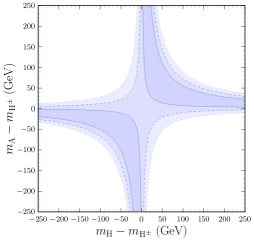
  (a) $(\Delta S,\Delta T)$ in eq. (22).

  

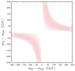
  (b) $(\Delta S,\Delta T)$ in eq. (23).

  

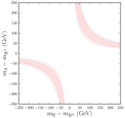
  (c) $(\Delta S,\Delta T)$ in eq. (24).

  Figure 1: Oblique parameters: allowed regions in $m_{\mathrm{A}}-m_{\mathrm{H}^{\pm}}$ vs. $m_{\mathrm{H}}-m_{\mathrm{H}^{\pm}}$. Darker to lighter colors correspond to 2D-$\Delta\chi^{2}$ 1, 2 and 3$\sigma$ regions. The plot corresponds to $m_{\mathrm{H}^{\pm}}=1$ TeV and scalar alignment.

• $\mathrm{H}^{\pm}$-induced FCNC. The charged scalar $\mathrm{H}^{\pm}$ can contribute to $\Delta F=1$ and $\Delta F=2$ FCNC processes like $b\to s\gamma$ and $B_{q}$–$\bar{B}_{q}$ mixings (for example, through SM-like box diagrams for $B_{q}$–$\bar{B}_{q}$ in which $W^{\pm}$ are replaced with $\mathrm{H}^{\pm}$). The dominant contributions involve virtual top quarks as in the SM, with couplings including now $t_{\beta}^{-1}$ factors. Keeping those contributions within experimental bounds only allows, roughly, the colored region in figure 2. For each value of $m_{\mathrm{H}^{\pm}}$ there is a lower bound on $t_{\beta}$. See [105, 106, 107] for further details.

  

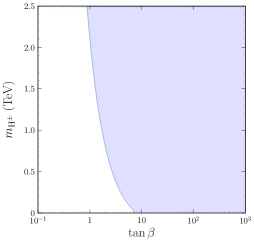
  Figure 2: $\mathrm{H}^{\pm}$ FCNC: $m_{\mathrm{H}^{\pm}}$ vs. $t_{\beta}$ allowed region when contributions of $\mathrm{H}^{\pm}$ to $B_{q}$–$\bar{B}_{q}$ are below experimental uncertainty in $\Delta M_{B_{q}}$.

• Scalar sector perturbativity. Additional constraints on scalar masses vs. $t_{\beta}$ arise from perturbativity requirements on the quartic coefficients of the scalar potential and from perturbative unitarity of $2\to 2$ scattering amplitudes [108, 109, 110, 111, 112, 113, 114]. With a $\mathbb{Z}_{2}$ symmetric potential, it is difficult to obtain masses above 1 TeV and values of $t_{\beta}$ larger than 8. Larger values of the masses and larger values of $t_{\beta}$ can be nevertheless obtained with the introduction of a soft symmetry breaking term $\mu_{12}^{2}\neq 0$ in eq. (4) [115, 114].

• Gluon-gluon fusion production cross section. Let us consider the production cross section of $\mathrm{H}$ and $\mathrm{A}$ through the one loop gluon-gluon fusion process. In the scalar alignment limit, one can read from eq. (20) that the same $t_{\beta}^{-1}$ factor applies to both pure scalar $\mathrm{H}$ and pure pseudoscalar $\mathrm{A}$ couplings with the top quark in the triangle loop:

  $$\sigma(pp\to S)_{\rm ggF}\propto t_{\beta}^{-2}|F_{S}(x)|^{2},\ x=4m_{t}^{2}/m_{S}^{2},\quad S=\mathrm{H},\mathrm{A}.$$ (25)

  The corresponding loop functions $F_{\mathrm{H}}$ and $F_{\mathrm{A}}$ [116, 117, 118, 119, 120, 121] are different due to the scalar or pseudoscalar character:

  $$F_{\mathrm{H}}(x)=-2x(1+(1-x)f(x)),$$ (26)

  $$F_{\mathrm{A}}(x)=-2xf(x),$$

  $$\quad f(x)=\left\{\begin{aligned} &\arcsin^{2}(1/\sqrt{x}),\quad&&x\geq 1\\ &-\frac{1}{4}\left(\ln\left(\frac{1+\sqrt{1-x}}{1-\sqrt{1-x}}\right)-i\pi\right)^{2},&&x<1\end{aligned}\right\}.$$

  Figure 3 shows $|F_{\mathrm{H}}(x)|^{2}$, $|F_{\mathrm{A}}(x)|^{2}$ and the ratio $|F_{\mathrm{A}}(x)|^{2}/|F_{\mathrm{H}}(x)|^{2}$ as a function of the scalar mass. It is clear that the pseudoscalar $\mathrm{A}$ has a larger gluon-gluon production cross section than the scalar $\mathrm{H}$ for $m_{\mathrm{A}}=m_{\mathrm{H}}$ (up to a factor of 6 for $m_{\mathrm{A}}=m_{\mathrm{H}}=2m_{t}$). Since dimuon searches $[pp]_{\rm ggF}\to S\to\mu^{+}\mu^{-}$ at the LHC can be rather constraining for scalar masses $m_{\rm S}<1$ TeV, one can expect that in that low mass region $m_{\mathrm{A}}>m_{\mathrm{H}}$. One could have worried about the validity of this expectation in case $\text{Br}\left(\mathrm{A}\to\mu^{+}\mu^{-}\right)\ll\text{Br}\left(\mathrm{H}\to\mu^{+}\mu^{-}\right)$, but the only way to achieve a suppression of $\text{Br}\left(\mathrm{A}\to\mu^{+}\mu^{-}\right)$ relative to $\text{Br}\left(\mathrm{H}\to\mu^{+}\mu^{-}\right)$ is through the existence of $\mathrm{A}\to\mathrm{H}Z$ decays, which are only available if $m_{\mathrm{A}}>m_{\mathrm{H}}$, and thus cannot change that expectation.

  

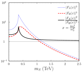
  Figure 3: Loop functions controlling gluon-gluon production cross sections of scalars.

• $e^{+}e^{-}\to\mu^{+}\mu^{-}$ at LEP. Sizable $n_{e}$ and $n_{\mu}$ are necessary ingredients for the contributions to $a_{e}$ and $a_{\mu}$ involving the new scalars $\mathrm{H}$, $\mathrm{A}$ and $\mathrm{H}^{\pm}$. Data from LEP [122] on $e^{+}e^{-}\to\mu^{+}\mu^{-}$ with $\sqrt{s}$ up to 210 GeV are sensitive to $s$-channel $\mathrm{H}$ and $\mathrm{A}$ mediated contributions (contrary to the LHC gluon-gluon fusion process, being scalar or pseudoscalar does not change the sensitivity of LEP data). One can roughly expect that agreement with LEP data imposes $m_{\mathrm{A}},m_{\mathrm{H}}\geq 210$ GeV.

4 Contributions to $\delta a_{\ell}$

The complete prediction of the anomalous magnetic moment $a_{\ell}^{\rm Th}$, $\ell=e,\mu$, is

$$a_{\ell}^{\rm Th}=a_{\ell}^{\rm SM}+\delta a_{\ell}\,,$$ (27)

where $a_{\ell}^{\rm SM}$ is the SM contribution and $\delta a_{\ell}$ the NP correction. The anomalies in eqs. (1)–(3) are “solved” for $\delta a_{e}=\delta a_{e}^{\rm Exp}$ and $\delta a_{\mu}=\delta a_{\mu}^{\rm Exp}$. We introduce for convenience $\Delta_{\ell}$ such that

$$\delta a_{\ell}=K_{\ell}\,\Delta_{\ell},\qquad K_{\ell}=\frac{1}{8\pi^{2}}\left(\frac{m_{\ell}}{v}\right)^{2}.$$ (28)

For $\delta a_{\mu}$ one needs

$$\Delta_{\mu}\simeq 1\,,$$ (29)

while for $\delta a_{e}$ one needs

$$\Delta_{e}^{\rm Cs}\simeq-16\,,\qquad\Delta_{e}^{\rm Rb}\simeq 9\,,$$ (30)

where the superscript corresponds to the different values in eqs. (2) and (3).

In the model considered here, it is well known that both one loop and two loop (of Barr-Zee type) contributions can be dominant. In this section we analyse both types of contributions in the scalar alignment limit $s_{\alpha\beta}\to 1$ and keeping only leading terms in $\frac{m_{\ell}^{2}}{m_{S}^{2}}$, ${S}=\mathrm{H},\mathrm{A},\mathrm{H}^{\pm}$. Full results, used for instance in the numerical analyses, can be found in appendix B.

4.1 One loop contributions to $\delta a_{\ell}$

The one loop result $\Delta_{\ell}^{(1)}$ has contributions from $\mathrm{H}$, $\mathrm{A}$ and $\mathrm{H}^{\pm}$. With the approximations mentioned above and the couplings in eqs. (20) and (21), we have

$$\Delta_{\ell}^{(1)}\simeq|n_{\ell}|^{2}\left(\frac{I_{\ell\mathrm{H}}}{m_{\mathrm{H}}^{2}}-\frac{I_{\ell\mathrm{A}}-2/3}{m_{\mathrm{A}}^{2}}-\frac{1}{6m_{\mathrm{H}^{\pm}}^{2}}\right)\,,$$ (31)

where

$$I_{\ell S}=-\frac{7}{6}-2\ln\left(\frac{m_{\ell}}{m_{S}}\right)\,.$$ (32)

The range of interest in our analyses will be $m_{S}\in[0.2;2.5]$ TeV, in which case

$$I_{\mu S}\in[13.9;18.9]\,,$$ (33)

while

$$I_{eS}=I_{\mu S}+2\ln\left(\frac{m_{\mu}}{m_{e}}\right)=I_{\mu S}+10.7\,.$$ (34)

In eq. (31), the $\mathrm{H}$ contribution is positive, the $\mathrm{A}$ contribution is negative and the $\mathrm{H}^{\pm}$ contribution is negligible. One can then anticipate the following.

• The muon anomaly $\Delta_{\mu}\simeq 1$ can only be explained with the one loop $\mathrm{H}$ contribution and provided

  $$1\simeq\frac{|n_{\mu}|^{2}}{m_{\mathrm{H}}^{2}}I_{\mu\mathrm{H}}\ \Rightarrow\ |n_{\mu}|\sim\frac{1}{4}m_{\mathrm{H}}\,.$$ (35)

  Considering $|n_{\mu}|<250$ GeV, a priori there could be a one loop explanation of $\delta a_{\mu}$ for $m_{\mathrm{H}}<1$ TeV. Since the $\mathrm{A}$ contribution has opposite sign, if $m_{\mathrm{A}}\sim m_{\mathrm{H}}$ a substantial cancellation would occur. As discussed in section 3, it is precisely for light $\mathrm{H}$ that one expects $m_{\mathrm{A}}>m_{\mathrm{H}}$, in which case that cancellation is largely avoided and a one loop $\mathrm{H}$ explanation viable. For heavier $m_{\mathrm{H}}$, the muon anomaly needs other contributions.

• For the electron ${\rm Cs}$ anomaly, $\Delta_{e}^{\rm Cs}\simeq-16$ can only be explained with the one loop $\mathrm{A}$ contribution provided

  $$-16\simeq-\frac{|n_{e}|^{2}}{m_{\mathrm{A}}^{2}}I_{e\mathrm{A}}\ \Rightarrow\ |n_{e}|\sim\frac{4}{5}m_{\mathrm{A}}\,.$$ (36)

  For $|n_{e}|<250$ GeV, this would require the pseudoscalar $\mathrm{A}$ to be rather light, $m_{\mathrm{A}}<300$ GeV. On the other hand, $m_{\mathrm{A}}>200$ GeV would require $|n_{e}|>160$ GeV: besides perturbativity concerns, such values of $|n_{e}|$ might be hard to reconcile with other constraints. More importantly, since we expect $m_{\mathrm{H}}<m_{\mathrm{A}}$ for light $\mathrm{A}$, we also expect a sizable cancellation among $\mathrm{H}$ and $\mathrm{A}$ contributions. From this simple analysis, obtaining $\Delta_{e}^{\rm Cs}\simeq-16$ with one loop contributions does not appear to be feasible.

• For the electron ${\rm Rb}$ anomaly, $\Delta_{e}^{\rm Rb}\simeq 9$ can only be explained with the one loop $\mathrm{H}$ contribution and provided

  $$9\simeq\frac{|n_{e}|^{2}}{m_{\mathrm{H}}^{2}}I_{e\mathrm{H}}\ \Rightarrow\ |n_{e}|\sim\frac{3}{5}m_{\mathrm{H}}\,.$$ (37)

  For $m_{\mathrm{H}}>200$ GeV, this would require $|n_{e}|>120$ GeV. If the same concerns on the values of $|n_{e}|$ mentioned for $\Delta_{e}^{\rm Cs}\simeq-16$ apply here, obtaining $\Delta_{e}^{\rm Rb}\simeq 9$ does not seem to be feasible neither; otherwise $\Delta_{e}^{\rm Rb}\simeq 9$ would be “easier” to accommodate with one loop contributions than $\Delta_{e}^{\rm Cs}\simeq-16$ because of the sign difference and the smaller absolute value.

4.2 Two loop contributions to $\delta a_{\ell}$

The dominant two loop contributions are the Barr-Zee ones. Diagrammatically they correspond to contributions where a closed fermion loop is attached to the external lepton through two propagators: one photon and one of the new scalars $\mathrm{H}$, $\mathrm{A}$. In the scalar alignment limit,

$$\Delta_{\ell}^{(2)}=-\frac{2\alpha}{\pi}\,\frac{\text{Re}\left(n_{\ell}\right)}{m_{\ell}}\,F\,.$$ (38)

It is important to notice that these contributions are linear in $n_{\ell}$. Detailed expressions are provided in appendix B. In eq. (38) we have

$$\frac{2\alpha}{\pi m_{e}}\simeq 9.1\,\text{GeV}^{-1},\qquad\frac{2\alpha}{\pi m_{\mu}}\simeq 0.044\,\text{GeV}^{-1}.$$ (39)

The function $F$ depends on the masses of the fermions in the closed loop, their couplings to $\mathrm{H}$ and $\mathrm{A}$, and on $m_{\mathrm{A}}$ and $m_{\mathrm{H}}$. Considering the dominant contributions from top and bottom quarks, and also from tau and muon leptons since $n_{\tau}$ and $n_{\mu}$ are free parameters,

$$F=\frac{t_{\beta}^{-1}}{3}\left[4(f_{t\mathrm{H}}+g_{t\mathrm{A}})+(f_{b\mathrm{H}}-g_{b\mathrm{A}})\right]+\frac{\text{Re}\left(n_{\tau}\right)}{m_{\tau}}(f_{\tau\mathrm{H}}-g_{\tau\mathrm{A}})+\frac{\text{Re}\left(n_{\mu}\right)}{m_{\mu}}(f_{\mu\mathrm{H}}-g_{\mu\mathrm{A}})\,,$$ (40)

with

$$f_{xS}=f\left(\frac{m^{2}_{x}}{m^{2}_{S}}\right),\quad g_{xS}=g\left(\frac{m^{2}_{x}}{m^{2}_{S}}\right)\,.$$ (41)

The functions $f(z)$ and $g(z)$ are defined in appendix B. It is to be noticed that (i) $f(z)\sim g(z)$ in the range of interest, (ii) larger values correspond to heavier fermions, (iii) for the top quark loop, $f$ and $g$ vary between $0.08$ and $1$ in the relevant range of scalar masses, $m_{S}\in[0.2;2.5]$ TeV.

• If the electron anomaly is to be obtained through the two loop contributions,

  $$\Delta_{e}\simeq-9.1\,F\,\text{Re}\left(n_{e}\right)/\text{GeV}\,,$$ (42)

  and thus

  $$\text{from }\Delta_{e}^{\rm Cs}\,,\quad\text{Re}\left(n_{e}\right)\,F\simeq 1.8\,\text{GeV}\,,$$ (43)

  $$\text{from }\Delta_{e}^{\rm Rb}\,,\quad\text{Re}\left(n_{e}\right)\,F\simeq-1.0\,\text{GeV}\,.$$

  The sign and the magnitude of $F$ is fixed by the $\text{Re}\left(n_{e}\right)$ value to fix $\delta a_{e}$.

• For $m_{\mathrm{H}}>1$ TeV, two loop contributions are necessary to explain the muon anomaly, in which case

  $$\Delta_{\mu}\simeq-0.044\,F\,\text{Re}\left(n_{\mu}\right)/\text{GeV}\ \Rightarrow\ \text{Re}\left(n_{\mu}\right)\,F\simeq-23\,\text{GeV}\,.$$ (44)

  If follows that, for $m_{\mathrm{H}}>1$ TeV,

  $$\text{for }\Delta_{e}^{\rm Cs}\text{ and }\Delta_{\mu}\,,\quad\text{Re}\left(n_{\mu}\right)\sim-13\text{Re}\left(n_{e}\right)\,,$$ (45)

  $$\text{for }\Delta_{e}^{\rm Rb}\text{ and }\Delta_{\mu}\,,\quad\text{Re}\left(n_{\mu}\right)\sim 23\text{Re}\left(n_{e}\right)\,.$$

These correlations show that, in the present framework, the independence of $n_{e}$ and $n_{\mu}$ is essential to explain the different sign of $\Delta_{e}^{\rm Cs}$ and $\Delta_{\mu}$. This sign difference is challenging for many scenarios addressing simultaneously both anomalies. In this sense, addressing $\Delta_{e}^{\rm Rb}$ and $\Delta_{\mu}$ is less challenging.

5 Analysis

In section 3 we have discussed some general constraints that apply without regard to the values of $n_{e}$ and $n_{\mu}$ of interest to reproduce the $\delta a_{\ell}$ anomalies; in section 4 we have explored the obtention of the $\delta a_{\ell}$ anomalies through one and two loop contributions. It is now time to present the main aspects of our detailed numerical analyses. The goal of the numerical analyses is to explore the parameter space of the model and map the different regions where a chosen set of relevant constraints is satisfied and the $\delta a_{\ell}$ anomalies are explained in terms of the new contributions. The independent parameters of the model are $\{t_{\beta},m_{\mathrm{H}},m_{\mathrm{A}},m_{\mathrm{H}^{\pm}},\mu_{12}^{2},c_{\alpha\beta},\text{Re}\left(n_{e}\right),\text{Re}\left(n_{\mu}\right),\text{Re}\left(n_{\tau}\right)\}$: $\{t_{\beta},m_{\mathrm{H}},m_{\mathrm{A}},m_{\mathrm{H}^{\pm}},\mu_{12}^{2},c_{\alpha\beta}\}$ control the scalar sector (together with $v$ and $m_{\mathrm{h}}$) while $\{\text{Re}\left(n_{e}\right),\text{Re}\left(n_{\mu}\right),\text{Re}\left(n_{\tau}\right)\}$ give the lepton Yukawa couplings (quark Yukawa couplings are fixed by $t_{\beta}$). The set of relevant constraints includes the following.

• Boundedness from below of the scalar potential [123], perturbativity of quartic couplings and perturbative unitarity of high energy $2\to 2$ scattering in the scalar sector [110].

• Corrections to the oblique parameters $S$ and $T$ in agreement with electroweak precision data [97, 102].

• “Production $\times$ decay” predictions for $\mathrm{h}$ in agreement with Higgs signal strengths [124, 125, 126, 127, 128, 129, 130, 131, 132, 133, 134, 135, 136]. As already mentioned, this constraint forces the alignment limit in the scalar sector: in the analyses of section 6 one obtains indeed $c_{\alpha\beta}<3\times 10^{-3}$.

• Lepton flavor universality in leptonic and semileptonic decays [97, 137, 138].

• $b\to s\gamma$ and $B_{q}^{0}$–$\bar{B}_{q}^{0}$ data [97, 105, 106].

• $e^{+}e^{-}\to\mu^{+}\mu^{-}$, $\tau^{+}\tau^{-}$ data from LEP (with center of mass energies up to 210 GeV) [122].

• LHC searches: resonant $pp\to S\to\mu^{+}\mu^{-},\tau^{+}\tau^{-}$ searches with gluon-gluon fusion $pp\to S$ production [139, 140, 141, 142, 143] and $\mathrm{H}^{\pm}$ searches in $pp\to\mathrm{H}^{\pm}tb$, $\mathrm{H}^{\pm}\to\tau\nu,tb$ [144, 145, 146, 147].

For additional details on the different constraints we refer to [41]. The constraints are typically modelled with a gaussian likelihood or an equivalent $\chi^{2}$ term, the overall likelihood is sampled over parameter space using Markov chain Monte Carlo techniques in order to obtain the regions where (best) agreement with the constraints is obtained. There are two final aspects of central importance which require a specific discussion: (i) how are the anomalies included in the analyses, (ii) what ranges are considered for the $n_{\ell}$ parameters.
Concerning the $a_{\ell}$ anomalies, the situation for $\delta a_{\mu}^{\rm Exp}$ is clear: one should consider eq. (1). On the contrary, for $\delta a_{e}^{\rm Exp}$ the situation is not settled: we have eq. (2) and eq. (3), which are rather incompatible. In order to have a complete picture, we analyse both cases separately. Furthermore, we also consider two additional possibilities concerning $\delta a_{e}^{\rm Exp}$:

• despite the marginal compatibility of $\delta a_{e}^{\rm Exp,Cs}$ and $\delta a_{e}^{\rm Exp,Rb}$, we combine them into

  $$\delta a_{e}^{\rm Exp,Avg}=-(2.0\pm 2.2)\times 10^{-13},$$ (46)

  which has the same sign as $\delta a_{e}^{\rm Exp,Cs}$, i.e. opposite to $\delta a_{\mu}^{\rm Exp}$, but a size close to 4 times smaller;

• a conservative approach in which we only assume that $|\delta a_{e}|\leq 20\times 10^{-13}$. Rather than targeting a specific value, this analysis may help to single out regions of parameter space where one cannot reproduce $\delta a_{\mu}^{\rm Exp}$ together with any value of $\delta a_{e}$ compatible with $\delta a_{e}^{\rm Exp,Cs}$ or $\delta a_{e}^{\rm Exp,Rb}$.

We will refer to these separate analyses as “$a_{e}^{\rm Cs}$”, “$a_{e}^{\rm Rb}$”, “$a_{e}^{\rm Avg}$”, “$a_{e}^{\rm Bound}$”. For their implementation in the analyses, we assign a joint $\chi^{2}$ contribution (corresponding to a gaussian factor in the likelihood)

$$\chi^{2}_{g-2}(\delta a_{e},\delta a_{\mu})=\left(\frac{\delta a_{e}-c_{e}}{s_{e}}\right)^{2}+\left(\frac{\delta a_{\mu}-c_{\mu}}{s_{\mu}}\right)^{2}\,,$$ (47)

where $c_{\ell}$ is the experimental central value and $s_{\ell}$ is the experimental uncertainty divided by 4. The scope of this choice – dividing the experimental uncertainty by 4 instead of simply using the experimental uncertainty – is to show clearly that the model can reproduce easily and simultaneously both the muon and the electron anomalies, and to guarantee that we are definitely reproducing a sizable deviation from the SM both in $a_{\mu}$ and in all cases for $a_{e}$, except the “$a_{e}^{\rm Bound}$” analysis where there is no $\delta a_{e}$ term in eq. (47) and $|\delta a_{e}|\leq 20\times 10^{-13}$ is imposed. As a summary, all four selected cases of $\delta a_{\mu}^{\rm Exp}$ vs. $\delta a_{e}^{\rm Exp}$ are represented in figure 4.

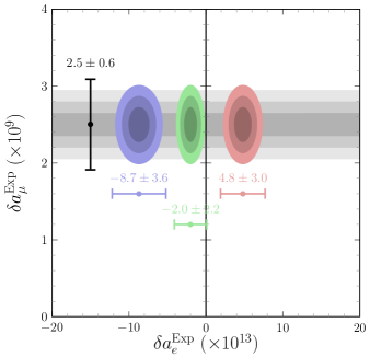
Figure 4: Allowed $\delta a_{\mu}^{\rm Exp}$ vs. $\delta a_{e}^{\rm Exp}$ regions in the different analyses.

The different colored regions in figure 4 represent three contours in the joint $\Delta\chi^{2}=\chi^{2}-\chi^{2}_{\rm{Min}}$ considering only eq. (47). In a 2D-$\Delta\chi^{2}$ distribution they correspond, darker to lighter, to 1, 2 and 3$\sigma$ regions with 68.2% C.L., 95.4% C.L. and 99.7% C.L., respectively. The same color coding is used in the figures below illustrating the final results of the analyses, where all observables and constraints have been included.
Finally, in [41], only $|n_{\ell}|\leq 100$ GeV were considered. Although for $|n_{e}|,|n_{\mu}|\sim 100$ GeV lepton couplings to the new scalars are hugely enhanced with respect to $\mathrm{h}$ couplings, it is true that $\frac{|n_{\ell}|}{v}\sim\frac{100\text{ GeV}}{v}\sim 0.4$ does not appear to pose a perturbativity challenge. In fact, the one loop correction to the imaginary part of the $m_{\mathrm{H}}$ mass is controlled by $\Gamma(\mathrm{H}\to\ell\bar{\ell})$ and the relevant ratio is $\frac{\Gamma}{m_{\mathrm{H}}}=\frac{1}{8\pi}\frac{|n_{\ell}|^{2}}{v^{2}}$, therefore arriving to $|n_{\ell}|=v\sim 250$ GeV represents one loop corrections at the 4% level. For this reason the analyses have been done with $|n_{\ell}|\leq 250$ GeV $\sim v$; furthermore, the analysis “$a_{e}^{\rm Cs}$” has been conducted both with $|n_{\ell}|\leq 100$ GeV (since this case is the closest one to [41]) and with $|n_{\ell}|\leq 250$ GeV.

6 Results

In the next subsections we discuss the most relevant results of the analyses done following the lines of the previous section. In subsection 6.1 we consider the scenario “$a_{e}^{\rm Cs}$” when $|n_{\ell}|\leq 100$ GeV is imposed. The implications of changing this last assumption to $|n_{\ell}|\leq 250$ GeV are addressed in subsection 6.2. The implications of the different assumptions for the electron anomaly, that is scenarios “$a_{e}^{\rm Rb}$”, “$a_{e}^{\rm Avg}$” and “$a_{e}^{\rm Bound}$” are explored in subsection 6.3. The impact of the recent measurement of $M_{W}$ by the CDF collaboration is considered in subsection 6.4. Finally, to further illustrate these discussions, a few complete example cases are shown in subsection 6.5.

6.1 $|n_{\ell}|\leq 100$ GeV

Here we present the results of the analysis “$a_{e}^{\rm Cs}$” with the perturbativity constraint $|n_{\ell}|\leq 100$ GeV. This serves to revisit the main results of [41] and as a reference for the analysis with $|n_{\ell}|\leq 250$ GeV addressed in the following subsection.

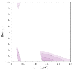
(a) $\text{Re}\left(n_{\mu}\right)$ vs. $m_{\mathrm{H}}$.

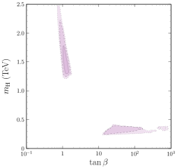
(b) $m_{\mathrm{H}}$ vs. $t_{\beta}$.

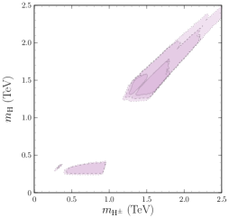
(c) $m_{\mathrm{H}}$ vs. $m_{\mathrm{H}^{\pm}}$.

Figure 5: Allowed regions: relevant correlations involving $m_{\mathrm{H}}$ with $|n_{\ell}|\leq 100$ GeV.

The perturbativity constraint limits the possibility of explaining $\delta a_{e}^{\rm Exp,Cs}$ via the one loop contribution, since it requires $m_{\mathrm{A}}\leq 125$ GeV for $|n_{e}|\leq 100$ GeV (see eq. (36)) which is not allowed by $e^{+}e^{-}\to\mu^{+}\mu^{-}$ LEP data. On that respect, lepton flavor universality constraints also limit the possibility of a one loop explanation for the electron anomaly, as discussed later. This leaves us with two scenarios, one where both anomalies are explained via the two loop contribution, following the scaling law in eq. (45), and another where the muon anomaly is one loop dominated while the electron one is still generated at two loops.
In figure 5a the allowed regions for $\text{Re}\left(n_{\mu}\right)$ are presented as a function of $m_{\mathrm{H}}$. Three disjoint regions in the scalar mass can be seen: two in the 200-400 GeV range and the other above 1.2 TeV. The low mass regions belong to the scenario where the muon anomaly is obtained through the one loop contribution in agreement with the relation in eq. (35). Note that this contribution depends on the absolute value of the coupling, so both signs are allowed for $\text{Re}\left(n_{\mu}\right)$. In the large mass region both leptonic anomalies are two loop dominated.
Figure 5b shows $m_{\mathrm{H}}$ vs. $t_{\beta}$. It contains two separate allowed regions again: in the $t_{\beta}\sim 1$ regime only scalar masses above 1.2 TeV are allowed; conversely for $t_{\beta}$ larger than 10, $m_{\mathrm{H}}$ lies in the 200-400 GeV interval.
To complement the previous two plots, in figure 5c the relation between the masses $m_{\mathrm{H}}$ and $m_{\mathrm{H}^{\pm}}$ is shown. In the low mass region we can clearly distinguish two scenarios. One where $m_{\mathrm{H}^{\pm}}\simeq m_{\mathrm{H}}$ and another where $m_{\mathrm{H}^{\pm}}>m_{\mathrm{H}}$; in the latter, $m_{\mathrm{H}^{\pm}}\simeq m_{\mathrm{A}}$.The degeneracy of $\mathrm{H}^{\pm}$ with either $\mathrm{H}$ or $\mathrm{A}$ arises from the oblique parameters constraint, as mentioned in section 3. In the large mass region the mass differences do not exceed $\pm 300$ GeV.

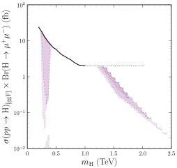
(a) For $S=\mathrm{H}$.

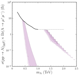
(b) For $S=\mathrm{A}$.

Figure 6: $\sigma(pp\to S)_{\rm[ggF]}\times\text{Br}\left(S\to\mu^{+}\mu^{-}\right)$ vs. $m_{S}$ allowed regions with $|n_{\ell}|\leq 100$ GeV.

Figure 6 illustrates the allowed regions for the resonant process $[pp]_{\rm{ggF}}\to S\to\mu^{+}\mu^{-}$ with respect to the scalar mass $m_{S}$ for $S=\mathrm{H},\mathrm{A}$. The black line corresponds to the limit observed by CMS [140]. Although LHC direct searches are already constraining the allowed regions, there is ample room for extra scalars that can explain both $g-2$ anomalies simultaneously.

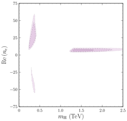
(a) $\text{Re}\left(n_{e}\right)$ vs. $m_{\mathrm{H}}$.

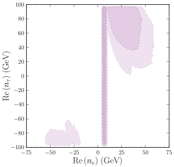
(b) $\text{Re}\left(n_{\tau}\right)$ vs. $\text{Re}\left(n_{e}\right)$.

Figure 7: Allowed regions for $\text{Re}\left(n_{e}\right)$ with $|n_{\ell}|\leq 100$ GeV.

Let us now discuss some results concerning $\text{Re}\left(n_{e}\right)$ and $\text{Re}\left(n_{\tau}\right)$. With a two loop explanation of the electron anomaly, it follows from eqs. (38) and (40) (see appendix B for further details) that one could have expected that both the coupling $\text{Re}\left(n_{e}\right)$ and the deviation $\delta a_{e}$ have opposite sign: this is confirmed in figure 7 in the 1$\sigma$ region. However, this figure also contains regions where $\text{Re}\left(n_{e}\right)$ is negative. This behavior might be understood by analysing with some detail the two loop contribution to $\delta a_{e}$: $F$ in eq. (40) can be decomposed as $F=F_{q}+F_{\tau}+F_{\mu}$, where $F_{f}$ is the contribution with fermion $f$ running in the closed loop. One can estimate the importance of the different contributions for different $t_{\beta}$, $m_{\mathrm{H}}$ and $m_{\mathrm{A}}$ ranges.

• For $t_{\beta}\sim 1$ and $m_{\mathrm{H}},m_{\mathrm{A}}>1.2$ TeV, eq. (40) gives

  $$F_{q}>0.18\,,\quad\left|F_{\tau}\right|<0.13\times 10^{-4}\frac{\text{Re}\left(n_{\tau}\right)}{1\text{ GeV}}\,,\quad\left|F_{\mu}\right|<0.12\times 10^{-5}\frac{\text{Re}\left(n_{\mu}\right)}{1\text{ GeV}}\,.$$ (48)

  It is clear that in this region the quark-induced contribution $F_{t}$ is (i) necessarily dominant and (ii) it requires $\text{Re}\left(n_{e}\right)\sim 4-10$ GeV, as figure 7a illustrates, in order to reproduce $\Delta_{e}^{\rm Cs}\simeq-16$.

• For $t_{\beta}>10$, $m_{\mathrm{H}}\in[200,400]$ GeV and $m_{\mathrm{A}}\in[400,1000]$ GeV, eq. (40) gives

  $$F_{q}<0.18\,,\quad F_{\tau}\in[0.02,0.15]\times 10^{-2}\frac{\text{Re}\left(n_{\tau}\right)}{1\text{ GeV}}\,,\quad F_{\mu}\in[0.04,0.25]\times 10^{-3}\frac{\text{Re}\left(n_{\mu}\right)}{1\text{ GeV}}\,.$$ (49)

  In this case, large values of $\text{Re}\left(n_{\tau}\right)\simeq\pm 100$ GeV give $\tau$-induced contributions at the same level of, or even larger than, the quark-induced contribution. This occurs despite some cancellation among the $\tau\mathrm{H}$ and $\tau\mathrm{A}$ contributions in eq. (40). This scenario would require $\text{Re}\left(n_{e}\right)\lesssim-15$ GeV or $\text{Re}\left(n_{e}\right)\gtrsim 7$ GeV, as shown in figure 7a, in order to reproduce $\Delta_{e}^{\rm Cs}\simeq-16$.

From this simple estimates one can conclude that, besides the expected regions where $\delta a_{e}$ arises from quark-induced two loop contributions, regions where the $\tau$-induced contributions have an important role might be present. For this to occur, one might expect some peculiarities: besides light $\mathrm{H}$ and large $t_{\beta}$, large values of both $|\text{Re}\left(n_{\tau}\right)|$ and $|\text{Re}\left(n_{e}\right)|$, with $\text{Re}\left(n_{\tau}\right)$ and $\text{Re}\left(n_{e}\right)$ having the same sign, are required. Contrary to the case with dominating quark induced contributions, one might then have allowed regions where $\text{Re}\left(n_{e}\right)<0$. This is illustrated in figures 7a and 7b where one can observe how allowed $\text{Re}\left(n_{e}\right)<0$ only appear for a light $\mathrm{H}$, and how the regions with large $\pm\text{Re}\left(n_{e}\right)$ correspond to large $\pm\text{Re}\left(n_{\tau}\right)$.

To close this subsection, it is worth analysing in detail the role of the lepton flavor universality constraints mentioned in section 5. As justified later, we focus on observables involving only $\mu$’s and $e$’s. For the ratios

$$R_{\mu e}^{P}=\frac{\Gamma(P^{+}\to\mu^{+}\nu)}{\Gamma(P^{+}\to\mu^{+}\nu)_{\rm SM}}\frac{\Gamma(P^{+}\to e^{+}\nu)_{\rm SM}}{\Gamma(P^{+}\to e^{+}\nu)}\,,$$ (50)

the current constraints are [97]

$$R_{\mu e}^{\pi}=1+(4.1\pm 3.3)\times 10^{-3}\,,\qquad R_{\mu e}^{K}=1-(4.8\pm 4.7)\times 10^{-3}\,.$$ (51)

In the present scenario,

$$R_{\mu e}^{P}=\frac{|1-\Delta_{\mu}^{P}|^{2}}{|1-\Delta_{e}^{P}|^{2}}\,,\qquad|1-\Delta_{\ell}^{P}|^{2}=\left|1-\frac{M_{P}^{2}}{t_{\beta}m_{\mathrm{H}^{\pm}}^{2}}\frac{\text{Re}\left(n_{\ell}\right)}{m_{\ell}}\right|^{2}\,,$$ (52)

and thus, for $\Delta_{\ell}^{P}\ll 1$,

$$R_{\mu e}^{P}\simeq 1+2\frac{M_{P}^{2}}{t_{\beta}m_{\mathrm{H}^{\pm}}^{2}}\left(\frac{\text{Re}\left(n_{e}\right)}{m_{e}}-\frac{\text{Re}\left(n_{\mu}\right)}{m_{\mu}}\right)\,.$$ (53)

The presence of $M_{P}^{2}$ and the lepton masses allows us to concentrate on $R_{\mu e}^{K}$ and neglect the $n_{\mu}$ contribution. Therefore from eq. (51) we get the constraint

$$\text{Re}\left(n_{e}\right)<5\frac{t_{\beta}m_{\mathrm{H}^{\pm}}^{2}}{1\text{ TeV}^{2}}\text{ GeV}\,.$$ (54)

Then,

• for $t_{\beta}\simeq 1$ and $m_{\mathrm{H}^{\pm}}\simeq 2$ TeV, $\text{Re}\left(n_{e}\right)<20$ GeV,

• while for $t_{\beta}\simeq 10^{2}$ and $m_{\mathrm{H}^{\pm}}\simeq 0.5$ TeV, $\text{Re}\left(n_{e}\right)<125$ GeV.

From muon decay constraints on the $\mathrm{H}^{\pm}$ mediated contributions we also have a $t_{\beta}$ independent constraint (since the process is purely leptonic) [97, 107]:

$$\left|\frac{n_{e}n_{\mu}}{m_{\mathrm{H}^{\pm}}^{2}}\right|<0.035\,.$$ (55)

This constraint is relevant for the low mass region: for $\text{Re}\left(n_{\mu}\right)\simeq 100$ GeV, we can rewrite

$$|n_{e}|<87\left(\frac{m_{\mathrm{H}^{\pm}}}{0.5\text{ TeV}}\right)^{2}\text{ GeV}\,,$$ (56)

which is more restrictive than the bound from $R_{\mu e}^{K}$ above. Concerning other observables involving $\tau$ leptons, semileptonic processes are not sensitive to $n_{\tau}$ due to $\frac{m_{e}}{m_{\tau}}$ and $\frac{m_{\mu}}{m_{\tau}}$ suppressions, while purely leptonic decays have looser bounds than eq. (55).
This simple numerical exercise confirms that $\delta a_{e}^{\rm Exp}$ cannot be explained through one loop contributions.

6.2 $|n_{\ell}|\leq 250$ GeV

As previously motivated, perturbativity bounds on the Yukawa couplings should be studied in detail. Here we explore higher scales in $n_{\ell}$, namely changing from $|n_{\ell}|\leq 100\ \rm{GeV}$ to $|n_{\ell}|\leq 250\ \rm{GeV}$ while maintaining the same constraints of the previous section. Conversely to what one would naively expect, it is not just the allowed regions in the different $n_{\ell}$ that might change, but it has direct consequences on other physical observables such as the scalar masses and $t_{\beta}$, among others.

Figure 8a shows results for $\text{Re}\left(n_{\mu}\right)$ vs. $m_{\mathrm{H}}$. It is clear that the allowed regions in parameter space are notably enlarged with respect to those in figure 5a, which are completely embedded in the ones of this new analysis, as one could have expected. On that respect, one may realize of the appearance of a new set of intermediate values for the scalar mass, $m_{\mathrm{H}}\in[0.4;1.2]\ \rm{TeV}$, when increasing our perturbativity upper bound. It can be easily understood by tracing an horizontal line at $\text{Re}\left(n_{\mu}\right)_{0}=-100$ GeV: we eliminate the blue region “bridge” connecting the low and high mass solutions. Therefore, this new range of scalar masses requires large values of $|\text{Re}\left(n_{\mu}\right)|$.

(a) $\text{Re}\left(n_{\mu}\right)$ vs. $m_{\mathrm{H}}$.

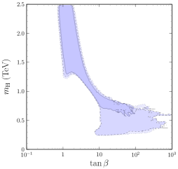
(b) $m_{\mathrm{H}}$ vs. $t_{\beta}$.

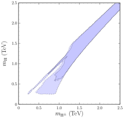
(c) $m_{\mathrm{H}}$ vs. $m_{\mathrm{H}^{\pm}}$.

Figure 8: Allowed regions: relevant correlations involving $m_{\mathrm{H}}$ with $|n_{\ell}|\leq 250$ GeV.

To fully characterize the impact of perturbativity on the allowed parameter space, figure 8b illustrates the scalar mass $m_{\mathrm{H}}$ in terms of $t_{\beta}$. Taking into account the appearance of new intermediate solutions in $m_{\mathrm{H}}$, one could expect that this behavior is translated into $t_{\beta}$. As figure 8b corroborates, new values of $t_{\beta}$, roughly in the range $1\leq t_{\beta}\leq 10$, are allowed when changing the perturbativity requirement from $|n_{\ell}|\leq 100$ GeV to $|n_{\ell}|\leq 250$ GeV. Furthermore, one may also notice by comparing with figure 5b that the top blue region for large $m_{\mathrm{H}}$ becomes wider, around a factor 2.5 in $t_{\beta}$ for each value of the scalar mass.

Figure 8c shows correlations among the scalar masses $m_{\mathrm{H}}$ and $m_{\mathrm{H}^{\pm}}$. Concerning the low mass regions where $\mathrm{H}^{\pm}$ is degenerate either with $\mathrm{H}$ or $\mathrm{A}$, already mentioned in figure 5c, it can be observed that enlarging perturbativity bounds pushes the upper limit of these regions in such a way that $m_{\mathrm{H}^{\pm}}\in[0.2;1.2]$ TeV for $m_{\mathrm{H}^{\pm}}\simeq m_{\mathrm{H}}$ and $m_{\mathrm{H}^{\pm}}\in[0.4;1.2]$ TeV for $m_{\mathrm{H}^{\pm}}\simeq m_{\mathrm{A}}$, to a high degree of accuracy. Figures 9a and 9b complete the results for the scalar masses. For instance, it is still true that $m_{\mathrm{A}}>m_{\mathrm{H}}$ in the low mass region, according to the general constraints presented in section 3.

(a) $m_{\mathrm{A}}$ vs. $m_{\mathrm{H}}$.

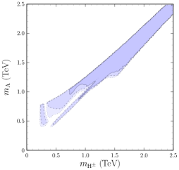
(b) $m_{\mathrm{A}}$ vs. $m_{\mathrm{H}^{\pm}}$.

Figure 9: Allowed regions for scalar masses with $|n_{\ell}|\leq 250$ GeV.

On the other hand, figure 10 shows the resonant process $[pp]_{\rm{ggF}}\to S\to\mu^{+}\mu^{-}$ as a function of the scalar mass $m_{S}$ for $S=\mathrm{H},\mathrm{A}$, which acquire an important role since we may be entering an era of exclusion or discovery at the LHC. As disclosed above, the existence of an intermediate set of solutions, $m_{\mathrm{H}}\in[0.4;1.2]$ TeV and $m_{\mathrm{A}}\in[0.9;1.2]$ TeV, opens the possibility to detect a sizeable signal in that range of scalar masses that was not contemplated in figure 6. Moreover, it is clear that increasing $|n_{\ell}|$ up to $|n_{\ell}|\leq 250$ GeV modifies our expectations for $\text{Br}\left(S\to\ell^{+}\ell^{-}\right)$ and, in particular, enlarges the allowed parameter space, as one can easily check.

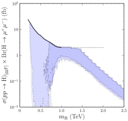
(a) For $S=\mathrm{H}$.

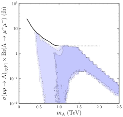
(b) For $S=\mathrm{A}$.

Figure 10: $\sigma(pp\to S)_{\rm[ggF]}\times\text{Br}\left(S\to\mu^{+}\mu^{-}\right)$ vs. $m_{S}$ allowed regions with $|n_{\ell}|\leq 250$ GeV.

Finally, we should stress some aspects concerning $\text{Re}\left(n_{e}\right)$ and $\text{Re}\left(n_{\mu}\right)$ from figure 11. In spite of increasing our perturbativity bound up to $|n_{\ell}|\leq 250$ GeV, it still seems difficult to obtain a one loop explanation for the electron anomaly since it requires quite large couplings, namely $|n_{e}|>160$ GeV in the Cs case. Figure 11b shows that $|n_{e}|<150$ GeV in the relevant range of scalar masses, thus indicating that $\delta a_{e}^{\rm Exp,Cs}$ is mainly explained at two loops. This agrees with the discussion on universality constraints closing subsection 6.1.
As it was already explained in the discussion of figure 7a, now in figure 11b and for large scalar masses, one can easily check that the electron coupling is positive and lies in the range $\text{Re}\left(n_{e}\right)\sim 4-20$ GeV. Furthermore, according to eq. (45), there exists a linear relation between $\text{Re}\left(n_{\mu}\right)$ and $\text{Re}\left(n_{e}\right)$ for $m_{\mathrm{H}}>1.2$ TeV, which implies that they have opposite sign in the Cs case and therefore $\text{Re}\left(n_{\mu}\right)$ should be negative in this region. The region $\text{Re}\left(n_{\mu}\right)=-13\text{Re}\left(n_{e}\right)$ can be seen in the lower part of figure 11a inside the 1$\sigma$ region as it should. Departure from this straight line introduces an important one loop contribution to the muon anomaly lowering also the scalar masses ranges. On the other hand, for light scalar masses, $\text{Re}\left(n_{e}\right)$ might be either positive or negative by the same arguments discussed in section 6.1. It is also important to recall that, in this low mass region, $\Delta_{\mu}$ receives dominant one loop contributions and thus $\text{Re}\left(n_{\mu}\right)$ could naturally appear with both signs. From figure 11a, one may notice as well that $|n_{\mu}|$ is in general larger than $|n_{e}|$ in the whole parameter space.

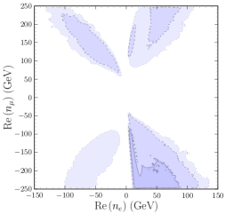
(a) $\text{Re}\left(n_{\mu}\right)$ vs. $\text{Re}\left(n_{e}\right)$.

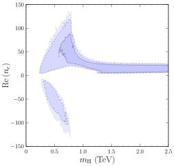
(b) $\text{Re}\left(n_{e}\right)$ vs. $m_{\mathrm{H}}$.

Figure 11: Allowed regions for $\text{Re}\left(n_{e}\right)$ with $|n_{\ell}|\leq 250$ GeV.

6.3 Different $\delta a_{e}$

As commented in section 5, the situation concerning $a_{e}$ is to some extent unclear. In this section we discuss the implications of different assumptions for the value of $\delta a_{e}^{\rm Exp}$, that is, in terms of the model, the implications of requiring different values of the new contributions $\delta a_{e}$. The ultimate answer is definitely provided by repeating detailed numerical analyses under the different assumptions $\delta a_{e}^{\rm Exp}$. However, one can anticipate part of the answer with simple considerations. As analysed in section 4, $\delta a_{e}$ arises from two loop contributions proportional to $\text{Re}\left(n_{e}\right)$: this fact, together with the results of section 6.2 corresponding to $\delta a_{e}\simeq\delta a_{e}^{\rm Exp,Cs}$, can give us a first insight. Consider for example an allowed point in parameter space (i.e. a point respecting all imposed constraints) which gives $\delta a_{e}\simeq\delta a_{e}^{\rm Exp,Cs}$. This point has a certain $\text{Re}\left(n_{e}\right)=\text{Re}\left(n_{e}\right)_{\rm Cs}$; it is straightforward that changing $\text{Re}\left(n_{e}\right)\mapsto\text{Re}\left(n_{e}\right)^{\prime}=\text{Re}\left(n_{e}\right)_{\rm Rb}=\text{Re}\left(n_{e}\right)_{\rm Cs}\times\frac{\delta a_{e}^{\rm Exp,Rb}}{\delta a_{e}^{\rm Exp,Cs}}$ and no other parameter, one would obtain $\delta a_{e}\simeq\delta a_{e}^{\rm Exp,Rb}$. The question is, of course, if such a change in $\text{Re}\left(n_{e}\right)$ alone still gives an allowed point. On that respect, one needs to analyse which observables constrain $\text{Re}\left(n_{e}\right)$ and how those constraints work. These are the ones related to lepton flavor universality in leptonic decays $\ell_{i}\to\ell_{j}\nu\bar{\nu}$ and in semileptonic decays involving kaons and pions, analysed in section 6.1. In particular, attending to $\delta a_{e}^{\rm Exp,Cs}$, $\delta a_{e}^{\rm Exp,Rb}$ and $\delta a_{e}^{\rm Exp,Avg}$ in eqs. (2), (3) and (46), one is interested in the effect on those constraints of

$$\text{Re}\left(n_{e}\right)=\text{Re}\left(n_{e}\right)_{\rm Cs}\mapsto\text{Re}\left(n_{e}\right)^{\prime}=\text{Re}\left(n_{e}\right)_{\rm Rb}=-0.55\text{Re}\left(n_{e}\right)_{\rm Cs}\,,$$ (57)

$$\text{Re}\left(n_{e}\right)=\text{Re}\left(n_{e}\right)_{\rm Cs}\mapsto\text{Re}\left(n_{e}\right)^{\prime}=\text{Re}\left(n_{e}\right)_{\rm Avg}=0.23\text{Re}\left(n_{e}\right)_{\rm Cs}\,,$$

when no other parameter is changed. There are two different aspects:

1. since $|\text{Re}\left(n_{e}\right)_{\rm Avg}|,|\text{Re}\left(n_{e}\right)_{\rm Rb}|<|\text{Re}\left(n_{e}\right)_{\rm Cs}|$, the constraint on $|n_{e}|$ from $\mu\to e\nu\bar{\nu}$ decays in eq. (56) is necessarily less restrictive when eq. (57) is considered;

2. besides the uncertainty in $R^{K}_{\mu e}$ in eq. (51), as discussed previously, there is a “sign” question concerning the deviation, at the same $\simeq 5\times 10^{-3}$ level of the uncertainty, from $R^{K}_{\mu e}=1$. In order to obtain $\delta a_{e}\simeq\delta a_{e}^{\rm Exp,Cs}<0$, the expectation is $\text{Re}\left(n_{e}\right)>0$, and that produces $R^{K}_{\mu e}-1>0$ in eq. (53), which goes “in the wrong direction”. For both cases in eq. (57), that problem is alleviated.

It is then clear that the analysis with $\delta a_{e}^{\rm Exp,Cs}$ is somehow a “worst case” scenario in terms of the dependence of the constraints on $\text{Re}\left(n_{e}\right)$: besides the naive mapping of allowed regions expected from eq. (57), one might then expect larger allowed regions not only for $\text{Re}\left(n_{e}\right)$ but also for other quantities of interest. As mentioned in section 5, we also perform an analysis where $|\delta a_{e}|\leq 20\times 10^{-13}$ is imposed (instead of requiring some specific value, as summarized in figure 4). This serves a double purpose: identifying which allowed regions are necessary in order to obtain an appropriate $\delta a_{\mu}$ without regard to $\delta a_{e}$, and identifying which regions are absolutely excluded for any value of $\delta a_{e}$ reasonably compatible with $\delta a_{e}^{\rm Exp,Cs}$ or $\delta a_{e}^{\rm Exp,Rb}$ that one could consider.
In figures 12, 13 and 14, the color coding follows figure 4. Figure 12 shows $\text{Re}\left(n_{\mu}\right)$ vs. $\text{Re}\left(n_{e}\right)$ and $\text{Re}\left(n_{e}\right)$ vs. $m_{\mathrm{H}}$ allowed regions: comparison with figures 11a and 11b confirms the simple expectations of the previous discussion in terms of the position of the allowed regions and their extension. The same applies to figure 13, which shows $\text{Re}\left(n_{\mu}\right)$ vs. $m_{\mathrm{H}}$ (to be compared with figure 8a). In particular it is clear from figure 13c that once $\delta a_{\mu}\simeq\delta a_{\mu}^{\rm Exp}$ is imposed, the allowed regions for some parameters (besides $\text{Re}\left(n_{\mu}\right)$, obviously) are coarsely determined and the sensitivity of the analysis on the requirement for $\delta a_{e}$ only concerns a finer level of detail.

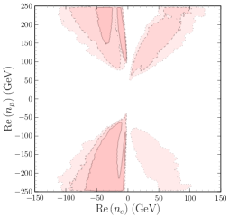
(a)

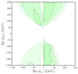
(b)

(c)

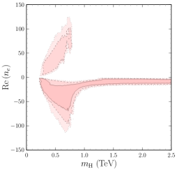
(d)

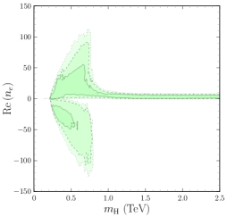
(e)

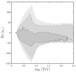
(f)

Figure 12: $\text{Re}\left(n_{e}\right)$ correlations.

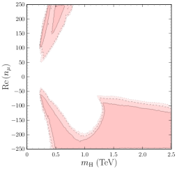
(a)

(b)

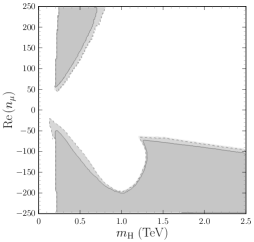
(c)

Figure 13: $\text{Re}\left(n_{\mu}\right)$ vs. $m_{\mathrm{H}}$ correlations.

There is a final point that the analysis with $|\delta a_{e}|\leq 20\times 10^{-13}$ confirms. Figure 14 shows $\delta a_{e}$ vs. $\text{Re}\left(n_{e}\right)$: under the simple expectations for the two loop contributions discussed in section 4.2, one would have $\text{Re}\left(n_{e}\right)\times\delta a_{e}<0$. Besides that expected region, one can observe smaller allowed regions where $\text{Re}\left(n_{e}\right)\times\delta a_{e}>0$: they correspond to the unexpected situation in which the two loop contributions are dominated by virtual $\tau$’s in the fermion loop, and furthermore it is clear that the values of $\delta a_{e}$ that can be obtained in this manner are more restricted, with $|\delta a_{e}|<10^{-12}$.

Figure 14: $\delta a_{e}$ vs. $\text{Re}\left(n_{e}\right)$.

6.4 The CDF $M_{W}$ anomaly

As mentioned in section 3, one can use deviations from the SM in the oblique parameters $(\Delta S,\Delta T)\neq(0,0)$ in order to “explain” the CDF measurement of $M_{W}$ in [96]: this subsection is devoted to that “explanation”. Figures 15 and 16 show results analogous to the ones in section 6.2 –which use eq. (22)–, except for a different $(\Delta S,\Delta T)$ constraint. Figure 15 is obtained with eq. (23) (the “conservative” average of [103]) and figure 16 is obtained with eq. (24) (the results in [104]). The coloring of the allowed regions corresponds, darker to lighter, to $1,2,3\sigma$ levels of a 2D-$\Delta\chi^{2}$. For $\Delta\chi^{2}$ we use the $\chi^{2}_{\rm Min}$ value of the analysis in section 6.2 (that is, with the constraint in eq. (22) for $\Delta S$, $\Delta T$). A few comments are in order.

• Besides the absence of degeneracies $m_{\mathrm{H}^{\pm}}\simeq m_{\mathrm{H}}$ or $m_{\mathrm{H}^{\pm}}\simeq m_{\mathrm{A}}$, masses of the new scalars larger than 2 TeV are more difficult to accommodate. This can be understood attending to the clash between the mass differences discussed in section 3 that eqs. (23) or (24) require, and the need of near degenerate scalars that the perturbativity requirements on the scalar potential impose for new scalar masses much larger than $v$.

• Overall agreement with the imposed constraints is worse in several regions in figures 15 and 16 than it was in the analyses of section 6.2 (figures 8, 9 and 11). This is more dramatic in figure 16, where the agreement with constraints is worse than in figure 15 to the point that several regions are beyond the represented contour levels.

Despite these changes, the main characteristics of the allowed regions discussed in the previous sections still apply and are clearly identified in both figures 15 and 16.

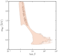
(a) $m_{\mathrm{H}}$ vs. $t_{\beta}$.

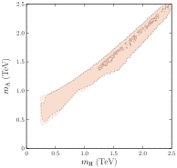
(b) $m_{\mathrm{A}}$ vs. $m_{\mathrm{H}}$.

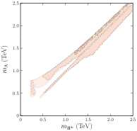
(c) $m_{\mathrm{A}}$ vs. $m_{\mathrm{H}^{\pm}}$.

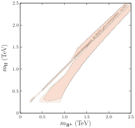
(d) $m_{\mathrm{H}}$ vs. $m_{\mathrm{H}^{\pm}}$.

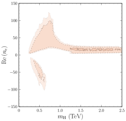
(e) $\text{Re}\left(n_{e}\right)$ vs. $m_{\mathrm{H}}$.

(f) $\text{Re}\left(n_{\mu}\right)$ vs. $m_{\mathrm{H}}$.

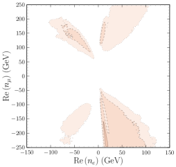
(g) $\text{Re}\left(n_{\mu}\right)$ vs. $\text{Re}\left(n_{e}\right)$.

Figure 15: Results with $(\Delta S,\Delta T)$ in eq. (23), “conservative” case in [103].

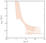
(a) $m_{\mathrm{H}}$ vs. $t_{\beta}$.

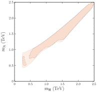
(b) $m_{\mathrm{A}}$ vs. $m_{\mathrm{H}}$.

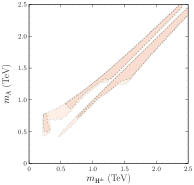
(c) $m_{\mathrm{A}}$ vs. $m_{\mathrm{H}^{\pm}}$.

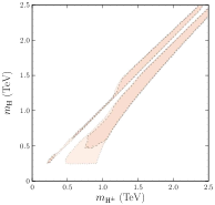
(d) $m_{\mathrm{H}}$ vs. $m_{\mathrm{H}^{\pm}}$.

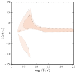
(e) $\text{Re}\left(n_{e}\right)$ vs. $m_{\mathrm{H}}$.

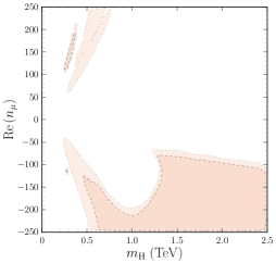
(f) $\text{Re}\left(n_{\mu}\right)$ vs. $m_{\mathrm{H}}$.

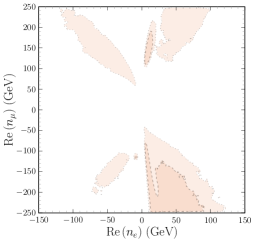
(g) $\text{Re}\left(n_{\mu}\right)$ vs. $\text{Re}\left(n_{e}\right)$.

Figure 16: Results with $(\Delta S,\Delta T)$ in eq. (24), from [104].

Finally, since the oblique parameters $S$ and $T$ play an important role, figure 17 shows allowed regions for $\Delta S$ vs. $\Delta T$ in the two scenarios considered for the CDF $M_{W}$ “explanation”, together with the imposed $(\Delta T,\Delta S)$ constraint in each case. As anticipated, the constraint in eq. (24) appears to be more difficult to accommodate than the constraint in eq. (23). In fact, despite the different position of the ellipses corresponding to the $(\Delta T,\Delta S)$ constraints in figures 17a and 17b, the allowed regions are quite similar in both cases, that is, the model appears to be unable to accommodate values $\Delta T>0.22$ together with $\Delta S>0.02$. Other possible explanations of the CDF $M_{W}$ anomaly have been addressed in [148, 149, 150, 151, 152, 153, 154, 155].

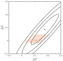
(a) $(\Delta S,\Delta T)$ in eq. (23).

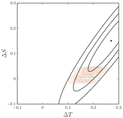
(b) $(\Delta S,\Delta T)$ in eq. (24).

Figure 17: $\Delta S$ vs. $\Delta T$, 1, 2 and 3$\sigma$ 2D-$\Delta\chi^{2}$ contours from the imposed constraint are shown together with the allowed regions.

6.5 Example points

In this section, some example points of the allowed parameter space are presented in order to specify the behavior pointed out in the previous plots. For the sake of clarity, we only focus on the analysis with “$a_{e}^{\rm Cs}$” concerning the electron anomaly: other cases do not change substantially beyond the differences already mentioned in section 6.3.

From table 1, it is clear that points 1–2 correspond to the solution with small values of $t_{\beta}$ and large scalar masses: all scalars are above $1.2\ \rm{TeV}$ and their mass differences do not exceed $\pm 200$ GeV. In this region, both anomalies are explained at two loops through the top quark terms, as one can easily check in tables 2 and 3, where all loop contributions are normalized to the total $\delta a_{\ell}$ in such a way that their sum must be 1. One may also notice that $\delta a_{\mu}$ receives a subdominant one loop contribution. The lepton couplings $\text{Re}\left(n_{e}\right)$ and $\text{Re}\left(n_{\mu}\right)$ have opposite sign and they roughly satisfy the linear relation in eq. (45) for the Cs case.

Regarding the appearance of the intermediate values of the scalar masses and $t_{\beta}$ previously commented in section 6.2, our point 3 gives a perfect example of that behavior. It is important to realize that large values of $|\text{Re}\left(n_{\mu}\right)|$ are required in this region; in fact, they are almost reaching the perturbativity upper bound $|n_{\ell}|\leq 250$ GeV. On the other hand, although the top dominance still holds at two loops in the electron anomaly, the corresponding tau contributions begin to play a relevant role. This trend will continue as $t_{\beta}$ grows and the quark contributions are more suppressed.

Finally, points 4–9 belong to the low mass region corresponding to a wide range of $t_{\beta}\gg 1$ values. As we have stressed before, two possible scenarios arise: one where $m_{\mathrm{H}^{\pm}}\simeq m_{\mathrm{A}}$ (points 4–6) and another where $m_{\mathrm{H}^{\pm}}\simeq m_{\mathrm{H}}$ (points 7–9). In all cases, the scalar masses are below $1$ TeV and $m_{\mathrm{A}}>m_{\mathrm{H}}$, as anticipated. Taking into account the large values of $t_{\beta}$, the two loop contribution that dominates $\delta a_{e}$ is generated by the tau loop. This confirms our expectation for $\text{Re}\left(n_{e}\right)$: its sign is not fixed and it could be either positive or negative (point 9). Furthermore, in this region the muon anomaly is clearly one loop dominated, albeit there exists a subdominant contribution from the tau loop as well. This in turn means that $\text{Re}\left(n_{\mu}\right)$ can take both signs, as one can easily check.

For completeness, the last two points have been included to give an example of the allowed parameter space in subsection 6.4 considering the CDF $M_{W}$ anomaly. It is clear that point 10 mimics the behavior of points 1–2, while point 11 presents the same features as points 4–6.

Point	$m_{\mathrm{H}}$	$m_{\mathrm{A}}$	$m_{\mathrm{H}^{\pm}}$	$t_{\beta}$	$\text{Re}\left(n_{e}\right)$	$\text{Re}\left(n_{\mu}\right)$	$\text{Re}\left(n_{\tau}\right)$
1	$1351$	$1547$	$1560$	$1.34$	$6.08$	$-95.0$	$-40.79$
2	$1522$	$1567$	$1485$	$1.90$	$9.09$	$-158.9$	$126.5$
3	$1049$	$1322$	$1332$	$6.88$	$29.86$	$-245.0$	$-75.75$
4	$663$	$876$	$888$	$11.9$	$22.09$	$-172.9$	$224.6$
5	$621$	$938$	$946$	$21.5$	$54.26$	$238.1$	$-74.57$
6	$350$	$855$	$860$	$22.7$	$17.31$	$-87.22$	$94.99$
7	$372$	$815$	$362$	$34.6$	$25.44$	$-98.21$	$85.64$
8	$364$	$812$	$355$	$100$	$46.18$	$-95.14$	$79.90$
9	$360$	$810$	$352$	$186$	$-35.52$	$97.10$	$-119.2$
10	$1509$	$1604$	$1453$	$1.36$	$6.55$	$-112.8$	$70.7$
11	$508$	$809$	$834$	$89.3$	$38.85$	$-146.8$	$189.1$

Table 1: Example points, masses and $\text{Re}\left(n_{\ell}\right)$’s in GeV.

		1 loop			2 loop
Point	$\delta a_{e}$	$\mathrm{H}$	$\mathrm{A}$	$\mathrm{H}^{\pm}$	$t\mathrm{H}$	$t\mathrm{A}$	$\tau\mathrm{H}$	$\tau\mathrm{A}$
1	$-7.29$	$0$	$0$	$0$	$0.469$	$0.521$	$-0.012$	$0.011$
2	$-7.06$	$0$	$0$	$0$	$0.445$	$0.559$	$0.047$	$-0.051$
3	$-8.40$	$-0.001$	$0.001$	$0$	$0.524$	$0.526$	$-0.145$	$0.113$
4	$-7.53$	$-0.002$	$0.001$	$0$	$0.410$	$0.407$	$0.764$	$-0.554$
5	$-7.12$	$-0.016$	$0.007$	$0$	$0.627$	$0.541$	$-0.734$	$0.425$
6	$-6.96$	$-0.005$	$0.001$	$0$	$0.330$	$0.186$	$0.776$	$-0.207$
7	$-7.01$	$-0.009$	$0.002$	$0$	$0.300$	$0.187$	$0.926$	$-0.295$
8	$-8.41$	$-0.027$	$0.006$	$0$	$0.161$	$0.098$	$1.352$	$-0.419$
9	$-7.06$	$-0.019$	$0.004$	$0$	$-0.078$	$-0.049$	$1.879$	$-0.574$
10	$-7.06$	$0$	$0$	$0$	$0.453$	$0.548$	$0.019$	$-0.020$
11	$-7.09$	$-0.012$	$0.005$	$0$	$0.133$	$0.111$	$1.863$	$-0.996$

Table 2: Example points, $\delta a_{e}$ values; columns 3 to 9 show the relative contributions of the different one and two loop terms to the value of $\delta a_{e}$ in the second column.

		1 loop			2 loop
Point	$\delta a_{\mu}$	$\mathrm{H}$	$\mathrm{A}$	$\mathrm{H}^{\pm}$	$t\mathrm{H}$	$t\mathrm{A}$	$\tau\mathrm{H}$	$\tau\mathrm{A}$
1	$2.40$	$0.085$	$-0.063$	$-0.001$	$0.459$	$0.511$	$-0.012$	$0.011$
2	$2.58$	$0.177$	$-0.162$	$-0.003$	$0.439$	$0.553$	$0.046$	$-0.050$
3	$2.24$	$0.988$	$-0.614$	$-0.012$	$0.334$	$0.336$	$-0.093$	$0.072$
4	$2.31$	$1.124$	$-0.639$	$-0.013$	$0.216$	$0.215$	$0.403$	$-0.292$
5	$2.41$	$2.316$	$-1.024$	$-0.021$	$-0.169$	$-0.145$	$0.197$	$-0.114$
6	$2.51$	$0.870$	$-0.157$	$-0.003$	$0.095$	$0.054$	$0.224$	$-0.060$
7	$2.43$	$1.016$	$-0.224$	$-0.024$	$0.069$	$0.043$	$0.213$	$-0.068$
8	$2.21$	$1.093$	$-0.233$	$-0.025$	$0.026$	$0.016$	$0.219$	$-0.068$
9	$2.37$	$1.081$	$-0.227$	$-0.025$	$-0.013$	$-0.008$	$0.317$	$-0.097$
10	$2.54$	$0.092$	$-0.079$	$-0.002$	$0.448$	$0.542$	$0.019$	$-0.019$
11	$2.38$	$1.294$	$-0.518$	$-0.010$	$0.031$	$0.026$	$0.433$	$-0.231$

Table 3: Example points, $\delta a_{\mu}$ values; columns 3 to 9 show the relative contributions of the different one and two loop terms to the value of $\delta a_{\mu}$ in the second column.

7 Conclusions

The experimental determinations of the muon and the electron anomalous magnetic moment point towards the necessity of lepton flavor non-universal New Physics. Aiming to address both leptonic anomalies simultaneously, we have considered a type I or type X 2HDM with a general flavor conserving lepton sector, one loop stable under renormalization, in which the new Yukawa couplings are completely decoupled from lepton mass proportionality. The latter turns out to be crucial in order to reproduce the $g-2$ muon anomaly together with the different scenarios one can consider for the $g-2$ electron anomaly, related to the Cs and/or the Rb recoil measurements of the fine structure constant. A thorough analysis of the parameter space of the model has been performed including all relevant theoretical and experimental constraints. The results show that the muon anomaly receives dominant one loop contributions for light new scalar masses in the $0.2$-$1.0$ TeV range together with a significant hierarchy in the vacuum expectation values of the scalars, that is $t_{\beta}\gg 1$, while two loop Barr-Zee diagrams are also needed for heavy new scalars with masses above $1.2$ TeV together with $t_{\beta}\sim 1$. On the other hand, the electron anomaly receives dominant two loop contributions in the whole range of scalar masses. Furthermore, we have analysed how the perturbativity assumptions on the lepton Yukawa couplings have direct impact on relevant physical observables: intermediate values of the scalar masses and $t_{\beta}$ only arise when the perturbativity upper bound on $n_{\ell}$ reaches the electroweak scale. This might be relevant since we are entering an era of exclusion or discovery at the LHC, so that the allowed parameter space of the model must be fully scrutinized. The disagreement between the recent CDF measurement of $M_{W}$ and the SM expectations for electroweak precision results can be translated into deviations $(\Delta S,\Delta T)\neq(0,0)$ of the oblique parameters. We have considered two different scenarios for $(\Delta S,\Delta T)$ values which “explain” the CDF disagreement. Both scenarios require a scalar spectrum where near degeneracies $m_{\mathrm{H}^{\pm}}\simeq m_{\mathrm{H}}$ or $m_{\mathrm{H}^{\pm}}\simeq m_{\mathrm{A}}$ are now disfavored, and where masses larger than 2 TeV are more difficult to accommodate. However, concerning the $n_{\ell}$ couplings and $t_{\beta}$, the allowed regions have the same characteristics as in the analyses compatible with $(\Delta S,\Delta T)=(0,0)$.

Appendix A One loop stability under RGE

The evolution of the Yukawa couplings under one loop RGE [156, 157, 158, 159, 160] is given by:

$$\begin{multlined}\mathcal{D}Y_{d\alpha}=a_{d}Y_{d\alpha}+\sum_{\rho=1}^{2}T^{d}_{\alpha,\rho}Y_{d\rho}\\ +\sum_{\rho=1}^{2}\left(-2Y_{u\rho}Y_{u\alpha}^{\dagger}Y_{d\rho}+Y_{d\alpha}Y_{d\rho}^{\dagger}Y_{d\rho}+\frac{1}{2}Y_{u\rho}Y_{u\rho}^{\dagger}Y_{d\alpha}+\frac{1}{2}Y_{d\rho}Y_{d\rho}^{\dagger}Y_{d\alpha}\right)\\ \text{with }T^{d}_{\alpha,\rho}\equiv 3\,\text{Tr}\left(Y_{d\alpha}Y_{d\rho}^{\dagger}+Y_{u\alpha}^{\dagger}Y_{u\rho}\right)+\text{Tr}\left(Y_{\ell\alpha}Y_{\ell\rho}^{\dagger}\right),\end{multlined}\mathcal{D}Y_{d\alpha}=a_{d}Y_{d\alpha}+\sum_{\rho=1}^{2}T^{d}_{\alpha,\rho}Y_{d\rho}\\ +\sum_{\rho=1}^{2}\left(-2Y_{u\rho}Y_{u\alpha}^{\dagger}Y_{d\rho}+Y_{d\alpha}Y_{d\rho}^{\dagger}Y_{d\rho}+\frac{1}{2}Y_{u\rho}Y_{u\rho}^{\dagger}Y_{d\alpha}+\frac{1}{2}Y_{d\rho}Y_{d\rho}^{\dagger}Y_{d\alpha}\right)\\ \text{with }T^{d}_{\alpha,\rho}\equiv 3\,\text{Tr}\left(Y_{d\alpha}Y_{d\rho}^{\dagger}+Y_{u\alpha}^{\dagger}Y_{u\rho}\right)+\text{Tr}\left(Y_{\ell\alpha}Y_{\ell\rho}^{\dagger}\right),$$ (58)

$$\begin{multlined}\mathcal{D}Y_{u\alpha}=a_{u}Y_{u\alpha}+\sum_{\rho=1}^{2}T^{u}_{\alpha,\rho}Y_{u\rho}\\ +\sum_{\rho=1}^{2}\left(-2Y_{d\rho}Y_{d\alpha}^{\dagger}Y_{u\rho}+Y_{u\alpha}Y_{u\rho}^{\dagger}Y_{u\rho}+\frac{1}{2}Y_{d\rho}Y_{d\rho}^{\dagger}Y_{u\alpha}+\frac{1}{2}Y_{u\rho}Y_{u\rho}^{\dagger}Y_{u\alpha}\right)\\ \text{with }T^{u}_{\alpha,\rho}\equiv 3\,\text{Tr}\left(Y_{u\alpha}Y_{u\rho}^{\dagger}+Y_{d\alpha}^{\dagger}Y_{d\rho}\right)+\text{Tr}\left(Y_{\ell\alpha}^{\dagger}Y_{\ell\rho}\right)=T^{d\,\ast}_{\alpha,\rho}\,,\end{multlined}\mathcal{D}Y_{u\alpha}=a_{u}Y_{u\alpha}+\sum_{\rho=1}^{2}T^{u}_{\alpha,\rho}Y_{u\rho}\\ +\sum_{\rho=1}^{2}\left(-2Y_{d\rho}Y_{d\alpha}^{\dagger}Y_{u\rho}+Y_{u\alpha}Y_{u\rho}^{\dagger}Y_{u\rho}+\frac{1}{2}Y_{d\rho}Y_{d\rho}^{\dagger}Y_{u\alpha}+\frac{1}{2}Y_{u\rho}Y_{u\rho}^{\dagger}Y_{u\alpha}\right)\\ \text{with }T^{u}_{\alpha,\rho}\equiv 3\,\text{Tr}\left(Y_{u\alpha}Y_{u\rho}^{\dagger}+Y_{d\alpha}^{\dagger}Y_{d\rho}\right)+\text{Tr}\left(Y_{\ell\alpha}^{\dagger}Y_{\ell\rho}\right)=T^{d\,\ast}_{\alpha,\rho}\,,$$ (59)

$$\begin{multlined}\mathcal{D}Y_{\ell\alpha}=a_{\ell}Y_{\ell\alpha}+\sum_{\rho=1}^{2}T^{\ell}_{\alpha,\rho}Y_{\ell\rho}+\sum_{\rho=1}^{2}\left(Y_{\ell\alpha}Y_{\ell\rho}^{\dagger}Y_{\ell\rho}+\frac{1}{2}Y_{\ell\rho}Y_{\ell\rho}^{\dagger}Y_{\ell\alpha}\right)\\ \text{with }T^{\ell}_{\alpha,\rho}\equiv T^{d}_{\alpha,\rho},\end{multlined}\mathcal{D}Y_{\ell\alpha}=a_{\ell}Y_{\ell\alpha}+\sum_{\rho=1}^{2}T^{\ell}_{\alpha,\rho}Y_{\ell\rho}+\sum_{\rho=1}^{2}\left(Y_{\ell\alpha}Y_{\ell\rho}^{\dagger}Y_{\ell\rho}+\frac{1}{2}Y_{\ell\rho}Y_{\ell\rho}^{\dagger}Y_{\ell\alpha}\right)\\ \text{with }T^{\ell}_{\alpha,\rho}\equiv T^{d}_{\alpha,\rho},$$ (60)

where $\mathcal{D}\equiv 16\pi^{2}\frac{d}{d\ln\mu}$, $\mu$ is the renormalization scale and

$$a_{d}=-8g_{c}^{2}-\frac{9}{4}g^{2}-\frac{5}{12}g^{\prime 2},\qquad a_{u}=a_{d}-g^{\prime 2},\qquad a_{\ell}=-\frac{9}{4}g^{2}-\frac{15}{4}g^{\prime 2},$$ (61)

with $g_{c}$, $g$, $g^{\prime}$ the corresponding gauge coupling constants of $SU(3)_{c}$, $SU(2)_{L}$ and $U(1)_{Y}$, respectively.

The alignment condition in the quark sector

$$Y_{d2}=dY_{d1},$$ (62)

$$Y_{u2}=uY_{u1},$$ (63)

together with the existence of two unitary matrices $W_{L,R}$ in the lepton sector such that

$$L_{i}\equiv W_{L}^{\dagger}Y_{\ell i}W_{R}$$ (64)

are diagonal, guarantee the absence of SFCNC at tree level.

In order to ensure that eqs. (62) and (63) in the quark sector hold at one loop, it is sufficient to impose [161]

$$\mathcal{D}Y_{d2}=\mathcal{D}(d)Y_{d1}+d\mathcal{D}Y_{d1},$$ (65)

$$\mathcal{D}Y_{u2}=\mathcal{D}(u)Y_{u1}+u\mathcal{D}Y_{u1},$$ (66)

or equivalently

$$\mathcal{D}Y_{d2}-d\mathcal{D}Y_{d1}=\mathcal{D}(d)Y_{d1}\propto Y_{d1},$$ (67)

$$\mathcal{D}Y_{u2}-u\mathcal{D}Y_{u1}=\mathcal{D}(u)Y_{u1}\propto Y_{u1},$$ (68)

where the proportionality constants are precisely the running of the parameters $d$ and $u$ in eqs. (62) and (63). It is easy to check that

$$\begin{multlined}\mathcal{D}Y_{d2}-d\mathcal{D}Y_{d1}\\ =\left\{3(u^{*}-d)(1+ud)\text{Tr}\left(Y_{u1}^{\dagger}Y_{u1}\right)+\text{Tr}\left((Y_{\ell 2}-dY_{\ell 1})(Y_{\ell 1}^{\dagger}+dY_{\ell 2}^{\dagger})\right)\right\}Y_{d1}\\ +2(d-u^{*})(1+ud)Y_{u1}Y_{u1}^{\dagger}Y_{d1},\end{multlined}\mathcal{D}Y_{d2}-d\mathcal{D}Y_{d1}\\ =\left\{3(u^{*}-d)(1+ud)\text{Tr}\left(Y_{u1}^{\dagger}Y_{u1}\right)+\text{Tr}\left((Y_{\ell 2}-dY_{\ell 1})(Y_{\ell 1}^{\dagger}+dY_{\ell 2}^{\dagger})\right)\right\}Y_{d1}\\ +2(d-u^{*})(1+ud)Y_{u1}Y_{u1}^{\dagger}Y_{d1},$$ (69)

$$\begin{multlined}\mathcal{D}Y_{u2}-u\mathcal{D}Y_{u1}\\ =\left\{3(d^{*}-u)(1+ud)\text{Tr}\left(Y_{d1}^{\dagger}Y_{d1}\right)+\text{Tr}\left((Y_{\ell 2}^{\dagger}-uY_{\ell 1}^{\dagger})(Y_{\ell 1}+uY_{\ell 2})\right)\right\}Y_{u1}\\ +2(u-d^{*})(1+ud)Y_{d1}Y_{d1}^{\dagger}Y_{u1}.\end{multlined}\mathcal{D}Y_{u2}-u\mathcal{D}Y_{u1}\\ =\left\{3(d^{*}-u)(1+ud)\text{Tr}\left(Y_{d1}^{\dagger}Y_{d1}\right)+\text{Tr}\left((Y_{\ell 2}^{\dagger}-uY_{\ell 1}^{\dagger})(Y_{\ell 1}+uY_{\ell 2})\right)\right\}Y_{u1}\\ +2(u-d^{*})(1+ud)Y_{d1}Y_{d1}^{\dagger}Y_{u1}.$$ (70)

Then we should have

$$(d-u^{*})(1+ud)=0,$$ (71)

and, in particular, we are interested in the solution $d=u^{*}$. Therefore, the relation $\mathcal{D}(d)=\mathcal{D}(u^{*})$ needs to be checked for the sake of consistency. Taking into account that, in our case,

$$\mathcal{D}(d)=\text{Tr}\left((Y_{\ell 2}-dY_{\ell 1})(Y_{\ell 1}^{\dagger}+dY_{\ell 2}^{\dagger})\right),$$ (72)

$$\mathcal{D}(u)=\text{Tr}\left((Y_{\ell 2}^{\dagger}-uY_{\ell 1}^{\dagger})(Y_{\ell 1}+uY_{\ell 2})\right),$$ (73)

it is clear that

$$\mathcal{D}(u)^{*} =\text{Tr}\left((Y_{\ell 1}^{\dagger}+u^{*}Y_{\ell 2}^{\dagger})(Y_{\ell 2}-u^{*}Y_{\ell 1})\right)$$ (74)

$$=\text{Tr}\left((Y_{\ell 2}-u^{*}Y_{\ell 1})(Y_{\ell 1}^{\dagger}+u^{*}Y_{\ell 2}^{\dagger})\right)$$

$$=\text{Tr}\left((Y_{\ell 2}-dY_{\ell 1})(Y_{\ell 1}^{\dagger}+dY_{\ell 2}^{\dagger})\right)=\mathcal{D}(d),$$

as it should. Hence, the quark sector is stable under RGE.

Concerning the lepton sector, one loop stability requires that

$$L_{i}+\mathcal{D}(L_{i})\equiv W_{L}^{\dagger}(Y_{\ell i}+\mathcal{D}(Y_{\ell i}))W_{R}$$ (75)

remain simultaneously diagonal. In this sense, the only apparently problematic term in $\mathcal{D}(Y_{\ell i})$ has the structure $Y_{\ell a}Y_{\ell b}^{\dagger}Y_{\ell c}$, but

$$W_{L}^{\dagger}(Y_{\ell a}Y_{\ell b}^{\dagger}Y_{\ell c})W_{R}=W_{L}^{\dagger}Y_{\ell a}W_{R}W_{R}^{\dagger}Y_{\ell b}^{\dagger}W_{L}W_{L}^{\dagger}Y_{\ell c}W_{R}=L_{a}L_{b}^{\dagger}L_{c},$$ (76)

that is obviously diagonal [43]. Therefore, the lepton sector is also stable under RGE.

Appendix B $\delta a_{\ell}$ loops

B.1 One loop contributions

The interaction Lagrangian of neutral scalars $S$ with charged leptons given by

$$\mathscr{L}_{S\ell\ell}=-\frac{m_{\ell}}{v}S\bar{\ell}(A_{\ell}^{S}+iB_{\ell}^{S}\gamma_{5})\ell\,$$ (77)

generates the following one loop contribution to the anomalous magnetic moment of lepton $\ell$

$$\delta a_{\ell}^{(1)}=\frac{1}{8\pi^{2}}\left(\frac{m_{\ell}}{v}\right)^{2}\sum_{S}\left\{[A_{\ell}^{S}]^{2}[2I_{1}(x_{\ell S})-I_{2}(x_{\ell S})]-[B_{\ell}^{S}]^{2}I_{2}(x_{\ell S})\right\},$$ (78)

where $x_{\ell S}\equiv{m_{\ell}^{2}}/{m_{S}^{2}}$ and

$$I_{1}(x)=1+\frac{1-2x}{2x\sqrt{1-4x}}\ln\left(\frac{1+\sqrt{1-4x}}{1-\sqrt{1-4x}}\right)+\frac{1}{2x}\ln x,$$ (79)

$$I_{2}(x)=\frac{1}{2}+\frac{1}{x}+\frac{1-3x}{2x^{2}\sqrt{1-4x}}\ln\left(\frac{1+\sqrt{1-4x}}{1-\sqrt{1-4x}}\right)+\frac{1-x}{2x^{2}}\ln x.$$ (80)

Taking into account that in the limit $x\ll 1$

$$I_{1}(x)\simeq x\left(-\frac{3}{2}-\ln x\right)+x^{2}\left(-\frac{16}{3}-4\ln x\right)+\mathcal{O}(x^{3}),$$ (81)

$$I_{2}(x)\simeq x\left(-\frac{11}{6}-\ln x\right)+x^{2}\left(-\frac{89}{12}-5\ln x\right)+\mathcal{O}(x^{3}),$$ (82)

one can write for $m_{\ell}\ll m_{S}$

$$\delta a_{\ell}^{(1)}=\frac{1}{8\pi^{2}}\left(\frac{m_{\ell}}{v}\right)^{2}\frac{m_{\ell}^{2}}{m_{S}^{2}}\left\{-[A_{\ell}^{S}]^{2}\left[\frac{7}{6}+\ln\left(\frac{m_{\ell}^{2}}{m_{S}^{2}}\right)\right]+[B_{\ell}^{S}]^{2}\left[\frac{11}{6}+\ln\left(\frac{m_{\ell}^{2}}{m_{S}^{2}}\right)\right]\right\}\,.$$ (83)

On the other hand, the interaction Lagrangian of charged scalars $C^{\pm}$ with leptons written as

$$\mathscr{L}_{C\ell\nu}=-C^{-}\bar{\ell}(A_{\ell}^{C}+iB_{\ell}^{C}\gamma_{5})\nu-C^{+}\bar{\nu}(A_{\ell}^{C\ast}+iB_{\ell}^{C\ast}\gamma_{5})\ell\,,$$ (84)

gives rise to one loop contributions to the anomalous magnetic moment of lepton $\ell$ of the form

$$\delta a_{\ell}^{(1)}=-\frac{1}{8\pi^{2}}\sum_{C}\left\{|A_{\ell}^{C}|^{2}+|B_{\ell}^{C}|^{2}\right\}\,I_{3}(x_{\ell C})\,,$$ (85)

with $x_{\ell C}=m_{\ell}^{2}/m_{C^{\pm}}^{2}$ and

$$I_{3}(x)=-\frac{1}{2}+\frac{1}{x}+\frac{1-x}{x^{2}}\ln(1-x).$$ (86)

For $x\ll 1$,

$$I_{3}(x)\simeq\frac{x}{6}+\frac{x^{2}}{12}+\mathcal{O}(x^{3}).$$ (87)

(a) Neutral mediated one loop contribution.

(b) Charged mediated one loop contribution.

(c) Barr-Zee two loop contribution.

Figure 18: Illustrative one and two loop contributions to $\delta a_{\ell}$.

B.2 Two loop contributions

Together with eq. (77), the interactions

$$\mathscr{L}_{S\bar{f}f}=-\frac{m_{f}}{v}S\bar{f}(\alpha_{f}^{S}+i\beta_{f}^{S}\gamma_{5})f\,$$ (88)

generate two loop Barr-Zee contributions to the anomalous magnetic moment of lepton $\ell$:

$$\delta a_{\ell}^{(2)}=-\frac{2\alpha}{\pi}\frac{1}{8\pi^{2}}\left(\frac{m_{\ell}}{v}\right)^{2}\sum_{f}\sum_{S}N_{c}^{f}Q_{f}^{2}\left\{A_{\ell}^{S}\alpha_{f}^{S}f(z_{fS})-B_{\ell}^{S}\beta_{f}^{S}g(z_{fS})\right\}\,,$$ (89)

where $N_{c}^{f}$ and $Q_{f}$ are the number of colours and the electric charge of the fermion running in the closed loop of figure 18c, respectively, and $z_{fS}=m_{f}^{2}/m_{S}^{2}$. The two loop functions $f(z)$ and $g(z)$ are

$$f(z)=\frac{z}{2}\int_{0}^{1}dx\,\frac{1-2x(1-x)}{x(1-x)-z}\,\ln\left(\frac{x(1-x)}{z}\right)\,,$$ (90)

$$g(z)=\frac{z}{2}\int_{0}^{1}dx\,\frac{1}{x(1-x)-z}\,\ln\left(\frac{x(1-x)}{z}\right)\,.$$ (91)

We refer to [162] to see other two loop contributions.

References

- [1] Muon g-2 collaboration, Final Report of the Muon E821 Anomalous Magnetic Moment Measurement at BNL, Phys. Rev. D 73 (2006) 072003 [hep-ex/0602035].
- [2] Muon g-2 collaboration, Measurement of the Positive Muon Anomalous Magnetic Moment to 0.46 ppm, Phys. Rev. Lett. 126 (2021) 141801 [2104.03281].
- [3] Muon g-2 collaboration, Measurement of the anomalous precession frequency of the muon in the Fermilab Muon Experiment, Phys. Rev. D 103 (2021) 072002 [2104.03247].
- [4] T. Aoyama et al., The anomalous magnetic moment of the muon in the Standard Model, Phys. Rept. 887 (2020) 1 [2006.04822].
- [5] T. Aoyama, M. Hayakawa, T. Kinoshita and M. Nio, Complete Tenth-Order QED Contribution to the Muon g-2, Phys. Rev. Lett. 109 (2012) 111808 [1205.5370].
- [6] T. Aoyama, T. Kinoshita and M. Nio, Theory of the Anomalous Magnetic Moment of the Electron, Atoms 7 (2019) 28.
- [7] A. Czarnecki, W.J. Marciano and A. Vainshtein, Refinements in electroweak contributions to the muon anomalous magnetic moment, Phys. Rev. D 67 (2003) 073006 [hep-ph/0212229].
- [8] C. Gnendiger, D. Stöckinger and H. Stöckinger-Kim, The electroweak contributions to after the Higgs boson mass measurement, Phys. Rev. D 88 (2013) 053005 [1306.5546].
- [9] M. Davier, A. Hoecker, B. Malaescu and Z. Zhang, Reevaluation of the hadronic vacuum polarisation contributions to the Standard Model predictions of the muon and using newest hadronic cross-section data, Eur. Phys. J. C 77 (2017) 827 [1706.09436].
- [10] A. Keshavarzi, D. Nomura and T. Teubner, Muon and : a new data-based analysis, Phys. Rev. D 97 (2018) 114025 [1802.02995].
- [11] G. Colangelo, M. Hoferichter and P. Stoffer, Two-pion contribution to hadronic vacuum polarization, JHEP 02 (2019) 006 [1810.00007].
- [12] M. Hoferichter, B.-L. Hoid and B. Kubis, Three-pion contribution to hadronic vacuum polarization, JHEP 08 (2019) 137 [1907.01556].
- [13] M. Davier, A. Hoecker, B. Malaescu and Z. Zhang, A new evaluation of the hadronic vacuum polarisation contributions to the muon anomalous magnetic moment and to , Eur. Phys. J. C 80 (2020) 241 [1908.00921].
- [14] A. Keshavarzi, D. Nomura and T. Teubner, of charged leptons, , and the hyperfine splitting of muonium, Phys. Rev. D 101 (2020) 014029 [1911.00367].
- [15] A. Kurz, T. Liu, P. Marquard and M. Steinhauser, Hadronic contribution to the muon anomalous magnetic moment to next-to-next-to-leading order, Phys. Lett. B 734 (2014) 144 [1403.6400].
- [16] K. Melnikov and A. Vainshtein, Hadronic light-by-light scattering contribution to the muon anomalous magnetic moment revisited, Phys. Rev. D 70 (2004) 113006 [hep-ph/0312226].
- [17] P. Masjuan and P. Sanchez-Puertas, Pseudoscalar-pole contribution to the : a rational approach, Phys. Rev. D 95 (2017) 054026 [1701.05829].
- [18] G. Colangelo, M. Hoferichter, M. Procura and P. Stoffer, Dispersion relation for hadronic light-by-light scattering: two-pion contributions, JHEP 04 (2017) 161 [1702.07347].
- [19] M. Hoferichter, B.-L. Hoid, B. Kubis, S. Leupold and S.P. Schneider, Dispersion relation for hadronic light-by-light scattering: pion pole, JHEP 10 (2018) 141 [1808.04823].
- [20] A. Gérardin, H.B. Meyer and A. Nyffeler, Lattice calculation of the pion transition form factor with Wilson quarks, Phys. Rev. D 100 (2019) 034520 [1903.09471].
- [21] J. Bijnens, N. Hermansson-Truedsson and A. Rodríguez-Sánchez, Short-distance constraints for the HLbL contribution to the muon anomalous magnetic moment, Phys. Lett. B 798 (2019) 134994 [1908.03331].
- [22] G. Colangelo, F. Hagelstein, M. Hoferichter, L. Laub and P. Stoffer, Longitudinal short-distance constraints for the hadronic light-by-light contribution to with large- Regge models, JHEP 03 (2020) 101 [1910.13432].
- [23] T. Blum, N. Christ, M. Hayakawa, T. Izubuchi, L. Jin, C. Jung et al., Hadronic Light-by-Light Scattering Contribution to the Muon Anomalous Magnetic Moment from Lattice QCD, Phys. Rev. Lett. 124 (2020) 132002 [1911.08123].
- [24] G. Colangelo, M. Hoferichter, A. Nyffeler, M. Passera and P. Stoffer, Remarks on higher-order hadronic corrections to the muon g2, Phys. Lett. B 735 (2014) 90 [1403.7512].
- [25] S. Borsanyi et al., Leading hadronic contribution to the muon magnetic moment from lattice QCD, Nature 593 (2021) 51 [2002.12347].
- [26] M. Cè et al., Window observable for the hadronic vacuum polarization contribution to the muon from lattice QCD, 2206.06582.
- [27] C. Alexandrou et al., Lattice calculation of the short and intermediate time-distance hadronic vacuum polarization contributions to the muon magnetic moment using twisted-mass fermions, 2206.15084.
- [28] A. Crivellin, M. Hoferichter, C.A. Manzari and M. Montull, Hadronic Vacuum Polarization: versus Global Electroweak Fits, Phys. Rev. Lett. 125 (2020) 091801 [2003.04886].
- [29] A. Keshavarzi, W.J. Marciano, M. Passera and A. Sirlin, Muon and connection, Phys. Rev. D 102 (2020) 033002 [2006.12666].
- [30] G. Colangelo, M. Hoferichter and P. Stoffer, Constraints on the two-pion contribution to hadronic vacuum polarization, Phys. Lett. B 814 (2021) 136073 [2010.07943].
- [31] M. Passera, W.J. Marciano and A. Sirlin, The Muon g-2 and the bounds on the Higgs boson mass, Phys. Rev. D 78 (2008) 013009 [0804.1142].
- [32] H. Davoudiasl and W.J. Marciano, Tale of two anomalies, Phys. Rev. D 98 (2018) 075011 [1806.10252].
- [33] T. Aoyama, M. Hayakawa, T. Kinoshita and M. Nio, Tenth-Order QED Contribution to the Electron g-2 and an Improved Value of the Fine Structure Constant, Phys. Rev. Lett. 109 (2012) 111807 [1205.5368].
- [34] S. Laporta, High-precision calculation of the 4-loop contribution to the electron g-2 in QED, Phys. Lett. B 772 (2017) 232 [1704.06996].
- [35] T. Aoyama, T. Kinoshita and M. Nio, Revised and Improved Value of the QED Tenth-Order Electron Anomalous Magnetic Moment, Phys. Rev. D 97 (2018) 036001 [1712.06060].
- [36] S. Volkov, Calculating the five-loop QED contribution to the electron anomalous magnetic moment: Graphs without lepton loops, Phys. Rev. D 100 (2019) 096004 [1909.08015].
- [37] D. Hanneke, S. Fogwell and G. Gabrielse, New Measurement of the Electron Magnetic Moment and the Fine Structure Constant, Phys. Rev. Lett. 100 (2008) 120801 [0801.1134].
- [38] E. Tiesinga, P.J. Mohr, D.B. Newell and B.N. Taylor, CODATA recommended values of the fundamental physical constants: 2018*, Rev. Mod. Phys. 93 (2021) 025010.
- [39] R.H. Parker, C. Yu, W. Zhong, B. Estey and H. Müller, Measurement of the fine-structure constant as a test of the Standard Model, Science 360 (2018) 191 [1812.04130].
- [40] L. Morel, Z. Yao, P. Cladé and S. Guellati-Khélifa, Determination of the fine-structure constant with an accuracy of 81 parts per trillion, Nature 588 (2020) 61.
- [41] F.J. Botella, F. Cornet-Gomez and M. Nebot, Electron and muon anomalies in general flavour conserving two Higgs doublets models, Phys. Rev. D 102 (2020) 035023 [2006.01934].
- [42] A. Peñuelas and A. Pich, Flavour alignment in multi-Higgs-doublet models, JHEP 12 (2017) 084 [1710.02040].
- [43] F.J. Botella, F. Cornet-Gomez and M. Nebot, Flavor conservation in two-Higgs-doublet models, Phys. Rev. D 98 (2018) 035046 [1803.08521].
- [44] A. Broggio, E.J. Chun, M. Passera, K.M. Patel and S.K. Vempati, Limiting two-Higgs-doublet models, JHEP 11 (2014) 058 [1409.3199].
- [45] X.-F. Han, T. Li, L. Wang and Y. Zhang, Simple interpretations of lepton anomalies in the lepton-specific inert two-Higgs-doublet model, Phys. Rev. D 99 (2019) 095034 [1812.02449].
- [46] N. Haba, Y. Shimizu and T. Yamada, Muon and electron and the origin of the fermion mass hierarchy, PTEP 2020 (2020) 093B05 [2002.10230].
- [47] S. Jana, V.P. K. and S. Saad, Resolving electron and muon within the 2HDM, Phys. Rev. D 101 (2020) 115037 [2003.03386].
- [48] B. Dutta, S. Ghosh and T. Li, Explaining , the KOTO anomaly and the MiniBooNE excess in an extended Higgs model with sterile neutrinos, Phys. Rev. D 102 (2020) 055017 [2006.01319].
- [49] D. Sabatta, A.S. Cornell, A. Goyal, M. Kumar, B. Mellado and X. Ruan, Connecting muon anomalous magnetic moment and multi-lepton anomalies at LHC, Chin. Phys. C 44 (2020) 063103 [1909.03969].
- [50] E.J. Chun and T. Mondal, Explaining anomalies in two Higgs doublet model with vector-like leptons, JHEP 11 (2020) 077 [2009.08314].
- [51] S.-P. Li, X.-Q. Li, Y.-Y. Li, Y.-D. Yang and X. Zhang, Power-aligned 2HDM: a correlative perspective on , JHEP 01 (2021) 034 [2010.02799].
- [52] L. Delle Rose, S. Khalil and S. Moretti, Explaining electron and muon 2 anomalies in an Aligned 2-Higgs Doublet Model with right-handed neutrinos, Phys. Lett. B 816 (2021) 136216 [2012.06911].
- [53] A.E.C. Hernández, S.F. King and H. Lee, Fermion mass hierarchies from vectorlike families with an extended 2HDM and a possible explanation for the electron and muon anomalous magnetic moments, Phys. Rev. D 103 (2021) 115024 [2101.05819].
- [54] W.-Y. Keung, D. Marfatia and P.-Y. Tseng, Axion-Like Particles, Two-Higgs-Doublet Models, Leptoquarks, and the Electron and Muon , LHEP 2021 (2021) 209 [2104.03341].
- [55] X.-F. Han, T. Li, H.-X. Wang, L. Wang and Y. Zhang, Lepton-specific inert two-Higgs-doublet model confronted with the new results for muon and electron g-2 anomalies and multilepton searches at the LHC, Phys. Rev. D 104 (2021) 115001 [2104.03227].
- [56] A.E.C. Hernández, S. Kovalenko, M. Maniatis and I. Schmidt, Fermion mass hierarchy and g 2 anomalies in an extended 3HDM Model, JHEP 10 (2021) 036 [2104.07047].
- [57] A. Jueid, J. Kim, S. Lee and J. Song, Type-X two-Higgs-doublet model in light of the muon g-2: Confronting Higgs boson and collider data, Phys. Rev. D 104 (2021) 095008 [2104.10175].
- [58] A.E. Cárcamo Hernández, C. Espinoza, J. Carlos Gómez-Izquierdo and M. Mondragón, Fermion masses and mixings, dark matter, leptogenesis and muon anomaly in an extended 2HDM with inverse seesaw, 2104.02730.
- [59] B. De, D. Das, M. Mitra and N. Sahoo, Magnetic Moments of Leptons, Charged Lepton Flavor Violations and Dark Matter Phenomenology of a Minimal Radiative Dirac Neutrino Mass Model, 2106.00979.
- [60] H. Bharadwaj, S. Dutta and A. Goyal, Leptonic g 2 anomaly in an extended Higgs sector with vector-like leptons, JHEP 11 (2021) 056 [2109.02586].
- [61] L.T. Hue, A.E. Cárcamo Hernández, H.N. Long and T.T. Hong, Heavy singly charged Higgs bosons and inverse seesaw neutrinos as origins of large in two higgs doublet models, 2110.01356.
- [62] R.K. Barman, R. Dcruz and A. Thapa, Neutrino masses and magnetic moments of electron and muon in the Zee Model, JHEP 03 (2022) 183 [2112.04523].
- [63] J. Liu, C.E.M. Wagner and X.-P. Wang, A light complex scalar for the electron and muon anomalous magnetic moments, JHEP 03 (2019) 008 [1810.11028].
- [64] G. Hiller, C. Hormigos-Feliu, D.F. Litim and T. Steudtner, Anomalous magnetic moments from asymptotic safety, Phys. Rev. D 102 (2020) 071901 [1910.14062].
- [65] M. Endo, S. Iguro and T. Kitahara, Probing flavor-violating ALP at Belle II, JHEP 06 (2020) 040 [2002.05948].
- [66] C. Hati, J. Kriewald, J. Orloff and A.M. Teixeira, Anomalies in 8Be nuclear transitions and : towards a minimal combined explanation, JHEP 07 (2020) 235 [2005.00028].
- [67] C.-K. Chua, Data-driven study of the implications of anomalous magnetic moments and lepton flavor violating processes of , and , Phys. Rev. D 102 (2020) 055022 [2004.11031].
- [68] C. Arbeláez, R. Cepedello, R.M. Fonseca and M. Hirsch, anomalies and neutrino mass, Phys. Rev. D 102 (2020) 075005 [2007.11007].
- [69] P. Escribano and A. Vicente, Ultralight scalars in leptonic observables, JHEP 03 (2021) 240 [2008.01099].
- [70] S. Jana, P.K. Vishnu, W. Rodejohann and S. Saad, Dark matter assisted lepton anomalous magnetic moments and neutrino masses, Phys. Rev. D 102 (2020) 075003 [2008.02377].
- [71] N. Chen, B. Wang and C.-Y. Yao, The collider tests of a leptophilic scalar for the anomalous magnetic moments, 2102.05619.
- [72] A. Biswas and S. Khan, and strongly interacting dark matter with collider implications, 2112.08393.
- [73] T.A. Chowdhury, M. Ehsanuzzaman and S. Saad, Dark Matter and in radiative Dirac neutrino mass models, 2203.14983.
- [74] M. Endo and W. Yin, Explaining electron and muon anomaly in SUSY without lepton-flavor mixings, JHEP 08 (2019) 122 [1906.08768].
- [75] M. Badziak and K. Sakurai, Explanation of electron and muon g 2 anomalies in the MSSM, JHEP 10 (2019) 024 [1908.03607].
- [76] J. Cao, Y. He, J. Lian, D. Zhang and P. Zhu, Electron and muon anomalous magnetic moments in the inverse seesaw extended NMSSM, Phys. Rev. D 104 (2021) 055009 [2102.11355].
- [77] S. Li, Y. Xiao and J.M. Yang, Can electron and muon anomalies be jointly explained in SUSY?, Eur. Phys. J. C 82 (2022) 276 [2107.04962].
- [78] S. Li, Y. Xiao and J.M. Yang, Constraining CP-phases in SUSY: An interplay of muon/electron g-2 and electron EDM, Nucl. Phys. B 974 (2022) 115629 [2108.00359].
- [79] M. Bauer, M. Neubert, S. Renner, M. Schnubel and A. Thamm, Axionlike Particles, Lepton-Flavor Violation, and a New Explanation of and , Phys. Rev. Lett. 124 (2020) 211803 [1908.00008].
- [80] A.E. Cárcamo Hernández, Y. Hidalgo Velásquez, S. Kovalenko, H.N. Long, N.A. Pérez-Julve and V.V. Vien, Fermion spectrum and anomalies in a low scale 3-3-1 model, Eur. Phys. J. C 81 (2021) 191 [2002.07347].
- [81] I. Bigaran and R.R. Volkas, Getting chirality right: Single scalar leptoquark solutions to the puzzle, Phys. Rev. D 102 (2020) 075037 [2002.12544].
- [82] L. Calibbi, M.L. López-Ibáñez, A. Melis and O. Vives, Muon and electron and lepton masses in flavor models, JHEP 06 (2020) 087 [2003.06633].
- [83] C.-H. Chen and T. Nomura, Electron and muon , radiative neutrino mass, and in a model, Nucl. Phys. B 964 (2021) 115314 [2003.07638].
- [84] I. Doršner, S. Fajfer and S. Saad, selecting scalar leptoquark solutions for the puzzles, Phys. Rev. D 102 (2020) 075007 [2006.11624].
- [85] A. Bodas, R. Coy and S.J.D. King, Solving the electron and muon anomalies in models, Eur. Phys. J. C 81 (2021) 1065 [2102.07781].
- [86] S. Fajfer, J.F. Kamenik and M. Tammaro, Interplay of New Physics effects in (g 2)ℓ and h → +- — lessons from SMEFT, JHEP 06 (2021) 099 [2103.10859].
- [87] H.M. Lee, Leptoquark option for B-meson anomalies and leptonic signatures, Phys. Rev. D 104 (2021) 015007 [2104.02982].
- [88] B. Bhattacharya, A. Datta, D. Marfatia, S. Nandi and J. Waite, Axion-like particles resolve the and anomalies, Phys. Rev. D 104 (2021) 051701 [2104.03947].
- [89] M. Cadeddu, N. Cargioli, F. Dordei, C. Giunti and E. Picciau, Muon and electron g-2 and proton and cesium weak charges implications on dark models, Phys. Rev. D 104 (2021) 011701 [2104.03280].
- [90] D. Borah, M. Dutta, S. Mahapatra and N. Sahu, Lepton anomalous magnetic moment with singlet-doublet fermion dark matter in a scotogenic model, Phys. Rev. D 105 (2022) 015029 [2109.02699].
- [91] I. Bigaran and R.R. Volkas, Reflecting on chirality: CP-violating extensions of the single scalar-leptoquark solutions for the puzzles and their implications for lepton EDMs, Phys. Rev. D 105 (2022) 015002 [2110.03707].
- [92] L.T. Hue, K.H. Phan, T.P. Nguyen, H.N. Long and H.T. Hung, An explanation of experimental data of in 3-3-1 models with inverse seesaw neutrinos, 2109.06089.
- [93] H. Li and P. Wang, Solution of lepton g-2 anomalies with nonlocal QED, 2112.02971.
- [94] J. Julio, S. Saad and A. Thapa, A Tale of Flavor Anomalies and the Origin of Neutrino Mass, 2202.10479.
- [95] J. Julio, S. Saad and A. Thapa, Marriage between neutrino mass and flavor anomalies, 2203.15499.
- [96] CDF collaboration, High-precision measurement of the W boson mass with the CDF II detector, Science 376 (2022) 170.
- [97] Particle Data Group collaboration, Review of Particle Physics, PTEP 2020 (2020) 083C01.
- [98] H. Georgi and D. Nanopoulos, Suppression of flavor changing effects from neutral spinless meson exchange in gauge theories, Physics Letters B 82 (1979) 95.
- [99] J.F. Donoghue and L.-F. Li, Properties of charged Higgs bosons, Phys. Rev. D 19 (1979) 945.
- [100] F.J. Botella and J.P. Silva, Jarlskog-like invariants for theories with scalars and fermions, Phys. Rev. D 51 (1995) 3870.
- [101] ACME collaboration, Improved limit on the electric dipole moment of the electron, Nature 562 (2018) 355.
- [102] W. Grimus, L. Lavoura, O.M. Ogreid and P. Osland, The Oblique parameters in multi-Higgs-doublet models, Nucl. Phys. B 801 (2008) 81 [0802.4353].
- [103] J. de Blas, M. Pierini, L. Reina and L. Silvestrini, Impact of the recent measurements of the top-quark and W-boson masses on electroweak precision fits, 2204.04204.
- [104] C.-T. Lu, L. Wu, Y. Wu and B. Zhu, Electroweak Precision Fit and New Physics in light of Boson Mass, 2204.03796.
- [105] M. Misiak et al., Estimate of at , Phys. Rev. Lett. 98 (2007) 022002 [hep-ph/0609232].
- [106] A. Crivellin, A. Kokulu and C. Greub, Flavor-phenomenology of two-Higgs-doublet models with generic Yukawa structure, Phys. Rev. D 87 (2013) 094031 [1303.5877].
- [107] F.J. Botella, G.C. Branco, A. Carmona, M. Nebot, L. Pedro and M.N. Rebelo, Physical Constraints on a Class of Two-Higgs Doublet Models with FCNC at tree level, JHEP 07 (2014) 078 [1401.6147].
- [108] S. Kanemura, T. Kubota and E. Takasugi, Lee-Quigg-Thacker bounds for Higgs boson masses in a two doublet model, Phys. Lett. B 313 (1993) 155 [hep-ph/9303263].
- [109] A.G. Akeroyd, A. Arhrib and E.-M. Naimi, Note on tree level unitarity in the general two Higgs doublet model, Phys. Lett. B 490 (2000) 119 [hep-ph/0006035].
- [110] I.F. Ginzburg and I.P. Ivanov, Tree-level unitarity constraints in the most general 2HDM, Phys. Rev. D 72 (2005) 115010 [hep-ph/0508020].
- [111] J. Horejsi and M. Kladiva, Tree-unitarity bounds for THDM Higgs masses revisited, Eur. Phys. J. C 46 (2006) 81 [hep-ph/0510154].
- [112] S. Kanemura and K. Yagyu, Unitarity bound in the most general two Higgs doublet model, Phys. Lett. B 751 (2015) 289 [1509.06060].
- [113] B. Grinstein, C.W. Murphy and P. Uttayarat, One-loop corrections to the perturbative unitarity bounds in the CP-conserving two-Higgs doublet model with a softly broken symmetry, JHEP 06 (2016) 070 [1512.04567].
- [114] M. Nebot, Bounded masses in two Higgs doublets models, spontaneous violation and symmetry, Phys. Rev. D 102 (2020) 115002 [1911.02266].
- [115] D. Das, New limits on tan for 2HDMs with Z2 symmetry, Int. J. Mod. Phys. A 30 (2015) 1550158 [1501.02610].
- [116] LHC Higgs Cross Section Working Group collaboration, Handbook of LHC Higgs Cross Sections: 4. Deciphering the Nature of the Higgs Sector, 1610.07922.
- [117] R.V. Harlander and W.B. Kilgore, Next-to-next-to-leading order Higgs production at hadron colliders, Phys. Rev. Lett. 88 (2002) 201801 [hep-ph/0201206].
- [118] V. Ravindran, J. Smith and W.L. van Neerven, NNLO corrections to the total cross-section for Higgs boson production in hadron hadron collisions, Nucl. Phys. B 665 (2003) 325 [hep-ph/0302135].
- [119] A. Pak, M. Rogal and M. Steinhauser, Production of scalar and pseudo-scalar Higgs bosons to next-to-next-to-leading order at hadron colliders, JHEP 09 (2011) 088 [1107.3391].
- [120] R.V. Harlander and W.B. Kilgore, Production of a pseudoscalar Higgs boson at hadron colliders at next-to-next-to leading order, JHEP 10 (2002) 017 [hep-ph/0208096].
- [121] C. Anastasiou and K. Melnikov, Pseudoscalar Higgs boson production at hadron colliders in NNLO QCD, Phys. Rev. D 67 (2003) 037501 [hep-ph/0208115].
- [122] ALEPH collaboration, Fermion pair production in collisions at 189-209 GeV and constraints on physics beyond the standard model, Eur. Phys. J. C 49 (2007) 411 [hep-ex/0609051].
- [123] I.P. Ivanov and J.P. Silva, Tree-level metastability bounds for the most general two Higgs doublet model, Phys. Rev. D 92 (2015) 055017 [1507.05100].
- [124] ATLAS collaboration, Measurements of Higgs bosons decaying to bottom quarks from vector boson fusion production with the ATLAS experiment at , Eur. Phys. J. C 81 (2021) 537 [2011.08280].
- [125] ATLAS collaboration, Measurements of and production in the decay channel in collisions at 13 TeV with the ATLAS detector, Eur. Phys. J. C 81 (2021) 178 [2007.02873].
- [126] ATLAS collaboration, Measurement of the Higgs boson decaying to -quarks produced in association with a top-quark pair in collisions at TeV with the ATLAS detector, ATLAS-CONF-2020-058 (2020) .
- [127] ATLAS collaboration, Measurement of the properties of Higgs boson production at =13 TeV in the channel using 139 fb-1 of collision data with the ATLAS experiment, ATLAS-CONF-2020-026 (2020) .
- [128] ATLAS collaboration, A search for the dimuon decay of the Standard Model Higgs boson with the ATLAS detector, Phys. Lett. B 812 (2021) 135980 [2007.07830].
- [129] ATLAS collaboration, A combination of measurements of Higgs boson production and decay using up to fb-1 of proton–proton collision data at 13 TeV collected with the ATLAS experiment, ATLAS-CONF-2020-027 (2020) .
- [130] ATLAS collaboration, Measurement of the production cross section for a Higgs boson in association with a vector boson in the channel in collisions at = 13 TeV with the ATLAS detector, Phys. Lett. B 798 (2019) 134949 [1903.10052].
- [131] ATLAS collaboration, Higgs boson production cross-section measurements and their EFT interpretation in the decay channel at 13 TeV with the ATLAS detector, Eur. Phys. J. C 80 (2020) 957 [2004.03447].
- [132] CMS collaboration, VBF H to bb using the 2015 data sample, CMS-PAS-HIG-16-003 (2016) .
- [133] CMS collaboration, Combined Higgs boson production and decay measurements with up to 137 fb-1 of proton-proton collision data at = 13 TeV, CMS-PAS-HIG-19-005 (2020) .
- [134] CMS collaboration, Evidence for Higgs boson decay to a pair of muons, JHEP 01 (2021) 148 [2009.04363].
- [135] CMS collaboration, Measurements of Higgs boson production cross sections and couplings in the diphoton decay channel at = 13 TeV, JHEP 07 (2021) 027 [2103.06956].
- [136] CMS collaboration, Measurements of production cross sections of the Higgs boson in the four-lepton final state in proton–proton collisions at , Eur. Phys. J. C 81 (2021) 488 [2103.04956].
- [137] V. Cirigliano and I. Rosell, Two-loop effective theory analysis of branching ratios, Phys. Rev. Lett. 99 (2007) 231801 [0707.3439].
- [138] A. Pich, Precision Tau Physics, Prog. Part. Nucl. Phys. 75 (2014) 41 [1310.7922].
- [139] ATLAS collaboration, Search for new high-mass phenomena in the dilepton final state using 36 fb-1 of proton-proton collision data at TeV with the ATLAS detector, JHEP 10 (2017) 182 [1707.02424].
- [140] CMS collaboration, Search for MSSM Higgs bosons decaying to in proton-proton collisions at = 13 TeV, Phys. Lett. B 798 (2019) 134992 [1907.03152].
- [141] ATLAS collaboration, Search for additional heavy neutral Higgs and gauge bosons in the ditau final state produced in 36 fb-1 of pp collisions at TeV with the ATLAS detector, JHEP 01 (2018) 055 [1709.07242].
- [142] CMS collaboration, Search for heavy resonances decaying to tau lepton pairs in proton-proton collisions at TeV, JHEP 02 (2017) 048 [1611.06594].
- [143] CMS collaboration, Search for additional neutral MSSM Higgs bosons in the final state in proton-proton collisions at 13 TeV, JHEP 09 (2018) 007 [1803.06553].
- [144] ATLAS collaboration, Search for charged Higgs bosons decaying into top and bottom quarks at = 13 TeV with the ATLAS detector, JHEP 11 (2018) 085 [1808.03599].
- [145] CMS collaboration, Search for charged Higgs bosons in the H± decay channel in proton-proton collisions at 13 TeV, JHEP 07 (2019) 142 [1903.04560].
- [146] CMS collaboration, Search for a charged Higgs boson decaying into top and bottom quarks in events with electrons or muons in proton-proton collisions at = 13 TeV, JHEP 01 (2020) 096 [1908.09206].
- [147] CMS collaboration, Search for charged Higgs bosons decaying into a top and a bottom quark in the all-jet final state of pp collisions at = 13 TeV, JHEP 07 (2020) 126 [2001.07763].
- [148] Y.-Z. Fan, T.-P. Tang, Y.-L.S. Tsai and L. Wu, Inert Higgs Dark Matter for New CDF W-boson Mass and Detection Prospects, 2204.03693.
- [149] T.-P. Tang, M. Abdughani, L. Feng, Y.-L.S. Tsai and Y.-Z. Fan, NMSSM neutralino dark matter for -boson mass and muon and the promising prospect of direct detection, 2204.04356.
- [150] Y.H. Ahn, S.K. Kang and R. Ramos, Implications of New CDF-II Boson Mass on Two Higgs Doublet Model, 2204.06485.
- [151] X.-F. Han, F. Wang, L. Wang, J.M. Yang and Y. Zhang, A joint explanation of W-mass and muon g-2 in 2HDM, 2204.06505.
- [152] T.A. Chowdhury, J. Heeck, S. Saad and A. Thapa, boson mass shift and muon magnetic moment in the Zee model, 2204.08390.
- [153] K. Ghorbani and P. Ghorbani, -Boson Mass Anomaly from Scale Invariant 2HDM, 2204.09001.
- [154] A. Bhaskar, A.A. Madathil, T. Mandal and S. Mitra, Combined explanation of -mass, muon , and anomalies in a singlet-triplet scalar leptoquark model, 2204.09031.
- [155] S. Baek, Implications of CDF -mass and on model, 2204.09585.
- [156] G. Cvetic, S.S. Hwang and C.S. Kim, One loop renormalization group equations of the general framework with two Higgs doublets, Int. J. Mod. Phys. A 14 (1999) 769 [hep-ph/9706323].
- [157] G. Cvetič, S.S. Hwang and C.S. Kim, Higgs-mediated flavor-changing neutral currents in the general framework with two higgs doublets: An RGE analysis, Phys. Rev. D 58 (1998) 116003.
- [158] P.M. Ferreira, L. Lavoura and J.P. Silva, Renormalization-group constraints on Yukawa alignment in multi-Higgs-doublet models, Phys. Lett. B 688 (2010) 341 [1001.2561].
- [159] W. Grimus and L. Lavoura, Renormalization of the neutrino mass operators in the multi-Higgs-doublet standard model, Eur. Phys. J. C 39 (2005) 219 [hep-ph/0409231].
- [160] T.P. Cheng, E. Eichten and L.-F. Li, Higgs phenomena in asymptotically free gauge theories, Phys. Rev. D 9 (1974) 2259.
- [161] F.J. Botella, G.C. Branco, A.M. Coutinho, M.N. Rebelo and J.I. Silva-Marcos, Natural Quasi-Alignment with two Higgs Doublets and RGE Stability, Eur. Phys. J. C 75 (2015) 286 [1501.07435].
- [162] A. Cherchiglia, P. Kneschke, D. Stöckinger and H. Stöckinger-Kim, The muon magnetic moment in the 2HDM: complete two-loop result, JHEP 01 (2017) 007 [1607.06292].