On spherical barycentric coordinates

Abstract

This paper describes a novel construction of generalized barycentric coordinates of points on a sphere with respect to the vertices of a given spherical polygon that is contained in a common hemisphere. While in the standard approach such coordinates are derived from their classical planar counterparts (e.g. Wachspress, or mean value), we instead derive them from 3D barycentric coordinates of the origin and show that they are endowed with some useful properties such as edge linearity and Lagrange property. In addition, we show that spherical mean value coordinates of both approaches coincide while their corresponding spherical wachspress coordinates are in general different.

1 Introduction

Barycentric coordinates represent a fundamental concept used in major computer graphics and geometric modeling applications such as mesh parameterization [3] [14], freeform deformations [15] [17], finite elements [2] and shading [7] [13].

1.1 Generalized barycentric coordinates with respect to arbitrary polytopes

Generalized barycentric coordinates are an extension of the notion of barycentric coordinates for simplices, to general polytopes. They being too large to be discussed in detail here, we briefly review few approaches closely related to our subject. For more details on generalized barycentric coordinates see K. Hormann and N. Sukumar [8]. The first generalizations were proposed by Wachspress [19], U. Pinkall and K. Polthier [12] for convex polygons and Sibson [16] for scattered sets of points. In 2003, Floater [5] introduced mean value coordinates that are defined in convex and non-convex polygons. 3D extensions of Wachspress coordinates Ju et al. [17], Warren et al. [20] and discrete harmonic coordinates Ju et al. [9], are well defined within convex polyhedra with triangular faces, while 3D mean value coordinates are well defined in arbitrary convex or non-convex polyhedra with triangular faces Floater [4], Ju et al. [18] and extended to arbitrary polyhedra with polygonal faces Langer et al [10].

Definition 1.

Let P be a polytope in $\mathbb{R}^{d}$, with $n$ vertices $v_{1},...,v_{n}$. The functions $\phi_{i}:\mathbb{R}^{d}{\longrightarrow}\mathbb{R},\;i=1,...,n$  are called barycentric coordinates if they satisfy

• Partition of unity: $\sum_{i=1}^{n}\phi_{i}(x)=1,\qquad\forall x\in P.$

• Linear precision: $\sum_{i=1}^{n}\phi_{i}(x)\;v_{i}=x,\qquad\forall x\in P.$

The following additional properties are often required:

• Non-negativity: $\phi_{i}(x)\geqslant 0,\quad i=1,...,n,\qquad\forall x\in P$.

• Lagrange property: $\phi_{i}(v_{j})=\delta_{ij}$
  where $\delta_{ij}$ are the Kronecker symbols.

• Restriction on facets of the boundary:
  For a facet F with vertices $v_{i1},...,v_{im}$, we have

  $$\sum_{j=1}^{m}\phi_{ij}(x)\;v_{ij}=x,\qquad\forall x\in F$$

  and

  $$\forall j\notin{i_{1},...,i_{m}},\quad\phi_{j}(x)=0,\qquad\forall x\in F.$$

• Smoothness: The coordinate functions $\phi_{i}$ are $\mathcal{C}^{\infty}$.

1.2 Spherical barycentric coordinates

Spherical barycentric coordinates represent another variant of barycentric coordinates that express a point $x$ inside an arbitrary spherical polygon $P$ as a positive linear combination of $P$’s vertices. They were studied in a spherical triangle by Möbius [11] (1846) and introduced to computer graphics by Alfeld et al [1] (1996). These works are limited to triangles on the sphere or on surfaces like-sphere, where the resulting coordinates are unique because of the linear independence of the vertices. Next, Ju et al [17] (2005) extended them to arbitrary convex polygons by appliying Stokes’ theorem to the dual of a polyhedral cone bounded by rays whose end points are the vertices of a convex spherical polygon. These coordinates were called ’vector coordinates’, and are given as ratios of areas of certain dual faces. However, they are only limited to convex polygons. Later, Langer et al [10] (2006) developed a new construction of spherical barycentric coordinates of a point x inside an arbitrary spherical polygon P by using the gnomonic projection into the tangent plane of the sphere at x. This allowed them to construct 3D Mean Value barycentric coordinates for arbitrary, closed polygonal meshes. In all of these constructions, the linear precision property is preserved at the cost of sacrificing the partition of unity property. However, research in this very promising field remains very limited. In this work, we preserve the linear precision property with the resulting sacrifices of partition of unity. The relaxed property proposed by Alfred et al [1]

$$\sum_{i=1}^{n}\phi_{i}(x)\geqslant 1,\qquad\forall x\in P$$ (1.1)

is rather a consequence of the linear precision property than a condition, indeed

$$x=\sum_{i=1}^{n}\phi_{i}(x)\;v_{i}$$

hence

$$1=\parallel x\parallel=\parallel\sum_{i=1}^{n}\phi_{i}(x)\;v_{i}\parallel\leqslant\sum_{i=1}^{n}\parallel\phi_{i}(x)\;v_{i}\parallel=\sum_{i=1}^{n}\phi_{i}(x)$$

2 Construction

Our goal in this section is to find barycentric coordinates with respect to spherical polygons that lie in some hemisphere.
A spherical polygon has the same definition as the planar one except that its edges are geodesics (arcs of great circles) connecting the vertices.

Definition 2.

Let $P$ be a spherical polygon on the unit sphere centred at $0$, with vertices $v_{1},v_{2},...,v_{n}$,  which are ordered anti-clockwise, viewed from outside the sphere. We call any positive values $\psi_{i},\;i=1,...,n$ spherical barycentric coordinates, if they satisfy

$$\sum_{i=1}^{n}\psi_{i}(x)\;v_{i}=x,\qquad\forall x\in P.$$

Let $P$ be a spherical polygon on the unit sphere centered at $0$, with vertices $v_{1},v_{2},...,v_{n}$, cyclically indexed ($v_{i+n}=v_{i}$), and $x$ be an interior point of $P$. We consider the (non-spherical) polyhedron $Q=[v_{1},v_{2},...,v_{n},x,-x]$, bounded by the triangular faces $[x,v_{i},v_{i+1}]$ and $[-x,v_{i},v_{i+1}]$, $i=1,...,n$  (see figure 1).

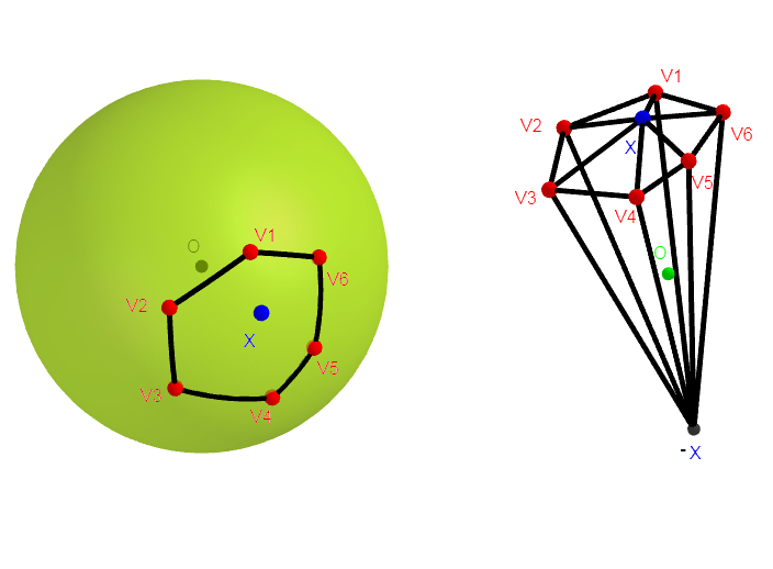
Figure 1: The spherical polygon $P$ and the polyhedron $Q$

Now we state the following theorem

Theorem 1.

Spherical barycentric coordinates, for points inside the polygon P, are given by

$$\psi_{i}(x)=\frac{\phi_{i}(0)}{\phi_{n+2}(0)-\phi_{n+1}(0)}.$$ (2.1)

and on the boundary, by $\psi_{i}(v_{j})=\delta_{ij}$ and

$$\left\{\begin{array}[]{lll}\psi_{j}(x)=\dfrac{\phi_{j}(0)}{\phi_{n+2}(0)}&\mbox{ }\\ \psi_{j+1}(x)=\dfrac{\phi_{j+1}(0)}{\phi_{n+2}(0)}&\mbox{}\\ \psi_{k}(x)=0&\mbox{for}&k\neq j,j+1\end{array}\right.$$ (2.2)

where $\phi_{i},\;i=1,...,n+2$  are any well known 3D barycentric coordinates defined on $Q$
Furthermore, the $\psi_{i}^{\prime}s$ are linear on the edges of $P$.

Proof.

1. The origine $0$ lies in the interior of $Q$ ($0\in[x,-x]$) and it can be written as a linear combination of the vertices $v_{1},v_{2},...,v_{n},x,-x$ as follows

   $$\sum_{i=1}^{n}\phi_{i}(0)\;v_{i}+\phi_{n+1}(0)\;x+\phi_{n+2}(0)\;(-x)=0$$ (2.3)

   Hence

   $$\sum_{i=1}^{n}\phi_{i}(0)\;v_{i}=(\phi_{n+2}(0)-\phi_{n+1}(0))\;x.$$ (2.4)

   The point $p=\sum_{i=1}^{n}\phi_{i}(0)\;v_{i}$ on the left-hand side of  (2.4) belongs to the polyhedral cone $P^{\prime}$ of the vertices $v_{i},i=1,...,n$. This implies that  $\phi_{n+2}(0)-\phi_{n+1}(0)\geq 0$, since the point $q=(\phi_{n+2}(0)-\phi_{n+1}(0))\;x$ on the right-hand side would otherwise be outside of $P^{\prime}$. We claim that $\phi_{n+2}(0)-\phi_{n+1}(0)\neq 0$. On the contrary, suppose that  $\phi_{n+2}(0)-\phi_{n+1}(0)=0$. Then we would have

   $$p=\sum_{i=1}^{n}\phi_{i}(0)\;v_{i}=0$$

   and therefore $\phi_{i}(0)=0,i=1,...,n$. Indeed, suppose there is a $k\in\left\{1,...,n\right\}$ such that $\phi_{k}(0)\neq 0$, then we would have  $-v_{k}=\sum_{i=1,i\neq k}^{n}\dfrac{\phi_{i}(0)}{\phi_{k}(0)}\;v_{i}$, but the point $q=\sum_{i=1,i\neq k}^{n}\dfrac{\phi_{i}(0)}{\phi_{k}(0)}\;v_{i}$ lies in the polyhedral cone $P^{\prime\prime}$ of the vertices $v_{1},,...,v_{k-1},v_{k+1},...,v_{n}$, while $-v_{k}$ is outside of $P^{\prime\prime}$. A contradiction. Now we conclude from the partition of unity property that  $\phi_{n+2}(0)=\phi_{n+1}(0)=\dfrac{1}{2}$. The restriction on facets of the boundary proprety (e) shows that this is only possible if the edge $[x,-x]$  coincides with an edge of $Q$, but this would imply that $x$ coincides with a certain vertex $v_{k}$ of $Q$ and therefore we would have $0=\phi_{k}(0)=\phi_{n+1}(0)=\dfrac{1}{2}$. A contradiction.
   Since x is in the interior of P, equation (2.4) gives

   $$x=\sum_{i=1}^{n}\frac{\phi_{i}(0)}{\phi_{n+2}(0)-\phi_{n+1}(0)}\;v_{i}$$

   From $\phi_{i}(0)\geqslant 0$ and  $\phi_{n+2}(0)-\phi_{n+1}(0)>0$ we conclude that $\psi_{i}(x)\geqslant 0.$ We now compute these coordinates on the boundary using properties (d) and (e), and show that they are linear on each edge and satisfy Lagrange property.

2. On the edges
   If a point $x$ inside $P$ approaches the arc $e_{j}$, then $0$ approaches the interior of the face (triangle) $[-x,v_{j},v_{j+1}]$ of $Q$. The restriction on facets of the boundary proprety (e) shows that in the limit

   $$\phi_{i}(0)\;=0,\;\>for\;i\neq j,j+1,n+2$$ (2.5)

   and therefore $\psi_{i}(x)=\dfrac{\phi_{i}(0)}{\phi_{n+2}(0)}$ for $i=j,j+1$ $\quad(\phi_{n+1}(0)=0\;see\ equation~{}\eqref{moneq6})$
   where $\phi_{i}(0),\;i=1,...,n+2$ are the continuous extensions to the boundary of the 3D barycentric coordinates used in equation (2.1). Therefore, equation equation (2.1) becomes

   $$x = \dfrac{\phi_{j}(0)}{\phi_{n+2}(0)}\;v_{j}+\dfrac{\phi_{j+1}(0)}{\phi_{n+2}(0)}\;v_{j+1}$$ (2.6)

   $$= \psi_{j}(x)\;v_{j}+\psi_{j+1}(x)\;v_{j+1}$$ (2.7)

   where $\psi_{j}(x)=\dfrac{\phi_{j}(0)}{\phi_{n+2}(0)}$ and $\psi_{j+1}(x)=\dfrac{\phi_{j+1}(0)}{\phi_{n+2}(0)}$.
   Spherical barycentric coordinates on the edge $e_{j}$ are therefore given by

   $$\left\{\begin{array}[]{lll}\psi_{j}(x)=\dfrac{\phi_{j}(0)}{\phi_{n+2}(0)}&\mbox{ }\\ \psi_{j+1}(x)=\dfrac{\phi_{j+1}(0)}{\phi_{n+2}(0)}&\mbox{}\\ \psi_{k}(x)=0&\mbox{for}&k\neq j,j+1\end{array}\right.$$

3. Lagrange property
   Equation $(2.7)$ yields

   $$\lim_{x\rightarrow v_{i}}\;x=\displaystyle\lim_{x\rightarrow v_{i}}\;\psi_{i}(x)\;v_{i}+\psi_{i+1}(x)\;v_{i+1}$$

   hence

   $$v_{i}=\displaystyle\lim_{x\rightarrow v_{i}}\;\psi_{i}(x)\;v_{i}+\displaystyle\lim_{x\rightarrow v_{i}}\;\psi_{i+1}(x)\;v_{i+1}$$

   i.e.

   $$\left(1-\displaystyle\lim_{x\rightarrow v_{i}}\;\psi_{i}(x)\right)\;v_{i}=\displaystyle\lim_{x\rightarrow v_{i}}\;\psi_{i+1}(x)\;v_{i+1}$$

   but this means that $v_{i}$ and $v_{i+1}$ are collinear. A contradiction.
   So we must have  $1-\displaystyle\lim_{x\rightarrow v_{i}}\;\psi_{i}(x)=0$  and  $\displaystyle\lim_{x\rightarrow v_{i}}\;\psi_{i+1}(x)=0.$
   Finally, the fact that   $\psi_{j}(x)=0$  for  $j\neq i,i+1$, (see equation (2.4)) completes the proof.

4. Linearity on the edges
   We have $\forall x\in[v_{j},v_{j+1}],\;x=\psi_{j}(x)\;v_{j}+\psi_{j+1}(x)\;v_{j+1}$. To prove the linearity on the edges, it suffices to verify that

   $$\psi_{i}\left[\psi_{j}(x)\;v_{j}+\psi_{j+1}(x)\;v_{j+1}\right]=\psi_{j}(x)\psi_{i}(v_{j})+\psi_{j}(x)\psi_{i}(v_{j+1})$$

   indeed

   • for $i\neq j,j+1$,  we have $\psi_{i}(x)=0$,  hence

     $$\psi_{j}(x)\psi_{i}(v_{j})+\psi_{j}(x)\psi_{i}(v_{j+1}) =\psi_{j}(x)\times 0+\psi_{j}(x)\times 0\qquad(Lagrange\;property\textbf{(d)})$$

     $$=0$$

     $$=\psi_{i}(x)$$

     $$=\psi_{i}\left[\psi_{j}(x)\;v_{j}+\psi_{j+1}(x)\;v_{j+1}\right]\quad(x=\psi_{j}(x)\;v_{j}+\psi_{j+1}(x)\;v_{j+1})$$

   • for $i=j$

     $$\psi_{j}(x)\psi_{i}(v_{j})+\psi_{j}(x)\psi_{i}(v_{j+1}) =\psi_{j}(x)\psi_{j}(v_{j})+\psi_{j}(x)\psi_{j}(v_{j+1})\qquad(i=j)$$

     $$=\psi_{j}(x)\times 1+\psi_{j}(x)\times 0\qquad(Lagrange\;property\textbf{(d)})$$

     $$=\psi_{j}(x)$$

     $$=\psi_{i}(x)\qquad(i=j)$$

     $$=\psi_{i}\left[\psi_{j}(x)\;v_{j}+\psi_{j+1}(x)\;v_{j+1}\right]\quad(x=\psi_{j}(x)\;v_{j}+\psi_{j+1}(x)\;v_{j+1})$$

   • same for $i=j+1.$

∎

Remark 1.

The new coordinates are more general than the classical ones in the sens that:

1. Unlike in the classical approach, they are well defined inside $P$ without need of any continuous extension to the special case where the angle $\theta_{i}$ between $x$ and any vertex of $P$ is half of pi (i.e $\langle x,v_{i}\rangle=0$)

2. The classical approach works only in the case where $\langle x,v_{i}\rangle>0$ for all i, while our approach works perfectly regardless of the signs of the $\langle x,v_{i}\rangle$

3. In the limit case where all vertices $v_{i}$ lying on a great circle $C$, our approach computes spherical barycentric coordinates of any point $x$ on the sphere not lying on $C$

2.1 Comparison between new and existing coordinates

We adopt the following notation:
NC: The new coordinates introduced above
CC: Spherical coordinates introduced by Langer et al [10]
CF: Spherical coordinates introduced by Floater [6]
MV: Mean value coordinates
WC: Wachspress coordinates

2.1.1 Mean value coordinates

We show that NC and CC mean value coordinates coincide in the case where $\langle x,v_{i}\rangle>0$ for all i.

• 3D mean value coordinates of [4] are given, for a point x inside the kernel of a given polyhedron, by

  $$\psi_{i}(x)=\dfrac{w_{i}(x)}{w}\quad\quad\quad\omega_{i}=\dfrac{1}{\parallel v_{i}-x\parallel}\;\sum_{T\in T(v_{i})}\;\;\mu_{i,T}$$ (2.8)

  where $\mu_{i,T}=\dfrac{\beta_{jk}+\beta_{ij}\;\langle n_{ij},n_{jk}\rangle+\beta_{ki}\;\langle n_{ki},n_{jk}\rangle}{\langle 2e_{i},n_{jk}\rangle}$ and $\beta_{rs}$ is the angle between the two line segments $[x,v_{r}]$ and $[x,v_{s}]$, $n_{rs}=\dfrac{e_{r}\times e_{s}}{\parallel e_{r}\times e_{s}\parallel}$, $e_{i}=\dfrac{v_{i}-x}{\parallel v_{i}-x\parallel}$ and $T(v_{i})$ denotes the set of faces (triangles) $T$ incident to the vertex $v_{i}$.
  Now, we consider the two faces $T1=[v_{i},v_{i+1},x]$ and $T2=[v_{i},-x,v_{i+1}]$ and compute $\mu_{i,T1}$ and $\mu_{i,T2}$.
  

  $$\mu_{i,T1}=\dfrac{\beta_{(i+1)(n+1)}+\beta_{i(i+1)}\left\langle\dfrac{v_{i}\times v_{i+1}}{\parallel v_{i}\times v_{i+1}\parallel},\dfrac{v_{i+1}\times x}{\parallel v_{i+1}\times x\parallel}\right\rangle+\beta_{(n+1)i}\left\langle\dfrac{x\times v_{i}}{\parallel x\times v_{i}\parallel},\dfrac{v_{i+1}\times x}{\parallel v_{i+1}\times x\parallel}\right\rangle}{\left\langle 2v_{i},\dfrac{v_{i+1}\times x}{\parallel v_{i+1}\times x\parallel}\right\rangle}$$

  and

  $$\mu_{i,T2}=\dfrac{\beta_{(n+2)(i+1)}+\beta_{i(n+1)}\left\langle\dfrac{v_{i}\times-x}{\parallel v_{i}\times-x\parallel},\dfrac{-x\times v_{i+1}}{\parallel-x\times v_{i+1}\parallel}\right\rangle+\beta_{(i+1)i}\left\langle\dfrac{v_{i+1}\times v_{i}}{\parallel v_{i+1}\times v_{i}\parallel},\dfrac{-x\times v_{i+1}}{\parallel-x\times v_{i+1}\parallel}\right\rangle}{\left\langle 2v_{i},\dfrac{-x\times v_{i+1}}{\parallel-x\times v_{i+1}\parallel}\right\rangle}$$

  hence

  $$\mu_{i,T1}=\dfrac{\theta_{i+1}+\beta_{i(i+1)}\left\langle\dfrac{v_{i}\times v_{i+1}}{\parallel v_{i}\times v_{i+1}\parallel},\dfrac{v_{i+1}\times x}{\parallel v_{i+1}\times x\parallel}\right\rangle-\theta_{i}\cos\alpha_{i}}{\left\langle 2v_{i},\dfrac{v_{i+1}\times x}{\parallel v_{i+1}\times x\parallel}\right\rangle}$$

  and

  $$\mu_{i,T2}=\dfrac{\pi-\theta_{i+1}-(\pi-\theta_{i})\cos\alpha_{i}-\beta_{i(i+1)}\left\langle\dfrac{v_{i}\times v_{i+1}}{\parallel v_{i}\times v_{i+1}\parallel},\dfrac{v_{i+1}\times x}{\parallel v_{i+1}\times x\parallel}\right\rangle}{\left\langle 2v_{i},\dfrac{v_{i+1}\times x}{\parallel v_{i+1}\times x\parallel}\right\rangle}$$

  where $\theta_{i}=\widehat{(x,v_{i})}$ and $\alpha_{i}=\widehat{(x\times v_{i},x\times v_{i+1})}$. Hence

  $$\mu_{i,T1}+\mu_{i,T2}=\dfrac{\pi(1-\cos\alpha_{i})}{\dfrac{\langle 2v_{i},v_{i+1}\times x\rangle}{\sin\theta_{i}}}$$ (2.9)

  The term ${V=\langle v_{i},v_{i+1}\times x\rangle}$ in the denominator of equation (2.9) is the volume of the parallelepiped determined by the vectors $v_{i},v_{i+1}$ and $x$ and it is given by the formula

  $$V=\sqrt{1+2\cos\theta_{i}\cos\widehat{(v_{i},v_{i+1})}\cos\theta_{i+1}-{\cos^{2}\theta_{i}}-{\cos^{2}\widehat{(v_{i},v_{i+1})}}-{\cos^{2}\theta_{i+1}}}$$ (2.10)

  using the identity relating the cross product to the scalar triple product

  $$\langle a\times b,c\times d\rangle=\langle a,c\rangle\langle b,d\rangle-\langle a,d\rangle\langle b,c\rangle$$ (2.11)

  we obtain

  $$\langle v_{i}\times x,v_{i+1}\times x\rangle=\langle v_{i},v_{i+1}\rangle-\langle v_{i},x\rangle\langle v_{i+1},x\rangle$$

  i.e.

  $$\parallel v_{i}\times x\parallel\parallel v_{i+1}\times x\parallel\cos\alpha_{i}=\cos\widehat{(v_{i},v_{i+1})}-\cos\theta_{i}\cos\theta_{i+1}$$

  therefore

  $$\sin\theta_{i}\sin\theta_{i+1}\cos\alpha_{i}=\cos\widehat{(v_{i},v_{i+1})}-\cos\theta_{i}\cos\theta_{i+1}$$

  and so

  $$\cos\widehat{(v_{i},v_{i+1})}=\sin\theta_{i}\sin\theta_{i+1}\cos\alpha_{i}+\cos\theta_{i}\cos\theta_{i+1}$$ (2.12)

  By inserting this term into equation (2.10) and after a simple calculation we find

  $$V=\sin\theta_{i}\sin\theta_{i+1}\sin\alpha_{i}$$

  Now, we have

  $$\mu_{i,T1}+\mu_{i,T2}=\dfrac{\pi\;{\sin^{2}\dfrac{\alpha_{i}}{2}}}{\dfrac{\sin\theta_{i}\sin\theta_{i+1}2\sin\dfrac{\alpha_{i}}{2}\cos\dfrac{\alpha_{i}}{2}}{\sin\theta_{i+1}}}$$

  i.e.

  $$\mu_{i,T1}+\mu_{i,T2}=\dfrac{\pi\;{\tan\dfrac{\alpha_{i}}{2}}}{2\sin\theta_{i}}$$

  
  

  we do the same for the faces $T3=[v_{i},x,v_{i-1}]$ and $T4=[v_{i},v_{i-1},-x]$ and we find

  $$\mu_{i,T3}+\mu_{i,T4}=\dfrac{\pi\;\tan\dfrac{\alpha_{i-1}}{2}}{2\sin\theta_{i}}$$

  Now, the weight of the origin $0$ with respect to the vertex $v_{i}$ is given by

  $$\omega_{i}=\mu_{i,T1}+\mu_{i,T2}+\mu_{i,T3}+\mu_{i,T4}=\dfrac{\pi\;(\tan\dfrac{\alpha_{i}}{2}+\tan\dfrac{\alpha_{i-1}}{2})}{2\sin\theta_{i}}$$

  we need to compute the weights of the vertices $x$ and $-x$. In the same way we get

  $$\mu_{n+2,T2}-\mu_{n+1,T1}=\dfrac{\pi\left\langle\dfrac{v_{i+1}\times x}{\parallel v_{i+1}\times x\parallel},\dfrac{v_{i}\times v_{i+1}}{\parallel v_{i}\times v_{i+1}\parallel}\right\rangle+\pi\left\langle\dfrac{x\times v_{i}}{\parallel x\times v_{i}\parallel},\dfrac{v_{i}\times v_{i+1}}{\parallel v_{i}\times v_{i+1}\parallel}\right\rangle}{\left\langle 2v_{i},\dfrac{v_{i+1}\times x}{\parallel v_{i}\times v_{i+1}\parallel}\right\rangle}$$

  i.e.

  $$\mu_{n+2,T2}-\mu_{n+1,T1}=\dfrac{\pi\left\langle\dfrac{v_{i+1}\times x}{\parallel v_{i+1}\times x\parallel},v_{i}\times v_{i+1}\right\rangle+\pi\left\langle\dfrac{x\times v_{i}}{\parallel x\times v_{i}\parallel},v_{i}\times v_{i+1}\right\rangle}{\left\langle 2v_{i},v_{i}\times v_{i+1}\right\rangle}.$$

  By using equations  (2.11) and  (2.12), we find

  $$\left\langle\dfrac{v_{i+1}\times x}{\parallel v_{i+1}\times x\parallel},v_{i}\times v_{i+1}\right\rangle = \dfrac{\cos\theta_{i+1}\cos\widehat{(v_{i},v_{i+1})}-\cos\theta_{i}}{\sin\theta_{i+1}}$$

  $$= \dfrac{\cos\theta_{i+1}\sin\theta_{i}\sin\theta_{i+1}\cos\alpha_{i}-\cos\theta_{i}\cos^{2}\theta_{i+1}}{\sin\theta_{i+1}}$$

  $$= \dfrac{\cos\theta_{i+1}\sin\theta_{i}\sin\theta_{i+1}\cos\alpha_{i}-\cos\theta_{i}\sin^{2}\theta_{i+1}}{\sin\theta_{i+1}}$$

  $$= \cos\theta_{i+1}\sin\theta_{i}\cos\alpha_{i}-\cos\theta_{i}\sin\theta_{i+1}$$

  and

  $$\left\langle\dfrac{x\times v_{i}}{\parallel x\times v_{i}\parallel},v_{i}\times v_{i+1}\right\rangle=\cos\theta_{i}\sin\theta_{i+1}\cos\alpha_{i}-\cos\theta_{i+1}\sin\theta_{i}$$

  hence

  $$\mu_{n+2,T2}-\mu_{n+1,T1}=\dfrac{\pi\cot\theta_{i+1}-\pi\cot\theta_{i+1}\cos\alpha_{i}+\pi\cot\theta_{i}-\pi\cot\theta_{i}\cos\alpha_{i}}{2\sin\alpha_{i}}$$

  And then

  $$\mu_{n+2,T2}-\mu_{n+1,T1} = \dfrac{\pi(\cot\theta_{i+1}+\cot\theta_{i})(1-\cos\alpha_{i})}{2\sin\alpha_{i}}$$

  $$= \dfrac{\pi}{2}(\cot\theta_{i+1}+\cot\theta_{i})\tan\dfrac{\alpha_{i}}{2}$$

  now

  $$w_{n+2}-w_{n+1} = \sum_{i=1}^{n}\mu_{n+2,T2}-\mu_{n+1,T1}$$

  $$= \sum_{i=1}^{n}\dfrac{\pi}{2}(\cot\theta_{i+1}+\cot\theta_{i})\tan\dfrac{\alpha_{i}}{2}$$

  $$= \dfrac{\pi}{2}\left(\sum_{i=1}^{n}\cot\theta_{i}\tan\dfrac{\alpha_{i}}{2}+\sum_{i=1}^{n}\cot\theta_{i+1}\tan\dfrac{\alpha_{i}}{2}\right)$$

  by setting $k=i+1$ and use the fact that $v_{i+n}=v_{i}$, we get

  $$w_{n+2}-w_{n+1} = \dfrac{\pi}{2}\left(\sum_{i=1}^{n}\cot\theta_{i}\tan\dfrac{\alpha_{i}}{2}+\sum_{k=2}^{n+1}\cot\theta_{k}\tan\dfrac{\alpha_{k-1}}{2}\right)$$

  $$= \dfrac{\pi}{2}\sum_{i=1}^{n}\cot\theta_{i}\left(\tan\dfrac{\alpha_{i}}{2}+\tan\dfrac{\alpha_{i-1}}{2}\right)$$

  The new coordinates $\psi_{i}(x)$ are therefore given in terms of the classical coordinates $\lambda_{i}(x)$ by

  $$\psi(x)=\frac{\phi_{i}(0)}{\phi_{n+2}(0)-\phi_{n+1}(0)}=\dfrac{w_{i}}{w_{n+2}-w_{n+1}} = \dfrac{\dfrac{\pi\;\left(\tan\dfrac{\alpha_{i}}{2}+\tan\dfrac{\alpha_{i-1}}{2}\right)}{2\sin\theta_{i}}}{\dfrac{\pi}{2}\sum_{i=1}^{n}\cot\theta_{i}\left(\tan\dfrac{\alpha_{i}}{2}+\tan\dfrac{\alpha_{i-1}}{2}\right)}$$

  $$= \lambda_{i}(x)$$

• figure  2 provides a visual example which confirms that both coordinates coincide.

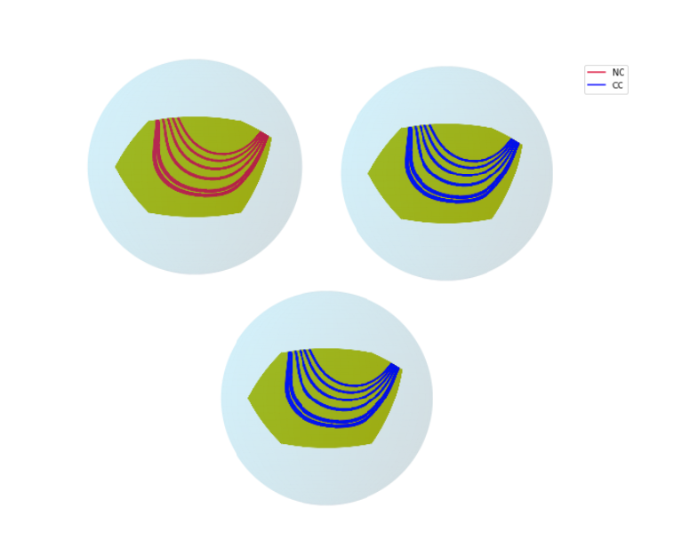
Figure 2: Contour lines of the MV with respect to the vertex $v_{1}$ for values of $\psi_{1}$ in $[0.09,0.10]$, $[0.11,0.12]$, $[0.17,0.18]$, $[0.23,0.24]$, $[0.30,0.29]$ and $[0.35,0.36]$

2.1.2 Wachspress coordinates

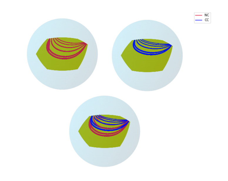
Figure 3: Contour lines of the WC with respect to the vertex $v_{1}$ for values of $\psi_{1}$ in $[0.09,0.10]$, $[0.11,0.12]$, $[0.17,0.18]$, $[0.23,0.24]$, $[0.30,0.29]$ and $[0.35,0.36]$

Figure  3 (respectively  4), provides contour lines of WC for NC and CC (respectively NC and CF). The coordinates seem to differ: we intend to give the proof of the general case in the future.

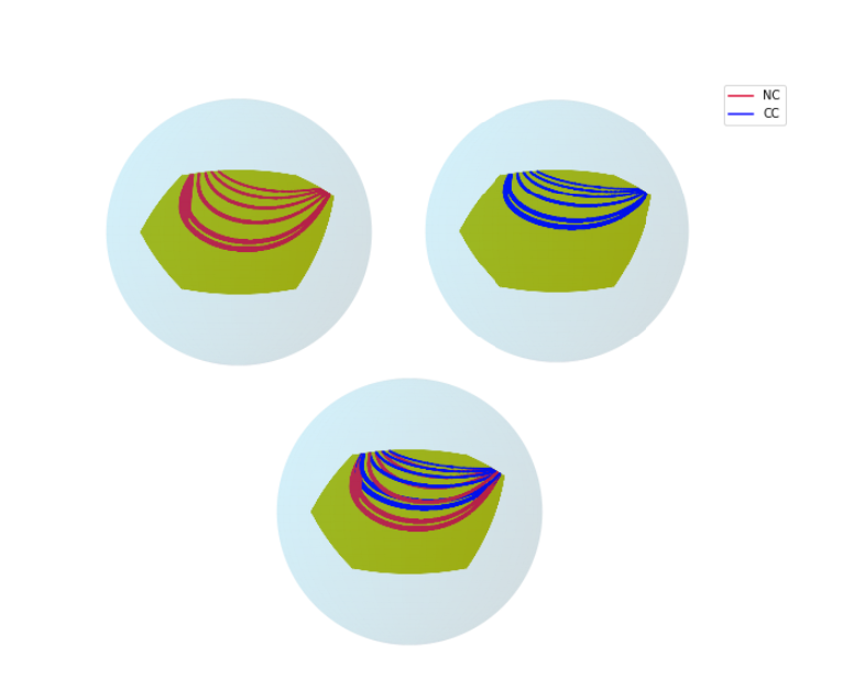
Figure 4: Contour lines of the WCF with respect to the vertex $v_{1}$ for values of $\psi_{1}$ in $[0.09,0.10]$, $[0.11,0.12]$, $[0.17,0.18]$, $[0.23,0.24]$, $[0.30,0.29]$ and $[0.35,0.36]$

3 Conclusion

The new approach gives us a direct relationship between spherical barycentric coordinates and 3D barycentric coordinates via the origin $0$. Their resulting coordinates are more general than the classical ones.

References

• [1] P. Alfred, M. Neamtu, L. L. Schumaker: Bernstein-BΓ©zier polynomials on spheres and sphere-like surfaces Comput. Aided Geom. Des. 13, 4 (1996), 333–349.
• [2] M. Arroyo, M. Ortiz: Local maximum-entropy approximation schemes: a seamless bridge between finite elements and meshfree methods Int. J. Numer. Meth. Engng 65, 13 (2006), 2167–2202.
• [3] M. Desbrun, M. Meyer, P. Alliez: Intrinsic parameterizations of surface meshes Computer Graphics Forum 21 (2002), 209–218.
• [4] M. S. Floate, G Kos, M. Reimers: Mean value coordinates in 3D Comp.Aided.Geom.design 22(2005),623 631
• [5] M. S. Floater: Mean value coordinates Computer Aided Geometric Design 20, 1 (2003), 19–27. 1, 2, 5, 6
• [6] M. S. Floater: Generalized barycentric coordinates and applications Acta Numerica (2016), pp. 001– doi:10.1017/S09624929c
• [7] H. Gouraud: Continuous shading of curved surfaces IEEE Trans. Computers C-20, 6 (1971), 623–629.
• [8] K. Hormann, N. Sukumar: Generalized Barycentric Coordinates in Computer Graphics and Computational Mechanics Taylor and Francis, CRC Press, 2017.
• [9] T. Ju, P. Liepa, and J. Warren: A general geometric construction of coordinates in a convex simplicial polytope Computer Aided Geometric Design, 24(3):161–178, 2007.
• [10] T. Langer, A. Balayev, H P. Seidel: Spherical Barycentric Coordinates Eurographics Symposium on Geometry Processing (2006) Konrad Polthier, Alla Sheffer (Editors).
• [11] A F. Mobius: Β Der barycentrische Calcul.. Johann Ambrosius Barth, Leipzig, 1827.
• [12] U. Pinkall and K. Polthier: Computing discrete minimal surfaces and their conjugates Experimental Mathematics, 2(1):15–36, 1993.
• [13] B. T. Phong: Illumination for computer generated pictures Communications of ACM 18, 6 (1975), 311–317.
• [14] J. Schreiner, A. Asirvatham, E. Praun, H. Hoppe: Inter-surface mapping ACM Trans. Graph. 23, 3(2004), 870–877.
• [15] T. W. Sederberg, S. R. Parry: Freeform deformation of solid geometric models In Computer Graphics, Proceedings of ACM SIGGRAPH (1986), pp. 151–160.
• [16] R. Sibson: A vector identity for the Dirichlet tessellation Math. Proc. Cambridge Phil. Soc. 87 (1980).
• [17] J. Tao, S. Schaefer, J. Warren, M. Desbrun: A geometric construction of coordinates for convex polyhedra using polar duals In Proceedings of the Symposium on Geometry Processing (2005), pp. 181–186.
• [18] Tao Ju, Scott Schaefer, and Joe Warren: Mean value coordinates for closed triangular meshes In ACM SIGGRAPH 2005 Papers. ACM, 561–566
• [19] A Rational Finite Element Basis E. L Wachspress: A Rational Finite Element Ba- vol. 114. Academic Press, New York, 1975.
• [20] Joe Warren, Scott Schaefer, Anil N Hirani, and Mathieu Desbrun: Barycentric coordinates for convex sets Advances in computational mathematics 27, 3 (2007), 319–338