Using the Projected Belief Network at High Dimensions

Abstract

The projected belief network (PBN) is a layered generative network (LGN) with tractable likelihood function, and is based on a feed-forward neural network (FFNN). There are two versions of the PBN: stochastic and deterministic (D-PBN), and each has theoretical advantages over other LGNs. However, implementation of the PBN requires an iterative algorithm that includes the inversion of a symmetric matrix of size $M\times M$ in each layer, where $M$ is the layer output dimension. This, and the fact that the network must be always dimension-reducing in each layer, can limit the types of problems where the PBN can be applied. In this paper, we describe techniques to avoid or mitigate these restrictions and use the PBN effectively at high dimension. We apply the discriminatively aligned PBN (PBN-DA) to classifying and auto-encoding high-dimensional spectrograms of acoustic events. We also present the discriminatively aligned D-PBN for the first time.

I Introduction

I-A Motivation: Advantages of PBN

The projected belief network (PBN) is a layered generative network (LGN) with tractable likelihood function, and is based on a feed-forward neural network (FFNN). There are two versions of the PBN: stochastic and deterministic, and each has theoretical advantages over other layered generative networks.

It has recently been shown that the information at the output of a dimension-reducing transformation can be maximized using probability density function projection (PDF projection) [1]. PDF projection estimates the distribution of the input data, simultaneously with a dimension-reducing transformation that extracts the latent variables [2, 3]. The method is more general than other methods of non-linear dimension reduction (NLDR) [4, 5, 6, 7, 8]. Implementing PDF projection in a neural network architecture is called projected belief network (PBN) [9, 10, 11, 12]. As a result, the PBN is the most direct and general way to apply NLDR in a neural network architecture.

The LF of other widely used LGNs can only be obtained by intractable integration (marginalizing) over the hidden variables. They must rely on a surrogate cost function in order to approximate LF training. Examples are contrastive divergence (CD) to train restricted Boltzmann machines [13, 14], and Kullback Leibler divergence to train variational auto-encoder (VAE) [15], or an adversarial discriminative network to train generative adversarial networks (GAN) [16]. On the other hand, since the PBN generates data by manifold sampling, it posesses a tractable likelihood function (LF) that allows direct gradient-based training.

The deterministic PBN (D-PBN) can be used as an auto-encoder [11, 9] and has theoretical advantage over conventional auto-encoders. While other auto-encoders use an empirical reconstruction network, the deterministic PBN reconstructs input data by backing up (back-projecting) through the same feed-forward neural network (FFNN) that was used to extract the features. In each layer, it selects the conditional mean estimate of the layer input based on a maximum entropy prior, a type of optimal estimator.

Another advantage of the PBN and D-PBN is that they are based on a FFNN. Therefore, a single FFNN can be simultaneously a generative and a discriminative network [12]. This offers the most direct way to combine the advantages of both network types. A number of variations of this concept have been proposed. The PBN or D-PBN cost functions can be used as a regularization for discriminative neural networks [12], or the opposite: discriminative cost function can be used to “align” a PBN to decision boundaries to create better-performing generative models [17]. We will use this approach in this paper to test the PBN and D-PBN at high dimensions.

I-B Discriminative Alignment of PBN

It was shown in [17] that a generative classifier (a PBN) can compete with state of the art discriminative classifiers. This seems to contradict the widely-held belief that the generative task is much harder, and unnecessary for classifying [18]. However, generative models are useful in their own right, and can be applied in some tasks where discriminative classifiers cannot [19]. A generative classifier than can perform as well as a discriminative classifier, is highly desireable.

Sand box analogy. Discriminative alignment can be understood in terms of the conceptual image of a sand box enclosed by a wooden frame. The frame can be thought of as the discriminative task, separating the probability mass (the sand) from the other classes at the decision boundaries. The generative model can be thought of as heaping the sand at the places where data is more likely. The two tasks can be achieved simultaneously using discriminative alignment of a PBN.

Despite the benefits it offers, the PBN is bound by restrictions that also affect the discriminative model that it may share : (a) dimension-reducing layers, (b) no max-pooling in convolutional layers, (c) no dropout regularization, and (d) no batch normalization. On the positive side, L2 regularization can be used, and the generative cost function can be seen as a form of regularization in itself [12], and one can avoid the restriction on dimension-reducing layers using the method in Section III-E.

I-C Computational Challenge of PBN

Despite these theoretical advantages, implementation of the PBN requires in each layer the inversion of a $M\times M$ symmetric matrix where $M$ is the layer output dimension. In convolutional layers, $M$ can be extremely large because it is the product of the number of kernels with the size of the feature maps. Depending on the type of PBN layer (i.e depending in the type of maximum entropy prior distribution), this matrix may need to be inverted for each sample in a mini-batch.

I-D Paper Organization and Contributions

We begin by a mathematical review of PBN and D-PBN in Section II, explaining the computational challenge of PBN at high dimensions, then suggest new approaches to applying PBN at high dimensions in Section III. Experimental results are provided in Section IV including a novel variation of PBN, called D-PBN-DA in Section IV-H.

II The PBN: Review

II-A PDF Projection

A PBN is just a layer-wise application of PDF projection. In probability density function (PDF) projection, one defines an $N\times 1$ input vector ${\bf x}$, and a transformation ${\bf z}=T({\bf x})$ producing the $M\times 1$ output vector ${\bf z}$, where $M<N$. Suppose we have data ${\bf x}$ drawn from some distribution $p({\bf x})$ with support on $\mathbb{X}\subseteq\mathbb{R}^{N}$, that we’d like to estimate. Although $p({\bf x})$ is unknown, we know $g({\bf z})$, which is an estimate of the feature distribution of ${\bf z}$, where ${\bf x}$ is drawn from $p({\bf x})$ and ${\bf z}=T({\bf x})$, and has support on $\mathbb{Z}\subseteq\mathbb{R}^{M}$. To estimate $p({\bf x})$ based on knowing $g({\bf z})$, we first define a reference (or prior) distribution $p_{0}({\bf x})$ for which we know $p_{0}({\bf z})$, the mapping of $p_{0}({\bf x})$ through $T({\bf x})$. Then, the PDF projection theorem [2] states that the function

$$G({\bf x};T,p_{0},g)=\frac{p_{0}({\bf x})}{p_{0}({\bf z})}\;g({\bf z}),$$ (1)

where ${\bf z}=T({\bf x})$, is a PDF on $\mathbb{X}$ (it integrates to 1) and is among the class of PDFs which map to distribution $g({\bf z})$ through $T({\bf x})$. Simply stated, $G({\bf x};T,p_{0},g)$ is an estimate of $p({\bf x})$ based on prior distribution $p_{0}({\bf x})$ and feature PDF estimate $g({\bf z})$.

The biggest challenge on PDF projection is the derivation of $p_{0}({\bf z})$. When $p_{0}({\bf x})$ is a canonical reference distribution, the feature distribution $p_{0}({\bf z})$ is known in closed form for many types of transformations [20]. For an even broader class of reference distributions and transformations, $p_{0}({\bf z})$ is not known, but the moment generating function (MGF) is known exactly. In these cases, we can invert the MGF using the saddle point approximation (see eq. (16) in [20]). We note that the term “approximation” is misleading because the error can be neglected for all practical purposes [17].

II-B The PBN

For complex transformations, such as a neural network, $p_{0}({\bf z})$ may be difficult or impossible to derive, so we apply PDF projection recursively (layer-wise). This results in a projected belief network (PBN) [21], where the likelihood function (LF) $G({\bf x};T,p_{0},g)$ becomes a product of terms, each term being the application of (1) to a layer (see eq. (1) in [12]).

II-C Finding the Saddle Point

Each term in the LF of a PBN requires computing the saddle point. Let ${\bf x}\subseteq\mathbb{R}^{N}$ be the input of a layer, where $N$ is the dimension. Let ${\bf z}\subseteq\mathbb{R}^{M}$ be the output of the linear transformation given by ${\bf z}={\bf W}^{\prime}{\bf x}$. This is the dimension-reducing linear transformation used in each layer of a neural network before application of the activation function. Note that this equation holds both for dense (fully connected) and convolutional layers. Although convolutional layers are implemented by efficient convolution, there exists at least theoretically an $N\times M$ matrix ${\bf W}$.

The saddle point $\hat{{\bf h}}$ is the $M\times 1$ vector ${\bf h}$ that solves

$${\bf W}^{\prime}\lambda\left(\mbox{\boldmath$\alpha$}_{0}+{\bf W}{\bf h}\right)={\bf z},$$ (2)

where $N\times 1$ constant vector $\mbox{\boldmath$\alpha$}_{0}$ and element-wise activation function $\lambda(\;)$ depend on the chosen MaxEnt prior [9].

Equation (2) is solved by an iterative algorithm (Newton-Raphson) that involves inverting the matrix ${\bf C}(\hat{{\bf h}})={\bf W}^{\prime}\Lambda{\bf W}$, where $\Lambda$ is the $N\times N$ diagonal matrix with diagonal $\lambda^{\prime}(\alpha_{1}),\lambda^{\prime}(\alpha_{2}),\ldots\lambda^{\prime}(\alpha_{N})$, where $\lambda^{\prime}(\alpha)$ is the value of the first derivative of $\lambda\left(\alpha\right)$ with repect to $\alpha$, and $\mbox{\boldmath$\alpha$}=\mbox{\boldmath$\alpha$}_{0}+{\bf W}\hat{{\bf h}}$.

II-D Using the Saddle Point

The deterministic PBN (D-PBN) reconstructs ${\bf x}$ from ${\bf z}$ and the saddle point as follows [9]:

$$\hat{{\bf x}}=\lambda\left(\mbox{\boldmath$\alpha$}_{0}+{\bf W}\hat{{\bf h}}\right)$$ (3)

A multi-layer D-PBN is created by propagating the estimate backward in the network [9, 11]. The stochastic PBN uses the saddle point to compute terms in the LF. Specifically, $p_{0}({\bf z})$ is written using equation (16) in [20], where the saddle point is written $\hat{\mbox{\boldmath$\lambda$}}$ and $p_{0}({\bf z})$ is written $p_{z}({\bf u})$.

III Dimension Mitigation

The computational challenges of using PBN at high dimensions, outlined in Section I-C, can be mitigated using the following approaches.

III-A Seamless Streaming and Reconstruction

Large data samples that have a time dimension, such as audio recordings can be broken into smaller segments and processed by a sliding window. There is an implicit assumption of independence between segments here that can be approximately true if the segments are large enough. As long as the sliding window is wide enough to capture enough temporal information, the generative model can provide meaningful and significant dimension reduction with high information content. The collection of output features, i.e. the “stream” of output features can be used to reconstruct the complete event, and further feature dimension reduction can be done on the assembled stream so that temporal information spanning larger time durations can be extracted downstream.

For seamless reconstruction, the sliding windows must overlap by exactly the right amount, so that the assembled output stream is no different than what would have been created by the same processing on the entire event. Any temporal processing, i.e. temporal convolution, must be done without edge effects. For this reason, convolutions in convolutional network layers must be done without zero-padding.

III-B Gaussian Layers

A very significant speed-up is afforded by Gaussian layers. In a Gaussian layer, the Gaussian MaxEnt prior is assumed, and $\lambda(x)=x$ is the linear activation, meaning that ${\bf C}(\hat{{\bf h}})={\bf C}={\bf W}^{\prime}{\bf W}$ is independent of $\hat{{\bf h}}$ and $\mbox{\boldmath$\alpha$}_{0}={\bf 0}$, so (2) can be solved in closed form, i.e. $\hat{{\bf h}}=({\bf W}^{\prime}{\bf W})^{-1}{\bf z},$ and needs to be done only once per mini-batch. Note that for convolutional layers, all operations are done by convolution, and matrix ${\bf W}$ never needs to be actually created.

Using Gaussian layers, however, assumes that the layer input has support on $\mathbb{R}^{N}$, which means that activation functions should be avoided in the layer that precedes a Gaussian layer to attain a good PDF estimate using PDF projection. Using linear activations in the first few layers, and then non-linear activations in middle and low-dimensional layers may be an effective compromise.

III-C Gaussian Layer Groups (GLG)

For very large hidden variable dimensions, using a Gaussian layer may be prohibitive - even allocating memory for ${\bf C}$ may be difficult. In these cases, it is possible to use several Gaussian layers in a row, ending in a manageable output dimension, then grouping the linear transformations so that they are representable by a single linear transformation with low output dimension $M$, and small ${\bf C}$. After the GLG, non-linear activation functions can be used. As long as $M$ at the group output is large enough, significant functional approximation power is afforded by the network.

III-D Dimension-Preserving Layers

If a layer input and output have the same dimension, it is a dimension-preserving (1:1) transformation layer and computing the saddle point is not required. It is only necessary to solve for the determinant of the Jacobian matrix of the transformation as a whole.

III-E Expand-Contract Groups (ECG)

To afford even greater functional approximation power, it is possible to expand the hidden variable dimension using a series of high-dimensional network layers, then reduce the dimension back down to what it was at the start. This group of layers, seen as a unit, can be analyzed as a dimension-preserving (1:1) transformation, as if it was a single dimension-preserving layer.

III-F Direct Saddle Point Estimation

One can find $\hat{{\bf h}}$, the solution to (2), by direct inversion using a neural network by training on sample pairs ${\bf z}$, $\hat{{\bf h}}$. Error in the result is removed by a few iterations of the Newton-Raphson algorithm.

IV Experimental Results

IV-A Experimental Goal: Discriminative Alignment of PBN

The goal of our first experiment was to show that discriminative alignment, which was demonstrated previously on input data data dimensions of 196 and 900 [17], can be used on a different data set with much higher dimension. Discriminative alignment is explained in Section I-B and further details are given in Section IV-F.

IV-B Data and Feature Extraction

The Office Sounds database [22, 23] contains twenty-four signal classes containing 102 samples of each class, a total of 2448 example sounds. Most of the sounds are created by dropping common objects or operating office tools such as scissors or staplers. All time-series are 16128 samples long (1/2 second in duration at 32000 Hz). We selected six of the twenty-four classes that had the highest inter-class errors. These classes were “skit”, “sciss”, “pret”, “pens”, “paper”, and “jing” and are seen on the top row of Figure 1. There were 102 samples of each class, so 612 samples total. The emphasis is to achieve very high correct classification performance on acoustic data with few training samples. The 612 events were divided into training and testing sets of 306 each. We conducted two-fold hold-out in which we trained on half of the data and tested using the other half, then repeated the experiment with the data switched. To extract features, we segmented each time-series sample into size-384 windows with 2/3 overlap, producing 126 segments per time series. We then took the FFT, magnitude-squared, then the log. The features were therefore $126\times 193$, or dimension 24,318.

IV-C Network, Algorithm, and Hardware

The network consisted of seven layers:

1. Convolutional with 6 ($9\times 10$) kernels, with ($3\times 3$) downsampling, linear activation,

2. Convolutional with 36 ($7\times 8$) kernels, with ($3\times 3$) downsampling, linear activation,

3. Convolutional with 96 ($8\times 7$) kernels, with ($2\times 3$) downsampling, linear activation,

4. Dense with 512 neurons, linear activation.

5. Dense with 256 neurons, TG activation.

6. Dense with 128 neurons, TG activation.

7. Classifier layer, dense with 6 neurons.

The “TG” activation is the truncated Gaussian activation [24], similar in behavior to softplus, not unlike leaky Relu, but continuous. All convolutions used the “valid” border mode, so no zero-padding was used and the output feature maps are smaller than the input map, even without down-sampling. The output feature maps of the five layers have shapes (6, 40, 62), (36, 12, 19), (96, 3, 5), 512, 256, 128, and 6, with total dimensions 14880, 8208, 1440, 512, 256, 128, and 6 respectively.

IV-D Dimension Mitigation and Training

Seamless streaming was not neccessary for this data set because the entire event of dimension 24,318 could be processed. However, note that the first five layers form a GLG with output dimension 256, so the saddle point can be solved by inverting a matrix ${\bf C}$ of only $256\times 256$, just once per mini-batch. Interestingly, the dominant computational load in the network involves the 6-th layer, which requires inverting a $128\times 128$ matrix ${\bf C}(\hat{{\bf h}})$ on each sample of the mini-batch. The algorithm maximized the log-likelihood of the PBN. We used direct saddle point estimation using a symmetric linear transformation, followed by some Newton-Raphson iterations. Surprisingly, a linear transformation $\hat{{\bf h}}={\bf A}^{\prime}{\bf A}{\bf z}$, results in a small residual error. We used a mini-batch size of 306, which was all of the training data. The large batch size made best use of the GPU. On a Quadro P6000 GPU with 32 bit (single precision) we were able compute an epoch in 8.5 seconds, or 11 seconds with 64 bit precision. All experiments were done using the PBN Toolkit, which is a graphical tool using the Theano framework. Each model required about 500 epochs.

IV-E Benchmark Network

For a performance benchmark, we applied conventional deep convolutional neural network (CNN) with state of the art training methods. We used the same network structure as the PBN, but the CNN was not bound by the restrictions of the PBN. Therefore, we used TG activation function in each layer (linear activation was not used), and we used max-pooling in the convolutional layers (not down-sampling), dropout, and L2 regularization.

IV-F PBN and DNN Training

A separate PBN was trained for each class by maximizing a combined generative-discriminative target function consisting of (a) the PBN log-likelihood function, and (b) the negative cross-entropy classifier cost for discriminating the corrsponding class from all other classes. The first component was given a weight of one for all samples from the target class, and zero for all samples from other classes. The second component was weighted by one for all classes. This strategy caused the network to train as a PBN for the target class, and as a classifier against all other classes. Data was classified by evaluating the PBN log-likelihood function for each class assumption, and choosing the largest. A class-dependent prior density was used for the output distribution, as explained in [17]. A benchmark DNN was also trained using the same data partitioning.

IV-G Classifier Results

Figure 2 shows the results of the classifier combination experiment in which the PBN log-likelihood and DNN output were combined with a variable combing factor. On the far left is seen the DNN performance, and on the far right the discriminatively aligned PBN (PBN-DA) performance. The two classifiers alone had exactly the same error probability. In the center of the graph, a deep drop in classifier error is seen, reaching about half the error of each classifier individually. Classifier combining works best when (a) the two classifiers have comparable performance and (b) the classifiers are based on independent views of the data, what usually occurs when combining generative and discriminative classifiers. This result reflects what was seen on other data sets for PBN-DA (See Figures 4 and 5 in [17]).

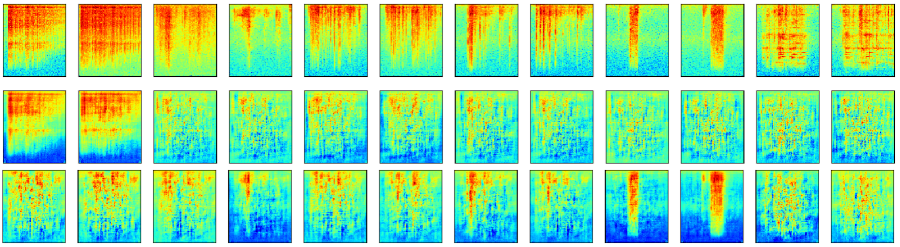
Figure 1: Original (top) and reconstructed (center and bottom) spectrograms using D-PBN. There are two samples of each class in the order “skit”, “sciss”, “pret”, “pens”, “paper”, and “jing”. A description of the sounds is found in [22]. As can be clearly seen, the two rows of reconstructed samples were trained on the first and fifth data class.

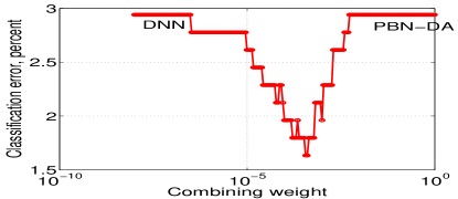
Figure 2: Classifier combination experiment. At the left side, performance with just DNN, and on the right side just PBN-DA.

IV-H D-PBN-DA

To demonstrate the application of deterministic PBN (D-PBN) auto-encoder at high dimension, we trained D-PBN on individual classes by reconstructing the input data from the sixth-layer output (256 dimension) as explained in [9]. There is a 100-fold reduction in dimension. In contrast to previous uses of D-PBN, we applied a discriminative component to the cost function, exactly as done for the PBN-DA. Figure 1 shows examples of reconstructed samples. On the top are a set of 12 original events, two from each class. Below this are seen the reconstructions from the models trained on the first and fifth class. The class correspondence can be easily seen because only data from the target class is well reconstructed. One can classify based on this reconstruction selectivity by choosing the class with lowest reconstruction error. The classifier confusion matrix is (in errors out of 612 samples):

 [102  0   0   0   0   0]
 [ 0  90   1   1  10   0]
 [ 0   2  94   4   2   0]
 [ 0   1   1 100   0   0]
 [ 0   1   2   0  99   0]
 [ 0   0   0   0   0  102]

having 25 errors in 612 samples (4.08% error), almost as good as PBN-DA and DNN. Due to the excellent class selectivity in reconstruction error, the D-PBN-DA has promising potential applications in open-set classification.

V Conclusions

Using some of the dimension mitigation methods proposed in Section III, we were able to effectively apply PBN at an input data dimension of 24,318, much higher than the previously demonstrated dimensions of 900 and 196 (See Figures 4 and 5 in [17]). Furthermore, Figure 2 confirms that the advantages of a discriminatively aligned PBN seen at lower dimensions, (a) PBN-DA working about as well as a state of the art DNN, (b) the combined performance being significantly better that either classifier alone, also apply at higher dimension. In addition, we have demonstrated a novel new auto-encoder classifier (D-PBN-DA) that performs as well as a state of the art CNN on the same high-dimensional data set. The data, software, and instruction for recreating these results are archived at [25].

References

- [1] P. M. Baggenstoss and S. Kay, “Nonlinear dimension reduction by pdf estimation,” (Accepted in) IEEE Transactions on Signal Processing, 2022.
- [2] P. M. Baggenstoss, “The PDF projection theorem and the class-specific method,” IEEE Trans Signal Processing, pp. 672–685, March 2003.
- [3] P. M. Baggenstoss, “Maximum entropy PDF design using feature density constraints: Applications in signal processing,” IEEE Trans. Signal Processing, vol. 63, June 2015.
- [4] M. Rosenblatt, “Remarks on a multivariate transformation,” The Annals of Mathematical Statistics, vol. 23, no. 3, pp. 470–472, 1952.
- [5] G. Deco and W. Brauer, “Nonlinear higher-order statistical decorrelation by volume-conserving neural architectures,” Neural Netw., vol. 8, p. 525–535, June 1995.
- [6] G. Deco and D. Obradovic, AN INFORMATION-THEORETIC APPROACH TO NEURAL COMPUTING. Springer, 1996.
- [7] A. Hyvärinen, J. Karhunen, and E. Oja, Independent Component Analysis. Wiley, 2001.
- [8] A. Hyvärinen and P. Pajunen, “Nonlinear independent component analysis: Existence and uniqueness results,” Neural Networks, vol. 12, no. 3, pp. 429–439, 1999.
- [9] P. M. Baggenstoss, “A neural network based on first principles,” in ICASSP 2020, Barcelona (virtual), (Barcelona, Spain), Sep 2020.
- [10] P. M. Baggenstoss, “Applications of projected belief networks (pbn),” in Proceedings of EUSIPCO 2019, (La Coruña, Spain), Sep 2019.
- [11] P. M. Baggenstoss, “Applications of projected belief networks (PBN),” Proceedings of EUSIPCO, A Corunã, Spain, 2019.
- [12] P. M. Baggenstoss, “The projected belief network classifier: both generative and discriminative,” Proceedings of EUSIPCO, Amsterdam, 2020.
- [13] M. Welling, M. Rosen-Zvi, and G. Hinton, “Exponential family harmoniums with an application to information retrieval,” Advances in neural information processing systems, 2004.
- [14] G. E. Hinton, S. Osindero, and Y.-W. Teh, “A fast learning algorithm for deep belief nets,” in Neural Computation 2006, 2006.
- [15] D. J. Rezende, S. Mohamed, and D. Wierstra, “Stochastic backpropagation and approximate inference in deep generative models,” in Proceedings of the 31st International Conference on Machine Learning (E. P. Xing and T. Jebara, eds.), vol. 32 of Proceedings of Machine Learning Research, (Bejing, China), pp. 1278–1286, PMLR, 22–24 Jun 2014.
- [16] I. Goodfellow, J. Pouget-Abadie, M. Mirza, B. Xu, D. Warde-Farley, S. Ozair, A. Courville, and Y. Bengio, “Generative adversarial nets,” in Advances in Neural Information Processing Systems 27 (Z. Ghahramani, M. Welling, C. Cortes, N. D. Lawrence, and K. Q. Weinberger, eds.), pp. 2672–2680, Curran Associates, Inc., 2014.
- [17] P. M. Baggenstoss, “Discriminative alignment of projected belief networks,” IEEE Signal Processing Letters, Sep 2021.
- [18] V. Vapnik, The Nature of Statistical Learning. Springer, 1999.
- [19] I. Goodfellow, Y. Bengio, A. Courville, and Y. Bengio, Deep Learning. Cambridge, MA: MIT press, 2016.
- [20] S. M. Kay, A. H. Nuttall, and P. M. Baggenstoss, “Multidimensional probability density function approximations for detection, classification, and model order selection,” IEEE Transactions on Signal Processing, vol. 49, pp. 2240–2252, Oct 2001.
- [21] P. M. Baggenstoss, “On the duality between belief networks and feed-forward neural networks,” IEEE Transactions on Neural Networks and Learning Systems, pp. 1–11, 2018.
- [22] P. Baggenstoss, “Office sounds database,” {http://class-specific.com/os}. Accessed: 2022-02-28.
- [23] P. M. Baggenstoss, “Acoustic event classification using multi-resolution hmm,” Proceedings of EUSIPCO 2018, Rome, Sep 2018.
- [24] P. Baggenstoss, “New restricted Boltzmann machines and deep belief networks for audio classification,” 2021 ITG Speech Communication, Kiel (Virtual), 2021.
- [25] P. Baggenstoss, “PBN Toolkit,” {http://class-specific.com/pbntk}. Accessed: 2022-02-28.