An open-source simulation package for power electronics education

Abstract

Extension of the open-source simulation package GSEIM [1] for power electronics applications is presented. Recent developments in GSEIM, including those oriented specifically towards power electronic circuits, are described. Some examples of electrical element templates, which form a part of the GSEIM library, are discussed. Representative simulation examples in power electronics are presented to bring out important features of the simulator. Advantages of GSEIM for educational purposes are discussed. Finally, plans regarding future developments in GSEIM are presented.

1 Introduction

Simulation can be a very effective tool for improving students’ understanding of fundamental concepts since it allows verification of the concepts as well as quick exploration of several “what-if” scenarios. In the context of power electronics, for example, simulation allows the student to view the effect of changing a duty ratio or an inductance value on the voltage and current waveforms in the circuit under discussion, thus reinforcing the concepts being taught in class. Several commercial simulation tools are currently being used for teaching power electronics, including PSIM [2], PSCAD [3], Matlab Simulink/Simscape [4], and PLECS [5]. While academic versions of these packages at a lower cost or free student versions (with limitations) are generally available, open-source options are certainly advantageous, especially for engineering colleges in developing countries.

There are currently few open-source options for power electronics. Of those, Openmodelica [6] is based on the hardware description language Modelica, while GeckoCIRCUIT [7] is a java-based platform. Open-source tools are currently not being used for power electronics education on a large scale probably because of attractive features such as ease of use and customer support associated with commercial packages.

An open-source simulator GSEIM was recently reported [1]. In the first version, GSEIM was aimed at simulation of power electronic systems which can be represented by a flow-graph, e.g., V/f control of an induction motor. Subsequently, GSEIM has been extended, both in terms of GUI features and numerical engine, to enable simulation of a number of power electronic circuits covered in typical undergraduate and postgraduate courses. It is the purpose of this paper to report the current status of the GSEIM package and point out its potential as an open-source tool for power electronics education.

The paper is organised as follows. In Sec. 2, recent developments in GSEIM are reported. The most important development, viz., addition of electrical elements in the form of templates, is described in Sec. 3, with the help of examples. In Sec. 4, simulation examples are presented to bring out the scope and capabilities of the program. Advantages of GSEIM as an open-source package have been pointed out in Sec. 5. Finally, in Sec. 6, conclusions of this work are summarised, and future developments envisaged in GSEIM are listed.

2 Recent developments in GSEIM

The currently available GSEIM program [8] allows the user to enter the schematic diagram of the system of interest using a graphical user interface (GUI), specify component values, run simulation, and plot results interactively. In addition, it allows the user to create new elements (blocks) either in terms of equations or as hierarchical blocks made up of elements already available in the library. Applications are limited to power electronic systems which can be represented as a flow-graph, with each element having input and output nodes. The primary objective of the new GSEIM version presented in this paper is to allow simulation of electrical circuits. For convenience, we will call the new GSEIM version GSEIM-Electrical (GSEIM-E) and the original GSEIM program described in [1] as GSEIM-Flowchart (GSEIM-F). In the following, we summarise the salient features of GSEIM-E.

• Numerical engine: The numerical engine (C++) of the GSEIM-F program was extended to handle electrical elements. The modified nodal analysis (MNA) approach, along with the Newton-Raphson method for nonlinear circuits, was implemented. When the system being simulated has electrical elements, only implicit methods – backward Euler or trapezoidal method with constant or variable time steps – are allowed for numerical integration. The details of these techniques can be found in [9] and references therein.

• Steady-state waveform (SSW) analysis: In several converter applications, the steady-state waveform is of interest. In priniciple, transient simulation performed for a sufficiently large number of cycles can yield the steady-state solution. However, this process can take too long if the circuit time constants are large. The Newton-Raphson time-domain steady-state waveform (NRTDSSW) method described in [10] is implemented in GSEIM-E for directly obtaining the steady-state solution. An example would be presented in Sec. 4.

• Rectilinear wiring and electrical nodes: In GSEIM-F, the GUI was built by making suitable changes in the GNURadio [11] GUI, and like its predecessor, the GSEIM-F GUI allowed only curved wires (using splines). For electrical circuits, rectilinear wires were incorporated in GSEIM-E, and electrical nodes (ports) were added.

• Element symbols: In GSEIM-F, elements (blocks) were displayed using rectangles, with the type of the element appearing inside the rectangle. In GSEIM-E, circuit symbols, such as resistor and capacitor, are also incorporated. A symbol is rendered in the GUI using a python file associated with that symbol. The user can add a new symbol by simply adding a python file with a suitable name, without making any changes in the GUI code.

  Fig. 1 shows the python file associated with the capacitor symbol. The code between #begin_cord and #end_cord prepares the points involved in the symbol, and the code between #begin_draw and #end_draw does the rendering.

  

  Figure 1: Python file associated with the capacitor symbol.

• Plotting: The following post-processing features have been added to the plotting GUI:

  • Average and rms values

  • Fourier spectrum and total harmonic distortion (THD)

In some aspects, GSEIM is similar to SEQUEL [9]. However, the organisation of GSEIM is significantly different. In particular, the SEQUEL library involves both basic and compound elements, whereas the GSEIM library involves only basic elements, the compound elements being treated through the hierarchical block facility provided by the GSEIM GUI. The other important difference is that GSEIM is oriented mainly toward power electronics while SEQUEL is more general.

3 Electrical element templates

As discussed in [1], the equations governing the behaviour of an element is incorporated in GSEIM in the form of “templates.” Some of the flow-graph type element templates have been discussed in [1]. Here, we look at a few electrical basic element (ebe) templates.

• Resistor: Fig. 2 shows the resistor template. The terminal currents are given by $i_{p}\,$=$\,\displaystyle\frac{v_{p}-v_{n}}{R}$, $i_{n}\,$=$\,-\,\displaystyle\frac{v_{p}-v_{n}}{R}$. The derivatives of these functions $\displaystyle\frac{\partial i_{p}}{\partial v_{p}}$, $\displaystyle\frac{\partial i_{p}}{\partial v_{n}}$, etc. are constants, and that is indicated by the Jacobian statement. The nodes and the rparms statements specify the nodes and real parameters of the element, respectively. The outparms statement specifies the quantities made available by this element to the user for plotting.

  

  Figure 2: Resistor template (partial).

  The main program expects three types of functions to be supplied by an electrical element template.

  • Functions $f_{1}$, $f_{2}$, $\cdots$ are related to terminal currents in transient simulation. If the element has $N$ nodes, the first $N$ of these equations give the node currents, while the remaining equations (if any) are auxiliary equations.

  • Functions $g_{1}$, $g_{2}$, $\cdots$ are related to state variables, as we will see with respect to the capacitor template.

  • Functions $h_{1}$, $h_{2}$, $\cdots$ are related to “start-up” simulation, which involves solving the circuit equations while holding state variables such as capacitor voltages and inductor currents constant, at some specified values [9]. For a resistor, there are no state variables, and therefore the $f$ and $h$ equations are identical.

  The statement n_f=2 conveys that there are two $f$ functions for this element. The statements starting with f_1: and f_2: indicate which variables these functions depend on. The main program passes two objects to the template: (a) X which carries information about the specific element being called, and (b) G which carries global information such as the current time point. By checking the flags of G, the template computes appropriate quantities, and passes them to the main program by assigning suitable variables of X. Some flags of G are listed below.

  • i_one_time_parms: compute “one-time” parameters which are not required to be computed in every time step.

  • i_trns: transient simulation

  • i_function: compute function values

  • i_jacobian: compute jacobian values

  • i_outvar: compute output parameters

• Capacitor: A capacitor involves a time derivative and therefore calls for a very different treatment as compared to a resistor. The terminal currents can be written as $i_{p}\,$=$\,\displaystyle\frac{dQ_{p}}{dt}$, $i_{n}\,$=$\,\displaystyle\frac{dQ_{m}}{dt}$, where $Q_{p}\,$=$\,C\,(v_{p}-v_{n})$ and $Q_{m}\,$=$\,-Q_{p}$ are state variables. The functions $f_{1}$, $f_{2}$, $g_{1}$, $g_{2}$ in the capacitor template shown in Fig. 3 are used to implement these equations.

  

  Figure 3: Capacitor template (partial).

  In start-up simulation, the capacitor behaves like a dc voltage source, satisfying the equations, $i_{p}\,$=$\,i_{1}$, $i_{n}\,$=$\,-i_{1}$, and $v_{p}-v_{n}\,$=$\,V_{0}$, where the current $i_{1}$ is an auxiliary variable, and $V_{0}$ is a start-up parameter. Implementation of these equations is shown in the start-up part of the capacitor template (see Fig. 4) where the variable cur_p is used to denote $i_{1}$.

  

  Figure 4: Start-up section of the capacitor template.

4 Simulation examples

We now present a few simulation examples to demonstrate the capabilities of GSEIM-E. As explained in [1], simulation of a circuit with GSEIM-F involves drawing the circuit, assigning component values, setting output variables for plotting, and preparing an appropriate “solve block” to specify parameters related to a specific simulation. This procedure remains the same for GSEIM-E except for minor changes to handle electrical elements. The details would be explained in the on-line GSEIM-E documentation, currently under preparation.

The circuit schematics shown in this section are taken directly from the GSEIM-E GUI, by exporting them to pdf files. Apart from the pdf format, the GSEIM-E GUI, like its predecessor GNURadio, also allows circuit schematics to be exported in svg and png formats. This feature is useful in preparing presentations or reports.

• $V/f$ control of an induction motor: This example has been described in [1]. Here, we show only the schematic diagram as it appears in the GSEIM-E GUI in order to demonstrate some of the new features of the GUI, viz, rectilinear wiring and the use of element symbols.

  

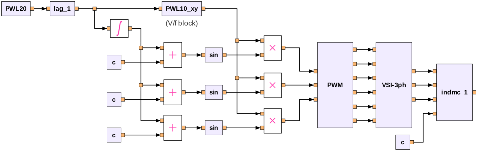
  Figure 5: Schematic diagram for $V/f$ control of an induction motor.

• Buck converter: The buck converter circuit, shown in Fig. 6 was simulated for different values of duty ratio $D$ and inductance $L$. In each case, $i_{L}\,$=$\,0$ A and $v_{C}\,$=$\,0$ V is taken as the starting point. The output voltage $V_{o}(t)$ is plotted in Fig. 7 for three cases.

  

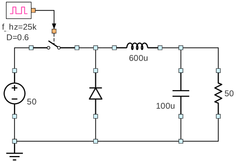
  Figure 6: Schematic diagram of buck converter.

  As seen from the figure, the output voltage takes some time to settle to its steady-state value. Typically, when teaching a power electronics course, the steady-state situation is of interest, and not the trajectory of the circuit to the steady state. Following the transient simulation approach for this circuit – and also several other converter circuits – is therefore wasteful. From Fig. 7, we see that, for the component values specified, the circuit takes about 10 msec or 250 cycles to reach the steady state, whereas only the last one cycle is of interest.

  

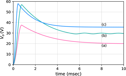
  Figure 7: Output voltage versus time for the buck converter of Fig. 6. (a) $D\,$=$\,0.4$, $L\,$=$\,600\,\mu$H, (b) $D\,$=$\,0.6$, $L\,$=$\,600\,\mu$H, (c) $D\,$=$\,0.6$, $L\,$=$\,200\,\mu$H.

  Furthermore, the time taken to reach the steady state depends on the parameter values and is generally not know a priori. In the classroom, if a teacher wants to demonstrate, for example, continuous and discontinuous conduction by changing $L$ or $C$ or $D$, transient simulation is clearly not a good option, and a method to directly obtain the steady-state solution is desirable.

  GSEIM-E incorporates the Newton-Raphson time-domain steady-state waveform (NRTDSSW) approach described in [10] for steady-state waveform (SSW) computation. GSEIM-E SSW results for the inductor current are shown in Fig. 8 for the same parameter sets as in Fig. 7.

  

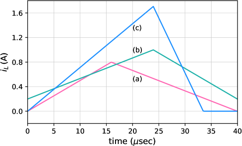
  Figure 8: Steady-state inductor current versus time for the buck converter of Fig. 6. (a) $D\,$=$\,0.4$, $L\,$=$\,600\,\mu$H, (b) $D\,$=$\,0.6$, $L\,$=$\,600\,\mu$H, (c) $D\,$=$\,0.6$, $L\,$=$\,200\,\mu$H.

  To summarise, the SSW approach offers two major advantages over transient simulation: (a) it is much faster, (b) it does not require the user to guess the number of cycles required to reach the steady state. We expect the SSW feature of GSEIM-E to become one of its most useful features for power electronics education. To the authors’ best knowledge, SEQUEL [9] and PLECS [5] are the only other simulation packages with direct SSW computation capability in the context of power electronic circuits.

• Neutral point clamped inverter: Fig. 9 shows the schematic diagram of a neutral clamped inverter. The clock generation blocks and the switch-diode blocks are implemented using subcircuits (hierarchical blocks). For this circuit, the Fourier spectrum of the load current is of interest. Fig. 10 shows the spectrum for the load current, as obtained with GSEIM’s plotting GUI.

  

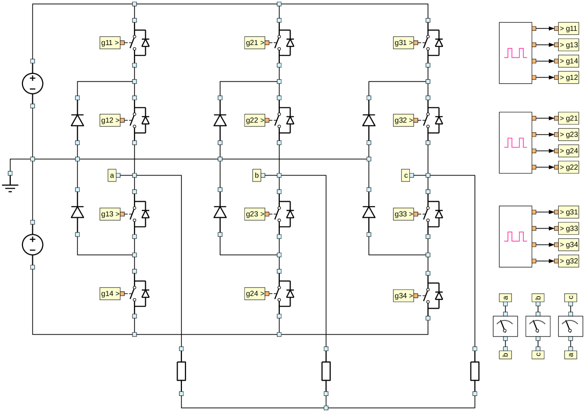
  Figure 9: Schematic diagram of neutral point clamped inverter.

  

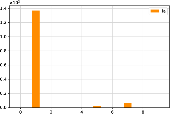
  Figure 10: Fourier spectrum for neutral point clamped inverter of Fig. 9.

The above examples, together with the machine control examples presented in [1], represent the current focus and scope of GSEIM. We have been able to perform simulation speed comparison for a set of problems involving electrical machines. We found GSEIM to be 2 to 5 times faster than Simulink in this study [12]. A more detailed comparison with Simulink/Simscape and other commonly used commercial packages is planned; the results will be presented elsewhere.

5 GSEIM as an open-source package

The examples presented in Sec. 4 bring out the potential of GSEIM in teaching power electronics courses. Furthermore, the open-source nature of GSEIM is advantageous in several ways:

• Vendors of commercial packages are constrained from revealing several implementation details. As a result, their documentation is mostly about “know-how” rather than “know-why”. Creators of open-source packages are not limited by the need for intellectual property protection and can therefore afford to make their documentation richer and academically far more rewarding for the users.

  As an example, consider the thyristor block from Simscape [13] as shown in Fig. 11. The purpose served by the inductor $L_{\mathrm{on}}$ is not explained. Apart from that, consider the following statements in the documentation for this block:

  • “The Inductance Lon parameter is normally set to 0 except when the Resistance Ron parameter is set to 0.”

  • “The Thyristor block cannot be connected in series with an inductor, a current source, or an open circuit, unless its snubber circuit is in use.”

  From the user’s perspective, these statements appear esoteric and create the (wrong) impression that circuit simulation is very complex. On the other hand, if the reasons behind these limitations were explained, it would have led to a far better understanding of the simulation process.

  

  Figure 11: Thyristor block from Simscape [13].

• Contributions from users to library elements and simulation examples can be easily incorporated in an open-source package like GSEIM. Indeed, the basic philosophy behind open-source packages is user involvement in not only using the package but also its continuous evolution. In the development of GSEIM, special care has been taken in order to allow users’ contribution in terms of new basic elements, element symbols, hierarchical blocks (subcircuits), simulation examples as well as documentation, with the hope that the package will grow into a valuable resource for power electronics education.

• Commercial packages often tend to hide, apart from implementation details, even data files created by the package, thus forcing the user to use a commercial tool – generally a part of the same package – for viewing the results. Open-source packages on the other hand are generally designed keeping in mind free exchange of the output files generated by the package in ASCII or csv format, for example. GSEIM creates output files in ASCII format, and they can be viewed not only with the plotting GUI provided with GSEIM, but also with any other plotting program including open-source programs like gnuplot and matplotlib.

• Students in several engineering colleges, particularly in developing countries, cannot afford licenses for commercial packages. As a consequence, teachers are unable to assign home-work exercises involving simulation, and students are deprived of the precious learning experience offered by simulation. Open-source packages completely remove this constraint since no licenses are involved.

• Open-source packages can take advantage of other open-source tools such as compilers, libraries, and plotting programs. This can lead to improved capabilities, performance, and implementation.

• Open-source packages can be combined with other open-source packages to create new capabilities at no cost to the user. For example, GSEIM can be easily called by an optimisation package for circuit design.

  On the other hand, if two commercial packages are combined, the user has to pay for each of them, e.g., see [14].

6 Conclusions and future plans

GSEIM, an open-source simulation package for power electronics education, has been presented in this paper. The organisation and features of GSEIM have been described. Incorporation of new elements in the GSEIM library has been discussed with the help of specific examples. A few simulation examples have been considered to illustrate the potential of GSEIM in power electronics education. Future plans for GSEIM include the following.

• manual preparation and uploading of the revised GSEIM version on github [8]

• video tutorials for new users

• course material development based on GSEIM simulation examples

• additional features such as “bus” connections, real-time plotting of simulation results.

References

- [1] M. B. Patil, R. D. Korgaonkar, and K. Appaiah, “GSEIM: a general-purpose simulator with explicit and implicit methods,” Sādhanā, vol. 46, no. 4, pp. 1–13, 2021.
- [2] PSIM. [Online]. Available: https://powersimtech.com/products/psim/capabilities-applications/
- [3] PSCAD. [Online]. Available: https://www.pscad.com/
- [4] Simulink – Simulation and Model-Based Design. [Online]. Available: https://in.mathworks.com/products/simulink.html
- [5] PLECS. [Online]. Available: https://www.plexim.com/products/plecs
- [6] OpenModelica. [Online]. Available: https://openmodelica.org/
- [7] A. Müsing and J. W. Kolar, “Successful online education-geckocircuits as open-source simulation platform,” in 2014 International Power Electronics Conference (IPEC-Hiroshima 2014-ECCE ASIA). IEEE, 2014, pp. 821–828.
- [8] GSEIM. [Online]. Available: https://github.com/gseim/gseim
- [9] M.B. Patil. SEQUEL Users’ Manual: Part-1. [Online]. Available: http://www.ee.iitb.ac.in/~sequel
- [10] M. B. Patil, M. C. Chandorkar, B. G. Fernandes, and K. Chatterjee, “Computation of steady-state response in power electronic circuits,” IETE journal of research, vol. 48, no. 6, pp. 471–477, 2002.
- [11] GNU Radio Manual and C++ API Reference. [Online]. Available: http://www.gnuradio.org
- [12] A. Nandan and M. Patil, “Comparison of GSEIM with Simulink with respect to simulation speed,” in International Conference on Signal Processing, Informatics, Communication and Energy Systems. IEEE, 2022.
- [13] Thyristor. [Online]. Available: https://in.mathworks.com/help/physmod/sps/powersys/ref/thyristor.html
- [14] PLECS Blockset. [Online]. Available: https://www.plexim.com/download/blockset