Rheology of Pseudomonas fluorescens biofilms: from experiments to DPD mesoscopic modelling

Abstract

The presence of bacterial biofilms in clinical and industrial settings is a major issue worldwide. A biofilm is a viscoelastic matrix, composed of bacteria producing a network of Extracellular Polymeric Substances (EPS) to which bacteria crosslink. Modelling of complex biofilms is relevant to provide accurate descriptions and predictions that include parameters as hydrodynamics, dynamics of the bacterial population and solute mass transport. However, up-to-date numerical modelling, even at a coarse-grained level, is not satisfactorily. In this work, we present a numerical coarse-grain model of a bacterial biofilm, consisting of bacteria immersed in an aqueous matrix of a polymer network, that allows to study rheological properties of a biofilm. We study its viscoelastic modulus, varying topology and composition (such as the number of crosslinks between EPS polymers, the number of bacteria and the amount of solvent), and compare the numerical results with experimental rheological data of Pseudomonas fluorescens biofilms grown under static and shaking conditions, as previously described by Jara et al, Frontiers in Microbiology (2021).

I Introduction

Biofilms are synergistic colonies of one or more bacterial species growing on a solid surface most often in contact with an aqeuous liquid. In contrast to liquid-floating planktonic bacterial cells, bacteria embedded in solid-supported biofilms do not have unlimited access to nutrients. The presence of biofilms does not only provide the physical protection of the embedded cells against chemical or mechanical challengesPeterson et al. (2015); Flemming and Wingender (2010), but it also facilitates the evolution of phenotypes that eventually lead to the resistance to the treatment of antimicrobial agents Donlan (2001a); Hoiby et al. (2010). Antimicrobial resistance of bacteria dwelled in biofilms compromises the process of bacterial removal giving rise to a more persistent bacterial infection. Reason why biofilm formation is a major health issue Khatoon et al. (2018); Milchev and Binder (2013) and industrial challenge worldwide Duan et al. (2008); Mansour and Elshafei (2016); Schultz and Swain (2000). Bacterial infections in plants and animals lead to food contamination and poisoningZhao et al. (2016) . A biofilm is a complex and heterogeneous viscoelastic material J.N.Wilking et al. (2011) produced by bacterial cells. In more structural terms, a biofilm consists of a network of extracellular polymeric substances (EPS) composed of polysaccharides, proteins, extracellular DNA, and cells, everything surrounded by an aqueous environment. EPS serves as a scaffold for matrix cross-linked bacterial cells embedded within the biofilm. The amount of bacteria with respect to EPS vary from one tenth to one fourth of the total biofilm massGarrett et al. (2008); Sveinbjörnsson et al. (2012), depending on the bacterial species. Mathematical modelling of bacterial biofilms started more than 30 years ago Klapper and Dockery (2010); Wang and Thanou (2010). Biofilms have been described via phase-field (continuum) models, in which one phase represented the biofilm (EPS and bacteria) and the other phase the surrounding matrix containing the nutrient substrates Zhang et al. (2008). The tension and compression of a biofilm have been computed using finite elements simulations to obtain the Young’s modulus of an artificial biofilm composed of bacteria embedded in an agarose hydrogel Kandemir et al. (2018).

A different approach consisted in implementing an hybrid discrete-continuum models to incorporate the flow of substrate, bacterial growth or biomass spreading over the rough biofilm surfaces Picioreanu et al. (1999, 2004). More recently, mesoscale numerical models such as the immersed boundary-based method (IBM) or the dissipative particle dynamics (DPD) have been proposed to study biofilm maturation Horn and Lackner (2014); Eberl et al. (2008); Liu and Balazs (2018a); Xu et al. (2011a), establishing a connection between the mechanical stress and strain of the biofilm Bol et al. (2012); Hammond et al. (2014a); Stotsky et al. (2016a). On the one side, to model a complex system via the IBM model Peskin (1977, 2002) several assumptions need to be taken into account, such as 1) not considering biofilm growth but steadiness during the simulation time scale Hammond et al. (2014b), 2) mimicking biofilm elasticity via linear springs that connect individual bacterial cells Stotsky et al. (2016b) and 3) capturing the biofilm viscosity via constitutive equations for stress. As a matter of phenomenological evidence, macroscopic rheological experiments were considered on Staphylococcus epidermidis biofilms grown on a plate rheometer Pavlovsky et al. (2013). They were compared qualitatively to numerical results obtained via the microscale spatial IBM model Stotsky et al. (2018). On the other side, as refers to dynamic methods Barai et al. (2016), DPD conserve mass and momentum under steady state conditions. Differently from grid-based computational methods that do not consider any mechanical constraints, DPD can be easily implemented when considering objects with complex geometries Xu et al. (2011b). Like Molecular Dynamics (MD) simulations Mukhi and Vishwanathan (2021), DPD captures the time evolution of a many-body system with friction explicitly considered. Unlike MD, DPD allows to model physical phenomena occurring at longer time scales and length scale Raos and Casalegno (2011). DPD was thus implemented to simulate biofilm formation on post-coated surfaces Liu and Balazs (2018b), and the growth of two-dimensional biofilm in flow Xu et al. (2011c). Recently, we have presented a combined numerical and experimental study on how hydrodynamic stress affect structural features of Pseudomonas fluorescens biofilms Jara et al. (2021). By means of rheological measurements on a biofilm grown in the presence and in the absence of hydrodynamic stress, we demonstrated that bacteria are capable of adapting to hostile deformations by tailoring the structure of the matrix and its viscoelastic properties Jara et al. (2021). The results were supported by numerical results of the rheological properties of a mimetic biofilm simulated as a first approximation via a DPD model. Thanks to computer simulations, we learned that biofilms grown under stress were mechanically more stable due to an increase of the number of crosslinks between EPS polymers.

In this work we probe the rheological features of a P. fluorescens biofilms varying the frequency of the externally imposed shear flow. To numerically study the biofilm viscoelastic modulus, we use a coarse-grain DPD model. To better characterised the biofilm, we vary topology and composition parameters such as the number of matrix crosslinks between EPS polymers, the number of bacteria embedded and the amount of solvent. The numerical results are compared to experimental rheological data of P. fluorescens biofilms grown under static and shaking conditions.

II Numerical and experimental details

In what follows, we present the mesoscopic model used to simulate mature biofilms, and the experimental details of the viscoelastic measurements of a P. fluorescens biofilm.

II.1 Mesoscopic model for an in silico biofilm

The simulated biofilm consists of three different components: bacteria, polymers and solvent. The biofilm is prepared in an initial configuration consisting of a colony of monodisperse bacteria immersed in a periodic box containing solvent and randomly distributed polymers.

II.1.1 Bacteria

Differently from the work described by Raos et al.Guido et al. (2006), where dispersed filler particles aggregated into a single bacterium, we use realistic bacteria consisting of already clustered particles. We model the bacterium as a bacillus (rod-shaped) composed by 440 particles (of type $b$), each of diameter $\sigma_{b}$, held together via harmonic interactions.

$$U_{b}^{\rm bond}=\frac{K_{b}}{2}(r_{i,j}-\sigma_{b})^{2}\qquad,$$ (1)

being $r_{i,j}$ the distance between the bonded beads $i$ and $j$, $\sigma_{b}$ the equilibrium distance, $K_{b}$ the harmonic coupling constant. The central part of a bacterium is shaped as an empty cylinder of length $l_{b}/\sigma_{b}=6$, while the extremes of the bacteria are shaped as spherical caps of radius $R_{ext}/\sigma_{b}=4$. Both the central and extreme parts have an external radius $R_{ext}/\sigma_{b}=4$ and internal radius $R_{ext}/\sigma_{b}=2$, i.e. the bacterium membrane is formed by three layers of particles.

II.1.2 Matrix: polymers and solvent

The bacteria are immersed in a bulk matrix made of polymers (EPS) and solvent. The solvent is represented by $N_{\rm solv}$ particles of type $s$, whereas the EPS is represented by linear chains of $l$ beads of type $p$ that are bound via harmonic potential:

$$U_{p}^{\rm bond}=\frac{K_{p}}{2}(r_{i,j}-\sigma_{p})^{2}\qquad,$$ (2)

where $r_{i,j}$ is the distance between two consecutive beads $i$ and $j$, $\sigma_{p}$ the equilibrium distance, and $K_{p}$ the coupling constant.

II.1.3 Cross-links and non-bonded interactions

The crosslink (CL) interactions, occurring between two beads of type $p$ (polymer-polymer crosslink), or between beads of type $b$ and $p$ (bacterium-polymer crosslink), are described via harmonic potential:

$$U^{\rm CL}=\frac{K}{2}(r_{i,j}-\sigma_{CL})^{2}\qquad.$$ (3)

All non-bonded interactions, namely polymer-polymer (pp), polymer-bacterium (pb), polymer-solvent (ps), bacterium-bacterium (bb), bacterium-solvent (bs), and solvent-solvent (ss) interactions, are modelled according to the DPD force field. In particular, the force between two particles $i$ and $j$, respectively of type $\alpha$ and $\beta$, is expressed as the sum of a conservative force $\vec{F}^{C}_{i,j}$, a dissipative force $\vec{F}^{D}_{i,j}$ and a random force $\vec{F}^{R}_{i,j}$ given by

$$\vec{F}^{C}_{i,j}=B_{\alpha,\beta}w(r)\hat{r}_{i,j}\qquad r<r_{c}$$ (4)

where $r_{c}$ is the cut-off distance, beyond which all the terms vanish; $\hat{r}_{i,j}$ is the unit vector along the direction of the vector $\vec{r}_{i}-\vec{r}_{j}$, indicating the positions of particles $i$ and $j$, respectively; $B_{\alpha,\beta}$ is the amplitude of the conservative force between particles of type $\alpha$ and $\beta$;

$$\vec{F}^{D}_{i,j}=-\gamma w^{2}(r)\left(\hat{r}_{i,j}\cdotp\hat{v}_{i,j}\right)\hat{r}_{i,j}$$ (5)

where $\vec{v}_{i,j}\equiv\vec{v}_{i}-\vec{v}_{j}$ is the vector difference between the velocity $\vec{v}_{i}$ of particles $i$, and the velocity $\vec{v}_{j}$ of particle $j$; $\gamma$ the friction coefficient;

$$\vec{F}^{R}_{i,j}=w(r)\left(\dfrac{2k_{B}T\gamma}{dt}\right)^{1/2}\Theta\,\,\,\hat{r}_{i,j}$$ (6)

$$w(r)=1-r/r_{c}$$ (7)

Here, $w(r)$ is a weighting factor varying from 0 to 1; $\Theta$ is a Gaussian random number with zero mean and unit variance; $dt$ the integration time; $k_{B}$ the Boltzman constant; $T$ the absolute temperature. The sum of the three DPD forces allows to capturing the long-range correlations induced by the hydrodynamic interactions, also accounting for thermal fluctuations.

II.2 Numerical details

We simulated the biofilm via the LAMMPS open source codePlimpton (1995). The system evolves according to a velocity Verlet algorithm, keeping fixed the volume of the simulation box, set to $32\times 32\times 32$ with periodic boundary conditions. We simulate the biofilm changing the number of bacteria $N_{b}$ from 90 to 184, the number of polymers $N_{p}$ (from 80 to 240), the polymer lengths $l$ (from 50 to 200) or the number of solvent particles $N_{s}$ (from 35000 to 75000). All parameters $N_{p}$, $N_{s}$ and $N_{b}$ are chosen to guarantee the DPD condition for the densityHoogerbrugge and Koelman (1992); Groot and Warren (1997): $(N_{p}+N_{b}+N_{s})/(32\times 32\times 32)>3$. Using internal units, we set $r_{c}=1$ for all DPD interactions, $\sigma_{b}=\sigma_{p}=0.5$, $\gamma=4.5$, $K_{b}=K_{p}=30$. The time step is set to $dt=0.05$, although we tested our results also against $dt=0.005$. Moreover, to guarantee that bacteria and polymers are properly hydrated, we choose the amplitudes of the solvent interactions in eq.4 smaller than the remaining ones. In particular, we choose $B_{s,s}=B_{s,b}=B_{s,p}=25$ and $B_{b,b}=B_{p,p}=B_{p,b}=30$. To convert those dimensionless units in real world units, we consider $k_{B}T=4.11\times 10^{-21}$ J as the characteristic energy scale in our simulation. Also, we set the system length scale to the longest dimension of one P. fluorescens bacterium, which can be considered as approximately $\sim 1.5\mu$m. In our simulation the bacterium is 15 beads long, which results in a unit length corresponding to $l_{u}\sim 200$ nm (hence $\sigma_{b}=\sigma_{p}\sim 100$ nm). Moreover, since the mass of a single bacterium is $\sim 10^{-15}$ Kg, the mass of a single particle is set to $m_{u}\sim 2.3\times 10^{-18}$ Kg. The time scale is derived accordingly as $\tau_{\rm intrinsic}=\sqrt{m_{u}l_{u}^{2}/k_{B}T}\sim 5\times 10^{-6}$s. At a time step of dt=0.01, a period of T=200 corresponds to 2000 time steps that is within the total lifespan of the simulation runs.

II.3 Setting up the initial configuration

We first choose the parameter space to explore. By fixing $N_{b}$, $N_{p}$, $l$ and $N_{s}$, we equilibrate the system in the absence of polymer cross-links (CL) for $\sim 8\times 10^{6}$ time steps and perform simulations changing the parameters within the following ranges: $N_{b}=$ 110, 120, 130, 140, 150, 160, 175, 184, 190, 195; $N_{p}=$ 50, 70, 80, 90, 110, 140, 170; $N_{s}=$ 20000, 30000, 35000, 40000, 50000, number of CL=100, 300, 500, 700, 900, 1100, 1300, 1500, 1700, 2000, 2300, 2400, 2800, 3000, 3200, 3300, 3600, 3800, 4000, 4300, 4400, 4800, 5300, 6000, 7000.

Having prepared the initial configuration, we need to locate the crosslinks within the polymer network. To create the network of cross-linked polymers and bacteria, we randomly place $N_{\rm CL}$ new harmonic bonds 1) between $b$ and $p$ types of particles, i.e. a bacterium-polymer CL and 2) between two $p$ particles (belonging or not to the same polymer chain), i.e. a polymer-polymer CL. To avoid crosslinks agglomerating between nearest neighbours, leading to a clump of $p$ particles of the same polymer chain, we forbid CL between the ten closest neighbors along the same chain. Therefore, we fix the intermolecular distance of the polymer loops within one polymer (intra) or between different polymers (inter) to be at least 10 $\sigma$ apart. To prevent the formation of too many cross-links per particle which would result in a globule-like clusters of beads, we assume that any particle of type $b$ can form at most one CL, while any $p$ particle can form at most two CL. For any choice of $N_{b}$, $N_{p}$, we create an initial configuration and form a number of CL ranging from 2300 up to 5400. After the formation of the CLs, a second equilibration run of $\sim 10^{6}$ time steps is performed to relax the polymer-bacteria network. A characteristic snapshot of the biofilm is shown in Fig. 1.

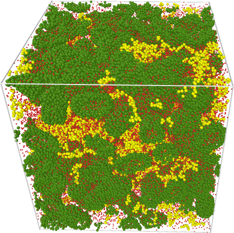
Figure 1: Snapshots of the simulation box containing 184 bacteria (in green), 80 polymers (in yellow) and 35000 solvent particles (in red). The size of a single particle has been chosen for the sake of visualization and does not reflect the interaction radius.

II.4 Simulated rheology: numerical details

To study the rheological properties of the biofilm, we compute the shear modulus by monitoring the shear stress response $\sigma(t)$ under a sinusoidal deformation. We apply an external oscillatory shear deformation with frequency $\nu$ along th $X$–$Y$ plane by changing the box size $L_{z}$Raos and Casalegno (2011); Jara et al. (2021) according to

$$L_{z}(t)=L_{0}+A\sin(2\pi\nu t)\qquad,$$ (8)

being $L_{0}=32$ the initial box size and $A$ the amplitude of the oscillation. Under shearing conditions, the particle velocities are remapped every time they cross periodic boundaries. Within our simulations, we have explored the following values for the amplitude $A$ :A= 2.5, 3.2, 4.8, 8, 12, 16, 20, 24, 28, 32, 36; and the period $T$: T$\equiv\frac{2\pi}{\nu}$= 20, 50, 100, 200, 500, 1200, 2000, 2500, 5000, 10000, 20000, 100000, 200000.

According to Raos et al. Guido et al. (2006), the resulting stress has been calculated by fitting the $xy$ component of the shear stress with:

$$\sigma_{xy}(t)=\sigma^{\prime}\cdot\sin(2\pi\nu t)+\sigma^{\prime\prime}\cdot\cos(2\pi\nu t)$$ (9)

and the amplitude values of $\sigma^{\prime}$ and $\sigma^{\prime\prime}$ were used to compute the the in-phase and out-of-phase components of the complex shear modulus

$$G^{\prime}=\frac{\sigma^{\prime}}{(A/L_{0})}\qquad G^{\prime\prime}=\frac{\sigma^{\prime\prime}}{(A/L_{0})}$$ (10)

being $G^{\prime}$ the storage modulus and $G^{\prime\prime}$ the loss modulus, respectively. Rheological properties of solid biomaterials are characterized by a finite storage modulus $(G^{{}^{\prime}}>0$). Whereas fluid viscous materials are characterized by near zero storage modulus $(G^{{}^{\prime}}\sim 0$) and a large loss modulus $(G^{{}^{\prime\prime}}>0$)Donlan (2001b); Alonci et al. (2018).

From a phenomenological point of view, the computed stress-strain curves are mainly characterized by two regimes a) The stress-strain curves are linear at low strain, where the stress is proportional to the the strain. b) Beyond a yield strain, where the stress-strain curves deviate from the linear regime. Both regimes crossover at the yield point, which fixes the yield strain in which the system softens becoming effectively plastic.

For the considered frequency ranging from a value of $3\times 10^{-5}$ to a value of $0.3$ (in internal units), we run the simulations completing at least 3 box-shearing oscillations. We consider simulations amplitudes $A$ (ranging from 4 to 36), corresponding to a deformation of up to the 112% of the box size. However, we will mainly focus on data obtained for $A=24$ (75%), since: the stress-strain curve is linear until around a deformation of 50% and starts being non linear for a larger deformation; when varying all parameters ($N_{b}$, $N_{p}$, …) while the behaviour of $G^{{}^{\prime}}$ and $G^{{}^{\prime\prime}}$ is not strongly affected by the choice of A, their response is stronger and the noise lower for $A=75\%$. Thus, we have considered a period $T$ ranging from $2\times 10$ to $2\times 10^{5}$.

II.5 Experimental details: Microorganisms and growth conditions

The strain P. fluorescens B52, originally isolated from raw milk Richardson and Te Whaiti (1978), was used as model microorganism. Overnight precultures and cultures were incubated at 20^∘C under continuous orbital shaking (80 rpm) in tubes containing 10 ml Trypticase Soy Broth (TSB, Oxoid). Cells were recovered by centrifugation at 4,000 x g for 10 min (Rotor SA-600; Sorvall RC-5B-Refrigerated Superspeed Centrifuge, DuPont Instruments) and washed twice with sterile medium. Cellular suspensions at OD₆₀₀ were first adjusted to 0.12 (equivalent to 10⁸ cfu/ml) and then diluted to start the experiments at 10⁴ cfu/ml.

II.6 Experimental details: Biofilm development

Biofilms were developed using borosilicate glass surfaces ($20\times 20$ cm) as adhesion substrate. Five glass plates were held vertically into the sections of a tempered glass separating chamber provided with a lid. The whole system was heat-sterilized as a unit before aseptically introducing 2 mL of the inoculated culture medium. To check the effect of hydrodynamic stress on biofilm mechanical properties, incubation was carried out for 96 h at 20^∘C both in an orbital shaker at 80 rpm (shaken sample) and statically (static sample). For biofilm recovery, plates were aseptically withdrawn, rinsed with sterile saline in order to eliminate weakly attached cells and then scraped to remove the attached biomass (cells + matrix) from both faces of the plates. For rheology measurements, biofilm material was casted every 24 h to be directly poured onto the rheometer plate. Experiments were run in triplicate.

II.7 Experimental rheology

As previously described Jara et al. (2021), the viscoelastic response was determined in a hybrid rheometer under oscillatory shear stress-control (Discovery HR-2, TA instruments). We used a cone-plate geometry (40 mm diameter) and a Peltier element to control the temperature through an external an external water thermostat. Measurements were performed at a 1 mm gap between the Peltier element and the plate tool (TA instruments), where a sinusoidal strain $\gamma$ of amplitude $\gamma_{0}$ was performed at a frequency $\omega$, as $\gamma(t)=\gamma_{0}sin(\omega t)$. The shear stress exerted on the biofilm was monitored as $\sigma(t)=G^{*}\gamma(t)$, where $G^{*}$ is the viscoelastic modulus $G^{*}=G^{{}^{\prime}}+iG^{{}^{\prime\prime}}$, where $G^{{}^{\prime}}$ is the storage modulus accounting for shear rigidity, $G^{{}^{\prime\prime}}$ is the loss modulus accounting for viscous friction. These properties were considered under the same definitions as in Eq. (10).

III Results

III.1 Matching the parameters of the biofilm model

To start with, we study the stress response of the biofilm containing cross-linked polymer loops regardless of their intermolecular distances along the polymer chain. We analyze how parameters affect the in-phase ($G^{{}^{\prime}}$) stress response function. In Fig. 2 we represent the storage modulus $G^{{}^{\prime}}$ as a function of the shear amplitude, keeping fixed $N_{b}=150$, $N_{p}=80$, $T=2\times 10^{5}$, $l=100$ and the total number of $CL=1600$ cross-links ($N_{CL,pp}+N_{CL,pb}$).

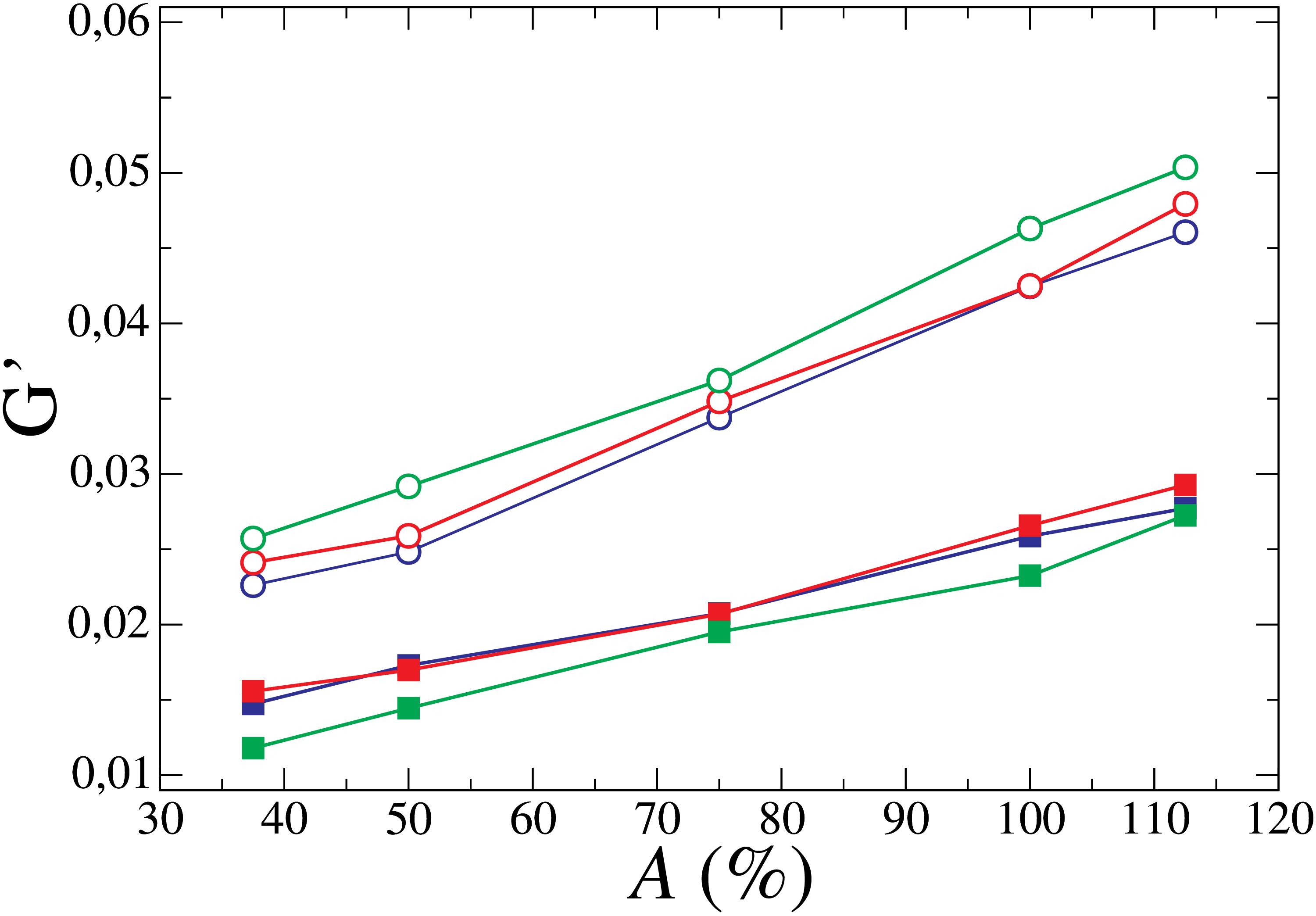
Figure 2: Storage Modulus as a function of the amplitude for different cross-link topologies in the presence (filled squares) and absence (empty circles) of polymer loops. The color code indicates different numbers of polymer-polymer (pp), polymer-bacteria (pb) cross-links: $N_{CL,pp}$ =200/ $N_{CL,pb}$=1400 (blue); $N_{CL,pp}$ =400/ $N_{CL,pb}$=1200 (red) and $N_{CL,pp}$ =600/ $N_{CL,pb}$=1000 (green). All data refer to $N_{b}=150$, $N_{p}=80$, $N_{s}=45000$ and $T=2\times 10^{5}$.

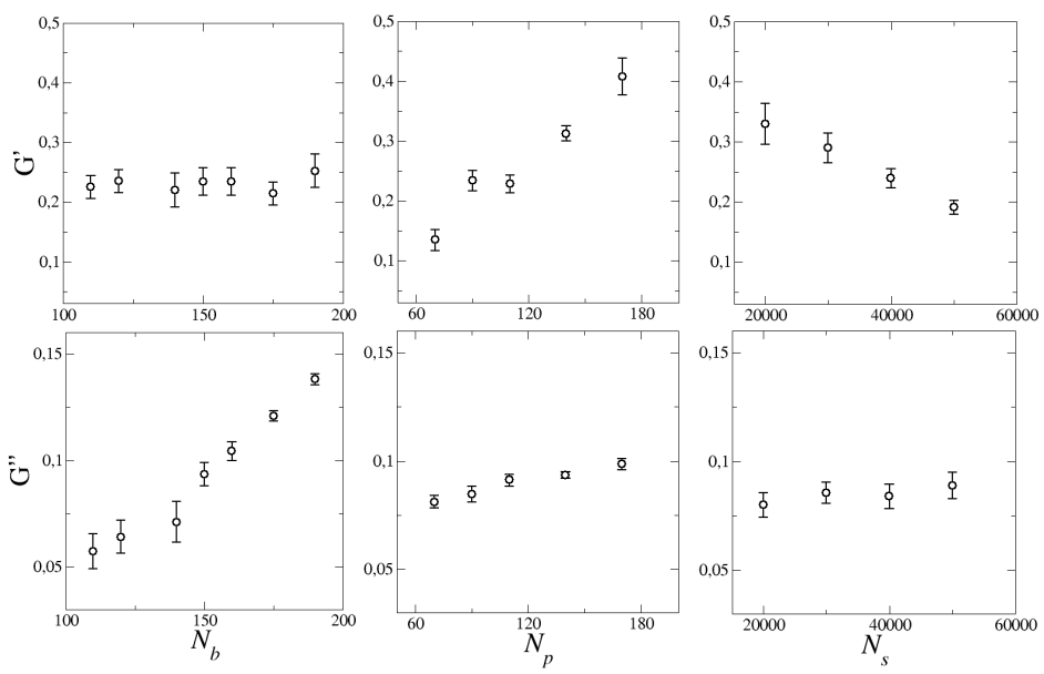
Figure 3: Stress components $G^{\prime}$ and $G^{\prime\prime}$ for $A=75\%$, $CL=2300$ and $T=200$ as function of (a,d) the number of bacteria $N_{b}$; (b,e) the number of polymers $N_{p}$ and solvent (c,f).

We consider two systems with different cross-link topologies: one with polymer cross-links (filled squares) and one without polymer cross-links (empty circles). The presence of polymer loops between $p$ particles belonging to the same polymer chain affects the storage modulus. Since $G^{\prime}$ of the cross-linked biofilm (filled squares, in Fig.2) is lower than the one of the cross-linked biofilm that does not include polymer loops (Fig.2, empty symbols).

This finding indicates the importance to include polymer loops with a biofilm model. As expected, independently of the presence (or absence) of polymer loops, the storage modulus increases with the strain-amplitude. In the presence of polymer loops (for the chosen fixed parameters), we observe that the shear response is not affected by the ratio between polymer-polymer ($pp$) versus polymer-bacteria ($pb$) cross-links. On the other hand, when polymer loops are not present within the same polymer chain, the system response increases (empty symbols in Fig. 2). We think that this increase in system response is due to the presence of a larger number of interactions (connections) between bacteria and matrix polymers. This leads to a a denser and stiffer biofilm and as a consequence generates a larger response function.

III.2 The shear stress dependence on $N_{b}$, $N_{p}$ and $N_{s}$

To check whether the shear stress depends on the number of bacterial cells ($N_{b}$), in Fig. 3, panel a)we study the $G^{{}^{\prime}}$ (in-phase) and $G^{{}^{\prime\prime}}$ (out-of-phase) response as a function of $N_{b}$ (fixing all other parameters). We use an intermediate number of cross-links ($CL=2300$), and intermediate values $N_{p}=80$, $l_{p}=100$, $N_{s}=35000$ within the explored range. Moreover, we apply a deformation amplitude of $A=75$ $\%$ and a period of the deformation of $T=200$. Fixing the different oscillation’s periods to $T=2\times 10^{2}$, we observe a relevant response of $G^{{}^{\prime\prime}}$. Whereas at lower frequencies we have found an amplitude ($A$) depending limiting value of $G^{{}^{\prime\prime}}$ (as we will also observe later in Fig 4).

Our results show that the in-phase response (accounting for the storage, or rigidity modulus $G^{{}^{\prime}}$) remains constant through of the $N_{b}$ range (Fig. 3, panel a). This result is in agreement with previously reported data J.N.Wilking et al. (2011). Considering the bacterial biofilm as a polymer-colloid viscoelastic medium J.N.Wilking et al. (2011), $G^{{}^{\prime}}$ should increase with the bacterial density until reaching a solid-like plateau. Beyond this point, the system behaves as a viscous (liquid-like) fluid. Our findings point out that the probed $N_{b}$-range falls into the elastic response regime, where $G^{{}^{\prime}}$ is not affected by $N_{b}$.

The loss modulus $G^{{}^{\prime\prime}}$ increases linearly with $N_{b}$ (Fig.3, panel d), reflecting the high friction imposed on the system by dragging the large bacteria while increasing their density. The viscous loss almost reaches the values of the storage modulus for the largest number of bacteria considered. However, since $G^{{}^{\prime\prime}}$ is always smaller than $G^{{}^{\prime}}$, the biofilm system behaves as a pasty material, with a relative high structural rigidity $G^{{}^{\prime}}>G^{{}^{\prime\prime}}$ instead of a viscous fluid where $G^{{}^{\prime}}=0$ and $G^{{}^{\prime\prime}}>0$. Thus our model shows a rheological behavior of a quite resilient material with a relatively high mechanical compliance.

To visualize the effect of an increasing number of entangled polymers on the shear response, we consider $N_{b}=150$, $l_{p}=100$, $N_{s}=35000$, $CL=2300$ with an amplitude of $A=75$ $\%$ and period of the deformation of $T=200$ as boundary conditions for our simulations (Fig.3, panel b and e). When we increase the number of polymers and maintain a constant bacterial density, we observe that it is easier for the biofilm to generate a solid-like network with an increased rigidity (Fig.3b). This suggests that bacteria colonize a preexisting polymer template and modify it according to their necessities. The out-phase stress response increases with increasing number of polymers (Fig.3 e) or solvent (Fig.3 f) present in the biofilm. Since this the increase of $G^{{}^{\prime\prime}}$ is quite small when compared to the response caused by the presence of bacteria (Fig.3 d), we consider $G^{{}^{\prime\prime}}$ for polymer and solvent to be constant.

When studying the mechanical response of the system for different hydration levels ($CL=2300$, $N_{b}=184$, $N_{p}=80$, $l_{p}=100$ with an amplitude of $A=75$ % and deformation period of $T=200$), we observe that with increasing number of solvent particles, the biofilm is fully hydrated and the storage modulus decreases (Fig. 3c). This is rather expected as under these experimental conditions the average distance between bacteria and polymers increases and the network becomes mechanically fragile (shear softening). As clearly observed from the data, the biofilm model is able to absorb the solvent. The more solvent is present, the softer the storage modulus (Fig 3c). On the other side, the hydration level seems not to affect $G^{{}^{\prime\prime}}$, which only slightly increases. This softening is not reflected in the loss modulus that remains more or less constant over the tested frequencies (Fig 3d). This implies that the present cross-linked matrix polymers might be entangeled, which allows expansion of the biofilm but at the same time provides rigidity.

III.3 Shear stress dependence on the shearing frequency: simulations versus experiments

Finally, we investigate the stress response as a function of the frequency of the sinusoidal shearing strain $\omega$. On the one side, we perform a rheology experiment on a P. fluorescens biofilm. We grow two P. fluorescens biofilms for 24 hours: one under static conditions, and the second one under shaking conditions. Next, we locate the biofilm ex vivo in the rheometer and measure $G^{{}^{\prime}}$ (filled symbols in Fig.4, top panel) and $G^{{}^{\prime\prime}}$ (empty symbols in Fig.4, top panel) for the static biofilm (Fig.4, top panel, red curves) and for the shaking biofilm (Fig.4, top panel, black curves). On the other side, we perform a numerical rheology experiment on the model biofilm described earlier. After having studied the parameter space in previous sections, we choose the following parameters: $CL=2000$, $N_{b}=184$, $N_{p}=80$, $l_{p}=100$, $N_{s}=35000$ and $A=75$ $\%$. We compute $G^{{}^{\prime}}$ (filled symbols in Fig.4, bottom panel) and $G^{{}^{\prime\prime}}$ (empty symbols in Fig.4, bottom panel) as a function of the frequency of the externally imposed shear, and compare the experimental wet-lab data with the biofilm simulations. P. fluorescens biofilm grown after 24 hours under shaking conditions (in black) present higher shear moduli (both $G^{{}^{\prime}}$ and $G^{{}^{\prime\prime}}$) than those measured for P. fluorescens biofilm grown under static conditions, independently on the frequency. Qualitatively, we observe this behavior for any P. fluorescens biofilms grown longer than 24h (data not shown).

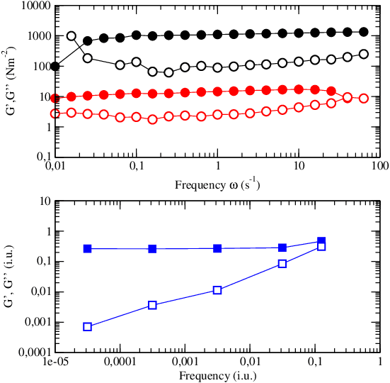
Figure 4: Top) Experimental measurements of the elastic modulus (filled symbols) and loss modulus (empty symbols) for two different biofilms: one grown under shaking conditions (black) and one under static conditions (red). Bottom) $G^{{}^{\prime}}$ (filled symbols) and $G^{{}^{\prime\prime}}$ (empty symbols) computed for the biofilm model. Data refer to $N_{b}=184$, $N_{p}=80$, $l=100$, $N_{s}=35000$ and 2000 cross-links.

By increasing the externally imposed stress (or frequency), we observed increasingly larger absolute values of the $G^{{}^{\prime\prime}}$, which become comparable to $G^{{}^{\prime}}$ for large frequencies (at least under static conditions, in red in Fig. 4), as one would expect in a viscoelastic material. In the biofilm grown under shaking conditions $G^{{}^{\prime\prime}}$ does not reach the same value of $G^{{}^{\prime}}$ for large frequencies (in black in Fig. 4). Due to the technical limitations of the used rheometer, we underline that we could not measure the stress moduli of the P. fluorescens biofilm grown under shaking conditions for frequencies beyond 100 Hz (Fig. 4, top panel, black symbols). However, we expect that eventually the trend of the stress response of the P. fluorescens biofilms developed under shaken conditions will behave similarly to the observed stress response of the biofilm developed under static conditions (Fig. 4, top panel).

The obtained values for the storage moduli (filled symbols) are always larger than the ones for the loss moduli (empty symbols), both in experiments and in simulations. This result is consistent with our already published workJara et al. (2021), where we showed that P. fluorescens biofilms grow better under shaking growth conditions than under static ones, the former leading to a higher bacterial density and a thicker biofilm matrix. Augmented aeration and nutrient concentration within the biofilm provides an optimal growth conditions for the bacteria that eventually leads to the production of a larger amount of cross-links within the EPS polymer matrix and produces a stiffer biofilm structure Jara et al. (2021).

According to the established experimental conditions, we numerically compute the shear moduli of the biofilm model by changing the stress frequency over 4 order of magnitudes (Fig. 4, bottom panel) . We assume that the main difference between the biofilm grown under static and shaking conditions is only in in the matrix composition, being the one of the shaken-grown biofilm richer in cross-links. In general terms, the numerical results (expressed in internal units, i.u.) exhibits the same overall trend (Fig. 4, top panel) observed for the P. fluorescens biofilms (both static and shaken). Overall, for all tested frequencies, $G^{{}^{\prime}}$ is larger than $G^{{}^{\prime\prime}}$ that remains almost constant. However, $G^{{}^{\prime\prime}}$ increases with increasing frequency and eventually converges with $G^{{}^{\prime}}$ at the highest simulated frequency. A qualitative difference is the drop in G” shown by simulations at low frequencies. A dominance of the flowing solvent is the halmark for these simulations at low frequency of shearing. This is not however observed in experiments (see Fig. 4; top panel), which a change of the number of cross-links $CL$, bacteria $N_{b}$, polymers $N_{p}$ or hydration level $N_{s}$ within the studied parameter space does not change the trend of our obtained computational results. A time-modulated solvent-matrix interaction could be introduced to correct this viscoelastic bias of simulations not found in experiments.

IV Discussion

Biofilms are composed of bacteria that secrete a network of extracellular polymeric substances (EPS) producing a viscoelastic matrix to which they eventually crosslink. Within a clinical or industrial environment, biofilm formation faces major issues. The mathematical modelling of complex biofilms might be of support, providing accurate descriptions and predictions that include physical parameters as hydrodynamics, solute mass transport or dynamics of the bacterial population within the biofilm. However, up-to-date modelling of biofilms, even at a coarse-grained level, has not been completely satisfactory. The parametrization of the individual components of a biofilm increases the complexity of the algorithm beyond computational capacity Calude and Longo (2017). Therefore, a simplification is needed that often leads to covering relevant experimental information.

In our work, we present a mesoscopic coarse grained dissipative particle dynamics (DPD) approach to model a mature bacterial biofilm. DPD models allow to simulate short range interactions of any particle and thus give a detailed picture of its close surroundings allowing an increase in spatial resolution. This is an important advantage over generally used long-range interaction modelsGroot (2004). Moreover the "soft" nature of DPD interactions allows to increase the integration time by few orders of magnitude, which permits to explore time scales normally inaccessible to atomistic simulations. Most importantly, our model explicitly includes hydrodynamics and thermal fluctuations, which are known to play an important role in biological systems such as biofilms Krsmanovic et al. (2021).

We generated a series of biofilm conformations by changing the composition, the number of bacteria, the number of polymers or varied the cross-linking and the hydration level of the biofilm. Next, the biofilm underwent deformations when exposed to an external oscillatory shear with different amplitudes and frequencies spanning 4 order of magnitudes. We computed the shear moduli and presented the model predictions for the different systems finding the computational results in agreement with experiments. When varying the number of bacteria, we observed that $G^{{}^{\prime}}$ remains constant throughout the $N_{b}$ range, in agreement with considering a biofilm as a polymer-colloid viscoelastic medium. The loss modulus $G^{{}^{\prime\prime}}$ increased linearly with $N_{b}$ reaching the values of the storage modulus for the largest number of bacteria. However, since $G^{{}^{\prime\prime}}$ is always smaller than $G^{{}^{\prime}}$, the biofilm system behaves as a pasty material, with a relative high structural rigidity $G^{{}^{\prime}}>G^{{}^{\prime\prime}}$. When increasing the number of entangled polymers, we observed that it was easier for the biofilm to generate a solid-like network with an increased rigidity. The out-phase stress response increases with increasing number of polymers. However, since the increase of $G^{{}^{\prime\prime}}$ is quite small when compared to the response caused by the presence of bacteria, we considered $G^{{}^{\prime\prime}}$ for polymer and solvent to be constant. Therefore, the present cross-linked matrix polymers might be entangeled, which allows expansion of the biofilm but at the same time provides rigidity. When studying the mechanical response of the system for different hydration levels, we observed that increasing the number of solvent particles, the biofilm was fully hydrated and the storage modulus decreased. The more the solvent, the softer the storage modulus.

We have chosen a set of parameter to compare our numerical data with rheological experiments performed on P. fluorescens biofilms grown under static and shaken conditions. We choose to study biofilms formed by P. fluorescens for two reasons. 1) It is the same model system we chose in our previous studyJara et al. (2021), and it will be easier for us to compare these results to the already published ones. 2)Although the model microorganism used in this work for experimental data is considered non-pathogenic, other members of the genus P. fluorescens such as Pseudomonas aeruginosa is an opportunistic pathogen that is frequently associated with chronic biofilm infections. Overall, the composition of the EPS is similar in both species, with a high proportion of acetylated polysaccharides (alginate-like) and extracellular DNA (Kives et al., 2006; Jennings et al., ) and therefore suggested to expose a similar mechanical behaviour. Knowledge on the timing of mechanical transitions within biofilms may guide future strategies that allow the penetration of antimicrobial agents into “soften” biofilm matrices.

By accurately comparing the experimental to the numerical results, we conclude that our proposed coarse grained model catches qualitatively the moduli behaviors over four order of magnitudes as observed in Fig 4. The measured elastic modulus is always higher in experiments and simulations than the loss modulus. Although $G^{{}^{\prime}}$ and $G^{{}^{\prime\prime}}$ tend to converge for high frequency, the simulations contain more viscous relaxation than reflected by experiments. Overall, the qualitative trends observed as soft solids for both studied biofilms (static and shaken) are recovered by our numerical findings, which could be eventually enhanced by including sticking details on the solvent-matrix interactions. Moreover, this concordance exhibits the potential of the use of a coarse graianed DPD approach when modelling complex biofilms. Even though the model strongly relies on an a priori detailed study of the parameter space, in future prospective, this will allow us to evaluate in more detail the biofilm transitions from a predominantly solid-like system to predominantly liquid-like system, through the interplay of the elastic and loss moduli upon changing the biofilm composition.

Conflicts of interest

There are no conflicts to declare.

References

- Peterson et al. (2015) B. W. Peterson, Y. He, Y. Ren, A. Zerdoum, M. R. Libera, P. K. Sharma, A.-J. van Winkelhoff, D. Neut, P. Stoodley, H. C. van der Mei, and H. J. Busscher, FEMS Microbiology Reviews 39, 234 (2015).
- Flemming and Wingender (2010) H. Flemming and J. Wingender, J. Nat Rev Microbiol 8, 623 (2010).
- Donlan (2001a) R. Donlan, J. Emerg. Infect. Dis. 7, 277 (2001a).
- Hoiby et al. (2010) N. Hoiby et al., Int J Antimicrobial Agents 35, 322 (2010).
- Khatoon et al. (2018) Z. Khatoon, C. D. McTiernan, E. J. Suuronen, T.-F. Mah, and E. I. Alarcon, Heliyon 4, e01067 (2018).
- Milchev and Binder (2013) A. Milchev and K. Binder, Macromolecules , 131031083721001 (2013).
- Duan et al. (2008) J. Duan, S. Wu, X. Zhang, G. Huang, M. Du, and B. Hou, Electrochimica Acta 54, 22 (2008).
- Mansour and Elshafei (2016) R. Mansour and A. Elshafei, British Biotechnology Journal 14, 1 (2016).
- Schultz and Swain (2000) M. P. Schultz and G. W. Swain, Biofouling 15, 129 (2000).
- Zhao et al. (2016) G. Zhao, Y. J. Yu, J. L. Yan, M. C. Ding, X. G. Zhao, and H. Y. Wang, Physical Review B 93, 140203 (2016).
- J.N.Wilking et al. (2011) J.N.Wilking, T.E.Angelini, A.Seminara, M.P.Brenner, and D.A.Weitz, MRS Bulletin 36, 385 (2011).
- Garrett et al. (2008) T. R. Garrett, M. Bhakoo, and Z. Zhang, Progress in natural science 18, 1049 (2008).
- Sveinbjörnsson et al. (2012) B. R. Sveinbjörnsson, R. A. Weitekamp, G. M. Miyake, and Y. Xia, Proceedings Of The National Academy Of Sciences Of The United States Of America 109, 14332 (2012).
- Klapper and Dockery (2010) I. Klapper and J. Dockery, SIAM Rev. 52, 221 (2010).
- Wang and Thanou (2010) M. Wang and M. Thanou, Pharmacological research : the official journal of the Italian Pharmacological Society 62, 90 (2010).
- Zhang et al. (2008) T. Zhang, N. G. Cogan, and Q. Wang, SIAM J. Appl. Math 69, 641 (2008).
- Kandemir et al. (2018) N. Kandemir, W. Vollmer, N. S. Jakubovics, and J. Chen, Scientific Reports 8, 10893 (2018).
- Picioreanu et al. (1999) C. Picioreanu, M. C. M. van Loosdrecht, and J. J. Heijnen, Water Sci. Technol. 39, 115 (1999).
- Picioreanu et al. (2004) C. Picioreanu, J. U. Kreft, and M. C. M. van Loosdrecht, Appl. Environ. Microbiol. 70, 3024 (2004).
- Horn and Lackner (2014) H. Horn and S. Lackner, Adv Biochem Eng Biotechnol 146, 53 (2014).
- Eberl et al. (2008) H. J. Eberl et al., Computing Intensive Simulations in Biofilm Modeling (22nd International Symposium on High Performance Computing Systems and Applications, 2008).
- Liu and Balazs (2018a) Y. Liu and A. C. Balazs, Langmuir 34, 1807 (2018a).
- Xu et al. (2011a) Z. Xu et al., Phys Rev E 83, 066702 (2011a).
- Bol et al. (2012) M. Bol et al., Critical Reviews in Biotechnology 33, 145 (2012).
- Hammond et al. (2014a) J. Hammond et al., Computer Modeling in Engineering and Sciences 98, 295 (2014a).
- Stotsky et al. (2016a) J. A. Stotsky et al., J. Comp. Phys. 317, 204 (2016a).
- Peskin (1977) C. Peskin, J. Comput.Phys. 81, 372 (1977).
- Peskin (2002) C. Peskin, Acta Numer. 11, 479 (2002).
- Hammond et al. (2014b) J. Hammond, E. Stewart, J. Younger, M. Solomon, and D. Bortz, Comput. Model. Eng. Sci. 98, 295 (2014b).
- Stotsky et al. (2016b) J. A. Stotsky, J. F. Hammond, L. Pavlovsky, E. J. Stewart, J. G. Younger, M. J. Solomon, and D. M. Bortz, J. Comput. Phys 317, 204 (2016b).
- Pavlovsky et al. (2013) L. Pavlovsky, J. G. Younger, and M. J. Solomon, Soft matter 9, 122 (2013).
- Stotsky et al. (2018) J. A. Stotsky, V. Dukic, and D. M. Bortz, Euro. Jnl of Applied Mathematics , 1 (2018).
- Barai et al. (2016) P. Barai, A. Kumar, and P. P. Mukherjee, PLoS One 11, e0165593 (2016).
- Xu et al. (2011b) Z. Xu, P. Meakin, A. Tartakovsky, and T. D. Scheibe, Physical Review E 83, 066702 (2011b).
- Mukhi and Vishwanathan (2021) M. Mukhi and A. Vishwanathan, Molecular Diversity , 1 (2021).
- Raos and Casalegno (2011) G. Raos and M. Casalegno, J. Chem. Phys. 134, 054902 (2011).
- Liu and Balazs (2018b) Y. Liu and A. C. Balazs, Langmuir 34, 1807 (2018b).
- Xu et al. (2011c) Z. Xu, P. Meakin, A. Tartakovsky, and T. D. Scheibe, Physical Review E 83, 066702 (2011c).
- Jara et al. (2021) J. Jara, F. Alarcon, A. K. Monnappa, J. I. Santos, V. Bianco, P. Nie, M. P. Ciamarra, A. Canales, L. Dinis, I. Lopez-Montero, C. Valeriani, and B. Orgaz, Frontiers in Microbiology 11, 588884 (2021).
- Guido et al. (2006) R. Guido, M. Margherita, and S. Elli, Macromolecules 39, 6744 (2006).
- Plimpton (1995) S. Plimpton, Journal of computational physics 117, 1 (1995).
- Hoogerbrugge and Koelman (1992) P. Hoogerbrugge and J. M. V. A. Koelman, EPL 19, 155 (1992).
- Groot and Warren (1997) R. D. Groot and P. B. Warren, The Journal of chemical physics 107, 4423 (1997).
- Donlan (2001b) R. M. Donlan, Emerging infectious diseases 7, 277 (2001b).
- Alonci et al. (2018) G. Alonci, F. Fiorini, P. Riva, F. Monroy, I. López-Montero, S. Perretta, and L. De Cola, ACS Applied Bio Materials 1, 1301 (2018).
- Richardson and Te Whaiti (1978) B. C. Richardson and I. E. Te Whaiti, New Zealand Journal of Dairy Science and Technology 13, 172 (1978).
- Calude and Longo (2017) C. S. Calude and G. Longo, Foundations of science 22, 595 (2017).
- Groot (2004) R. D. Groot, in Novel Methods in Soft Matter Simulations (Springer, 2004) pp. 5–38.
- Krsmanovic et al. (2021) M. Krsmanovic, D. Biswas, H. Ali, A. Kumar, R. Ghosh, and A. K. Dickerson, Advances in Colloid and Interface Science 288, 102336 (2021).
- Kives et al. (2006) J. Kives, B. Orgaz, and C. Sanjosé, Colloids Surf B Biointerfaces 52, 123 (2006).
- (51) L. K. Jennings, K. M. Storek, H. E. Ledvina, C. Coulon, L. S. Marmont, I. Sadovskaya, P. R. Secor, B. S. Tseng, M. Scian, A. Filloux, D. J. Wozniak, P. L. Howell, and M. R. Parsek, Proceedings of the National Academy of Sciences 112, 11353.