Quantum–classical correspondence in spin–boson equilibrium states
at arbitrary coupling

Abstract

The equilibrium properties of nanoscale systems can deviate significantly from standard thermodynamics due to their coupling to an environment. For the generalised $\theta$-angled spin-boson model, we first derive a compact and general form of the classical equilibrium state including environmental corrections to all orders. Secondly, for the quantum spin-boson model we prove, by carefully taking a large spin limit, that Bohr’s quantum-classical correspondence persists at all coupling strengths. This correspondence gives insight into the conditions for a coupled quantum spin to be well-approximated by a coupled classical spin-vector. Thirdly, we demonstrate that previously identified environment-induced ‘coherences’ in the equilibrium state of weakly coupled quantum spins, do not disappear in the classical case. Finally, we provide the first classification of the coupling parameter regimes for the spin-boson model, from weak to ultrastrong, both for the quantum case and the classical setting. Our results shed light on the interplay of quantum and mean force corrections in equilibrium states of the spin-boson model, and will help draw the quantum to classical boundary in a range of fields, such as magnetism and exciton dynamics.

Bohr’s correspondence principle [1] played an essential role in the early development of quantum mechanics. Since then, a variety of interpretations and applications of the correspondence principle have been explored [2, 3, 4, 5, 6, 7, 8, 9]. One form asks if the statistical properties of a quantum system approach those of its classical counterpart in the limit of large quantum numbers [4, 5]. This question was answered affirmatively by Millard and Leff, and Lieb for a quantum spin system [2, 3]. They proved that the system’s thermodynamic partition function $Z_{\mathrm{S}}^{\mathrm{qu}}$ associated with the Gibbs state, converges to the corresponding classical partition function $Z_{\mathrm{S}}^{\mathrm{cl}}$, in the limit of large spins. Such correspondence gives insight into the conditions for a quantum thermodynamic system to be well-approximated by its classical counterpart [8, 9]. While $Z_{\mathrm{S}}^{\mathrm{qu}}$ is computationally tough to evaluate for many systems, $Z_{\mathrm{S}}^{\mathrm{cl}}$ offers tractable expressions with which thermodynamic properties, such as free energies, susceptibilities and correlation functions, can readily be computed [2, 3]. Similarly, many dynamical approaches solve a classical problem rather than the much harder quantum problem. For example, sophisticated atomistic simulations of the magnetisation dynamics in magnetic materials [10, 11, 12, 13, 14] solve the evolution of millions of interacting classical spins. A corresponding quantum simulation [15] would require no less than a full–blown quantum computer as its hardware.

Meanwhile, in the field of quantum thermodynamics, extensive progress has recently been made in constructing a comprehensive framework of “strong coupling thermodynamics” for classical [16, 17, 18, 19, 20, 21] and quantum [22, 23, 24, 25, 26, 27, 28, 29, 30, 31, 32] systems. This framework extends standard thermodynamic relations to systems whose coupling to a thermal environment can not be neglected. The equilibrium state is then no longer the quantum or classical Gibbs state, but must be replaced with the environment-corrected mean force (Gibbs) state [33, 31, 32]. These modifications bring into question the validity of the correspondence principle when the environment-coupling is no longer negligible. Mathematically, the challenge is that in addition to tracing over the system, one must also evaluate the trace over the environment.

Strong coupling contributions are present for both classical and quantum systems. However, a quantitative characterisation of the difference between these two predictions, in various coupling regimes, is missing. For example, apart from temperature, what are the parameters controlling the deviations between the quantum and classical spin expectation values? Do coherences, found to persist in the mean force equilibrium state of a quantum system [34], decohere when taking the classical limit? How strong does the environmental coupling need to be for the spin-boson model to be well-described by weak or ultrastrong coupling approximations? In this paper, we answer these questions for the particular case of a spin $S_{0}$ coupled to a one-dimensional bosonic environment such that both dephasing and detuning can occur ($\theta$-angled spin-boson model).

Setting. This generalised version of the spin-boson model [35, 36] describes a vast range of physical contexts, including excitation energy transfer processes in molecular aggregates described by the Frenkel exciton Hamiltonian [37, 38, 39, 40, 41, 42, 43], the electronic occupation of a double quantum dot whose electronic dipole moment couples to the substrate phonons in a semi-conductor [34], an electronic, nuclear or effective spin exposed to a magnetic field and interacting with an (anisotropic) phononic, electronic or magnonic environment [44, 54, 55, 56, 57], and a plethora of other aspects of quantum dots, ultracold atomic impurities, and superconducting circuits [45, 46, 47, 48]. In all these contexts, an effective “spin” $\mathbf{S}$ interacts with an environment, where $\mathbf{S}$ is a vector of operators (with units of angular momentum) whose components fulfil the angular momentum commutation relations $[S_{j},S_{k}]=i\hbar\sum_{l}\epsilon_{jkl}S_{l}$ with $j,k,l=x,y,z$. We will consider spins of any length $S_{0}$, i.e. $\mathbf{S}^{2}=S_{0}(S_{0}+\hbar)\boldsymbol{1}$. The system Hamiltonian is

$$H_{\mathrm{S}}=-\omega_{\mathrm{L}}S_{z},$$ (1)

where the system energy level spacing is $\hbar\omega_{\mathrm{L}}>0$ and the energy axis is in the $-z$-direction without loss of generality. For a double quantum dot, the frequency $\omega_{\mathrm{L}}$ is determined by the energetic detuning and the tunneling between the dots [34]. For an electron spin with $S_{0}=\hbar/2$, the energy gap is set by a (negative) gyromagnetic ratio $\gamma$ and an external magnetic field $\mathbf{B_{\mathrm{ext}}}=-B_{\mathrm{ext}}\mathbf{\hat{z}}$, such that $\omega_{\mathrm{L}}=\gamma B_{\mathrm{ext}}$ is the Larmor frequency.

The spin system is in contact with a bosonic reservoir, which is responsible for the dissipation and equilibration of the system. Typically, this environment will consist of phononic modes or an electromagnetic field [49, 32]. The bare Hamiltonian of the reservoir is

$$H_{\mathrm{R}}=\frac{1}{2}\int_{0}^{\infty}\mathrm{d}\omega\,\left(P_{\omega}^{2}+\omega^{2}X_{\omega}^{2}\right),$$ (2)

where $X_{\omega}$ and $P_{\omega}$ are the position and momentum operators of the reservoir mode at frequency $\omega$ which satisfy the canonical commutation relations $[X_{\omega},P_{\omega^{\prime}}]=i\hbar\,\delta(\omega-\omega^{\prime})$. With the identifications made in (1) and (2), the system-reservoir Hamiltonian is

$$H_{\mathrm{tot}}=H_{\mathrm{S}}+H_{\mathrm{R}}+H_{\mathrm{int}},$$ (3)

which contains a system-reservoir coupling $H_{\mathrm{int}}$. Physically, the coupling can often be approximated to be linear in the canonical reservoir operators [32], and is then modelled as [50, 49, 34]

$$H_{\mathrm{int}}=S_{\theta}\int_{0}^{\infty}\mathrm{d}\omega\,C_{\omega}X_{\omega},$$ (4)

where the coupling function $C_{\omega}$ determines the interaction strength between the system and each reservoir mode $\omega$. $C_{\omega}$ is related to the reservoir spectral density $J_{\omega}$ via $J_{\omega}=C_{\omega}^{2}/(2\omega)$. It is important to note that the coupling is to the spin (component) operator $S_{\theta}=S_{z}\cos\theta-S_{x}\sin\theta$ which is at an angle $\theta$ with respect to system’s bare energy axis, see Fig. 1. For example, for a double quantum dot [34], the angle $\theta$ is determined by the ratio of detuning and tunnelling parameters.

In what follows we will need an integrated form of the spectral density, namely

$$Q=\int_{0}^{\infty}\mathrm{d}\omega\,\frac{J_{\omega}}{\omega}=\int_{0}^{\infty}\mathrm{d}\omega\,\frac{C_{\omega}^{2}}{2\omega^{2}}.$$ (5)

This quantity is a measure of the strength of the system–environment coupling and it is sometimes called “reorganization energy” [51, 52, 53, 33]. The analytical results discussed below are valid for arbitrary coupling functions $C_{\omega}$ (or reorganisation energies $Q$). The plots assume Lorentzians $J_{\omega}=(2\Gamma\,Q/\pi)\,\omega_{0}^{2}\omega/((\omega_{0}^{2}-\omega^{2})^{2}+\Gamma^{2}\omega^{2})$, where $\omega_{0}$ is the resonant frequency of the Lorentzian [44] and $\Gamma$ the peak width.

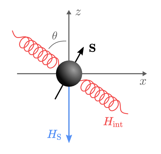
Figure 1: Illustration of bare and interaction energy axes. A spin operator (vector) $\mathbf{S}$ with system Hamiltonian $H_{\mathrm{S}}$ with energy axis in the $-z$-direction is coupled in $\theta$-direction to a harmonic environment via $H_{\mathrm{int}}$.

We will model $H_{\mathrm{tot}}$ (Eq. (3)) either fully quantum mechanically as detailed above, or fully classically. To obtain the classical case, the spin $\mathbf{S}$ operator will be replaced by a three-dimensional vector of length $S_{0}$, and the reservoir operators $X_{\omega}$ and $P_{\omega}$ will be replaced by classical phase–space coordinates. Below, we evaluate the spin’s so-called mean force (Gibbs) states, CMF and QMF, for the classical and quantum case, respectively. The mean force approach postulates [32] that the equilibrium state of a system in contact with a reservoir at temperature $T$ is the mean force (MF) state, defined as

$$\tau_{\mathrm{MF}}:=\operatorname{tr}_{\mathrm{R}}[\tau_{\mathrm{tot}}]=\operatorname{tr}_{\mathrm{R}}\left[\frac{e^{-\beta H_{\mathrm{tot}}}}{Z_{\mathrm{tot}}}\right].$$ (6)

That is, $\tau_{\mathrm{MF}}$ is the reduced system state of the global Gibbs state $\tau_{\mathrm{tot}}$, where $\beta=1/k_{\mathrm{B}}{}T$ is the inverse temperature with $k_{\mathrm{B}}$ the Boltzmann constant, and $Z_{\mathrm{tot}}$ is the global partition function. Quantum mechanically, $\operatorname{tr}_{\mathrm{R}}$ stands for the operator trace over the reservoir space while classically, “tracing” is done by integrating over the reservoir degrees of freedom. Further detail on classical and quantum tracing for the spin and the reservoir, respectively, is given in Appendix A.

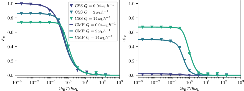
Figure 2: Classical mean force and steady–state spin expectation values. Normalised expectation values of the classical spin components $s_{z}$ (left) and $s_{x}$ (right) as a function of temperature. These are obtained with: (css) the long time average of the dynamical evolution of the spin, $s_{k}=\langle S_{k}\rangle_{\mathrm{\textsc{css}}}/S_{0}$; and (CMF) the classical MF state (Eq. (7)), $s_{k}=\langle S_{k}\rangle_{\mathrm{MF}}/S_{0}$. These are shown for three different coupling strengths $Q=0.04\,\omega_{\mathrm{L}}\hbar^{-1},2\,\omega_{\mathrm{L}}\hbar^{-1},14\,\omega_{\mathrm{L}}\hbar^{-1}$, that range from the weak to the strong coupling regimes. In all three cases, we see that the MF predictions are fully consistent with the results of the dynamics. All plots are for Lorentzian coupling with $\omega_{0}=7\omega_{\mathrm{L}}$, $\Gamma=5\omega_{\mathrm{L}}$, and coupling angle $\theta=45^{\circ}$. The temperature scale shown corresponds to a spin $S_{0}=\hbar/2$.

While the formal definition of $\tau_{\mathrm{MF}}$ is deceptively simple, carrying out the trace over the reservoir – to obtain a quantum expression of $\tau_{\mathrm{MF}}$ in terms of system operators alone – is notoriously difficult. Often, expansions for weak coupling are made [22, 34]. For a general quantum system (i.e. not necessarily a spin), an expression of $\tau_{\mathrm{MF}}$ has recently been derived in this limit [33]. Furthermore, recent progress has been made on expressions of the quantum $\tau_{\mathrm{MF}}$ in the limit of ultrastrong coupling [33], and for large but finite coupling [31, 32, 58]. Moreover, high temperature expansions have been derived that are also valid at intermediate coupling strengths [43]. However, the low and intermediate temperature form of the quantum $\tau_{\mathrm{MF}}$ for intermediate coupling is not known, neither in general nor for the $\theta$–angled spin boson model [59].

Classical MF state at arbitrary coupling. In contrast, here we establish that the analogous problem of a classical spin vector of arbitrary length $S_{0}$, coupled to a harmonic reservoir via Eq. (4), is tractable for arbitrary coupling function $C_{\omega}$ and arbitrary temperature. By carrying out the (classical) partial trace over the reservoir, i.e. $\operatorname{tr}_{\mathrm{R}}^{\mathrm{cl}}[\tau_{\mathrm{tot}}]$, we uncover a rather compact expression for the spin’s CMF state $\tau_{\mathrm{MF}}$ and the CMF partition function $\tilde{Z}_{\mathrm{S}}^{\mathrm{cl}}$:

$$\tau_{\mathrm{MF}} =\frac{e^{-\beta(H_{\mathrm{S}}-QS_{\theta}^{2})}}{\tilde{Z}_{\mathrm{S}}^{\mathrm{cl}}}$$ (7)

$$\text{with}\quad\tilde{Z}_{\mathrm{S}}^{\mathrm{cl}} =\operatorname{tr}_{\mathrm{S}}^{\mathrm{cl}}[e^{-\beta(H_{\mathrm{S}}-QS_{\theta}^{2})}].$$

The state $\tau_{\mathrm{MF}}$ clearly differs from the standard Gibbs state by the presence of the reorganisation energy term $-QS_{\theta}^{2}$. The quadratic dependence on $S_{\theta}$ changes the character of the distribution, from a standard exponential to an exponential with a positive quadratic term, altering significantly the state whenever the system–reservoir coupling is non-negligible.

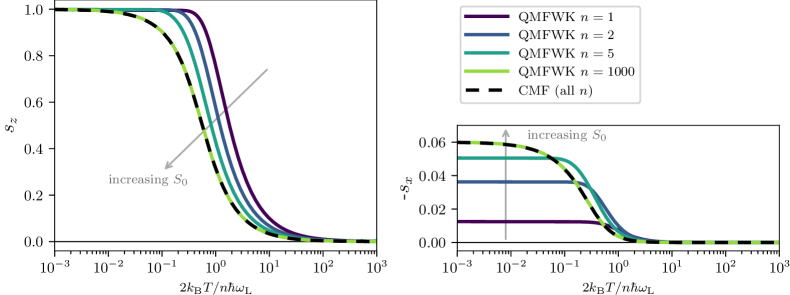
Figure 3: Classical and quantum mean force spin components. Normalised expectation values of the spin components $s_{z}$ (left) and $s_{x}$ (right) obtained with: (QMFWK) the quantum MF partition function $\tilde{Z}_{\mathrm{S}}^{\mathrm{qu}}$ in the weak coupling limit for a spin of length $S_{0}=n\hbar/2$ ($n=1,2,5,100$); (CMF) the classical MF partition function $\tilde{Z}_{\mathrm{S}}^{\mathrm{cl}}$ given in (7). As the length $S_{0}$ of the quantum spin is increased, the quantum mean force prediction QMFWK converges to that corresponding to the CMF state. Non-zero $s_{x}$ (right) indicate “coherences” with respect to the system’s bare energy axis ($z$). These arise entirely due to the spin-reservoir interaction. Such coherences have been discussed for the quantum case [34]. Here we find that they also arise in the classical CMF and, comparing like with like for the same spin length $S_{0}=\hbar/2$, the classical “coherences” are larger than those of the quantum spin. All plots are for a weak coupling strength, $\alpha=0.06$, and $\theta=\pi/4$.

Throughout this article, we will consider that the MF state is the equilibrium state reached by a system in contact with a thermal bath. While this is widely thought to be the case, some open questions remain about formal proofs showing the convergence of the dynamics towards the steady state predicted by the MF state [32, 25, 26, 27, 34, 60, 61, 62, 63, 64, 65]. For example, for quantum systems, this convergence has only been proven in the weak [22] and ultrastrong limits [31], while for intermediate coupling strengths there is numerical evidence for the validity of the MF state [36]. Here, we numerically verify the convergence of the dynamics towards the MF state for the case of the classical spin at arbitrary coupling strength. This is possible thanks to the numerical method proposed in [44]. Fig. 2 shows the long time average of the spin components once the dynamics has reached steady state (css, triangles), together with the expectation values predicted by the static MF state (CMF, solid lines), for a wide range of coupling strengths going from weak to strong coupling . We find that both predictions are in excellent agreement, providing strong evidence for the convergence of the dynamics towards the MF. The compact expression (7) for the CMF state, as well as the numerical verification that the dynamical steady state matches it, are the first result of this paper.

Quantum–classical correspondence. We now demonstrate that the quantum partition function $\tilde{Z}_{\text{S}}^{\text{qu}}$, which includes arbitrarily large mean force corrections, converges to the classical one, $\tilde{Z}_{\text{S}}^{\text{cl}}$ in Eq. (7).

A well-known classical limit of a quantum spin is to increase the quantum spin’s length, $S_{0}\to\infty$. This is because, when $S_{0}$ increases, the quantised angular momentum level spacing relative to $S_{0}$ decreases, approaching a continuum of states that can be described in terms of a classical vector [1]. Taking the large spin limit for a spin-$S_{0}$ system can be achieved following an approach used by Fisher when treating an uncoupled spin with Hamiltonian $H_{\mathrm{S}}$ [67]. This involves introducing a rescaling of the spin operators via $s_{j}=S_{j}/S_{0}$ so that the commutation rule becomes $[s_{j},s_{k}]=i\hbar\,\epsilon_{jkl}\,s_{l}/S_{0}$. Hence, in the limit of $S_{0}\to\infty$, the scaled operators will commute, so in that regard they can be considered as classical quantities [67]. Millard & Leff  [2] take this further and prove, for any spin Hamiltonian $H$ in the spin Hilbert space ${\cal H}_{S}$, the identity

$$\lim_{S_{0}\to\infty}\frac{\hbar}{2S_{0}+\hbar}\,\operatorname{tr}_{\mathrm{S}}^{\mathrm{qu}}\left[e^{-\beta H}\right]$$

$$= \lim_{S_{0}\to\infty}\frac{1}{4\pi}\int_{0}^{2\pi}d\varphi\int_{0}^{\pi}d\vartheta\sin\vartheta\,e^{-\beta H(S_{0},\vartheta,\varphi)},$$ (8)

provided the limit on the right hand side exists . Here $H(S_{0},\vartheta,\varphi)$ is the classical spin-$S_{0}$ Hamiltonian, where the spin-vector $\mathbf{S}$ is parametrised by two angles, $\varphi$ and $\vartheta$, such that $s_{x}=S_{0}\sin\vartheta\cos\varphi,s_{y}=S_{0}\sin\vartheta\sin\varphi$ and $s_{z}=S_{0}\cos\vartheta$. Eq. (Quantum–classical correspondence in spin–boson equilibrium states at arbitrary coupling) was further confirmed by Lieb who provides a rigorous argument based on the properties of spin-coherent states [3].

Note, though, if one simply takes the $S_{0}\to\infty$ limit in (Quantum–classical correspondence in spin–boson equilibrium states at arbitrary coupling), with $H$ being the system Hamiltonian $H_{S}\propto S_{0}$, that would have the same effect as sending $\beta\to\infty$; namely, all population will go to the ground state. Instead, to maintain a non-trivial temperature dependence after taking the $S_{0}$-limit requires a further rescaling step. One approach involves a rescaling of the physical parameters of the Hamiltonian $H$, as followed, e.g., by Fisher [67]. A second approach is to rescale the inverse temperature via $\beta S_{0}=\beta^{\prime}$, and take the limit $S_{0}\to\infty$ with $\beta^{\prime}$ held fixed. This is the limit we will take here. The effect of this constrained limit can readily be seen for the thermal states of the uncoupled classical or quantum spin. The classical partition function $Z_{\mathrm{S}}^{\mathrm{cl}}(\beta S_{0})={\sinh(\beta S_{0}\omega_{\mathrm{L}})/\beta S_{0}\omega_{\mathrm{L}}}$ is left invariant because $\beta$ and $S_{0}$ always appear together in $Z_{\mathrm{S}}^{\mathrm{cl}}$. In contrast, the quantum partition function $Z_{\mathrm{S}}^{\mathrm{qu}}(\beta,S_{0})=\sinh(\beta(S_{0}+\hbar/2)\omega_{\mathrm{L}})/\sinh(\beta\hbar\omega_{\mathrm{L}}/2)$ is altered in the constrained limit, since $Z_{\mathrm{S}}^{\mathrm{qu}}$ separately depends on $\beta$ and $S_{0}$. Eq. (Quantum–classical correspondence in spin–boson equilibrium states at arbitrary coupling) then expresses the convergence of the partition functions [67, 2, 3], i.e. $\frac{\hbar}{2S_{0}+\hbar}\,Z_{\mathrm{S}}^{\mathrm{qu}}(\beta,S_{0})\to Z_{\mathrm{S}}^{\mathrm{cl}}(\beta S_{0})$.

We now take a step further and extend this result to the case of a spin coupled to a reservoir. The first step is to consider that the relevant Hilbert space is now the tensor product space of spin and reservoir degrees of freedom, ${\cal H}_{S}\otimes{\cal H}_{B}$. It was argued by Lieb [3] that (Quantum–classical correspondence in spin–boson equilibrium states at arbitrary coupling) remains valid in this case, i.e. even when $H\in{\cal H}_{S}\otimes{\cal H}_{B}$. This means we can replace $H$ in (Quantum–classical correspondence in spin–boson equilibrium states at arbitrary coupling) by our $H_{\mathrm{tot}}$. But note that the trace is still only over the system Hilbert space ${\cal H}_{S}$. Thus, formally one obtains an operator valued identity for operators on ${\cal H}_{B}$. The second step is then to evaluate the trace over the reservoir degrees of freedom. To do so, we start by writing the total unnormalised Gibbs state as

$$e^{-\beta H_{\mathrm{tot}}}=$$ (9)

$$\exp\left[-\beta^{\prime}\left(-\omega_{\mathrm{L}}s_{z}+\frac{H_{\mathrm{R}}}{S_{0}}+s_{\theta}\int_{0}^{\infty}\mathrm{d}\omega\,C_{\omega}X_{\omega}\right)\right].$$

with the rescaled inverse temperature $\beta^{\prime}=\beta S_{0}$. Since $\beta^{\prime}$ is constant as the limit $S_{0}\to\infty$ is taken, doing so rescales the spin operators, as required. But it also rescales $H_{\mathrm{R}}$ to $h_{\mathrm{R}}=H_{\mathrm{R}}/S_{0}$, which can be expressed in terms of rescaled reservoir operators, $p_{\omega}$ and $x_{\omega}$ where $p_{\omega}=P_{\omega}/\sqrt{S_{0}}$ and $x_{\omega}=X_{\omega}/\sqrt{S_{0}}$. The commutation relations are then $\left[x_{\omega},p_{\omega^{\prime}}\right]=i\hbar\,\delta(\omega-\omega^{\prime})/S_{0}$, so in the limit of $S_{0}\to\infty$, these two operators commute [69]. Thus, the classical limit of the spin induces a limit for the reservoir. I.e., the quantum nature of the reservoir is inevitably stripped away, so that the result eventually obtained is that of a classical spin coupled to a classical reservoir.

Written in terms of these rescaled reservoir operators, one now has

$$e^{-\beta H_{\mathrm{tot}}}=$$ (10)

$$\exp\left[-\beta^{\prime}\left(-\omega_{\mathrm{L}}s_{z}+h_{R}+s_{\theta}\int_{0}^{\infty}\mathrm{d}\omega\,C_{\omega}\sqrt{S_{0}}\,x_{\omega}\right)\right].$$

If one were to naively take the $S_{0}$-limit, then the interaction term dominates and the dependence on the bare system energy $-\omega_{\mathrm{L}}s_{z}$ drops out. To maintain a non-trivial dependence on both, bare and interaction energies, one needs to make an assumption on the scaling of the coupling function $C_{\omega}$ with spin-length $S_{0}$. We choose to keep the relative energy scales of the bare and interaction Hamiltonians the same throughout the $S_{0}$ limit. Eq. (10) shows that this requires a scaling of $C_{\omega}\propto 1/\sqrt{S_{0}}$. This implies a reorgansiation energy (5) scaling of

$$Q=\alpha\frac{\omega_{\mathrm{L}}}{S_{0}},$$ (11)

where $\alpha$ is a unit-free constant independent of $S_{0}$ and $\beta$. Inserted in the classical MF state (7) this shows that both, the system energy $H_{\mathrm{S}}$ as well as the correction that comes from the reservoir interaction, scale as $S_{0}$. The combined scaling of $Q$ with $S_{0}$ (Eq. (11)), and the rescaling of the inverse temperature, $\beta S_{0}=\beta^{\prime}=\mathrm{const}$, then leaves the CMF state (7) invariant under variation of $S_{0}$.

Crucially, given the same scaling, the QMF state defined by Eq. (6) will not be invariant under variation of $S_{0}$. Returning to the unnormalised total Gibbs state (10), taking the quantum trace over the spin, and using Eq. (Quantum–classical correspondence in spin–boson equilibrium states at arbitrary coupling), one obtains an identity that still contains the bath operators in contrast to the uncoupled spin. Finally taking the quantum trace over the reservoir on both sides, one finds

$$\lim_{S_{0}\to\infty}\frac{\hbar}{2S_{0}+\hbar}\frac{Z_{\mathrm{SR}}^{\mathrm{qu}}(\beta,S_{0},\alpha)}{Z_{\mathrm{R}}^{\mathrm{qu}}(\beta)}$$

$$= \lim_{S_{0}\to\infty}\frac{\hbar}{2S_{0}+\hbar}\tilde{Z}_{\mathrm{S}}^{\mathrm{qu}}(\beta,S_{0},\alpha)=\tilde{Z}_{\mathrm{S}}^{\mathrm{cl}}(\beta S_{0},\alpha).\quad$$ (12)

Here it was used that the fraction of the total quantum partition function divided by the bare quantum reservoir partition function is the quantum mean force partition function (see Appendix D) [70, 71]. In contrast to the quantum-classical correspondence established by Millard & Leff, and Lieb, for the standard Gibbs state partition functions, there now is a dependence on the spin-environment coupling strength $\alpha$. For the classical case, one has $\tilde{Z}_{\mathrm{S}}^{\mathrm{cl}}(\beta S_{0},\alpha)=\operatorname{tr}_{\mathrm{S}}^{\mathrm{cl}}[e^{-\beta S_{0}(H_{\mathrm{S}}/S_{0}-\alpha\,\omega_{\mathrm{L}}S_{\theta}^{2}/S_{0}^{2})}]$.

While we derived Eq. (12) assuming a constant ratio between bare and interaction energy, i.e. $C_{\omega}\propto 1/\sqrt{S_{0}}$, the quantum-classical correspondence also holds for other scalings. Indeed, when $C_{\omega}\propto 1/\sqrt{S_{0}^{p}}$ with $p>1$ the bare energy will grow much more rapidly than the interaction term in the limit $S_{0}\to\infty$. This immediately leads to the ultraweak coupling limit where the known quantum-classical correspondence (Quantum–classical correspondence in spin–boson equilibrium states at arbitrary coupling) applies. On the other hand, when $C_{\omega}\propto 1/\sqrt{S_{0}^{p}}$ with $0\leq p<1$, the interaction term will grow much more rapidly than the bare energy. As we show in Appendix G, in this ultrastrong limit [33], the quantum and classical mean force partition functions turn out to be identical. In this ultrastrong limit, the partition function loses all dependence on the coupling strength $\alpha$. Thus, while (12) is valid for $p>1$ and $0\leq p<1$, these scalings give a trivial correspondence, independent of $\alpha$. Only for the scaling (11) is a dependence of the mean force partition functions on the coupling strength retained.

The results presented here show the quantum-classical correspondence of the equilibrium states of the spin-boson model for the first time. The proof of this correspondence, valid at all coupling strengths, is the second result of the paper.

We remark that, in the above proof, it was assumed that $\alpha$ is independent of $\beta$. Physically this is not entirely accurate because the coupling $C_{\omega}$ is usually a function of temperature [72], albeit often a rather weak one. For the same limiting process to apply, a weak dependence on $\beta$ would need to be compensated by an equally weak additional dependence of $Q$ on $S_{0}$.

To visually illustrate the quantum to classical convergence, we choose a weak coupling strength, $\alpha=0.06$, for which an analytical form of the quantum $\tilde{Z}_{\mathrm{S}}^{\mathrm{qu}}$ is known [33]. Mean force spin component expectation values $s_{k}\equiv\langle S_{k}\rangle_{\mathrm{MF}}/S_{0}$ for $k=x,z$ can then readily be computed from the partition functions $\tilde{Z}_{\mathrm{S}}^{\mathrm{qu}}$ and $\tilde{Z}_{\mathrm{S}}^{\mathrm{cl}}$, respectively. Fig. 3 shows $s_{z}$ and $s_{x}$ for various spin lengths, $S_{0}=n\hbar/2$ with $n=1,2,5,1000$ for the quantum case (QMFWK, purple to green) and the classical case (CMF, dashed black). Note, that the $x$-axis is a correspondingly rescaled temperature, $2k_{\mathrm{B}}{}T/n\hbar\omega_{\mathrm{L}}$, a scaling under which the CMF remains invariant. The numerical results illustrate that the quantum $s_{z}$ and $s_{x}$ change with spin length $S_{0}=n\hbar/2$, and indeed converge to the classical prediction in the large spin limit, $n\to\infty$.

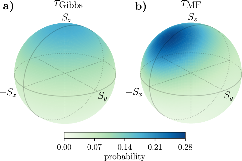
Figure 4: Coherences and inhomogeneous probabilities. Spin vector probability distributions (blue = high probability, white = low probability) as a function of three spin components on a sphere of radius $S_{0}$. a) The classical Gibbs state $\tau_{\mathrm{Gibbs}}$ is a homogeneous function of $H_{\mathrm{S}}$, i.e. it is constant over the energy shells of $H_{\mathrm{S}}$ which are fixed by the value of $S_{z}$. b) The classical mean force probability distribution $\tau_{\mathrm{MF}}$ given in (7), peaks in a direction with positive components in $-S_{x}$ and $S_{z}$ directions. This makes $\tau_{\mathrm{MF}}$ an inhomogeneous probability distribution over the energy shells of $H_{\mathrm{S}}$. Parameters for the plots: $\theta=\pi/4$, $k_{\mathrm{B}}{}T=S_{0}\omega_{\mathrm{L}}$, and $Q=\omega_{\mathrm{L}}/S_{0}$.

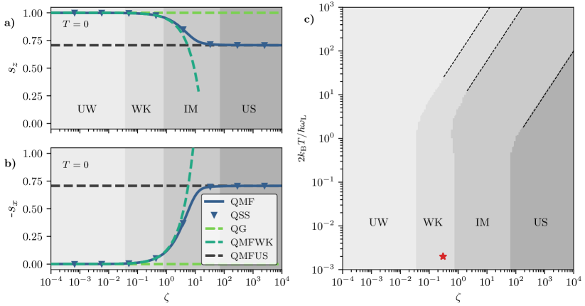
Figure 5: Quantum coupling regimes at $T=0$ K and $T>0$ K. Panels a) and b): Spin expectation values $s_{z}$ and $-s_{x}$ for the MF state (6) at $T=0$ for the total Hamiltonian (3) with $S_{0}=\hbar/2$, $\theta=\pi/4$ and different coupling strengths as quantified by the dimensionless parameter $\zeta$, see (13). We identify four coupling regimes for the numerically exact QMF state (solid dark blue):  Ultraweak coupling (UW), where the spin expectation values are consistent with the Gibbs state (QG, dashed light green);  Weak coupling (WK), where the expectation values are well approximated by a second order expansion in $\zeta$ (QMFWK, dashed turquoise) [34];  Ultrastrong coupling (US), where the asymptotic limit of infinitely strong coupling $\zeta\to\infty$ is valid (QMFUS, dashed grey) [33],  and Intermediate coupling (IM) where the QMF state is not approximated by any known analytical expression. The dynamical steady state of the quantum spin (QSS, dark blue triangles) is also computed using the reaction coordinate technique [73, 74, 75, 76]. Excellent agreement between the QSS and the QMF prediction is seen for all $\zeta$. Panel c): Coupling regimes as a function of temperature $T$ and coupling strength $\zeta$. With increasing temperature, the boundaries shift towards higher coupling $\zeta$. At large temperatures, all three boundaries follow a linear relation $T\propto\zeta$ (dashed lines).

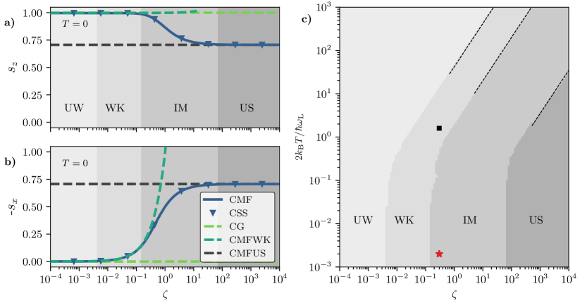
Figure 6: Classical coupling regimes at $T=0$ K and $T>0$ K. Same plot as Fig. 5, but here for the equilibrium state of a classical spin vector $\mathbf{S}$ with Hamiltonian Eq. (3). A particular $(T,\zeta)$-pair (red star) is identified for which the classical spin falls in the intermediate regime. For the same parameter pair, the quantum spin falls in the weak coupling regime, see red star in Fig. 5c). Moving the classical red star upwards in temperature until it reaches a point (black square) in the weak coupling regime that is laterally distanced from the boundaries similar to the quantum star, Fig. 5c), gives an effective temperature shift of $\Delta T=1.6\cdot 2\hbar\omega_{\mathrm{L}}/k_{\mathrm{B}}$. This example evidences significant differences between the environmental impact on quantum and classical equilibrium states.

Coherences. As seen in Fig. 3 (right panel), the $s_{x}$ spin-component in the quantum mean force state (solid purple line for spin-1/2) is non-zero at low temperatures, despite the fact that the bare system energy scale is set along the $z$-direction, see (1). Such non-zero $s_{x}$ implies the presence of energetic “coherences” in the system’s equilibrium state, as recently discussed in [77, 34] for a quantum spin-1/2. Considering the quantum–classical correspondence discussed above, a natural question is whether in the classical limit one can observe “decoherence”, in the sense of vanishing coherences. However, comparing like with like, we see in Fig. 3 that “coherences” are also present for a classical spin with length $S_{0}=\hbar/2$ (dashed black). Indeed, maybe surprisingly, classical “coherences” can be even larger in magnitude than those of a quantum spin with corresponding length $S_{0}$.

This observation reveals that the mechanism that gives rise to these coherences is not an intrinsically quantum one. Indeed, when we plot our CMF state (7) in Fig. 4b), one can immediately see that the classical spin alignment in equilibrium tilts towards the $-x$ direction compared to the Gibbs state shown in Fig. 4a). Such ‘inhomogenity’ of a classical distribution has recently been identified by A. Smith, K. Sinha, C. Jarzynski [78] as the classical analogue to quantum coherences in the context of thermodynamic work extraction [79, 80]. Here we uncover that the mechanism of producing such classical coherences can be due to the nature of the environmental coupling, which is asymmetric with respect to the bare Hamiltonian, see Fig. 1. This third finding, that coherences can be present even in classical equilibrium states, will have implications on a variety of fields, including quantum thermodynamics and quantum biology, which have so far interpreted a non-zero value of $s_{x}$ as a ‘quantum signature’.

Coupling regimes. Finally, we now classify the interaction strength necessary for the spin-boson model to fall in various coupling regimes, from ultra-weak to ultra-strong. To quantify the relative strength of coupling we use the dimensionless parameter

$$\zeta=\frac{QS_{0}}{\omega_{\mathrm{L}}},$$ (13)

which is the ratio of interaction and bare energy terms, see also Eq. (7). For the scaling choice (11), one has $\zeta=\alpha$. It’s important to note that temperature sets another scale in this problem – higher temperatures will allow higher coupling values $\zeta$ to still fall within the “weak” coupling regime [33, 81]. Thus, we will first characterise various coupling regimes at $T=0$ K, where the coupling has the most significant effect on the system equilibrium state, and then proceed to study finite temperatures.

Fig. 5a) and 5b) show the spin components $s_{z}$ and $s_{x}$ in the quantum MF state (QMF, solid dark blue) at $T=0$ K. These expressions are evaluated numerically using the reaction coordinate method [73, 74, 75, 76] for $S_{0}=\hbar/2$ and angle $\theta=\pi/4$. Also shown are the spin components for the quantum Gibbs state (QG, dashed green), for the quantum MF state in the weak coupling limit (QMFWK, dashed turquoise), and for the quantum MF state in the ultrastrong coupling limit (QMFUS, dashed grey) [33].

By comparing the analytical results (dashed lines) to the numerically exact result (solid line), and requiring the relative error to be at most $4\cdot 10^{-3}$, we can clearly identify four regimes:  For $\zeta<4\cdot 10^{-2}$, equilibrium is well-described by the quantum Gibbs state and this parameter regime can thus can be considered as ultraweak coupling (UW) [32]. For $4\cdot 10^{-2}\leq\zeta<8\cdot 10^{-1}$, equilibrium is well-described by the weak coupling state QMFWK, which includes second order coupling corrections [33]. Thus, this regime is identified as the weak coupling regime (WK). At the other extreme, for $7\cdot 10^{1}\leq\zeta$, the equilibrium state converges to the ultrastrong coupling state QMFUS which was derived in [33]. Thus, this regime is identified as the ultrastrong coupling regime (US). Finally, for the parameter regime $8\cdot 10^{-1}\leq\zeta<7\cdot 10^{1}$ the exact QMF shows variation with $\zeta$ that is not captured by neither weak nor ultrastrong coupling approximation. This is the intermediate coupling regime (IM), which is highly relevant from an experimental point of view, but there are no known analytical expressions that approximate the numerically exact QMF [59].

Beyond the zero temperature case, we compute $s_{x}$ and $s_{z}$ with the numerically exact QMF state over a wide range of coupling strengths and temperatures, and compare the results with those of the UW, WK, and US approximations allowing an error of $4\cdot 10^{-3}$, as above. Fig. 5c) shows how pairs of $\zeta$ and $T$ fall into various coupling regimes. One can see that, at elevated temperatures, the coupling regime boundaries shift towards higher coupling $\zeta$. Thus at higher temperatures, $2k_{\mathrm{B}}{}T/\hbar\omega_{\mathrm{L}}\gtrsim 10$, the UW and WK approximations are valid at much higher coupling strengths $\zeta$ than at $T=0$. At higher temperatures we also observe an emerging linear relation, $2k_{\mathrm{B}}{}T/\hbar\omega_{\mathrm{L}}\propto\zeta$, for all three regime boundaries. The temperature dependence of the border between the weak and intermediate coupling regime has previously been identified to be linear by C. Latune [81].

The quantum coupling regimes can now be compared to the corresponding regimes for a classical spin vector, shown in Fig. 6a-c). Perhaps surprisingly, we find that the classical regime boundary values for $\zeta$ differ significantly from those for the quantum spin, e.g., by a factor of 10 for the WK approximation. This shift is exemplified by the red star, which indicates the same parameter pair $(T,\zeta)$ in both figures, Figs. 5c) and 6c). While the open quantum spin lies in the weak coupling regime, the classical one requires an intermediate coupling treatment. We suspect this quantum-classical distinctness comes from the fact that, while for a classical spin at zero temperature there is no noise induced by the bath, in the quantum case noise is present even at $T=0$ K due to the bath’s zero-point-fluctuations [44]. One may qualitatively interpret this additional noise as an effective temperature shift with respect to the classical case, by ca. $\Delta T=1.6\cdot 2\hbar\omega_{\mathrm{L}}/k_{\mathrm{B}}$, as indicated by the black square in Fig. 6c).

To conclude, for any given coupling value $\zeta$ and temperature $T$, the two plots Fig. 5c) and Fig. 6c) provide a tool to judge whether a “weak coupling” approximation is valid for the spin-boson model or not. We emphasise that, interestingly, the answer depends on whether one considers a quantum or a classical spin.

Conclusion. In this paper we have characterised the equilibrium properties of the $\theta$–angled spin–boson model, in the quantum and classical regime. Firstly, for the classical case, we have derived a compact analytical expression for the equilibrium state of the spin, that is valid at arbitrary coupling to the harmonic reservoir. This is of great practical relevance as it allows to analytically obtain all equilibrium properties of the spin at any coupling strength. It remains an open question [32] to find a similarly general analytical expressions for the quantum case. Secondly, we have proved that the quantum MF partition function, including environmental terms, converges to its classical counterpart in the large-spin limit at all coupling strengths. Our results provide direct insight in the difference between quantum and classical states of a spin coupled to a noisy environment. Apart from being of purely fundamental interest, this will constitute key information for many quantum technologies [82], and ultimately links to the quantum supremacy debate.

Third, a large and growing body of literature identifies coherences as quantum signatures and attributes speed-ups, e.g. in quantum computing and quantum biology, or efficiency gains, e.g. in quantum thermodynamics, to quantum coherences. Here we demonstrated that even the equilibrium states of classical open spins host ‘coherences’ when the environment couples asymmetrically. Thus, measures other than ‘coherences’ may be required to certify the quantum origin of certain speed-ups or efficiency improvements in the future. Finally, we presented the first quantitative characterisation of the coupling parameter values that put the spin-boson model in the ultraweak, weak, intermediate, or ultrastrong coupling regime, both for the quantum case as well as the classical setting. This classification will be important in many future studies of the spin-boson model, quantum or classical, for which it provides the tool to chose the correct approximation for a specific parameter set.

Code availability. The code used to produce Fig. 5 and Fig. 6 is publicly available online at https://github.com/quantum-exeter/SpinMFGS. It can be used to make analogous plots for a desired coupling angle $\theta$ and spin length $S_{0}$.

Acknowledgments. We thank Anton Trushechkin for stimulating discussions on the subject of this research. FC gratefully acknowledges funding from the Foundational Questions Institute Fund (FQXi-IAF19-01). SS is supported by a DTP grant from EPSRC (EP/R513210/1). SARH acknowledges funding from the Royal Society and TATA (RPG-2016-186). JA, MB and JC gratefully acknowledge funding from EPSRC (EP/R045577/1). JA thanks the Royal Society for support.

Appendix A Tracing for spin and reservoir, in classical and quantum setting

A.1 Spin tracing in the classical setting

For a classical spin of length $S_{0}$, with components $S_{x},S_{y},S_{z}$, one can change into spherical coordinates, i.e.

$$S_{x} =S_{0}\sin\vartheta\cos\varphi,\quad S_{y}=S_{0}\sin\vartheta\sin\varphi,$$ (14)

$$S_{z} =S_{0}\cos\vartheta,\qquad\vartheta\in[0,\pi],\varphi\in[0,2\pi].$$

Then, traces of functions $A(S_{x},S_{z})$ are evaluated as

$$\operatorname{tr}_{\mathrm{S}}^{\mathrm{cl}}[A(S_{x},S_{z})] =$$ (15)

$$\frac{1}{4\pi}\int_{0}^{2\pi}\mathrm{d}\varphi\,\int_{0}^{\pi}\mathrm{d}\vartheta\, \sin\vartheta A(S_{0}\sin\vartheta\cos\varphi,S_{0}\cos\vartheta).$$

A.2 Spin tracing in the quantum setting

For a quantum spin $S_{0}$, given any orthogonal basis $\left|m\right\rangle$, then the trace of functions of the spin operators $A(S_{x},S_{z})$ are evaluated as

$$\operatorname{tr}_{\mathrm{S}}^{\mathrm{qu}}[A(S_{x},S_{z})]=\sum_{m}\left\langle m\right|A(S_{x},S_{z})\left|m\right\rangle.$$ (16)

A.3 Reservoir traces

When taking traces over the environmental degrees of freedom (in either the classical or quantum case), we ought to first discretise the energy spectrum of $H_{\mathrm{R}}$. This is because, strictly speaking, the partition function for the reservoir, $Z_{\mathrm{R}}=\operatorname{tr}[\exp(-\beta H_{\mathrm{R}})]$, is not well defined in the continuum limit. Thus, we write

$$H_{\mathrm{R}}=\sum_{n=0}^{\infty}\frac{1}{2}\left(P_{\omega_{n}}^{2}+\omega_{n}^{2}X_{\omega_{n}}^{2}\right).$$ (17)

Then, for example, the classical partition function of the environment is

$$Z_{\mathrm{R}}^{\mathrm{cl}}=\prod_{n=0}^{\infty}\left[\int_{-\infty}^{+\infty}\mathrm{d}X_{\omega_{n}}\int_{-\infty}^{{}^{\infty}}\mathrm{d}P_{\omega_{n}}e^{-\frac{\beta}{2}\left(P_{\omega_{n}}^{2}+\omega_{n}^{2}X_{\omega_{n}}^{2}\right)}\right],$$ (18)

and similarly for the quantum case.

Appendix B Expectation values from the partition function

With the partition function of the MF we can proceed to calculate the $S_{z}$ and $S_{x}$ expectation values as follows.

B.1 Classical case

For the classical spin, from (7) we have the partition function

$$\tilde{Z}_{\mathrm{S}}^{\mathrm{cl}} =$$ (19)

$$\frac{1}{4\pi} \int_{0}^{2\pi}\mathrm{d}\varphi\,\int_{0}^{\pi}\mathrm{d}\vartheta\,\sin\vartheta e^{-\beta(-\omega_{\mathrm{L}}S_{z}(\vartheta,\varphi)-QS_{\theta}^{2}(\vartheta,\varphi))}.$$

While obtaining the $S_{z}$ expectation value is straightforward, the $S_{x}$ case may seem less obvious. It is therefore convenient to do a change of coordinates

$$S_{z^{\prime}}(\vartheta,\varphi) =S_{z}(\vartheta,\varphi)\cos\theta-S_{x}(\vartheta,\varphi)\sin\theta,$$ (20)

$$S_{x^{\prime}}(\vartheta,\varphi) =S_{x}(\vartheta,\varphi)\cos\theta+S_{z}(\vartheta,\varphi)\sin\theta.$$

Defining $h_{x^{\prime}}=-\omega_{\mathrm{L}}\sin\theta$, $h_{z^{\prime}}=-\omega_{\mathrm{L}}\cos\theta$, we then have that

$$\tilde{Z}_{\mathrm{S}}^{\mathrm{cl}}=\frac{1}{4\pi} \int_{0}^{2\pi}\mathrm{d}\varphi\,\int_{0}^{\pi}\mathrm{d}\vartheta\,\sin\vartheta$$ (21)

$$e^{-\beta(h_{z^{\prime}}S_{z^{\prime}}(\vartheta,\phi)+h_{x^{\prime}}S_{x^{\prime}}(\vartheta,\phi)-QS_{z^{\prime}}^{2}(\vartheta,\phi))},$$

and we can obtain the $S_{z^{\prime}}$ and $S_{x^{\prime}}$ expectation values as usual, i.e.

$$\langle S_{x^{\prime},z^{\prime}}\rangle=-\frac{1}{\beta}\frac{\partial}{\partial h_{x^{\prime},z^{\prime}}}\log\tilde{Z}_{\mathrm{S}}^{\mathrm{cl}}.$$ (22)

Finally, by linearity, we have that

$$\langle S_{x}\rangle =\langle S_{x^{\prime}}\rangle\cos\theta-\langle S_{z^{\prime}}\rangle\sin\theta,$$ (23)

$$\langle S_{z}\rangle =\langle S_{z^{\prime}}\rangle\cos\theta+\langle S_{x^{\prime}}\rangle\sin\theta.$$

B.2 Quantum case

For the quantum case we proceed in a completely analogous manner. We have that

$$\langle S_{x}\rangle =\operatorname{tr}^{\mathrm{qu}}\left[S_{x}e^{-\beta(-\omega_{\mathrm{L}}S_{z}+S_{\theta}B+H_{\mathrm{R}})}\right],$$ (24)

$$\langle S_{z}\rangle =\operatorname{tr}^{\mathrm{qu}}\left[S_{z}e^{-\beta(-\omega_{\mathrm{L}}S_{z}+S_{\theta}B+H_{\mathrm{R}})}\right].$$

Starting from the partition function

$$Z_{\mathrm{SR}}^{\mathrm{qu}}=\operatorname{tr}^{\mathrm{qu}}\left[e^{-\beta(-\omega_{\mathrm{L}}S_{z}+S_{\theta}B+H_{\mathrm{R}})}\right],$$ (25)

we define a new set of rotated operators,

$$S_{z^{\prime}} =S_{z}\cos\theta-S_{x}\sin\theta,$$ (26)

$$S_{x^{\prime}} =S_{x}\cos\theta+S_{z}\sin\theta,$$

and variables $h_{x^{\prime}}=-\omega_{\mathrm{L}}\sin\theta$, $h_{z^{\prime}}=-\omega_{\mathrm{L}}\cos\theta$, so that

$$Z_{\mathrm{SR}}^{\mathrm{qu}}=\operatorname{tr}^{\mathrm{qu}}[e^{-\beta(h_{z^{\prime}}S_{z^{\prime}}+h_{x^{\prime}}S_{x^{\prime}}+S_{z^{\prime}}B+H_{\mathrm{R}})}].$$ (27)

Then, we proceed in an analagous way as in (22) and (23).

B.3 Example: Ultrastrong limit

Let us consider the quantum ultrastrong partition function,

$$\tilde{Z}^{\mathrm{qu}}_{\mathrm{S,US}}=\cosh\left(\beta\omega_{\mathrm{L}}S_{0}\cos\theta\right).$$ (28)

Following the procedure outlined above, we have that $h_{z^{\prime}}=-\omega_{\mathrm{L}}\cos\theta$, and therefore

$$\tilde{Z}^{\mathrm{qu}}_{\mathrm{S,US}}=\cosh\left(\beta S_{0}h_{z^{\prime}}\right).$$ (29)

Therefore, the expectation values of the transformed observables are

$$\langle S_{x^{\prime}}\rangle =-\frac{1}{\beta}\frac{\partial}{\partial h_{x^{\prime}}}\log\tilde{Z}^{\mathrm{qu}}_{\mathrm{S,US}}=0,$$ (30)

$$\langle S_{z^{\prime}}\rangle =-\frac{1}{\beta}\frac{\partial}{\partial h_{z^{\prime}}}\log\tilde{Z}^{\mathrm{qu}}_{\mathrm{S,US}}=-S_{0}\tanh\left(\beta S_{0}h_{z^{\prime}}\right)$$

$$=-S_{0}\tanh\left(\beta\omega_{\mathrm{L}}S_{0}\cos\theta\right).$$ (31)

Therefore, in the original variables we have

$$\langle S_{x}\rangle =S_{0}\sin\theta\tanh\left(\beta\omega_{\mathrm{L}}S_{0}\cos\theta\right),$$ (32)

$$\langle S_{z}\rangle =-S_{0}\cos\theta\tanh\left(\beta\omega_{\mathrm{L}}S_{0}\cos\theta\right),$$ (33)

in agreement with what is later obtained in Appendix G directly from the MF in the ultra-strong limit.

Appendix C Derivation of classical MF state for arbitrary coupling

In this section we derive the mean force Gibbs state of the classical spin for arbitrary coupling strength. As discussed in A, we discretise the environmental degrees of freedom, and thus we have for the total Hamiltonian, (3)

$$H_{\mathrm{tot}}=-\omega_{\mathrm{L}}S_{z}+\sum_{n=0}^{\infty}\Bigg{[}\frac{1}{2}\big{(}P_{\omega_{n}}^{2} +\omega_{n}^{2}X_{\omega_{n}}^{2}\big{)}$$

$$+S_{\theta}C_{\omega_{n}}X_{\omega_{n}}\Bigg{]}.$$ (34)

On ‘completing the square’, we get

$$H_{\mathrm{tot}}=-\omega_{\mathrm{L}}S_{z}+\sum_{n=0}^{\infty}\frac{1}{2}\Bigg{[}P_{\omega_{n}}^{2} +\omega_{n}^{2}\Big{(}X_{\omega_{n}}-\frac{S_{\theta}C_{\omega_{n}}}{\omega_{n}^{2}}\Big{)}^{2}$$

$$-\frac{(S_{\theta}C_{\omega_{n}})^{2}}{2\omega_{n}^{2}}\Bigg{]}.$$ (35)

The partition function is then,

$$Z_{\mathrm{SR}}^{\mathrm{cl}}=\color[rgb]{0,0,0}{\frac{1}{4\pi}}\int_{0}^{2\pi}\mathrm{d}\varphi\,\int_{0}^{\pi}\mathrm{d}\vartheta\,\sin\vartheta e^{-\beta H_{\mathrm{eff}}}Z_{\mathrm{R}}^{\mathrm{cl}}.$$ (36)

Here, there appears an effective system Hamiltonian given by

$$H_{\mathrm{eff}}\equiv-\omega_{\mathrm{L}}S_{z}-QS_{\theta}^{2}$$ (37)

where the reorganization energy $Q$, is given by Eq. (5) of the main text, and

$$Z_{\mathrm{R}}^{\mathrm{cl}}=\prod_{n}\int_{-\infty}^{\infty}\vspace{-1em}\mathrm{d}X_{\omega_{n}} \int_{-\infty}^{{}^{\infty}}\vspace{-1em}\mathrm{d}P_{\omega_{n}}$$ (38)

$$e^{-\frac{1}{2}\beta\big{(}P_{\omega_{n}}^{2}+\omega_{n}^{2}\big{(}X_{\omega_{n}}-\frac{S_{\theta}C_{\omega_{n}}}{\omega_{n}^{2}}\big{)}^{2}\big{)}},$$

is the partition function for the reservoir only. Note that, despite seemingly depending on the spin coordinates, this last integral coincides with the reservoir partition function since once one carries out the Gaussian integral, the dependence on $S_{\theta}$ vanishes.

While it is possible to derive an expression for $Z_{\mathrm{R}}$, its details are not needed as it depends solely on reservoir variables and can be divided out to yield the system’s MF partition function,

$$\tilde{Z}_{\mathrm{S}}^{\mathrm{cl}} =\frac{Z_{\mathrm{SR}}^{\mathrm{cl}}}{Z_{\mathrm{R}}^{\mathrm{cl}}}=\frac{1}{4\pi}\int_{0}^{2\pi}\mathrm{d}\varphi\,\int_{0}^{\pi}\mathrm{d}\vartheta\,\sin\vartheta e^{-\beta H_{\mathrm{eff}}},$$ (39)

where $H_{\mathrm{eff}}$ includes all spin terms independent of the coordinates of the environment. Finally, the MF is given by

$$\tau_{\mathrm{MF}}=\frac{1}{\tilde{Z}_{\mathrm{S}}^{\mathrm{cl}}}e^{-\beta H_{\mathrm{eff}}},$$ (40)

which is precisely Eq. (7) of the main text.

In terms of polar coordinates, we have $S_{z}=S_{0}\cos\vartheta$ and $S_{x}=S_{0}\cos\varphi\sin\vartheta$. Therefore, $S_{\theta}=S_{0}\left(\cos\vartheta\cos\theta-\sin\vartheta\cos\varphi\sin\theta\right)$, and we have that

$$H_{\mathrm{eff}}(\vartheta,\varphi)= -\omega_{\mathrm{L}}S_{0}\cos\vartheta$$ (41)

$$-S_{0}^{2}Q\left(\cos\theta\cos\vartheta-\sin\theta\sin\vartheta\cos\varphi\right)^{2}.$$

The equilibrium state of the spin is then entirely determined by $\tilde{Z}_{\mathrm{S}}^{\mathrm{cl}}$. The classical expectation values for the spin components $S_{z}$ and $S_{x}$ are then given by

$$\langle s_{z}\rangle =\frac{\langle S_{z}\rangle}{S_{0}}$$ (42)

$$=\frac{1}{\tilde{Z}_{\mathrm{S}}^{\mathrm{cl}}}\int_{0}^{2\pi}\mathrm{d}\varphi\,\int_{0}^{\pi}\mathrm{d}\vartheta\,\sin\vartheta\cos\vartheta e^{-\beta H_{\mathrm{eff}}(\vartheta,\varphi)}$$

$$\langle s_{x}\rangle =\frac{\langle S_{x}\rangle}{S_{0}}$$ (43)

$$=\frac{1}{\tilde{Z}_{\mathrm{S}}^{\mathrm{cl}}}\int_{0}^{2\pi}\mathrm{d}\varphi\,\cos\varphi\int_{0}^{\pi}\mathrm{d}\vartheta\,\sin^{2}\vartheta e^{-\beta H_{\mathrm{eff}}(\vartheta,\varphi)}.$$

The integral expressions for the expectation values above cannot in general be expressed in a closed form, but can be readily evaluated numerically for arbitrary coupling strength $Q$.

Appendix D Quantum-classical correspondence for the MF partition functions

Starting from equation (88) of the main text, we now “complete the square” for the combination

$$h_{\mathrm{R}}+s_{\theta}\int_{0}^{\infty}\mathrm{d}\omega\,C_{\omega}\sqrt{S_{0}}x_{\omega},$$ (44)

to arrive at

$$\frac{1}{2}\int_{0}^{\infty}\mathrm{d}\omega\,\left(p_{\omega}^{2}+\omega^{2}\left(x_{\omega}+s_{\theta}\frac{C_{\omega}\sqrt{S_{0}}}{\omega^{2}}\right)^{2}\right)-s_{\theta}^{2}S_{0}Q(S_{0})$$

$$=h_{\mathrm{R}}^{\mathrm{shift}}-s_{\theta}^{2}S_{0}Q(S_{0}),$$ (45)

where $Q(S_{0})=\int_{0}^{\infty}\mathrm{d}\omega\,C_{\omega}^{2}(S_{0})/(2\omega^{2})$ is the reorganisation energy, see (5). Note that because of the scaling $C_{\omega}\propto 1/\sqrt{S_{0}}$, the product $S_{0}Q(S_{0})=\alpha\,\omega_{\mathrm{L}}$ is independent of $S_{0}$. Here, we have defined the reservoir Hamiltonian

$$h_{\mathrm{R}}^{\mathrm{shift}}=\frac{1}{2}\int_{0}^{\infty}\mathrm{d}\omega\,\left(p_{\omega}^{2}+\omega^{2}\left(x_{\omega}+s_{\theta}\frac{C_{\omega}\sqrt{S_{0}}}{\omega^{2}}\right)^{2}\right),$$ (46)

where the oscillator centres have been shifted.

Applying (Quantum–classical correspondence in spin–boson equilibrium states at arbitrary coupling) to the total spin-reservoir Hamiltonian $H_{\mathrm{tot}}$, and immediately taking the reservoir trace on both sides, gives

$$\lim_{S_{0}\to\infty}\frac{\hbar}{2S_{0}+\hbar}Z_{\mathrm{SR}}^{\mathrm{qu}}(\beta,S_{0},\alpha)$$

$$= \lim_{S_{0}\to\infty}\frac{\hbar}{2S_{0}+\hbar}\operatorname{tr}_{\mathrm{SR}}^{\mathrm{qu}}\left[e^{-\beta^{\prime}\left(-\omega_{\mathrm{L}}s_{z}+h_{\mathrm{R}}^{\mathrm{shift}}-s_{\theta}^{2}\,\alpha\,\omega_{\mathrm{L}}\right)}\right]$$

$$= \lim_{S_{0}\to\infty}\frac{1}{4\pi}\int_{0}^{2\pi}\mathrm{d}\varphi\,\int_{0}^{\pi}\mathrm{d}\vartheta\,\sin\vartheta$$

$$\qquad\operatorname{tr}_{\mathrm{R}}^{\mathrm{qu}}\left[e^{-\beta^{\prime}\left(-\omega_{\mathrm{L}}\cos\vartheta+h_{\mathrm{R}}^{\mathrm{shift}}-s_{\theta}^{2}(\vartheta,\phi^{\prime})\,\alpha\,\omega_{\mathrm{L}}\right)}\right]$$

$$= \lim_{S_{0}\to\infty}\frac{1}{4\pi}\int_{0}^{2\pi}\mathrm{d}\varphi\,\int_{0}^{\pi}\mathrm{d}\vartheta\,\sin\vartheta$$

$$\qquad e^{-\beta^{\prime}\left(-\omega_{\mathrm{L}}\cos\vartheta-s_{\theta}^{2}(\vartheta,\phi^{\prime})\,\alpha\,\omega_{\mathrm{L}}\right)}\operatorname{tr}_{\mathrm{R}}^{\mathrm{qu}}\left[e^{-\beta^{\prime}h_{\mathrm{R}}^{\mathrm{shift}}}\right],$$ (47)

where the trace over the reservoir now factors out and

$$s_{\theta}(\vartheta,\phi^{\prime})=\cos\theta\cos\vartheta-\sin\theta\cos\varphi\sin\vartheta.$$ (48)

The reservoir trace factor gives

$$\operatorname{tr}_{\mathrm{R}}^{\mathrm{qu}}\left[e^{-\beta^{\prime}h_{\mathrm{R}}^{\mathrm{shift}}}\right] =\operatorname{tr}_{\mathrm{R}}^{\mathrm{qu}}\left[e^{-\beta\frac{1}{2}\int_{0}^{\infty}\mathrm{d}\omega\,\left(P_{\omega}^{2}+\omega^{2}\left(X_{\omega}+\mu_{\omega}\right)^{2}\right)}\right]$$

$$=Z_{\mathrm{R}}^{\mathrm{qu}}(\beta),$$ (49)

with $\mu_{\omega}=S_{\theta}\frac{C_{\omega}}{\omega^{2}}$ a shift in the centre position of the oscillators. The operators $X_{\omega}+\mu_{\omega}$ have the same commutation relations with the $P_{\omega}$ as the $X_{\omega}$ themselves. Thus such a shift does not affect the trace and the result is the bare quantum reservoir partition function at inverse temperature $\beta$, i.e. $Z_{\mathrm{R}}^{\mathrm{qu}}(\beta)$.

Dividing by $Z_{\mathrm{R}}^{\mathrm{qu}}(\beta)$ on both sides, putting it all together, we find

$$\lim_{S_{0}\to\infty}\frac{\hbar}{2S_{0}+\hbar}\frac{Z_{\mathrm{SR}}^{\mathrm{qu}}(\beta,S_{0},\alpha)}{Z_{\mathrm{R}}^{\mathrm{qu}}(\beta)}$$ (50)

$$=\frac{1}{4\pi}\int_{0}^{2\pi}\mathrm{d}\varphi\,\int_{0}^{\pi}\mathrm{d}\vartheta\,\sin\vartheta\,e^{-\beta^{\prime}\left(-\omega_{\mathrm{L}}\cos\vartheta-s_{\theta}^{2}(\vartheta,\phi^{\prime})\,\alpha\,\omega_{\mathrm{L}}\right)},$$

where we have dropped the limit symbol since there is no dependence on $S_{0}$.

Now we may replace again $\beta^{\prime}=\beta S_{0}$, and the RHS emerges as the spin’s classical mean force partition function $\tilde{Z}_{\mathrm{S}}^{\mathrm{cl}}(\beta S_{0},\alpha)$ cf. (7), where the classical trace is taken according to (15). Moreover, the fraction of total quantum partition function divided by bare reservoir partition function is the quantum mean force partition function [70, 71]. Thus, we conclude:

$$\lim_{S_{0}\to\infty}\frac{\hbar}{2S_{0}+\hbar}\,\tilde{Z}_{\mathrm{S}}^{\mathrm{qu}}(\beta,S_{0},\alpha)$$

$$=\lim_{S_{0}\to\infty}\frac{\hbar}{2S_{0}+\hbar}\frac{Z_{\mathrm{SR}}^{\mathrm{qu}}(\beta,S_{0},\alpha)}{Z_{\mathrm{R}}^{\mathrm{qu}}(\beta)}=\tilde{Z}_{\mathrm{S}}^{\mathrm{cl}}(\beta S_{0},\alpha).$$ (51)

Appendix E Quantum Reaction Coordinate mapping

The Reaction Coordinate mapping method [73, 74, 75, 76] is a technique for dealing with systems strongly coupled to bosonic environments. To do so, it isolates a single collective environmental degree of freedom, the so called “reaction coordinate” (RC), that interacts with the system via an effective Hamiltonian. The rest of the environmental degrees of freedom manifest as a new bosonic environment coupled to the RC. Concretely, for our total Hamiltonian (3), the effective Hamiltonian that we have to consider is

$$H_{\mathrm{tot}}^{\mathrm{RC}}=H_{\mathrm{S}}+H_{\mathrm{RC}}+H_{\mathrm{int}}^{\mathrm{RC}}+H_{\mathrm{int}}^{\mathrm{res}}+H_{\mathrm{res}},$$ (52)

where $H_{\mathrm{RC}}$ is the Hamiltonian of the RC mode,

$$H_{\mathrm{RC}}=\hbar\Omega_{\mathrm{RC}}a^{\dagger}a,$$ (53)

with $a^{\dagger}$ the creation operator of a quantum harmonic oscillator of frequency $\Omega_{\mathrm{RC}}$; $H_{\mathrm{int}}^{\mathrm{RC}}$ is the spin–RC interaction

$$H_{\mathrm{int}}^{\mathrm{RC}}=\lambda_{\mathrm{RC}}S_{\theta}(a+a^{\dagger}),$$ (54)

where $\lambda_{\mathrm{RC}}$ determines the the coupling strength between the RC mode and the spin; $H_{\mathrm{res}}=\int\mathrm{d}\omega(p_{\omega}^{2}+\omega^{2}q_{\omega}^{2})/2$ is the Hamiltonian of the residual bosonic bath; and finally the residual bath-RC interaction $H_{\mathrm{int}}^{\mathrm{res}}$ is

$$H_{\mathrm{int}}^{\mathrm{res}}=(a+a^{\dagger})\int_{0}^{\infty}\mathrm{d}\omega\,\sqrt{2\omega J_{\mathrm{RC}}}q_{\omega},$$ (55)

with $J_{\mathrm{RC}}$ the spectral density of the residual bath.

Given $H_{\mathrm{tot}}$, for an appropriate choice of $J_{\mathrm{RC}}$ (which depends on the original Hamiltonian spectral density and coupling), it has been proven that the reduced dynamics of the spin under $H_{\mathrm{tot}}$ are exactly the same as those of the spin under the effective Hamiltonian $H_{\mathrm{tot}}^{\mathrm{RC}}$ [75]. In general, the mapping between the original spectral density, $J_{\omega}$, and that of the RC Hamiltonian, $J_{\mathrm{RC}}$, is hard to find. However, one particular case were there is a simple closed form for $J_{\mathrm{RC}}$ is that of a Lorentzian spectral density $J_{\omega}$ (see main text).In such case, the $J_{\mathrm{RC}}$ spectral density is exactly Ohmic [73, 74, 75], i.e. has the form

$$J_{\mathrm{RC}}=\gamma_{\mathrm{RC}}\omega e^{-\omega/\omega_{\mathrm{c}}},\qquad\omega_{\mathrm{c}}\to\infty.$$ (56)

Furthermore, the RC effective Hamiltonian parameters ($\Omega_{\mathrm{RC}}$, $\lambda_{\mathrm{RC}}$ and $\gamma_{\mathrm{RC}}$) are given in terms of the Lorentzian parameters by

$$\Omega_{\mathrm{RC}} =\omega_{0},$$ (57)

$$\lambda_{\mathrm{RC}} =\sqrt{Q\omega_{0}},$$ (58)

$$\gamma_{\mathrm{RC}} =\frac{\Gamma}{2\pi\omega_{0}}.$$ (59)

Noticeably, by appropriately choosing $Q$, $\Gamma$, and $\omega_{0}$, we can have an initial Hamiltonian with arbitrarily strong coupling to the full environment (i.e. arbitrarily strong $Q$), while having arbitrarily small coupling to the residual bath of the RC Hamiltonian (i.e. arbitrarily small $\gamma_{\mathrm{RC}}$).

As mentioned, it has been shown that the reduced spin dynamics under $H_{\mathrm{tot}}$ with Lorentzian spectral density (see main text) is exactly the same as the reduced spin dynamics under $H_{\mathrm{tot}}^{\mathrm{RC}}$ with spectral density (56). In particular, the steady state of the spin will also be the same. Therefore, it is reasonable to expect that the spin MF state obtained with $H_{\mathrm{tot}}$ will be the same as the spin MF state for $H_{\mathrm{tot}}^{\mathrm{RC}}$, i.e.

$$\tau_{\mathrm{MF}}=\tilde{Z}_{\mathrm{S}}^{-1}\operatorname{tr}_{\mathrm{R}}[e^{-\beta H_{\mathrm{tot}}}]=\tilde{Z}_{\mathrm{S}}^{\prime-1}\operatorname{tr}_{\mathrm{R}}[e^{-\beta H_{\mathrm{tot}}^{\mathrm{RC}}}].$$ (60)

We now assume that $\gamma_{\mathrm{RC}}$ is arbitrarily small, so that the MF state is simply going to be given by the Gibbs state of spin+RC, i.e.

$$\tau_{\mathrm{MF}} =\tilde{Z}_{\mathrm{S}}^{\prime-1}\operatorname{tr}_{\mathrm{R}}[e^{-\beta H_{\mathrm{tot}}^{\mathrm{RC}}}]$$ (61)

$$\approx\tilde{Z}_{\mathrm{S}}^{\prime\prime-1}\operatorname{tr}_{\mathrm{R}}\Big{[}e^{-\beta\left(H_{\mathrm{S}}+\Omega_{\mathrm{RC}}a^{\dagger}a+\lambda_{\mathrm{RC}}S_{\theta}(a+a^{\dagger})\right)}\Big{]}.$$

It is key here to observe that the condition $\gamma_{\mathrm{RC}}\to 0$ does not imply any constraint on the coupling strength to the original environment, since we can always choose $\Gamma$ and $\omega_{0}$ so that $\gamma_{\mathrm{RC}}$ is arbitrarily small, while allowing $Q$ to be arbitrarily large.

Finally, to numerically obtain the MF state, since unfortunately (61) does not have a general closed form, we numerically evaluate (61) by diagonalising the full Hamiltonian and then taking the partial trace over the RC. To numerically diagonalise this Hamiltonian we have to choose a cutoff on the number of energy levels of the RC harmonic oscillator. This cutoff was chosen by increasing the number of levels until observing convergence of the numerical results.

Appendix F Quantum to classical limit in the weak coupling approximation

In this section we explicitly compute the large spin limit for the weak coupling expressions of the classical and quantum mean force Gibbs states. These results are used in the characterisation of the different coupling regimes.

Since we are going to perform perturbative expansions in the coupling strength, in what follows we introduce, for book-keeping purposes, an adimensional parameter $\lambda$ in the interaction, so that $H_{\mathrm{int}}$ now reads

$$H_{\mathrm{int}}=\lambda S_{\theta}\int_{0}^{\infty}\mathrm{d}\omega\,C_{\omega}X_{\omega}.$$ (62)

This will allow us to properly keep track of the order of each therm in the expansion. Finally, at the end of the calculations we will take $\lambda=1$.

F.1 Classical spin: weak coupling

Here, we derive the classical weak coupling expectation values starting from the exact MF found in C. The effective Hamiltonian, with the inclusion of the parameter $\lambda$ now reads

$$H_{\mathrm{eff}}=-\omega_{\mathrm{L}}S_{z}-\lambda^{2}QS_{\theta}^{2}.$$ (63)

For weak coupling, the expressions for $\tilde{Z}_{\mathrm{S}}^{\mathrm{cl}},\langle S_{z}\rangle$ and $\langle S_{x}\rangle$ can be approximated by treating the term $\lambda^{2}S_{0}^{2}Q$ as a perturbation. Therefore, expanding $\exp[-\beta H_{\mathrm{eff}}]$ to lowest order in $\lambda$ we have

$$e^{-\beta H_{\mathrm{eff}}}=e^{\beta\omega_{\mathrm{L}}S_{0}\cos\vartheta}\Big{[}1+$$ (64)

$$\beta\lambda^{2}S_{0}^{2}Q\left(\cos\theta\cos\vartheta-\sin\theta\sin\vartheta\cos\varphi\right)^{2}\Big{]}+\mathcal{O}(\lambda^{4}),$$

from which we can determine the weak coupling limit of the classical spin partition function and spin expectation values.

F.1.1 Standard Gibbs results for a classical spin

First, here we write the partition function and spin expectation values for a classical spin in the standard Gibbs state for the bare Hamiltonian $H_{\mathrm{S}}$ (i.e. in the limit of vanishing coupling, $\lambda=0$). These expressions will be useful to later on to write the second order corrections.

For the partition function we have that

$$Z_{0}^{\text{cl}} =\frac{1}{4\pi}\int_{0}^{2\pi}\mathrm{d}\varphi\,\int_{0}^{\pi}\mathrm{d}\vartheta\,\sin\vartheta\exp[\beta\omega_{\mathrm{L}}S_{0}\cos\vartheta]$$

$$=\frac{\sinh(\beta\omega_{\mathrm{L}}S_{0})}{\beta\omega_{\mathrm{L}}S_{0}}.$$ (65)

For $S_{x}$ we have that is trivially $0$ by symmetry, i.e.

$$\langle S_{x}\rangle_{0} =\frac{1}{Z_{0}^{\text{cl}}}S_{0}\int_{0}^{2\pi}\mathrm{d}\varphi\,\cos\varphi\int_{0}^{\pi}\mathrm{d}\vartheta\,\sin^{2}\vartheta e^{\beta\omega_{\mathrm{L}}S_{0}\cos\vartheta}$$ (66)

$$=0.$$

For the expectation value of the powers of $S_{z}$ (which will be useful later), we have

$$\langle S_{z}^{n}\rangle_{0}=\frac{2\pi}{Z_{0}^{\text{cl}}}S_{0}^{n}\int_{0}^{\pi}\mathrm{d}\vartheta\,\sin\vartheta\cos^{n}\vartheta\,e^{\beta\omega_{\mathrm{L}}S_{0}\cos\vartheta}.$$ (67)

In particular, we find

$$\langle S_{z}\rangle_{0} =S_{0}\coth(\beta\omega_{\mathrm{L}}S_{0})-\frac{1}{\beta\omega_{\mathrm{L}}},$$ (68)

$$\langle S_{z}^{2}\rangle_{0} =S_{0}^{2}-\frac{2S_{0}\coth(\beta\omega_{\mathrm{L}}S_{0})}{\beta\omega_{\mathrm{L}}}+\frac{2}{(\beta\omega_{\mathrm{L}})^{2}},$$ (69)

$$\langle S_{z}^{3}\rangle_{0} =S_{0}^{3}\coth(\beta\omega_{\mathrm{L}}S_{0})-\frac{3S_{0}^{2}}{\beta\omega_{\mathrm{L}}}$$

$$+\frac{6S_{0}\coth(\beta\omega_{\mathrm{L}}S_{0})}{(\beta\omega_{\mathrm{L}})^{2}}-\frac{6}{(\beta\omega_{\mathrm{L}})^{3}}.$$ (70)

F.1.2 Classical spin partition function for weak coupling

Expanding the partition function to second order in $\lambda$ we find that

$$\tilde{Z}_{\mathrm{S}}^{\mathrm{cl}}= \frac{1}{4\pi}\int_{0}^{2\pi}\mathrm{d}\varphi\,\int_{0}^{\pi}\mathrm{d}\vartheta\,\sin\vartheta\Bigg{[}e^{\beta\omega_{\mathrm{L}}S_{0}\cos\vartheta}$$

$$+\frac{\beta\lambda^{2}S_{0}^{2}Q}{4\pi}e^{\beta\omega_{\mathrm{L}}S_{0}\cos\vartheta}\big{(}\cos\theta\cos\vartheta$$

$$\qquad-\sin\theta\sin\vartheta\cos\varphi\big{)}^{2}\Bigg{]}+\mathcal{O}(\lambda^{4}).$$ (71)

The first term can be recognised as the partition function for the bare system, $Z_{0}^{\text{cl}}$. The $\varphi^{\prime}$ integral in the second term is straightforward to perform,

$$\tilde{Z}_{\mathrm{S}}^{\mathrm{cl}} =Z_{0}^{\text{cl}}$$

$$+\frac{1}{2}\beta\lambda^{2}S_{0}^{2}Q\int_{0}^{\pi}\mathrm{d}\vartheta\,\sin\vartheta e^{\beta\omega_{\mathrm{L}}S_{0}\cos\vartheta}$$

$$\qquad\qquad\left[(3\cos^{2}\theta-1)\cos^{2}\vartheta+\sin^{2}\theta\right]$$

$$+\mathcal{O}(\lambda^{4}).$$ (72)

We typically require the inverse of the partition function, which to lowest order in the perturbation is

$$\tilde{Z}_{\mathrm{S}}^{\mathrm{cl}} =(Z_{0}^{\text{cl}})^{-1}\Bigg{[}$$

$$1-\pi\beta\lambda^{2}S_{0}^{2}QZ_{0}^{-1}\int_{0}^{\pi}\mathrm{d}\vartheta\,\sin\vartheta e^{\beta\omega_{\mathrm{L}}S_{0}\cos\vartheta}$$

$$\qquad\qquad\left((3\cos^{2}\theta-1)\cos^{2}\vartheta+\sin^{2}\theta\right)\Bigg{]}$$

$$+\mathcal{O}(\lambda^{4}).$$ (73)

Now turning to the expectation value $\langle S_{z}\rangle$, given in Eq. (42), and carrying out the same lowest order expansion we get

$$\langle S_{z}\rangle =\langle S_{z}\rangle_{0}$$

$$+\frac{1}{2}\beta\lambda^{2}Q\left[(3\cos^{2}\theta-1)(\langle S_{z}^{3}\rangle_{0}-\langle S_{z}\rangle_{0}\langle S_{z}^{2}\rangle_{0})\right]$$

$$+\mathcal{O}(\lambda^{4}).$$ (74)

This result will be compared later to the quantum weak coupling result obtained in the large spin (classical) limit.

F.1.3 Classical $\langle S_{x}\rangle$ for weak coupling

A similar calculation can be followed for $\langle S_{x}\rangle$, the main difference being in the handling of the $\varphi^{\prime}$ integral. Thus, we find

$$\langle S_{x}\rangle=-\tfrac{1}{2}\sin 2\theta\beta\lambda^{2}Q\left(\langle S_{z}\rangle_{0}S_{0}^{2}-\langle S_{z}^{3}\rangle_{0}\right)+\mathcal{O}(\lambda^{4}),$$ (75)

where we have used that $Z_{0}/\tilde{Z}_{\mathrm{S}}^{\mathrm{cl}}=1$ to lowest order.

Using the zeroth order expressions for $\langle S_{z}\rangle_{0}$ and $\langle S_{z}^{3}\rangle_{0}$ from (68) we get the result in terms of the scaled temperature $\beta^{\prime}=\beta S_{0}$

$$\langle s_{x}\rangle=-\frac{\sin 2\theta\lambda^{2}S_{0}Q}{\omega_{\mathrm{L}}}\Bigg{(} 1-\frac{3\coth(\beta^{\prime}\omega_{\mathrm{L}})}{\beta^{\prime}\omega_{\mathrm{L}}}$$ (76)

$$+\frac{3}{(\beta^{\prime}\omega_{\mathrm{L}})^{2}}\Bigg{)}+\mathcal{O}(\lambda^{4}).$$

This result will be compared later to the quantum weak coupling result obtained in the large spin (classical) limit.

F.2 Quantum spin: weak coupling

In general, the quantum mean force Gibbs state is given by

$$\tau_{\mathrm{MF}}=\frac{\operatorname{tr}_{\mathrm{R}}^{\mathrm{qu}}\left[e^{-\beta H_{\mathrm{tot}}}\right]}{Z_{\mathrm{tot}}^{\mathrm{qu}}},$$ (77)

with $H_{\mathrm{tot}}$ given by Eq. (3) of the main text. Unfortunately, determining the form of $\tau_{\mathrm{MF}}$ and the various expectation values for the spin components is unfeasible in the general case, but limiting forms are available. Here we derive the spin expectation values in the weak coupling limit, and then later on take the large spin limit to explicitly verify the quantum-to-classical transition.

F.2.1 Standard Gibbs results for a quantum spin

Here, we present the results of the standard Gibbs state for the quantum spin (i.e. in the limit of vanishing coupling, $\lambda=0$). The Gibbs state for the system’s bare Hamiltonian is

$$\tau_{\mathrm{S}}=\frac{e^{\beta\omega_{\mathrm{L}}S_{z}}}{Z_{\mathrm{S}}^{\mathrm{qu}}},\quad Z_{\mathrm{S}}^{\mathrm{qu}}=\operatorname{tr}\left[e^{\beta\omega_{\mathrm{L}}S_{z}}\right].$$ (78)

We also have that $[\tau_{\mathrm{S}},S_{z}]=0$. The trace is readily evaluated, yielding the partition function

$$Z_{0}^{\text{qu}}=\frac{\sinh\beta\omega_{\mathrm{L}}(S_{0}+\tfrac{\hbar}{2})}{\sinh\tfrac{\hbar}{2}\beta\omega_{\mathrm{L}}},$$ (79)

from which we can derive the expectation values of $S_{z}$, $S_{z}^{2}$ and $S_{z}^{3}$,

$$\langle S_{z}^{n}\rangle_{0}=\frac{1}{Z_{0}^{\text{qu}}}\frac{\mathrm{d}^{n}}{\mathrm{d}(\beta\omega_{\mathrm{L}})^{n}}Z_{0}^{\text{qu}}.$$ (80)

We find,

$$\langle S_{z}\rangle_{0} =(S_{0}+\tfrac{\hbar}{2})\coth(\beta\omega_{\mathrm{L}}(S_{0}+\tfrac{\hbar}{2}))-\tfrac{\hbar}{2}\coth(\tfrac{\hbar}{2}\beta\omega_{\mathrm{L}})$$ (81)

$$\langle S_{z}^{2}\rangle_{0} =(S_{0}+\tfrac{\hbar}{2})^{2}$$

$$-\hbar(S_{0}+\tfrac{\hbar}{2})\coth(\tfrac{\hbar}{2}\beta\omega_{\mathrm{L}})\coth(\beta\omega_{\mathrm{L}}(S_{0}+\tfrac{\hbar}{2}))$$

$$+\tfrac{\hbar^{2}}{4}\left(2\coth^{2}(\tfrac{\hbar}{2}\beta\omega_{\mathrm{L}})-1\right)$$ (82)

$$\langle S_{z}^{3}\rangle_{0} =(S_{0}+\tfrac{\hbar}{2})^{3}\coth(\beta\omega_{\mathrm{L}}(S_{0}+\tfrac{\hbar}{2}))$$

$$-\tfrac{3\hbar}{2}(S_{0}+\tfrac{\hbar}{2})^{2}\coth(\tfrac{\hbar}{2}\beta\omega_{\mathrm{L}})$$

$$+\tfrac{3\hbar^{2}}{4}(S_{0}+\tfrac{\hbar}{2})\coth(\beta\omega_{\mathrm{L}}(S_{0}+\tfrac{\hbar}{2}))$$

$$\qquad\qquad\left(2\coth^{2}(\tfrac{\hbar}{2}\beta\omega_{\mathrm{L}})-1\right)$$

$$-\tfrac{3\hbar^{3}}{4}\coth^{3}(\tfrac{\hbar}{2}\beta\omega_{\mathrm{L}})+\tfrac{5\hbar^{3}}{8}\coth(\tfrac{\hbar}{2}\beta\omega_{\mathrm{L}}).$$ (83)

F.2.2 General form of weak coupling density operator

For a total Hamiltonian $H_{\mathrm{S}}+H_{\mathrm{R}}+H_{\mathrm{int}}$ with interaction of the form $H_{\mathrm{int}}=\lambda XB$, the general expression for the unnormalised mean force state to second order in the interaction is given by [33]

$$\tilde{\rho}^{(2)}=\tau_{\mathrm{S}}$$

$$+\lambda^{2}\sum_{n}\left(\left[X_{n}^{\dagger},\tau_{\mathrm{S}}X_{n}\right]A^{\prime}_{\beta}(\omega_{n})+\beta\tau_{\mathrm{S}}X_{n}X_{n}^{\dagger}\,A_{\beta}(\omega_{n})\right)$$

$$+\lambda^{2}\sum_{m\neq n}\omega_{mn}^{-1}\left(\left[X_{m},X_{n}^{\dagger}\tau_{\mathrm{S}}\right]+\left[\tau_{\mathrm{S}}X_{n},X_{m}^{\dagger}\right]\right)\,A_{\beta}(\omega_{n}),$$ (84)

where the system operator $X$ is expanded in terms of the energy eigenoperators $X_{n}$

$$X=\sum_{n}X_{n},$$ (85)

with $\left[H_{\mathrm{S}},X_{n}\right]=\omega_{n}X_{n}$, and $\omega_{n}$ are Bohr frequencies for the system. We have $X_{n}^{\dagger}=X_{-n}$ and $\omega_{n}=-\omega_{-n}$. The quantities $A_{\beta}(\omega_{n})$ are determined by the correlation properties of the reservoir operator $B$ and are given by

$$A_{\beta}(\omega_{n}) =\int_{0}^{\infty}\mathrm{d}\omega\,J_{\omega}\left(\frac{n_{\beta}(\omega)+1}{\omega-\omega_{n}}-\frac{n_{\beta}(\omega)}{\omega+\omega_{n}}\right),$$ (86)

$$A^{\prime}_{\beta}(\omega_{n}) =\int_{0}^{\infty}\mathrm{d}\omega\,\frac{J_{\omega}}{\hbar}\left(\frac{n_{\beta}(\omega)+1}{(\omega-\omega_{n})^{2}}+\frac{n_{\beta}(\omega)}{(\omega+\omega_{n})^{2}}\right).$$ (87)

We can separate out the particular case of $\omega_{n}=0$, for which we find

$$A_{\beta}(0)=\int_{0}^{\infty}\mathrm{d}\omega\,\frac{J_{\omega}}{\omega}=Q.$$ (88)

It turns out that we will require various symmetric and antisymmetric combinations of $A_{\beta}(\omega_{n})$ and $A^{\prime}_{\beta}(\omega_{n})$. [Note that in the following (and in the initial definition of the quantity $A^{\prime}_{\beta}(\omega_{n})$), the dash indicates a derivative wrt to the argument $\omega_{n}$. Thus the quantity $A_{\beta}^{\prime}(-\omega_{n})$ is a derivative wrt $-\omega_{n}$, i.e., $A_{\beta}^{\prime}(-\omega_{n})=-\mathrm{d}A_{\beta}(-\omega_{n})/\mathrm{d}\omega_{n}$, whereas, as usual, $A^{\prime}_{\beta}(\omega_{n})=\mathrm{d}A_{\beta}(\omega_{n})/\mathrm{d}\omega_{n}$ etc.] Therefore, we define

$$\Sigma(\omega_{n}) =A_{\beta}(\omega_{n})+A_{\beta}(-\omega_{n})$$

$$=2\int_{0}^{\infty}\mathrm{d}\omega\,J_{\omega}\frac{\omega}{\omega^{2}-\omega_{n}^{2}}$$ (89)

$$\Delta_{\beta}(\omega_{n}) =A_{\beta}(\omega_{n})-A_{\beta}(-\omega_{n})$$

$$=2\omega_{n}\int_{0}^{\infty}\mathrm{d}\omega\,J_{\omega}\frac{1}{\omega^{2}-\omega_{n}^{2}}\coth(\tfrac{1}{2}\beta\hbar\omega)$$ (90)

$$\Delta^{\prime}_{\beta}(\omega_{n}) =A^{\prime}_{\beta}(\omega_{n})+A^{\prime}_{\beta}(-\omega_{n})$$

$$=2\int_{0}^{\infty}\mathrm{d}\omega\,\frac{J_{\omega}}{\hbar}\frac{(\omega^{2}+\omega_{n}^{2})}{(\omega^{2}-\omega^{2}_{n})^{2}}\coth(\tfrac{1}{2}\beta\hbar\omega)$$ (91)

$$\Sigma^{\prime}(\omega_{n}) =A^{\prime}_{\beta}(\omega_{n})-A^{\prime}_{\beta}(-\omega_{n})$$

$$=4\omega_{n}\int_{0}^{\infty}\mathrm{d}\omega\,\frac{J_{\omega}}{\hbar}\frac{\omega}{(\omega^{2}-\omega_{n}^{2})^{2}}.$$ (92)

F.2.3 Normalising the second order MF

From (F.2.2) we get the second order partition function

$$\tilde{Z}_{\mathrm{S}}^{(2)}=\operatorname{tr}[\tilde{\rho}^{(2)}]=1+\beta\lambda^{2}\sum_{n}\operatorname{tr}\left[\tau_{\mathrm{S}}X_{n}X_{n}^{\dagger}\right]A_{\beta}(\omega_{n}).$$ (93)

This can be used directly to evaluate the second order expectation value $\langle S_{z}\rangle^{(2)}$, but instead we will proceed to derive the second order MF. This normalised state can be arrived at in two ways. First we can write $\tau_{\mathrm{MF}}^{(2)}=\tilde{\rho}^{(2)}/\tilde{Z}_{\mathrm{S}}^{(2)}$, and then, on the basis that the second order correction in (93) is $\ll 1$, we can make the binomial approximation

$$\frac{1}{\tilde{Z}_{\mathrm{S}}^{(2)}}=1-\beta\lambda^{2}\sum_{n}\operatorname{tr}\left[\tau_{\mathrm{S}}X_{n}X_{n}^{\dagger}\right]A_{\beta}(\omega_{n}),$$ (94)

in which case the normalised state is, correct to second order

$$\tau_{\mathrm{MF}}^{(2)} =\tau_{\mathrm{S}}$$

$$+\lambda^{2}\sum_{n}\Bigg{[}\left[X_{n}^{\dagger},\tau_{\mathrm{S}}X_{n}\right]A^{\prime}_{\beta}(\omega_{n})$$

$$\quad\quad+\beta\tau_{\mathrm{S}}\left(X_{n}X_{n}^{\dagger}-\operatorname{tr}_{\mathrm{S}}\left[\tau_{\mathrm{S}}X_{n}X_{n}^{\dagger}\right]\right)A_{\beta}(\omega_{n})\Bigg{]}$$

$$+\lambda^{2}\sum_{m\neq n}\left(\left[X_{m},X_{n}^{\dagger}\tau_{\mathrm{S}}\right]+\left[\tau_{\mathrm{S}}X_{n},X_{m}^{\dagger}\right]\right)\frac{A_{\beta}(\omega_{n})}{\omega_{nm}}.$$ (95)

The issue with this approach is that it assumes the validity of the binomial approximation, which requires the second order correction to $\tilde{Z}_{\mathrm{S}}^{(2)}$ to be $\ll 1$. However, this term grows linearly with $\beta$, so that at a sufficiently low temperature this second order correction will exceed unity by an arbitrary amount, and the binomial approximation cannot be justified.

An alternate approach is to deal directly with the exact density operator

$$\tau_{\mathrm{MF}}(\lambda)=\frac{\tilde{\rho}(\lambda)}{\tilde{Z}_{\mathrm{S}}^{\mathrm{qu}}(\lambda)},$$ (96)

where the dependence on $\lambda$ is made explicit, and write

$$\tau_{\mathrm{MF}}(\lambda)=\tau_{\mathrm{MF}}(0)+\tfrac{1}{2}\lambda^{2}\frac{\mathrm{d}^{2}\tau_{\mathrm{MF}}}{\mathrm{d}\lambda^{2}}(0)+\mathcal{O}(\lambda^{4}),$$ (97)

where $\tau_{\mathrm{MF}}(0)=\tau_{\mathrm{S}}$ is the Gibbs state of the system in the limit of vanishingly small system-reservoir coupling, and it has been recognised that odd order contributions will vanish.

From this we also find

$$\tilde{Z}_{\mathrm{S}}^{\mathrm{qu}}(\lambda)=1+\tfrac{1}{2}\lambda^{2}\frac{\mathrm{d}^{2}\tilde{Z}_{\mathrm{S}}^{\mathrm{qu}}}{\mathrm{d}\lambda^{2}}(0)+\mathcal{O}(\lambda^{4}).$$ (98)

If we now do a Taylor series expansion of $\tau_{\mathrm{MF}}(\lambda)$ we find, using $\tilde{Z}_{\mathrm{S}}^{\mathrm{qu}}(0)=1$,

$$\tau_{\mathrm{MF}}(\lambda) =\tau_{\mathrm{S}}+\tfrac{1}{2}\lambda^{2}\left(\frac{\mathrm{d}^{2}\tilde{\rho}}{\mathrm{d}\lambda^{2}}(0)-\frac{\mathrm{d}^{2}\tilde{Z}_{\mathrm{S}}^{\mathrm{qu}}}{\mathrm{d}\lambda^{2}}(0)\tau_{\mathrm{S}}\right)$$

$$+\mathcal{O}(\lambda^{4})$$

$$=\tau_{\mathrm{S}}+\lambda^{2}\sum_{n}\Bigg{[}\left[X_{n}^{\dagger},\tau_{\mathrm{S}}X_{n}\right]A^{\prime}_{\beta}(\omega_{n})$$

$$\quad\quad+\beta\tau_{\mathrm{S}}\left(X_{n}X_{n}^{\dagger}-\operatorname{tr}\left[\tau_{\mathrm{S}}X_{n}X_{n}^{\dagger}\right]\right)A_{\beta}(\omega_{n})\Bigg{]}$$

$$+\sum_{m\neq n}\left(\left[X_{m},X_{n}^{\dagger}\tau_{\mathrm{S}}\right]+\left[\tau_{\mathrm{S}}X_{n},X_{m}^{\dagger}\right]\right)\frac{A_{\beta}(\omega_{n})}{\omega_{nm}}$$

$$+\mathcal{O}(\lambda^{4}).$$ (99)

So we regain (95), but without having to consider any restrictions on $\beta$. In contrast the binomial expansion based derivation seems to imply that irrespective of the choice of coupling strength, there will always be a temperature below which the binomial approximation will fail and (95) can lead to incorrect results below this temperature. But this argument cannot be sustained as the validity of the second order expansion is not constrained by any lower temperature limit implied by the binomial expansion as it can be obtained without making this approximation.

What we now have is the necessary requirement that (for some definition of the norm $||\ldots||$ of the operators involved)

$$\tfrac{1}{2}\lambda^{2}\left|\left|\left(\frac{\mathrm{d}^{2}\tau_{\mathrm{MF}}}{\mathrm{d}\lambda^{2}}(0)-\tau_{\mathrm{S}}\frac{\mathrm{d}^{2}\tilde{Z}_{\mathrm{S}}^{\mathrm{qu}}}{\mathrm{d}\lambda^{2}}(0)\right)\right|\right|\ll\left|\left|\tau_{\mathrm{S}}\right|\right|,$$ (100)

for the second order result (95) to be valid. This of course is not a sufficient condition as the higher order terms, $\mathcal{O}(\lambda^{4})$, are not guaranteed to be negligible.

The concern is the low temperature limit $\beta\to\infty$, where the term linear in $\beta$ seems to imply linear divergence so the condition (100) cannot be met. However, it can be shown that in this limit the second order correction term in (95) actually vanishes [33]. It also does so for $\beta\to 0$, the high temperature limit, so there might be an intermediate temperature for which the condition (100) is not satisfied, this then requiring a weaker interaction coupling strength.

The conclusion then is that for sufficiently weak coupling, the result (95) will hold true for all temperatures.

To evaluate the second order expression for the normalised density operator given by (95) we need to expand $X=S_{\theta}$ in terms of the energy eigenoperators $X_{n}$,

$$X =S_{z}\cos\theta-S_{x}\sin\theta$$ (101)

$$=-\tfrac{1}{2}\sin\theta S_{-}+\cos\theta S_{z}-\tfrac{1}{2}\sin\theta S_{+},$$

so we can identify, from $X=X_{-1}+X_{0}+X_{+1}$,

$$X_{-1} =-\tfrac{1}{2}\sin\theta S_{-},$$ (102)

$$X_{0} =\cos\theta S_{z},$$ (103)

$$X_{+1} =-\tfrac{1}{2}\sin\theta S_{+}.$$ (104)

To determine the corresponding eigenfrequencies, we use $\left[H_{\mathrm{S}},X_{n}\right]=\omega_{n}X_{n}$ and find that

$$\left[H_{\mathrm{S}},X_{-1}\right]=\left[-\omega_{\mathrm{L}}S_{z},-\tfrac{1}{2}\sin\theta S_{-}\right]=\omega_{\mathrm{L}}X_{-1},$$ (105)

and hence $\omega_{-1}=\omega_{\mathrm{L}}$. It follows that $\omega_{+1}=-\omega_{\mathrm{L}}$, and by inspection, $\omega_{0}=0$.

To evaluate $\tau_{\mathrm{MF}}^{(2)}$ we then have a number of sums to evaluate, and from that expression we can then calculate the expectation values of $S_{z}$ and $S_{x}$. The calculation of these quantities is made ‘easier’ by the fact that $\tau_{\mathrm{S}}$ is diagonal in the $S_{z}$ basis, and that $\langle S_{y}\rangle=0$. After somewhat lengthy but straightforward calculations we find that

$$\langle S_{z}\rangle^{(2)} =\langle S_{z}\rangle_{0}+\tfrac{1}{4}\hbar\lambda^{2}\sin^{2}\theta\Big{[}(S_{0}(S_{0}+\hbar)$$

$$\qquad-\langle S_{z}^{2}\rangle_{0})\Sigma^{\prime}(\omega_{\mathrm{L}})-\langle S_{z}\rangle_{0}\hbar\Delta^{\prime}_{\beta}(\omega_{\mathrm{L}})\Big{]}$$

$$-\beta\lambda^{2}\Big{[}\tfrac{1}{4}\sin^{2}\theta\big{(}\left(\langle S_{z}^{2}\rangle_{0}-\langle S_{z}\rangle^{2}_{0}\right)\hbar\Delta_{\beta}(\omega_{\mathrm{L}})$$

$$\qquad+\left(\langle S_{z}^{3}\rangle_{0}-\langle S_{z}\rangle_{0}\langle S_{z}^{2}\rangle_{0}\right)\Sigma(\omega_{\mathrm{L}})\big{)}$$

$$\qquad-\cos^{2}\theta\left(\langle S_{z}^{3}\rangle_{0}-\langle S_{z}\rangle_{0}\langle S_{z}^{2}\rangle_{0}\right)Q\Big{]},$$ (106)

and

$$\langle S_{x}\rangle^{(2)} =\lambda^{2}\frac{\sin 2\theta}{4\omega_{\mathrm{L}}}\Big{[}\left(S_{0}(S_{0}+\hbar)-\langle S_{z}^{2}\rangle_{0}\right)\Sigma(\omega_{\mathrm{L}})$$

$$\qquad-\hbar\langle S_{z}\rangle_{0}\Delta_{\beta}(\omega_{\mathrm{L}})-4\langle S_{z}^{2}\rangle_{0}Q\Big{]},$$ (107)

where $\langle\ldots\rangle_{0}=\operatorname{tr}[\tau_{\mathrm{S}}\ldots]$.

F.3 Quantum to classical limit for weak coupling

In what follows we explicitly verify the quantum to classical transition in the large spin limit presented in D, using the quantum and classical weak coupling expressions found in the previous sections.

First, (106), we have $\langle S_{z}\rangle$, regrouped to read

$$\langle S_{z}\rangle =\langle S_{z}\rangle_{0}+\tfrac{1}{4}\lambda^{2}\sin^{2}\theta\Big{[}(S_{0}(S_{0}+\hbar)-\langle S_{z}^{2}\rangle_{0})\hbar\Sigma^{\prime}$$

$$-\langle S_{z}\rangle_{0}\hbar^{2}\Delta^{\prime}_{\beta}-\beta\big{(}\left(\langle S_{z}^{2}\rangle_{0}-\langle S_{z}\rangle^{2}_{0}\right)\hbar\Delta_{\beta}$$

$$+\left(\langle S_{z}^{3}\rangle_{0}-\langle S_{z}\rangle_{0}\langle S_{z}^{2}\rangle_{0}\right)(\Sigma-2Q)\big{)}\Big{]}$$

$$+\tfrac{1}{4}\beta\lambda^{2}(1+3\cos 2\theta)Q\left(\langle S_{z}^{3}\rangle_{0}-\langle S_{z}\rangle_{0}\langle S_{z}^{2}\rangle_{0}\right).$$ (108)

Introducing the scaled temperature $\beta^{\prime}=\beta S_{0}$ and the scaled spin $s_{z}=S_{z}/S_{0}$ and taking the limit $S_{0}\to\infty$ with $\beta^{\prime}$ held constant gives

$$\langle s_{z}\rangle =\langle s_{z}\rangle_{0}+\tfrac{1}{4}\lambda^{2}\sin^{2}\theta\Big{[}(1-\langle s_{z}^{2}\rangle_{0})\hbar(S_{0}\Sigma^{\prime})$$

$$-\langle s_{z}\rangle_{0}\hbar^{2}\Delta^{\prime}_{\beta}-\beta^{\prime}\big{(}\left(\langle s_{z}^{2}\rangle_{0}-\langle s_{z}\rangle^{2}_{0}\right)\hbar\Delta_{\beta}$$

$$+\left(\langle s_{z}^{3}\rangle_{0}-\langle s_{z}\rangle_{0}\langle s_{z}^{2}\rangle_{0}\right)((S_{0}\Sigma)-2S_{0}Q)\big{)}\Big{]}$$

$$+\tfrac{1}{4}\beta^{\prime}\lambda^{2}(1+3\cos 2\theta)(S_{0}Q)\left(\langle s_{z}^{3}\rangle_{0}-\langle s_{z}\rangle_{0}\langle s_{z}^{2}\rangle_{0}\right).$$ (109)

with (and noting that $S_{0}J_{\omega}$ is independent of $S_{0}$)

$$S_{0}\Sigma \to\int_{0}^{\infty}(S_{0}J_{\omega})\frac{2\omega}{\omega^{2}-\omega_{\mathrm{L}}^{2}}\mathrm{d}\omega,$$ (110)

$$\Delta_{\beta} \to\int_{0}^{\infty}\frac{(S_{0}J_{\omega})}{\hbar}\frac{4\omega_{\mathrm{L}}}{\omega^{2}-\omega_{\mathrm{L}}^{2}}\frac{1}{\beta^{\prime}\omega}\mathrm{d}\omega,$$ (111)

$$\Delta^{\prime}_{\beta} \to\int_{0}^{\infty}\frac{(S_{0}J_{\omega})}{\hbar^{2}}\frac{4\left(\omega^{2}+\omega_{\mathrm{L}}^{2}\right)}{\left(\omega^{2}-\omega_{\mathrm{L}}^{2}\right)^{2}}\frac{1}{\beta^{\prime}\omega}\mathrm{d}\omega,$$ (112)

$$S_{0}\Sigma^{\prime} \to\int_{0}^{\infty}\frac{(S_{0}J_{\omega})}{\hbar}\frac{4\omega_{\mathrm{L}}\omega}{\left(\omega^{2}-\omega_{\mathrm{L}}^{2}\right)^{2}}\mathrm{d}\omega,$$ (113)

$$S_{0}Q \to\int_{0}^{\infty}(S_{0}J_{\omega})\frac{1}{\omega}\mathrm{d}\omega.$$ (114)

Making use of the $S_{0}\to\infty$ limit of $\langle s_{z}^{n}\rangle_{0}$, $n=1,2,3$ with $\beta^{\prime}$ held constant, given from (81) by the classical forms (68):

$$\langle s_{z}\rangle_{0} =\coth(\beta^{\prime}\omega_{\text{L}})-\frac{1}{\beta^{\prime}\omega_{\text{L}}},$$ (115)

$$\langle s_{z}^{2}\rangle_{0} =1-\frac{2\coth(\beta^{\prime}\omega_{\text{L}})}{\beta^{\prime}\omega_{\text{L}}}+\frac{2}{(\beta^{\prime}\omega_{\text{L}})^{2}},$$ (116)

$$\langle s_{z}^{3}\rangle_{0} =\coth(\beta^{\prime}\omega_{\text{L}})-\frac{3}{\beta^{\prime}\omega_{\text{L}}}+\frac{6\coth(\beta^{\prime}\omega_{\text{L}})}{(\beta^{\prime}\omega_{\text{L}})^{2}}$$

$$-\frac{6}{(\beta^{\prime}\omega_{\text{L}})^{3}},$$ (117)

and the above limiting forms for the integrals, we find that the factor multiplying $\sin^{2}\theta$ vanishes and we are left with

$$\langle s_{z}\rangle =\langle s_{z}\rangle_{0}$$ (118)

$$+\frac{1}{4}\beta^{\prime}\lambda^{2}S_{0}Q(1+3\cos 2\theta)\left(\langle s_{z}^{3}\rangle_{0}-\langle s_{z}\rangle_{0}\langle s_{z}^{2}\rangle_{0}\right),$$

which on substituting for the $\langle s_{z}^{n}\rangle_{0}$ yields a result formally identical to the fully classical result, (F.1.2). In a similar way we can check the large spin limit for $\langle S_{x}\rangle$, and we regain the classical result, (76).

Appendix G Ultrastrong coupling limit

In this section the we examine ultrastrong coupling limit of the quantum and classical MF.

G.1 Classical ultrastrong coupling limit

The ultrastrong limit is the limit in which the coupling $\lambda$ is made very large, in principle taken to infinity. To take this limit, first note that the partition function can be written as

$$Z_{\text{S}}^{\text{cl}}=Z_{0}^{\text{cl}}\int_{0}^{\pi}\mathrm{d}\theta^{\prime}\sin\theta^{\prime}e^{\beta\omega_{\mathrm{L}}S_{0}\cos\theta^{\prime}}\,F(\lambda,\theta,\theta^{\prime}),$$ (119)

where

$$F(\lambda,\theta,\theta^{\prime})=$$ (120)

$$\int_{0}^{2\pi}d\varphi^{\prime}e^{\tfrac{1}{2}\beta\lambda^{2}S_{0}^{2}Q\left(\sin\theta\sin\theta^{\prime}\cos\varphi^{\prime}-\cos\theta\cos\theta^{\prime}\right)^{2}}.$$

Defining $a=\tfrac{1}{2}\beta QS_{0}^{2}$, expanding the exponent and using the periodicity of the trigonometric functions we can rewrite

$$F(\lambda,\theta,\theta^{\prime})$$

$$=e^{a\lambda^{2}\cos^{2}(\theta^{\prime}-\theta)}H(\cos\theta^{\prime}\cos\theta)\int_{0}^{2\pi}\mathrm{d}\varphi^{\prime}$$

$$\quad e^{-4a\lambda^{2}\sin\theta\sin\theta^{\prime}\cos^{2}(\varphi^{\prime}/2)\big{(}\sin\theta\sin\theta^{\prime}\sin^{2}(\varphi^{\prime}/2)}$$

$$\qquad\qquad\qquad\qquad\qquad\qquad{}^{+\cos\theta\cos\theta^{\prime}\big{)}}$$

$$+e^{a\lambda^{2}\cos^{2}(\theta^{\prime}+\theta)}H(-\cos\theta^{\prime}\cos\theta)\int_{-\pi}^{\pi}\mathrm{d}\varphi^{\prime}$$

$$\quad e^{-4a\lambda^{2}\sin\theta\sin\theta^{\prime}\sin^{2}(\varphi^{\prime}/2)\big{(}\sin\theta\sin\theta^{\prime}\cos^{2}(\varphi^{\prime}/2)}$$

$$\qquad\qquad\qquad\qquad\qquad\qquad{}^{-\cos\theta\cos\theta^{\prime}\big{)}}$$ (121)

where $H(x)$ is the Heaviside step function. The advantage of this rewriting of $F(\lambda,\theta,\theta^{\prime})$ is that now the exponents in the integrands are all negative (or zero) over the range of integration. The exponent of the integrand for the first integral where $\cos\theta^{\prime}\cos\theta>0$ will vanish at $\varphi^{\prime}=\pi$, while for the second integral, where $\cos\theta^{\prime}\cos\theta<0$, the exponent of the integrand will vanish at $\varphi^{\prime}=0,2\pi$. At these points the integrands will have local maxima which will become increasingly sharp as $\lambda$ is increased. Similarly, for the second integral the maximum of the second integrand lies at $\varphi^{\prime}=0$.

Thus, as $\lambda$ is increased, we can approximate the exponent in the integral by its behaviour in the neighbourhood of $\varphi^{\prime}=\pi$ for the first integral, and in the neighbourhood of $\varphi^{\prime}=0$ for the second one. This is just using the method of steepest descent. We then obtain

$$Z_{\text{S}}^{\text{cl}} \sim Z_{0}^{\text{cl}}e^{a\lambda^{2}}\int_{0}^{\pi}d\theta^{\prime}\sin\theta^{\prime}e^{\beta\omega_{\text{L}}S_{0}\cos\theta^{\prime}}\Big{[}$$

$$e^{-a\lambda^{2}\sin^{2}(\theta^{\prime}-\theta)}R_{-}(\theta^{\prime},\theta)H(\cos\theta^{\prime}\cos\theta)$$

$$\qquad\qquad\int_{0}^{2\pi}\mathrm{d}\varphi^{\prime}\delta(\varphi^{\prime}-\pi)$$

$$+e^{-a\lambda^{2}\sin^{2}(\theta^{\prime}+\theta)}R_{+}(\theta^{\prime},\theta)H(-\cos\theta^{\prime}\cos\theta)$$

$$\qquad\qquad\int_{-\pi}^{\pi}\mathrm{d}\varphi^{\prime}\delta(\varphi^{\prime})\Big{]}.$$ (122)

where

$$R_{\pm}(\theta^{\prime},\theta)=\sqrt{\frac{\pi}{a\lambda^{2}|\sin\theta^{\prime}\sin\theta\cos(\theta^{\prime}\pm\theta)|}},$$ (123)

and for later interpretation purposes, the $\varphi^{\prime}$ integrals have been retained unevaluated.

Once again we notice that the exponents in the integrands are all negative. The zeroes of the exponents will occur within the range of integration for $\theta^{\prime}=\theta$ for the first exponents, and for $\theta^{\prime}=\pi-\theta$ for the second. Therefore, in the large $\lambda$ limit we have

$$Z_{\mathrm{S}}^{\mathrm{cl}}\to\tilde{Z}^{\mathrm{cl}}_{\mathrm{S,US}} \sim Z_{0}^{\text{cl}}\frac{\pi e^{a\lambda^{2}}}{a\lambda^{2}}\int_{0}^{\pi}\mathrm{d}\theta^{\prime}e^{\beta\omega_{\mathrm{L}}S_{0}\cos\theta^{\prime}}\Big{[}$$

$$\int_{0}^{2\pi}\mathrm{d}\varphi^{\prime}\delta(\theta^{\prime}-\theta)\delta(\varphi^{\prime}-\pi)$$

$$+\int_{-\pi}^{\pi}\mathrm{d}\varphi^{\prime}\delta(\theta^{\prime}+\theta-\pi)\delta(\varphi^{\prime})\Big{]}.$$ (124)

This suggests that in the large $\lambda$ limit, the spin orients itself in either the $\theta^{\prime}=\theta,\varphi^{\prime}=\pi$ or $\theta^{\prime}=\pi-\theta,\varphi^{\prime}=0$ directions, though with different weightings for the two directions.

If we return to the interaction on which this result is based, that is

$$V =(S_{z}\cos\theta-S_{x}\sin\theta)B$$ (125)

$$=\mathbf{S}\cdot B(-\sin\theta\mathbf{x}+\cos\theta\mathbf{z})=\mathbf{S}\cdot\mathbf{B},$$

we see that the vector $-\sin\theta\mathbf{x}+\cos\theta\mathbf{z}$ has the polar angles $\theta^{\prime}=\theta,\varphi^{\prime}=\pi$. But as $B$ can be fluctuate between positive or negative values, the vector $\mathbf{B}$ can fluctuate between this and the opposite direction $\theta^{\prime}=\pi-\theta,\varphi^{\prime}=0$. So the effect of the ultrastrong noise is to force the spin to orient itself in either of these two directions.

Returning to the expression for the partition function, we have

$$\tilde{Z}^{\mathrm{cl}}_{\mathrm{S,US}} \sim Z_{0}^{\prime\prime}\left(e^{\beta\omega_{\mathrm{L}}S_{0}\cos\theta}+e^{-\beta\omega_{\mathrm{L}}S_{0}\cos\theta}\right)$$

$$\propto\cosh(\beta\omega_{\mathrm{L}}S_{0}\cos\theta),$$ (126)

where extraneous factors have been absorbed into $Z_{0}^{\prime\prime}$. Further, to get at $\langle S_{z}\rangle$ we need

$$\langle S_{z}\rangle =S_{0}\frac{\int_{0}^{\pi}\mathrm{d}\theta^{\prime}\cos\theta^{\prime}F(\lambda,\theta^{\prime},\theta)}{\int_{0}^{\pi}\mathrm{d}\theta^{\prime}F(\lambda,\theta^{\prime},\theta)}$$

$$=S_{0}\cos\theta\tanh(\beta\omega_{\mathrm{L}}S_{0}\cos\theta).$$ (127)

These results are of the same form as found for a quantum spin half. That result is understandable given that the spin half would have two orientations, which mirrors the two orientations that emerge in the strong coupling limit here in the classical case.

G.2 Quantum ultrastrong coupling limit

The aim here is to derive an expression for the quantum MFG state of a spin $S_{0}$ particle coupled to a thermal reservoir at a temperature $\beta^{-1}$, (77).

The ultrastrong coupling limit is achieved by making $\lambda$ very much greater than all other energy parameters of the system, in effect, $\lambda\to\infty$. However, note the absence of the ‘counter-term’ $-\lambda^{2}(\cos\theta S_{z}-\sin\theta S_{x})^{2}Q$ in the above Hamiltonian. This term appears in [33], where it is found to be cancelled in the strong coupling limit when the trace over the reservoir states is made. Here, that cancellation will not take place, so its presence must be taken into account. It will have no impact in the case of $S_{0}=\tfrac{1}{2}$, as this will be a c-number contribution, but it will have an impact otherwise.

With $H_{\mathrm{S}}=-\omega_{\mathrm{L}}S_{z}$ and $P_{s_{\theta}}=|s_{\theta}\rangle\langle s_{\theta}|$ the projector onto the eigenstate $|s_{\theta}\rangle$ of $S_{\theta}$ where

$$S_{\theta}=\cos\theta S_{z}-\sin\theta S_{x};\quad S_{\theta}|s_{\theta}\rangle=s_{\theta}|s_{\theta}\rangle$$ (128)

we have, in the ultrastrong coupling limit, the unnormalised MFG state of the particle

$$\tilde{\rho} =\exp\left[-\beta\sum_{s_{\theta}=-S_{0}}^{S_{0}}P_{s_{\theta}}H_{\mathrm{S}}P_{s_{\theta}}\right]e^{\beta\lambda^{2}S_{\theta}^{2}Q}$$

$$=\sum_{s_{\theta}=-S_{0}}^{S_{0}}P_{s_{\theta}}\exp\left[-\beta\langle s_{\theta}|H_{\mathrm{S}}|s_{\theta}\rangle\right]e^{\beta\lambda^{2}\gamma^{2}s_{\theta}^{2}Q}.$$ (129)

Note, as a consequence of the absence of a counter-term, the contribution $\exp[\beta\lambda^{2}S_{\theta}^{2}Q]$ is not cancelled.

Further note the limits on the sum are $\pm S_{0}$. This follows since $S_{\theta}=\cos\theta S_{z}-\sin\theta S_{x}$ is just $S_{z}$ rotated around the $y$ axis, i.e.,

$$\cos\theta S_{z}-\sin\theta S_{x}=e^{i\theta S_{y}}S_{z}e^{-i\theta S_{y}}=S_{\theta}$$ (130)

so the eigenvalue spectrum of $S_{\theta}$ will be the same as that of $S_{z}$, i.e., $s_{z}=-S_{0},-S_{0}+1,\ldots,S_{0}-1,S_{0}$. The eigenvectors of $S_{\theta}$ are then, from $S_{z}|s_{z}\rangle=s_{z}|s_{z}\rangle$

$$S_{\theta}e^{i\theta S_{y}}|s_{z}\rangle=s_{z}\,e^{i\theta S_{y}}|s_{z}\rangle$$ (131)

i.e., the eigenvectors of $S_{\theta}$ are

$$|s_{\theta}\rangle=e^{i\theta S_{y}}|s_{z}\rangle;\quad s_{\theta}=s_{z}=-S_{0},\ldots,S_{0}.$$ (132)

We then have

$$\langle s_{\theta}|H_{\mathrm{S}}|s_{\theta}\rangle =\omega_{\mathrm{L}}\langle s_{z}|e^{-i\theta S_{y}}S_{z}e^{i\theta S_{y}}|s_{z}\rangle$$

$$=\omega_{\mathrm{L}}\langle s_{z}|\cos\theta S_{z}+\sin\theta S_{x}|s_{z}\rangle$$

$$=\omega_{\mathrm{L}}s_{z}\cos\theta,$$ (133)

from which follows

$$\tilde{\rho}=\sum_{s_{z}=-S_{0}}^{S_{0}}e^{i\theta S_{y}}|s_{z}\rangle\langle s_{z}|e^{-i\theta S_{y}}e^{\beta\omega_{\mathrm{L}}s_{z}\cos\theta}e^{\beta\lambda^{2}Qs_{z}^{2}}.$$ (134)

The partition function is then given by

$$\tilde{Z}_{\text{S}}^{\text{qu}}=\sum_{s_{z}=-S_{0}}^{s_{z}=S_{0}}e^{\beta\omega_{\mathrm{L}}s_{z}\cos\theta}e^{\beta\lambda^{2}Qs_{z}^{2}}.$$ (135)

This cannot be evaluated exactly, but the limit of large $\lambda$ is yet to be taken. The dominant contribution to the sum in that limit will be for $s_{z}=\pm S_{0}$, so we can write

$$\tilde{Z}^{\mathrm{qu}}_{\mathrm{S,US}}e^{-\beta\lambda^{2}QS_{0}^{2}} \sim e^{\beta\omega_{\mathrm{L}}S_{0}\cos\theta}+e^{-\beta\omega_{\mathrm{L}}S_{0}\cos\theta}$$

$$\propto\cosh(\beta\omega_{\mathrm{L}}S_{0}\cos\theta).$$ (136)

Apart from an unimportant proportionality factor, this is exactly the same results as found for the classical case in the limit of ultrastrong coupling, (G.1).

In fact, if we follow the same procedure as above for the normalised density operator, we have

$$\rho=\frac{\sum_{s_{z}=-S_{0}}^{S_{0}}e^{i\theta S_{y}}|s_{z}\rangle\langle s_{z}|e^{-i\theta S_{y}}e^{\beta\omega_{\mathrm{L}}s_{z}\cos\theta}e^{\beta\lambda^{2}Qs_{z}^{2}}}{\sum_{s_{z}=-S_{0}}^{s_{z}=S_{0}}e^{\beta\omega_{\mathrm{L}}s_{z}\cos\theta}e^{\beta\lambda^{2}Qs_{z}^{2}}}.$$ (137)

The dominant contribution in the limit of large $\lambda$ will then be for $s_{z}=\pm S_{0}$, so we get

$$\rho =\frac{e^{i\theta S_{y}}|S_{0}\rangle\langle S_{0}|e^{-i\theta S_{y}}e^{\beta\omega_{\mathrm{L}}S_{0}\cos\theta}}{e^{\beta\omega_{\mathrm{L}}S_{0}\cos\theta}+e^{-\beta\omega_{\mathrm{L}}S_{0}\cos\theta}}$$

$$+\frac{e^{i\theta S_{y}}|{-S_{0}}\rangle\langle-S_{0}|e^{-i\theta S_{y}}e^{-\beta\omega_{\mathrm{L}}S_{0}\cos\theta}}{e^{\beta\omega_{\mathrm{L}}S_{0}\cos\theta}+e^{-\beta\omega_{\mathrm{L}}S_{0}\cos\theta}}.$$ (138)

To work this out for arbitrary spin would require introducing the matrix elements of the rotation matrices for $\exp[-i\theta S_{y}]$, which would be a complex business. Instead we will simply introduce

$$\sigma_{\pm}(\theta)=e^{i\theta S_{y}}\left(|S_{0}\rangle\langle S_{0}|\pm|{-S_{0}}\rangle\langle-S_{0}|\right)e^{-i\theta S_{y}},$$ (139)

and write this as

$$\rho=\tfrac{1}{2}\left[\sigma_{+}(\theta)+\sigma_{-}(\theta)\tanh(\beta\lambda\omega_{\mathrm{L}}S_{0}\cos\theta)\right].$$ (140)

For $S_{0}=\tfrac{1}{2}$ this above general result reduces to the earlier obtained result (for which the counter-term can be safely ignored), which is

$$\rho=\tfrac{1}{2}\left[1+\sigma(\theta)\tanh(\tfrac{1}{2}\beta\omega_{\mathrm{L}}\cos\theta)\right],$$ (141)

where $\sigma_{+}(\theta)=1$ and $\sigma(\theta)=\cos\theta\sigma_{z}-\sin\theta\sigma_{x}$ and for which $\langle S_{z}\rangle=\tfrac{1}{2}\cos\theta\tanh(\tfrac{1}{2}\beta\lambda\omega_{\mathrm{L}}\cos\theta)$ and $\langle S_{x}\rangle=\tfrac{1}{2}\sin\theta\tanh(\tfrac{1}{2}\beta\lambda\omega_{\mathrm{L}}\cos\theta)$.