Learning-to-Rank at the Speed of Sampling: Plackett-Luce Gradient Estimation With Minimal Computational Complexity

Abstract.

Plackett-Luce gradient estimation enables the optimization of stochastic ranking models within feasible time constraints through sampling techniques. Unfortunately, the computational complexity of existing methods does not scale well with the length of the rankings, i.e. the ranking cutoff, nor with the item collection size.

In this paper, we introduce the novel PL-Rank-3 algorithm that performs unbiased gradient estimation with a computational complexity comparable to the best sorting algorithms. As a result, our novel learning-to-rank method is applicable in any scenario where standard sorting is feasible in reasonable time. Our experimental results indicate large gains in the time required for optimization, without any loss in performance. For the field, our contribution could potentially allow state-of-the-art learning-to-rank methods to be applied to much larger scales than previously feasible.

1. Introduction

Learning-to-Rank (LTR) methods optimize ranking systems for search and recommendation purposes (Liu, 2009). In the field of Information Retrieval (IR), they are generally deployed to maximize well-known ranking metrics such as: Discounted Cumulative Gain (DCG) or precision (Järvelin and Kekäläinen, 2002). The main difficulty with the LTR task is that ranking metrics are non-differentiable, discrete and very non-smooth due to the underlying sorting process (Burges, 2010). In broad terms, the existing solutions to this problem can be divided into two categories: heuristic bounds or approximations of ranking metrics or their gradients (Fuhr, 1989; Joachims, 2002; Taylor et al., 2008; Bruch et al., 2019; Wang et al., 2018; Burges, 2010); and optimizing a probabilistic ranking model instead of a deterministic model (Xia et al., 2008; Cao et al., 2007; Oosterhuis, 2021; Ustimenko and Prokhorenkova, 2020). The latter category does not have issues with differentiability or smoothness because their methods optimize a probabilistic distribution over rankings. Recently, probabilistic ranking models have also received additional attention for their applicability to ranking fairness tasks (Diaz et al., 2020). Since probabilistic models are able to divide exposure over items more fairly than deterministic models.

Oosterhuis (2021) introduced the PL-Rank method to efficiently optimize Plackett-Luce (PL) ranking models: a specific type of ranking model based on decision theory (Plackett, 1975; Luce, 2012). They use Gumbel sampling (Gumbel, 1954; Bruch et al., 2020) to quickly sample many rankings from a PL ranking model, and subsequently, apply the PL-Rank-1 or PL-Rank-2 algorithm to these samples to unbiasedly approximate the gradient of a ranking metric w.r.t. the model. While PL-Rank provides a significant contribution to the LTR field, we recognize two shortcomings in the work of Oosterhuis (2021): neither PL-Rank-1 or PL-Rank-2 scale well with long rankings; and they do not compare PL-Rank to the earlier and comparable StochasticRank algorithm (Ustimenko and Prokhorenkova, 2020).

This paper addresses both of these shortcomings: our main contribution is the novel PL-Rank-3 algorithm that computes the same approximation as PL-Rank-2 while minimizing its computational complexity. PL-Rank-3 has computional costs in the same order as the best sorting algorithms; we posit that this is the lowest order possible for a metric-based LTR method. Our experimental comparison includes both the previous PL-Rank-2 and StochasticRank as baselines, providing the first comparison between these two methods. The introduction of PL-Rank-3 is exciting for the LTR field, as it pushes the limit of the minimal computational complexity that LTR methods can have. Potentially, it may enable future LTR to be applied to much larger scales than currently feasible.

Table 1. Overview of LTR methods in terms of their relevant theoretical properties: (i) Reliance on an iteration over item pairs; (ii) Directed by the model’s full-ranking behavior; (iii) Directed by metric to be optimized; (iv) Usage of sample-based approximation; (v) Applicability to general rank-based exposure metrics (e.g. for ranking fairness); (vi) Computational complexity w.r.t. number of items $D$ and length of ranking $K$. The properties of a method are indicated by ✓or ? when it is open to interpretation and $D^{2*}$ indicates the number of item-pairs with unequal relevance labels.

method name	pairwise	ranking-	metric-	sample	rank-based	computational	notes
		based	based	approximation	exposure	complexity
Pointwise (Fuhr, 1989)						$D$	not an LTR loss
SoftMax Cross-Entropy (Qin et al., 2021)						$D$
Pairwise (Joachims, 2002)	✓					$D^{2}$*	memory efficient
Listwise/ListMLE (Xia et al., 2008; Cao et al., 2007)		✓				$DK$
SoftRank (Taylor et al., 2008)	✓	?	✓			$D^{3}$
ApproxNDCG (Bruch et al., 2019)	✓	?	✓			$D^{2}$	proven bound
LambdaRank/Loss (Wang et al., 2018; Burges, 2010)	✓	✓	✓			$D^{2*}+D\log(D)$	proven bound
StochasticRank (Ustimenko and Prokhorenkova, 2020)	?	✓	✓	✓	✓	$DK$	policy-gradient
PL-Rank-1/2 (Oosterhuis, 2021)		✓	✓	✓	✓	$DK$	policy-gradient
PL-Rank-3 (ours)		✓	✓	✓	✓	$D+K\log(D)$	policy-gradient

2. Background: PL-Rank-2

Let $\pi$ indicate a PL ranking model based on a scoring function $f$ with $f(d)$ indicating the score for item $d$; the probability of sampling ranking $y$ from item set $D$ from $\pi$ is then:

$$\pi(y)=\prod\pi(d|\,y_{1:k-1},D),\,\pi(d|\,y_{1:k-1},D)=\frac{e^{f(d)}\mathds{1}[d\not\in y_{1:k-1}]}{\sum_{d^{\prime}\in D\setminus y_{1:k-1}}e^{f(d^{\prime})}},$$

where $y_{1:k-1}$ indicates the ranking from rank $1$ up to $k-1$. In other words, the probability of placing $d$ at rank $k$ is $e^{f(d)}$ divided by the $e^{f(d^{\prime})}$ of all unplaced items (similar to a SoftMax activation function), unless $d$ was already placed at an earlier rank then it has a zero probability. The probability of the entire ranking $y$ is simply the product of all its individual item placements.

PL-Rank optimizes $f$ so that the metric value of sampled rankings are maximized in expectation (Oosterhuis, 2021). PL-Rank assumes ranking metrics can be decomposed into weights per rank $\theta_{k}$ and relevance of an item $\rho_{q,d}$ (Moffat et al., 2017). Its objective is thus to maximize the expected metric value over its sampling procedure, for a single query $q$:

$$\mathcal{R}(q)=\sum_{y}\pi(y)\sum_{d\in D_{q}}\theta_{\text{rank(f,q,d)}}\rho_{q,d}=\mathbb{E}_{y}\bigg{[}\sum_{d\in D_{q}}\theta_{\text{rank(f,q,d)}}\rho_{q,d}\bigg{]}.$$

The rank weights can be chosen to match well-known ranking metrics, e.g. DCG: $\theta_{k}^{\text{DCG@K}}=\mathds{1}[k\leq K]/\log_{2}(1+k)$ (Järvelin and Kekäläinen, 2002); or precision: $\theta_{k}^{\text{prec}}=\mathds{1}[k\leq K]$. To keep our notation brief, we will omit $q$ when denoting the relevances $\rho_{q,d}=\rho_{d}$. Oosterhuis (2021) based the PL-Rank-2 method on the following formulation of the policy gradient:

(1) $$\begin{split}\frac{\delta\mathcal{R}(q)}{\delta f(d)}&=\mathbb{E}_{y}\Bigg{[}\Bigg{(}\sum_{k=\text{rank}(d,y)+1}^{K}\theta_{k}\rho_{y_{k}}\Bigg{)}\\ &\quad\,\,\,\,\,\,\;\;+\sum_{k=1}^{\text{rank}(d,y)}\pi(d\mid y_{1:k-1})\left(\theta_{k}\rho_{d}-\sum_{x=k}^{K}\theta_{x}\rho_{y_{x}}\right)\Bigg{]}.\end{split}$$

The PL-Rank-2 algorithm (Oosterhuis, 2021) can approximate the gradient based on $N$ sampled rankings for $D$ items and a ranking length of $K$ with a computational complexity of: $\mathcal{O}(NDK)$. Table 1 compares the theoretical properties of PL-Rank with other LTR methods. Importantly, PL-Rank is the only method that is not a pairwise method, while also being based on the actual metric that is optimized. Furthermore, it shares most properties with StochasticRank: an alternative method for approximating the policy gradient.

Algorithm 1 PL-Rank-3 Gradient Estimation

1:  Input: items: $\mathcal{D}$; Relevances: $\rho$; Metric weights: $\theta$; Input Score function: $f$; Number of samples: $N$.

2:  $\{y^{(1)},y^{(2)},\dots,y^{(N)}\}\leftarrow\text{Gumbel\_Sample}(N,m)$

3:  $\text{Grad}\leftarrow\mathbf{0}$ // initialize zero gradient per item

4:  $S\leftarrow\sum_{d\in\mathcal{D}}e^{f(d)}$ // initialize PL denominator

5:  for $i\in[1,2,\ldots,N]$ do

6:     $S^{\prime}\leftarrow S$ // copy initial PL denominator

7:     $PR_{K+1}\leftarrow 0$ // zero value for easy computation

8:     for $k\in[K,K-1,\ldots,1]$ do

9:        $PR_{k}\leftarrow PR_{k+1}+\theta_{k}\rho_{y_{k}^{(i)}}$ // pre-compute all placement rewards

10:     $(RI_{0},DR_{0})\leftarrow(0,0)$ // zero values for easy computation

11:     for $k\in[1,2,\ldots,K]$ do

12:        $RI_{k}\leftarrow RI_{k-1}+PR_{k}/S$ // pre-compute all risks

13:        $DR_{k}\leftarrow DR_{k-1}+\theta_{k}/S$ // pre-compute all direct rewards

14:        $S^{\prime}\leftarrow S^{\prime}-e^{f(y_{k}^{(i)})}$ // renormalize denominator

15:     for $d\in\mathcal{D}$ do

16:        $r\leftarrow\min(\text{rank}(d,y),K)$ // index of the pre-computed values

17:        $\text{Grad}(d)\leftarrow\text{Grad}(d)+\frac{1}{N}(PR_{r+1}+e^{f(d)}(\rho_{d}DR_{r}-RI_{r}))$

18:  return  Grad

Yahoo! Webscope-Set1	MSLR-Web30k	Istella
Minutes per Epoch
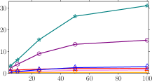
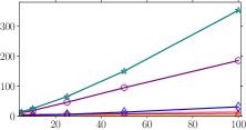
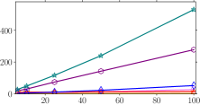
Cutoff $K$	Cutoff $K$	Cutoff $K$

Figure 1. Mean number of minutes required to complete one training epoch as $K$ varies on three datasets.

Yahoo! Webscope-Set1	MSLR-Web30k	Istella
$K=5$ NDCG@5
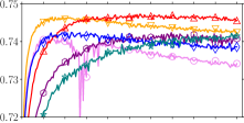
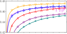
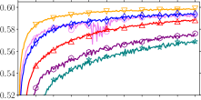
$K=10$ NDCG@10
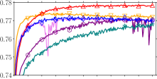
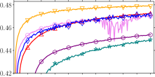
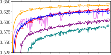
$K=25$ NDCG@25
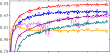
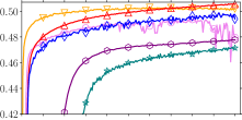
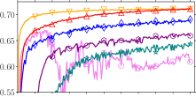
$K=50$ NDCG@50
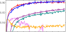
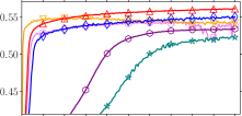
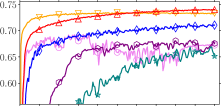
$K=100$ NDCG@100
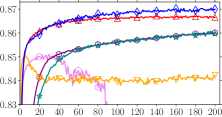
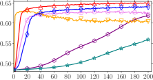
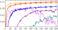
Minutes Trained	Minutes Trained	Minutes Trained

Figure 2. NDCG@K performance of PL-Rank-2, PL-Rank-3 and StochasticRank with $N=100$ and $N=1000$ when trained up to 200 minutes and for various $K$ values evaluated on the test-set of three datasets. All displayed results are averages over 30 independent runs. NDCG was normalized on dataset-level instead of query-level (Ferrante et al., 2021).

Table 2. Mean number of minutes taken to complete one epoch with various methods, ranking length/cutoff $K$ and number of samples $N$ on three datasets. Bold numbers indicate the minimal time per $N$ and $K$ values on each dataset.

	method	$N$	$K=5$	$K=10$	$K=25$	$K=50$	$K=100$
Yahoo!	Stoc.Rank	1100	0.52	0.80	1.64	2.58	3.01
		1000	3.38	6.18	15.41	26.17	31.03
	PL-Rank-2	1100	0.43	0.58	0.96	1.35	1.50
		1000	2.41	4.13	8.96	13.30	15.19
	PL-Rank-3	1100	0.33	0.34	0.38	0.40	0.40
		1000	1.33	1.53	1.92	2.18	2.19
MSLR	Stoc.Rank	1100	1.55	2.53	6.01	13.23	31.12
		1000	14.15	25.46	65.25	150.00	353.01
	PL-Rank-2	1100	1.19	1.75	4.04	8.36	15.71
		1000	10.34	18.91	46.27	94.81	185.42
	PL-Rank-3	1100	0.74	0.77	0.86	1.00	1.20
		1000	4.77	5.09	5.93	7.31	9.37
Istella	Stoc.Rank	1100	2.79	4.61	10.75	22.25	51.94
		1000	27.34	49.07	116.73	240.40	531.09
	PL-Rank-2	1100	1.96	2.87	6.72	13.25	27.07
		1000	18.49	30.37	74.09	142.55	278.01
	PL-Rank-3	1100	1.24	1.26	1.34	1.46	1.72
		1000	9.93	10.14	10.87	12.20	14.75

3. Method: A Faster PL-Rank Algorithm

We will now introduce PL-Rank-3: an algorithm for computing the same approximation as PL-Rank-2 but with a significantly better computational complexity. Algorithm 1 displays PL-Rank-3 in pseudo-code, we will now show that it produces the same approximation as PL-Rank-2 (cf. Algorithm 1 in (Oosterhuis, 2021)).

To start, we define $PR_{y,i}$ as the placement reward, the reward following the item placed at rank $i$ in ranking $y$:

(2) $$PR_{y,i}=\sum_{k=i}^{\min(i,K)}\theta_{k}\rho_{y_{k}},\quad PR_{y,d}=PR_{y,rank(d,y)+1}.$$

Importantly, all $PR_{y,i}$ values for a ranking can be computed in $K$ steps (Line 9). Next, we point out that a summation over item placement probabilities similar to Eq. 1 can be formulated as:

(3) $$\sum_{k=1}^{\text{rank}(d,y)}\pi(d\mid y_{1:k-1})=e^{f(d)}\left(\sum_{k=1}^{\text{rank}(d,y)}\frac{1}{\sum_{d^{\prime}\in D\setminus y_{1:k-1}}e^{f(d^{\prime})}}\right).$$

Using this insight, we define $RI_{y,i}$ to later compute the risk imposed by items with a non-zero placement probability at rank $i$ in $y$:

(4) $$RI_{y,i}=\sum_{k=1}^{\min(i,K)}\frac{PR_{y,k}}{\sum_{d^{\prime}\in D\setminus y_{1:k-1}}e^{f(d^{\prime})}},\quad RI_{y,d}=RI_{y,\text{rank}(d,y)}.$$

Similarly, we define $DR_{y,i}$ to compute the expected direct reward:

(5) $$DR_{y,i}=\sum_{k=1}^{\min(i,K)}\frac{\theta_{k}}{\sum_{d^{\prime}\in D\setminus y_{1:k-1}}e^{f(d^{\prime})}},\;DR_{y,d}=DR_{y,\text{rank}(d,y)}.$$

Crucial is that all $RI_{y,i}$ and $DR_{y,i}$ values can also be computed in $K$ steps (Line 12 & 13). With these newly defined variables, we can reformulate Eq. 1 without any summation over $K$:

(6) $$\frac{\delta\mathcal{R}(q)}{\delta f(d)}=\mathbb{E}_{y}\left[PR_{y,d}+e^{f(d)}\big{(}\rho_{d}DR_{y,d}-RI_{y,d}\big{)}\right].$$

Accordingly, Algorithm 1 approximates the gradient using:

(7) $$\begin{split}\frac{\delta\mathcal{R}(q)}{\delta f(d)}\approx&\frac{1}{N}\sum_{i=1}^{N}\left(PR_{y^{(i)},d}+e^{f(d)}\left(\rho_{d}DR_{y^{(i)},d}-RI_{y^{(i)},d}\right)\right).\end{split}$$

PL-Rank-3 computes the $PR$, $RI$ and $DR$ values in $K$ steps and then reuses them for each of the $D$ items, resulting in a computational complexity of $\mathcal{O}(N(D+K))$ given $N$ sampled rankings. However, when we consider that sampling a ranking relies on (partial) sorting, the full complexity of applying PL-Rank-3 becomes $\mathcal{O}(N(D+K\log(D))$.

Table 1 reveals that - to the best of our knowledge - PL-Rank-3 has the best computational complexity of all metric-based LTR methods. Moreover, because its computational complexity is limited by the underlying sorting procedure, we posit that PL-Rank-3 has reached the minimum order of computational complexity that is possible for a LTR method that is based on the full-ranking behavior of the model it optimizes.

4. Experimental Setup

We experimentally evaluate how the improvements in computational complexity translate to improvements in practical costs. Our experimental runs optimize the $DCG@K$ of neural ranking models on the Yahoo! Webscope-Set1 (Chapelle and Chang, 2011), MSLR-Web30k (Qin and Liu, 2013) and Istella (Dato et al., 2016) datasets. The neural models have two-hidden layers of 32 sigmoid activation nodes, backpropagation via standard gradient descent with a learning rate of $0.01$ was applied using Tensorflow (Abadi et al., 2016). We compare our PL-Rank-3 algorithm, with PL-Rank-2 (Oosterhuis, 2021) and StochasticRank (Ustimenko and Prokhorenkova, 2020). StochasticRank was chosen as a baseline because it shares many properties with PL-Rank (see Table 1) yet was not compared with PL-Rank in previous work (Oosterhuis, 2021). Our StochasticRank implementation uses the Gumbel distribution as stochastic noise instead of the normal distribution of the original algorithm (Ustimenko and Prokhorenkova, 2020), this makes the method applicable and effective to optimize a PL model. We reimplemented the PL-Rank and StochasticRank algorithms in Numpy (Harris et al., 2020) and performed all our experiments on AMD EPYC™ 7H12 CPUs. The ranking length/metric cutoff was varied: $K\in\{5,10,25,50,100\}$ and number of sampled rankings: $N\in\{100,1000\}$, to measure their impact on computational costs. Performance was measured over 200 minutes of training time, in addition to the average time required to complete one training epoch. All reported results are averages over 30 independent runs performed under identical circumstances. We report Normalized $DCG@K$ (NDCG@K) as our ranking performance metric computed on the held-out test-set of each dataset; following the advice of Ferrante et al. (2021), we do not use query-normalization but dataset-normalization: we divide the $DCG@K$ of a ranking model by the maximum possible $DCG@K$ value on the entire test-set of the dataset.

5. Results

Figure 1 and Table 2 shows the effect of ranking length $K$ on the computational costs of the LTR methods. As expected, Figure 1 reveals that PL-Rank-2 and StochasticRank are heavily affected by increases in $K$: there appears to be a clear linear trend on the MSLR and Istella datasets. We note that many queries in the Yahoo! dataset have less than 100 documents ($D\leq 100$) which could explain why the effect is sub-linear on that dataset. In contrast, PL-Rank-3 appears barely affected by $K$ on all of the datasets.

Table 2 allows us to also compare the computational costs in more detail. Regardless of whether $N=100$ or $N=1000$, the required times of PL-Rank-2 and StochasticRank scale close to linearly with $K$, but those for PL-Rank-3 do not. For instance, on Istella with $N=100$ and $K=5$, PL-Rank-2 needs 1.96 minutes, StochasticRank needs 2.79 and PL-Rank-3 needs 1.24 minutes, when compared to $K=100$, PL-Rank-2 needs an additional 25 minutes, StochasticRank 49 minutes more but PL-Rank-3 only requires an increase of 28 seconds. Moreover, PL-Rank-3 has the lowest computational costs when compared to the other methods with the same $N$ and $K$ values, across all three datasets. We thus conclude that in terms of time required to complete a single epoch, PL-Rank-3 is a clear improvement over PL-Rank-2 and StochasticRank. Additionally, in terms of scalability of computational costs w.r.t. $K$, PL-Rank-3 is the best choice by a considerable margin.

Now that we have established that PL-Rank-3 completes training epochs considerably faster than the other methods, we consider its effect on how quickly certain performance can be reached. Figure 2 show the performance of the LTR methods when optimizing $DCG@K$ over 200 minutes for various $K$ values. In all but two scenarios, PL-Rank-3 provides the highest performance at all times, where it seems to mostly depend on $K$ whether $N=100$ or $N=1000$ is a better choice. In particular, when $K\in\{5,10\}$ PL-Rank-3 with $N=100$ has the highest performance on MSLR and Istella and is only outperformed by PL-Rank-3 with $N=1000$ on Yahoo! Conversely, when $K\in\{50,100\}$, $N=1000$ is the better choice for PL-Rank-3 on all datasets. This suggests that gradient estimation for larger values of $K$ is more prone to variance and thus requires more samples for stable optimization. Overall, PL-Rank-2 appears very affected by variance across datasets and $K$ values, we mostly attribute this to the small number of epochs it can complete in 200 minutes. For example, on Istella with $K=100$, PL-Rank-2 completes less than eight epochs whereas PL-Rank-3 can complete 116 epochs. Interestingly, StochasticRank with $N=100$ has stable performance that is sometimes comparable with PL-Rank-3 with $N=1000$ on the Yahoo! dataset. This indicates that the sample-efficiency of StochasticRank is actually better than PL-Rank-3, however, due to its low computational costs, PL-Rank-3 still outperforms it on MSLR and Istella and when $K\in\{5,10,20\}$ on Yahoo! We conclude that PL-Rank-3 provides a clear and substantial improvement over PL-Rank-2, and in most scenarios also outperforms StochasticRank.

6. Conclusion

We have introduced PL-Rank-3 an LTR algorithm to estimate the gradient of a PL ranking model with the same computational complexity as the best sorting algorithms. PL-Rank-3 could enable future metric-based LTR to be applicable to ranking lengths and item collection sizes of much larger scales than previously feasible.

Code and data

To facilitate reproducibility, this work only made use of publicly available data and our experimental implementation is publicly available at https://github.com/HarrieO/2022-SIGIR-plackett-luce.

- (1)
- Abadi et al. (2016) Martín Abadi, Paul Barham, Jianmin Chen, Zhifeng Chen, Andy Davis, Jeffrey Dean, Matthieu Devin, Sanjay Ghemawat, Geoffrey Irving, Michael Isard, et al. 2016. Tensorflow: A System for Large-Scale Machine Learning. In 12th USENIX symposium on operating systems design and implementation OSDI’16). 265–283.
- Bruch et al. (2020) Sebastian Bruch, Shuguang Han, Michael Bendersky, and Marc Najork. 2020. A Stochastic Treatment of Learning to Rank Scoring Functions. In Proceedings of the 13th International Conference on Web Search and Data Mining. 61–69.
- Bruch et al. (2019) Sebastian Bruch, Masrour Zoghi, Michael Bendersky, and Marc Najork. 2019. Revisiting Approximate Metric Optimization in the Age of Deep Neural Networks. In Proceedings of the 42nd International ACM SIGIR Conference on Research and Development in Information Retrieval. 1241–1244.
- Burges (2010) Christopher J.C. Burges. 2010. From RankNet to LambdaRank to LambdaMART: An Overview. Technical Report MSR-TR-2010-82. Microsoft.
- Cao et al. (2007) Zhe Cao, Tao Qin, Tie-Yan Liu, Ming-Feng Tsai, and Hang Li. 2007. Learning to Rank: From Pairwise Approach to Listwise Approach. In Proceedings of the 24th international conference on Machine learning. 129–136.
- Chapelle and Chang (2011) Olivier Chapelle and Yi Chang. 2011. Yahoo! Learning to Rank Challenge Overview. Journal of Machine Learning Research 14 (2011), 1–24.
- Dato et al. (2016) Domenico Dato, Claudio Lucchese, Franco Maria Nardini, Salvatore Orlando, Raffaele Perego, Nicola Tonellotto, and Rossano Venturini. 2016. Fast Ranking with Additive Ensembles of Oblivious and Non-Oblivious Regression Trees. ACM Transactions on Information Systems (TOIS) 35, 2 (2016), Article 15.
- Diaz et al. (2020) Fernando Diaz, Bhaskar Mitra, Michael D. Ekstrand, Asia J. Biega, and Ben Carterette. 2020. Evaluating Stochastic Rankings with Expected Exposure. In Proceedings of the 29th ACM International Conference on Information & Knowledge Management. Association for Computing Machinery, New York, NY, USA, 275–284.
- Ferrante et al. (2021) Marco Ferrante, Nicola Ferro, and Norbert Fuhr. 2021. Towards Meaningful Statements in IR Evaluation: Mapping Evaluation Measures to Interval Scales. IEEE Access 9 (2021), 136182–136216.
- Fuhr (1989) Norbert Fuhr. 1989. Optimum Polynomial Retrieval Functions Based on the Probability Ranking Principle. ACM Transactions on Information Systems (TOIS) 7, 3 (1989), 183–204.
- Gumbel (1954) Emil Julius Gumbel. 1954. Statistical Theory of Extreme Values and Some Practical Applications: A Series of Lectures. Vol. 33. US Government Printing Office.
- Harris et al. (2020) Charles R. Harris, K. Jarrod Millman, St’efan J. van der Walt, Ralf Gommers, Pauli Virtanen, David Cournapeau, Eric Wieser, Julian Taylor, Sebastian Berg, Nathaniel J. Smith, Robert Kern, Matti Picus, Stephan Hoyer, Marten H. van Kerkwijk, Matthew Brett, Allan Haldane, Jaime Fern’andez del R’ıo, Mark Wiebe, Pearu Peterson, Pierre G’erard-Marchant, Kevin Sheppard, Tyler Reddy, Warren Weckesser, Hameer Abbasi, Christoph Gohlke, and Travis E. Oliphant. 2020. Array Programming with NumPy. Nature 585, 7825 (2020), 357–362.
- Järvelin and Kekäläinen (2002) Kalervo Järvelin and Jaana Kekäläinen. 2002. Cumulated Gain-Based Evaluation of IR Techniques. ACM Transactions on Information Systems (TOIS) 20, 4 (2002), 422–446.
- Joachims (2002) Thorsten Joachims. 2002. Optimizing Search Engines Using Clickthrough Data. In Proceedings of the eighth ACM SIGKDD international conference on Knowledge discovery and data mining. ACM, 133–142.
- Liu (2009) Tie-Yan Liu. 2009. Learning to Rank for Information Retrieval. Foundations and Trends in Information Retrieval 3, 3 (2009), 225–331.
- Luce (2012) R Duncan Luce. 2012. Individual Choice Behavior: A Theoretical Analysis. Courier Corporation.
- Moffat et al. (2017) Alistair Moffat, Peter Bailey, Falk Scholer, and Paul Thomas. 2017. Incorporating User Expectations and Behavior into the Measurement of Search Effectiveness. ACM Transactions on Information Systems (TOIS) 35, 3 (2017), 1–38.
- Oosterhuis (2021) Harrie Oosterhuis. 2021. Computationally Efficient Optimization of Plackett-Luce Ranking Models for Relevance and Fairness. In Proceedings of the 44th International ACM SIGIR Conference on Research and Development in Information Retrieval (Virtual Event, Canada) (SIGIR ’21). ACM, 1023–1032.
- Plackett (1975) Robin L Plackett. 1975. The Analysis of Permutations. Journal of the Royal Statistical Society: Series C (Applied Statistics) 24, 2 (1975), 193–202.
- Qin and Liu (2013) Tao Qin and Tie-Yan Liu. 2013. Introducing LETOR 4.0 datasets. arXiv preprint arXiv:1306.2597 (2013).
- Qin et al. (2021) Zhen Qin, Le Yan, Honglei Zhuang, Yi Tay, Rama Kumar Pasumarthi, Xuanhui Wang, Mike Bendersky, and Marc Najork. 2021. Are Neural Rankers still Outperformed by Gradient Boosted Decision Trees?. In 9th International Conference on Learning Representations, ICLR 2021, Virtual Event, Austria, May 3-7, 2021. OpenReview.net. https://openreview.net/forum?id=Ut1vF_q_vC
- Taylor et al. (2008) Michael Taylor, John Guiver, Stephen Robertson, and Tom Minka. 2008. Softrank: Optimizing Non-Smooth Rank Metrics. In Proceedings of the 2008 International Conference on Web Search and Data Mining. 77–86.
- Ustimenko and Prokhorenkova (2020) Aleksei Ustimenko and Liudmila Prokhorenkova. 2020. StochasticRank: Global Optimization of Scale-Free Discrete Functions. In International Conference on Machine Learning. PMLR, 9669–9679.
- Wang et al. (2018) Xuanhui Wang, Cheng Li, Nadav Golbandi, Michael Bendersky, and Marc Najork. 2018. The LambdaLoss Framework for Ranking Metric Optimization. In Proceedings of the 27th ACM International Conference on Information and Knowledge Management. ACM, 1313–1322.
- Xia et al. (2008) Fen Xia, Tie-Yan Liu, Jue Wang, Wensheng Zhang, and Hang Li. 2008. Listwise Approach to Learning to Rank: Theory and Algorithm. In Proceedings of the 25th international conference on Machine learning. 1192–1199.