Exploiting complex pattern features for interactive pattern mining

Abstract

Recent years have seen a shift from a pattern mining process that has users define constraints before-hand, and sift through the results afterwards, to an interactive one. This new framework depends on exploiting user feedback to learn a quality function for patterns. Existing approaches have a weakness in that they use static pre-defined low-level features, and attempt to learn independent weights representing their importance to the user. As an alternative, we propose to work with more complex features that are derived directly from the pattern ranking imposed by the user. Learned weights are then aggregated onto lower-level features and help to drive the quality function in the right direction. We explore the effect of different parameter choices experimentally and find that using higher-complexity features leads to the selection of patterns that are better aligned with a hidden quality function while not adding significantly to the run times of the method.

Getting good user feedback requires to quickly present diverse patterns, something that we achieve but pushing an existing diversity constraint into the sampling component of the interactive mining system LetSIP. Resulting patterns allow in most cases to converge to a good solution more quickly.

Combining the two improvements, finally, leads to an algorithm showing clear advantages over the existing state-of-the-art.

1 Introduction

Constraint-based pattern mining is a fundamental data mining task, extracting locally interesting patterns to be either interpreted directly by domain experts, or to be used as descriptors in downstream tasks, such as classification or clustering. Since the publication of the seminal paper Agrawal94 , two problems have limited the usability of this approach: 1) how to translate user preferences and background knowledge into constraints, and 2) how to deal with the large result sets that often number in the thousands or even millions of patterns. Replacing the original support-confidence framework with other quality measures DBLP:conf/kdd/TanKS02 does not address the pattern explosion. Post-processing results via condensed representations Lakhal still typically leaves many patterns, while pattern set mining DBLP:conf/sdm/RaedtZ07 just pushes the problem further down the line.

In recent years, research on interactive pattern mining has proposed to alter the mining process itself: instead of specifying constraints once, mining a result set, and then post-processing it, interactive pattern mining performs an iterative loop DBLP:conf/icml/Rueping09 . This loop involves three repeating main steps: (1) pattern extraction in which a relatively small set of patterns is extracted; (2) interaction in which the user expresses his preferences w.r.t. those patterns; (3) preference learning in which the expressed preferences are translated into a quality assessment function for mining patterns in future iterations.

Existing approaches DBLP:conf/icml/Rueping09 ; Dzyuba:letsip ; DBLP:journals/sadm/BhuiyanH16 have a short-coming, however: to enable preference learning, they represent patterns by independent descriptors, such as included items or covered transactions, and expect the learned function, usually a regression or multiplicative weight model, to handle relations. Furthermore, to get quality feedback, it is important to present diverse patterns to the user, an aspect that is at best indirectly handled by existing work.

The contributions of this paper are the following:

1. We introduce cdFlexics, which improves the pattern sampling method proposed in Dzyuba:flexics , Flexics, by integrating closedDiversity into it to extract patterns. This will allow us to exploit both the sampling and the $XOR$ constraints of Flexics which has the advantage that it is anytime, as well as the filtering of ClosedDiv to maximize patterns diversity.

2. We extend a recent interactive pattern mining approach (LetSIP Dzyuba:letsip ) by introducing new, more complex, descriptors for explainable ranking, thereby leading to a more concise and diverse pattern sets. These descriptors exploit the concept of discriminating sub-patterns, which separate patterns that are given low rank by the user from those with high rank. By temporarily adding those descriptors, we can learn weights for them, which are then apportioned to involved items without blowing up the feature space.

3. We combine those two improvements to LetSIP, i.e. the improved sampling of cdFlexics and the more complex features learned dynamically during the iterative mining process. This allows the resulting algorithm to both return more diverse patterns more efficiently, and to leverage user feedback more effectively to improve later iterations.

In Section 3, we discuss how we integrate closedDiversityinto Flexics. In Section 4, we explain how to derive complex pattern features, followed by a discussion of how to map user feedback back into primitive features. Section 6 containts extensive experiments evaluating our contributions, before we discuss related work in Section 7. We conclude in Section 8.

2 Preliminaries

Algorithm 1 The general CP solving algorithm

1:function Solve($\mathcal{S}=\left<X,D,\mathcal{C}\right>$)

2:     Begin

3:         $\textsc{Propagate}(\mathcal{S})$

4:         if $\exists x_{i}\in X\,s.t.\,\lvert dom(x_{i})\rvert=0$ then

5:              return $\emptyset$

6:         else if $\exists x_{i}\in X\,s.t.\,\lvert dom(x_{i})\rvert>1$ then

7:              $d\leftarrow\textsc{MakeDecision}(\mathcal{P})$  

8:              return $\textsc{Solve}(\mathcal{P}\land d)\cup\textsc{Solve}(\mathcal{P}\land\lnot d)$

9:         else

10:              return solution $D$

11:         end if

12:     End

13:end function

2.1 Constraint Programming (CP)

Constraint programming HoeveK06 is a powerful paradigm which offers a generic and modular approach to model and solve combinatorial problems. A CP model consists of a set of variables $X=\{x_{1},\ldots,x_{n}\}$, a set of domains $D$ mapping each variable $x_{i}\in X$ to a finite set of possible values $dom(x_{i})$, and a set of constraints $\mathcal{C}$ on $X$. A constraint $c\in\mathcal{C}$ is a relation that specifies the allowed combinations of values for its variables $X(c)$. An assignment on a set $Y\subseteq X$ of variables is a mapping from variables in $Y$ to values in their domains. A solution is an assignment on $X$ satisfying all constraints.

To find solutions, CP solvers usually work in two steps. First, the search space is reduced by adding constraints (called decisions) in a depth-first search. A decision is, for example, an assignment of a variable to a value in its domain. Then comes a phase of propagation that checks the satisfiability of the constraints of the CP model. This phase can also filter (i.e. remove) values in the domains of variables that do not lead to solutions . At each decision, constraint filtering algorithms prune the search space by enforcing local consistency properties like domain consistency. A constraint $c$ on $X(c)$ is domain consistent, if and only if, for every $x_{i}\in X(c)$ and every $v\in dom(x_{i})$, there is an assignment satisfying $c$ such that $(x_{i}=v)$. The baseline recursive algorithm for solving is presented in Algorithm 1. It relies on the two functions Propagate and MakeDecision to respectively filter values by using constraints and reduce the search space by making decisions.

2.2 Pattern mining

Given a database $\mathcal{D}$, a language ${\cal L}$ defining subsets of the data and a selection predicate $q$ that determines whether an element $\phi\in{\cal L}$ (a pattern) describes an interesting subset of $\mathcal{D}$ or not, the task is to find all interesting patterns, that is,

$$\mathcal{T}({\cal L},\mathcal{D},q)=\{\phi\in{\cal L}\mid\,\,q(\mathcal{D},\phi)\,\,is\,\,true\}$$

A well-known pattern mining task is frequent itemset mining Agrawal94 . Let $\mathcal{I}=\{1,...,n\}$ be a set of $n$ items, an itemset (or pattern) $P$ is a non-empty subset of $\mathcal{I}$. The language of itemsets corresponds to ${\cal L}_{\mathcal{I}}=2^{\mathcal{I}}\backslash\emptyset$. A transactional dataset $\mathcal{D}$ is a bag (or multiset) of transactions over $\mathcal{I}$, where each transaction $t$ is a subset of $\mathcal{I}$, i.e., $t\subseteq\mathcal{I}$; $\mathcal{T}=\{1,...,m\}$ a set of $m$ transaction indices. An itemset $p$ occurs in a transaction $t$, iff $p\subseteq t$. The cover of $p$ in $\mathcal{D}$ is the bag of transactions in which it occurs: $\mathcal{V}_{\mathcal{D}}(p)=\{t\in\mathcal{D}{}\mid p\subseteq t\}$. The support of $p$ in $\mathcal{D}$ is the size of its cover: $sup_{\mathcal{D}}(p)$ = $\lvert\mathcal{V}_{\mathcal{D}}(p)\rvert$. A well-known interestingness predicate is a threshold on the support of the itemsets, the minimal support: $\theta$. The task in frequent set mining is to compute frequent itemsets: $\{p\in{\cal L}_{\mathcal{I}}\mid\,\,sup_{\mathcal{D}}(p)\geq\theta\}$.,

Additional constraints on the individual itemsets to reduce the redundancy between patterns, such as closed frequent itemsetsLakhal , have been proposed. An itemset $p$ is said to be closed if there is no $q\supseteq p$ such that $sup_{\mathcal{D}}(p)=sup_{\mathcal{D}}(q)$, that is, $p$ is maximal with respect to set inclusion among those itemsets having the same support.

Constraint Programming for Itemset Mining. Several proposals have investigated relationships between itemset mining and constraint programming (CP) to revisit data mining tasks in a declarative and generic way BelaidBL19a ; LazaarLLMLBB16 ; RaedtGN08 ; SchausAG17 ; KhiariBC10 . The declarative aspect represents the key advantage of the proposed CP approaches. This allows modeling of complex user queries without revising the solving process but at the cost of efficiency.

A CP model for mining frequent closed itemsets was proposed in LazaarLLMLBB16 which has successfully encoded both the closeness relation as well as the anti-monotonicity of frequency into one global constraint called closedPattern. It uses a vector of Boolean variables $(x_{1},\ldots,x_{\lvert\mathcal{I}\rvert})$ for representing itemsets, where $x_{i}$ represents the presence of the item $i\in\mathcal{I}$ in the itemset. We will use the notation $x^{+}=\{i\in\mathcal{I}\,\mid\,x_{i}=1\}$ to represent the pattern associated to these variables.

Definition 1 (closedPattern constraint).

Let $(x_{1},\ldots,x_{\lvert\mathcal{I}\rvert})$ be a vector of Boolean variables, $\theta$ a support threshold and $\mathcal{T}$ a dataset. The constraint $\textsc{closedPattern}_{\mathcal{D},\theta}(x_{1},\ldots,x_{\lvert\mathcal{I}\rvert})$ holds if and only if $x^{+}$ is a closed frequent itemset w.r.t. the threshold $\theta$.

2.3 Pattern Diversity

The discovery of a set of diverse itemsets from binary data is an important data mining task. Different measures have been proposed to measure the diversity of itemsets. In this paper, we consider the Jaccard index as a measure of similarity on sets. We use it to quantify the overlap of the covers of itemsets.

Definition 2 (Jaccard index).

Let $p$ and $q$ be two itemsets. The Jaccard index is defined as

$$Jac(p,q)=\frac{\lvert\mathcal{V}_{\mathcal{D}}{p}\cap\mathcal{V}_{\mathcal{D}}{q}\rvert}{\lvert\mathcal{V}_{\mathcal{D}}{p}\cup\mathcal{V}_{\mathcal{D}}{q}\rvert}$$

A lower Jaccard indicates low similarity between itemset covers, and can thus be used as a measure of diversity between pairs of itemsets.

Definition 3 (Diversity/Jaccard constraint).

Let $p$ and $q$ be two itemsets. Given the $Jac$ measure and a diversity threshold $J_{max}$, we say that $p$ and $q$ are pairwise diverse iff $Jac(p,q)\leq J_{max}$.

We now formalize the diversity problem for itemset mining. Diversity is controlled through a threshold on the Jaccard similarity of pattern occurrences.

Definition 4 (Diverse frequent itemsets).

Let $\mathcal{H}$ be a history of pairwise diverse frequent itemsets, and $J_{max}$ a bound on the maximum allowed Jaccard value. The task is to mine new itemsets $p$ such that $p$ is diverse according to $\mathcal{H}$:

$$\texttt{div}_{J}(p,\mathcal{H},J_{max})\Leftrightarrow\forall h\in\mathcal{H},Jac(p,h)\leq J_{max}$$

In HienLALLOZ20 , we showed that the Jaccard index has no monotonicity property, which prevents usual pruning techniques and makes classical pattern mining unworkable. To cope with the non-monotonicity of the Jaccard similarity, we proposed an anti-monotonic lower bound relaxation of the Jaccard index, which allow effective pruning.

Proposition 1 (Lower bound).

Let $p$ and $h$ be two patterns, and $\theta$ a bound on the minimal frequency of the patterns, then

$$LB(p,h)=\frac{\max(0,\theta-\lvert\mathcal{V}_{\mathcal{D}}(p)\backslash\mathcal{V}_{\mathcal{D}}(h)\rvert}{\lvert\mathcal{V}_{\mathcal{D}}(h)\rvert+\lvert\mathcal{V}_{\mathcal{D}}(p)\backslash\mathcal{V}_{\mathcal{D}}(h)\rvert}\leq Jac(p,h)$$

This Approximate bound is then exploited within the closedPattern constraint to mine pairwise diverse frequent closed itemsets.

Definition 5 (closedDiversity).

Let $x$ be a vector of Boolean item variables, $\mathcal{H}$ a history of pairwise diverse frequent closed itemsets (initially empty), $\theta$ a support threshold, $J_{max}$ a bound on the maximum allowed Jaccard, and $\mathcal{D}$ a dataset. The $\textsc{closedDiversity}_{\mathcal{D},\theta}(x,\mathcal{H},J_{max})$ constraint holds if and only if: (1) $x^{+}$ is closed; (2) $x^{+}$ is frequent, $sup_{\mathcal{D}}(x^{+})\geq\theta$; (3) $x^{+}$ is diverse, $\forall\,h\in\mathcal{H},LB(x^{+},h)\leq J_{max}$.

By using this lower bound, it is easier to filter items that would give patterns too close to the ones in the history (see HienLALLOZ20 for more details).

2.4 LetSIP: Weighted constrained sampling

Our work is based on LetSIP Dzyuba:letsip , which in turn uses Flexics Dzyuba:flexics . In this and the next section, we will therefore sketch the pattern sampling and feedback + preference learning steps of LetSIP (see Algorithm 3) before describing our own proposals in Sections 3 and 4. The main idea behind Flexics consists of partitioning the search space into a number of cells, and then sampling a solution from a random cell. This technique was inspired by recent advances in weighted solution sampling for SAT problems SatSampling-AAAI15 . It exploits Weightgen DBLP:journals/corr/ChakrabortyFMSV14 to sample SAT problem solutions. Weightgen partitions the search space into cells using random XOR constraints and then extracts a pattern from a randomly selected cell. An individual XOR constraint over variables X has the form $\bigotimes b_{i}.x_{i}=b_{0}$, where $b_{0\mid i}\in\{0,1\}$. The coefficients $b_{i}$ determine the variables involved in the constraint, whereas the parity bit $b_{0}$ determines whether an even or an odd number of variables must be set to $1$. Together, $m$ XOR constraints identify one cell belonging to a partitioning of the overall solution space into $2^{m}$ cells. Weightgen uses a two-step procedure consisting of 1) estimating the number of XOR required for the partitioning and 2) generating these random constraints and sample the solutions. The sampling step needs the use of an efficient oracle to enumerate the solutions in the different cells. Dzyuba et al. evaluated two oracles: EFlexics which employs the Eclat Algorithm for the enumeration and GFlexics, a CP-based method based on CP4IM RaedtGN08 . In this paper, we propose to use an efficient CP-based method, called cdFlexics, based the closedDiversityglobal constraint.

2.5 LetSIP: Preference based pattern mining

User feedback w.r.t. patterns takes the form of providing a total order over a (small) set of patterns, called a query $Q$. User feedback $\{p_{1}\succ p_{3}\succ p_{2}\succ p_{4}\}$, for instance, indicates that the user prefers $p_{1}$ over $p_{3}$, which they prefer over $p_{2}$ in turn, and so on. This total order is translated into pairwise rankings $\{(p_{1}\succ p_{3}),(p_{1}\succ p_{2}),(p_{1}\succ p_{4}),\ldots\}$. Patterns are represented using a feature representation $\mathbf{F}=\{f_{1},\ldots,f_{d}\}\in\mathbb{R}^{d}$. Examples of features include $Len(p)=\lvert p\rvert/\lvert\mathcal{I}\rvert$, $Freq(p)=sup_{\mathcal{D}}(p)/\lvert\mathcal{D}\rvert$, in which case the corresponding $f_{i}$ is truly in $\mathbb{R}$, or $Items(i,p)=[i\in p]$; and $Trans(t_{i},p)=[p\subseteq t_{i}]$, where $[.]$ denotes the Iverson bracket, leading to (partial) feature vectors $\in\{0,1\}^{\lvert\mathcal{I}\rvert}$ and $\in\{0,1\}^{\lvert\mathcal{D}\rvert}$, respectively. The total number of features depends on the dimensions of the data, and is equal to $\lvert\mathcal{I}\rvert+\lvert\mathcal{D}\rvert+2$. Given this feature representation, each ranked pair $p_{i}\succ p_{j}$ corresponds to a classification example $(\mathbf{F}_{i}-\mathbf{F}_{j},+)$.

LetSIP uses the parameterized logistic function

$$\phi_{logistic}(p\mathchar 24635\relax\;w,A)=A+\frac{1-A}{1+e^{-\mathbf{w\cdot{F}}}}$$

as a learnable quality function for patterns with $\mathbf{F}$ the aforementioned feature representation of a pattern $p$, $\mathbf{w}$ the weight vector to be learned, and $A$ is a parameter that controls the range of the interestingness measures, i.e. $\phi_{logistic}\in[A,1]$. For details, we direct the reader to the original publication Dzyuba:letsip . Finally, to select the $k$ patterns $Q$ to be presented to the user, LetSIP uses Flexics to sample $k$ patterns proportional to $\phi_{logistic}$. These patterns are selected according to a Top($m$) strategy, which picks the $m$ highest-quality patterns from a cell (Algorithm 3, line 31). Moreover, to help users to relate the queries to each other, LetSIP propose to retain the top $\ell$ patterns from the previous query and only sample $k-\ell$ new patterns  (Algorithm 3, lines 10-12).

Example 1.

Let $\mathcal{I}=\{0,\ldots,6\}$ be a set of items and $Q=\{p_{1},p_{2},p_{3},p_{4}\}$ a sample of $four$ patterns, where $p_{1}=\{4,6\},p_{2}=\{1,6\},p_{3}=\{0\}$ and $p_{4}=\{3\}$. Let’s consider a user ranking $U=\{p_{2}\succ p_{1}\succ p_{3}\succ p_{4}\}$ as feedback and suppose that $sup_{\mathcal{D}}(p_{1})=0.54$, $sup_{\mathcal{D}}(p_{2})=0.18$ and $sup_{\mathcal{D}}(p_{3})=0.36$. Using items and frequency as features, we have $\mathbf{F}_{1}=(0,0,0,0,1,0,1,0.54)$, $\mathbf{F}_{2}=(0,1,0,0,0,0,1,0.18)$, $\ldots$ To learn the vector of weights $\mathbf{w}$, $U$ is translated into pairwise rankings $\{$($p_{2}\succ p_{1}$), ($p_{2}\succ p_{3}$), $\ldots\}$ and distances between feature vectors for each pair are calculated. So, given the preference $p_{2}\succ p_{1}$, we have $\mathbf{F}_{2}-\mathbf{F}_{1}=(0,1,0,0,-1,0,0,-0.36)$. After the first iteration of LetSIP, the learned weight vector is $\mathbf{w}=(-0.33,0.99,0,-0.99,0.33,0,1.33,0.15)$.

3 Sampling Diverse Frequent Patterns

LetSIP’s sampling component is based on Flexics. An interactive system seeks to ensure faster learning of accurate models by targeted selection of patterns to show to the user. An important aspect is that the user be quickly presented with diverse results. If patterns are too similar to each other, deciding which one to prefer can become challenging, and if they appear in several successive iterations, it eventually becomes a slog.

We propose in this section a modification to Flexics, called cdFlexics, to explicitly control the diversity of sampled patterns, thus ensuring pattern diversity within each query and thus sufficient exploration. Our key idea is to exploit the diversity constraint closedDiversity as an oracle to select the patterns in the different cells (partitions). We start by presenting our strategy for integrating closedDiversity into Flexicsin section 3.1, then we detail the associated filtering algorithm in section 3.2.

3.1 Integrating the diversity constraint into Flexics

In order to turn closedDiversity into a suitable oracle, we propose to control the diversity of patterns sampled from each cell as follows. We maintain a local history $\mathcal{H}_{loc}$ for each cell. Initially, $\mathcal{H}_{loc}$ is initialized to empty. Each time a new diverse pattern is mined from the current cell, it is added to $\mathcal{H}_{loc}$ and the exploration of the remaining search space of the cell continues using the new updated history. Finally, the pattern sampled for that cell is picked among the diverse patterns in $\mathcal{H}_{loc}$, with a probability proportional to a given quality measure, e.g., frequency. This process is repeated for each new cell until the required number of samples is reached. With a such strategy, the exploration of the different cells become more efficient and faster, as their size is greatly reduced thank to the filtering of closedDiversity which avoids the discovery of non diverse patterns within each cell.

$\left\{\begin{array}[]{l}x_{1}\oplus x_{5}=0\\ x_{1}\oplus x_{3}\oplus x_{5}=0\\ x_{4}\oplus x_{5}=1\\ \end{array}\right.$ 1) Random XOR Constraints

1 0 0 0 1 0 1 0 1 0 1 0 0 0 0 1 1 1 2) Initial constraint matrix

1 0 0 0 1 0 $\rightarrow$ 0 0 1 0 0 0  0 0 0 1 1 1 3) Echelonized matrix: $x_{3}=0$ is derived

1 0 0 0 1 0 0 0 0 1 1 1 0 0 0 0 0 0 4) Updated matrix (rows 2 and 3 are swapped)

$\downarrow$ $\downarrow$  1 0 0 0 0 1 $\rightarrow$ 0 0 0 0 0 1  0 0 0 0 0 0 5) If $x_{4}$ et $x_{5}$ are set to 1, the system is unsat.

Figure 1: Propagation example of XOR constraints using Gaussian elimination.

3.2 Filtering of cdFlexics

The filtering of cdFlexics combines two propagators, that of closedDiversity (see HienLALLOZ20 for more details) and the propagator for XOR constraints. In CP, constraints interact through shared variables, i.e., as soon as a constraint has been propagated (no more values can be pruned), and at least a value has been eliminated from the domain of a variable, say $v$, then the propagation algorithms of all other constraints involving $v$ are triggered. For instance, when the propagator of closedDiversity modifies the domain of item variables, these modifications must be propagated to XOR constraints. Now, we detail the filtering algorithm of the XOR constraints. This propagator is based on the method of Gaussian elimination GomesHSS07 , a classical algorithm for solving systems of linear equations. All coefficients $b_{i}\in\{0,1\}$ of the XOR constraints form a binary matrix $\mathcal{M}$ of size $(n,m+1)$, where $n$ is the number of Individual XOR constraints and $m$ is the number of items in the dataset, the last column $b_{0}\in\{0,1\}$ represents the parity bit. Thus, for each constraint XOR $k$, if a variable $x_{i}$ is involved in this constraint, then $\mathcal{M}[k,i]=1$, otherwise $\mathcal{M}[k,i]=0$. Figure 1.2 shows the augmented matrix representation of the XOR constraints system of Figure 1.1 on a dataset of $5$ items.

Algorithm 2 Filtering for XOR constraints

1:$\mbox{Coefficient matrix}\mathcal{M}$

2:Vector of Boolean variables $(x_{1}\ldots x_{n})$

3:Begin

4:    $x^{+}\leftarrow\{i|x_{i}=1\},\,x^{-}\leftarrow\{i|x_{i}=0\},\,x^{*}\leftarrow\{i|i\notin x^{+}\cup x^{-}\}$

5:    foreach ($i\in x^{+}\ \wedge\mbox{row}\ r\in\mathcal{M}$) do

6:        if ($\mathcal{M}[r][i]=1$) then

7:           $b_{0}^{r}\leftarrow$ $1-b_{0}^{r}$

8:        end if

9:        $\mathcal{M}[r][i]\leftarrow 0$

10:    end for

11:    if  CheckInconsistency() then return $fail$

12:    else if ($x^{*}=\emptyset$) then return $true$

13:    else

14:        Echlonize($\mathcal{M}$)

15:        if CheckInconsistency() then return $fail$

16:        else FixVariables()

17:        end if

18:    end if

19:    return $true$

20:End

21:function CheckInconsistency( )

22:    foreach $row$ $r\in\mathcal{M}$ do

23:        if ($b_{0}^{r}=1$ $\wedge$ $\sum_{i=1}^{n}{\mathcal{M}[r][i]}=0$) then

24:           return $true$

25:        end if

26:    end for

27:    return $false$

28:end function

29:procedure FixVariables( )

30:    foreach $row$ $r\in\mathcal{M}$ do

31:        if ($\sum_{i=1}^{n}{\mathcal{M}[r][i]}=1$) then

32:           $dom(x_{i})\leftarrow dom(x_{i})-\{1-b_{0}^{r}\}\mathchar 24635\relax\;$

33:           $x^{+}\leftarrow x^{+}\cup\{i\}$; $\vee$ $x^{-}\leftarrow x^{-}\cup\{i\}$

34:        end if

35:    end for

36:end procedure

At each step (see Algorithm 2), the matrix $\mathcal{M}$ is updated with the latest variable assignments $x^{+}$: for each variable $x_{i}$ set to $1$, the parity bit of the constraint where the variable appears is inverted and the coefficient of this variable in the matrix $\mathcal{M}$ is set to $0$. Figure 1.5 shows this transformation where the parity bit of line $1$ becomes 1 and the coefficient of variable $x_{5}$ is set $0$. Then, we check if the updated matrix does not lead to an inconsistency, i.e., if a row becomes empty while its right hand side is equal to $1$. In this case, the XOR constraints system is unsatisfiable and the current search branch terminates (Figure 1.5). Otherwise, an echelonization operation (line 14) is performed with the Gauss method to obtain an echelonized matrix : all ones are on or above the main diagonal and all non-zero rows are above any rows of all zero (Figure 1.3). During echelonization, two situations allow propagation. If a row becomes empty while its right hand side is equal to $1$, the system is unsatisfiable. If a row contains only one free variable, it is assigned the right hand side of the row (Figure 1.3).

Algorithm 3 LetSIP extension (new steps are in bold font)

1:Dataset $\mathcal{D}$, minimal frequency threshold $\theta$

2:Query of size $k$, number of iterations $T$, query retention $\ell$, range $A$, Flexics error tolerance $\kappa$, Patterns feature representations $\mathbf{F}$

3:Begin

4:    Weight vector $\mathbf{w}^{0}\leftarrow\mathbf{0}$,

5:    Feedback $U\leftarrow\emptyset$,

6:    Ranked patterns $Q_{0}^{*}\leftarrow\emptyset$

7:     $\ignorespaces\triangleright$ Initialization

8:    Ranking function $h_{0}\leftarrow\textsc{Logistic}(\mathbf{w}^{0},A)$

9:    for $t=1,2\ldots T$ do $\ignorespaces\triangleright$ Mine, Interact, Learn, Repeat loop

10:        $R\leftarrow\textsc{TakeFirst}(Q^{*}_{t-1},\ell)$

11:         $\ignorespaces\triangleright$ Retain the top $\ell$ patterns from the previous iteration

12:        Query $Q_{t}\leftarrow R\cup\textsc{SamplePatterns}(\mathcal{D},h_{t-1})\times(k-\lvert R\rvert)$

13:         $\ignorespaces\triangleright$ Call SamplePatterns $(k-\lvert R\rvert)$ times

14:        $\mathcal{P}_{t}\leftarrow\textsc{Rank}(Q_{t})$; $U\leftarrow U\cup\mathcal{P}_{t}$

15:         $\ignorespaces\triangleright$ Ask user to rank patterns in $Q_{t}$

16:        $\mathbf{F}\leftarrow\textsc{ConvertToFeaturesVectors}(\mathcal{P}_{t},\mathcal{D})$

17:         $\ignorespaces\triangleright$ Convert patterns to feature representations

18:        ${p_{disc}}\leftarrow$ LearnDiscriminatingPattern$(\mathcal{P}_{t})$

19:         $\ignorespaces\triangleright$ Extract discriminating pattern (Algorithm 4)

20:        $\mathbf{F}^{*}\leftarrow$ AddDiscrPatternFeature$(\mathbf{F},{p_{disc}},\mathcal{D})$

21:         $\ignorespaces\triangleright$ Update pattern features

22:        $\mathbf{w}^{t}\leftarrow$ Aggregate(LearnWeights$(U,\lambda,\mathbf{w}^{t-1},\mathbf{F}^{*}))$

23:         $\ignorespaces\triangleright$ Update pattern features weights

24:        $\mathbf{F}\leftarrow$ RemoveDiscrPatternFeature$(\mathbf{F}^{*},{p_{disc}},\mathcal{D})$

25:         $\ignorespaces\triangleright$ remove discr. pattern feature

26:        $h_{t}\leftarrow\textsc{Logistic}(\mathbf{w}^{t},A)$

27:    end for

28:End

29:function SamplePatterns($\mathcal{D}$, Sampling weight $\mathbf{w}:L\rightarrow[A,1]$)

30:    $C\leftarrow\textbf{{cdFlexics}}(\mathcal{D},freq(.)\geq\theta,\mathbf{w}\mathchar 24635\relax\;\kappa)$

31:    return Top($m$) highest-wheighted patterns from $C$

32:end function

4 Preference learning based on explainable ranking

4.1 Towards more expressive and learnable pattern representations

Features for pattern representation involve indicator variables for included items or sub-graphs, or for covered transactions Dzyuba:letsip ; DBLP:journals/sadm/BhuiyanH16 , or pattern length or frequency Dzyuba:letsip . The issue is that such features are treated as if they were independent, whether in the logistic function mentioned above, or multiplicative functions DBLP:conf/icml/Rueping09 ; DBLP:journals/sadm/BhuiyanH16 . While this allows to identify pattern components that are globally interesting for the user, it is impossible to learn relationships such as ”the user is interested in item $i_{1}$ if item $i_{3}$ is present but item $i_{4}$ is absent”. In addition, the pattern elements whose inclusion is indicated are defined before-hand, and the user feedback has no influence on them. We therefore propose to learn more expressive features in order to improve the learning of user preferences.

In this work, we propose to consider discriminating sub-patterns that better capture (or explain) these preferences. Those features exploit ranking-correlated patterns, i.e., patterns that influence the user ranking either by allowing some patterns to be well ranked or the opposite.

4.2 Interclass Variance

As explained above, our goal is to mine sub-patterns that discriminate between patterns that have been given a high user ranking and those that received a low one. An intuitive way of modelling this problem consists of considering the numerical ranks given to individual patterns as numerical labels and the mining setting as akin to regression. We are not aiming to build a full regression model but only to mine an individual pattern that correlates with the numerical label. For this purpose, we use the interclass variance measure as proposed by morishita .

Definition 6.

Let $\mathcal{P}$ be a set of ranked patterns of size $k$ according to user ranking $U$, and $\mathcal{P}^{*}$ be a subset of $\mathcal{P}$. We define by $\mu(\mathcal{P}^{*})$ the average rank of patterns $p\in\mathcal{P}^{*}$:

$$\mu(\mathcal{P}^{*})=\frac{1}{\lvert\mathcal{P}^{*}\rvert}\cdot\sum_{p\in\mathcal{P}^{*}}r(p),$$ (1)

where $r(p)$ is the rank of $p$ according to a user feedback.

Let $\mathcal{P}_{y}=\{p\in\mathcal{P}\,\lvert\,p\supseteq y\}$: the subset of patterns $p$ in $\mathcal{P}$ in which the sub-pattern $y$ is present, and $\overline{\mathcal{P}}_{y}=\mathcal{P}\backslash\mathcal{P}_{y}$. The interclass variance of the sub-pattern $y$ is defined by:

$$ICV(y)=\lvert\mathcal{P}_{y}\rvert\cdot(\mu(\mathcal{P})-\mu(\mathcal{P}_{y}))^{2}+\lvert\overline{\mathcal{P}}_{y}\rvert\cdot(\mu(\mathcal{P})-\mu(\overline{\mathcal{P}}_{y}))^{2}$$ (2)

The sub-pattern $y$ having the largest $ICV$ is then the one which is the most strongly correlated with the user ranking of the patterns.

Example 2.

Consider again our example with a query $Q=\{p_{1},p_{2},p_{3},p_{4}\}$ and the user feedback $U=\{p_{2}\succ p_{1}\succ p_{3}\succ p_{4}\}$. Let $\mathcal{P}$ the corresponding ranked patterns w.r.t. $U$. For $y=\{1\}$, we get $\mathcal{P}_{y}=\{p_{2}\}$ (since $\{1,6\}\supseteq\{1\}$), $\overline{\mathcal{P}}_{y}=\{p_{1},p_{3},p_{4}\}$, $\mu(\mathcal{P}_{y})=1$; $\mu(\overline{\mathcal{P}}_{y})=\frac{r(p_{1})+r(p_{3})+r(p_{4})}{3}=\frac{(2+3+4)}{3}=3$ and $\mu(\mathcal{P})=2.5$. Applying equation (2), we get $ICV(\{1\})=(2.5-1)^{2}+3\cdot(2.5-3)^{2}=3$. Similarly, $ICV(\{0\})=0.33$.

4.3 Learning Discriminating Sub-Patterns

To find the sub-pattern $y\subseteq p$ with the greatest interclass variance $ICV$ to be used as a new feature ($p\in\mathcal{P}$, st. $\mathcal{P}$ being the set of ranked patterns), we systematically search the pattern space spanned by the items involved in patterns in $\mathcal{P}$. Semantically, this is the sub-pattern whose presence in one or more itemsets $p$ has influenced their ranking. So, if $y\subseteq p$, we can say that the ranking of $p$ at the $i^{th}$ position in $\mathcal{P}$ is more likely to be explained by the presence of sub-pattern $y$.

Algorithm 4 The LearnDiscriminatingPattern algorithm

1:function LearnDiscriminatingPattern(set of ranked patterns $\mathcal{P}$)

2:    $ICV_{max}\leftarrow 0$, $p_{disc}\leftarrow\emptyset$

3:    $allItems\leftarrow items(\cup p\in\mathcal{P})$

4:    $subPatterns\leftarrow allItems$

5:    foreach $item\in allItems$ do

6:        if $ICV(item)\geq ICV_{max}$ then

7:           $ICV_{max}\leftarrow ICV(item)$

8:           $p_{disc}\leftarrow\{item\}$

9:        end if

10:    end for

11:    foreach $elt\in subPatterns$ do

12:        while ($(item\in allItems\backslash elt)\wedge(\exists p\in\mathcal{P}\;st.\;\{elt\cup item\}\subseteq p)$) do

13:           if $ICV(elt\cup item)\geq ICV_{max}$ then

14:               $ICV_{max}\leftarrow ICV(elt\cup\{item\})$

15:               $p_{disc}\leftarrow elt\cup\{item\}$

16:               $subPatterns\leftarrow subPatternss\cup\,p_{disc}$

17:           end if

18:        end while

19:    end for

20:    return $p_{disc}$

21:end function

Algorithm 4 implements the function LearnDiscriminatingPattern (see Algorithm 3, line 18), which learns the best discriminating pattern as a feature. Its accepts as input a set of ranked patterns $\mathcal{P}$, and returns the sub-itemset with the highest ICV. Its starts by calculating the $ICV$ of all items of the patterns $p\in\mathcal{P}$ (loop 5$-$10). Then, it iteratively combines the items to form a larger and finer-grained discriminating pattern (loop 11-19) . Obviously, before combining sub-itemsets, we should ensure that the resulting sub-pattern belongs to an existing pattern $p\in\mathcal{P}$ (line 12). If such a pattern exists (line 13), we update the $ICV_{max}$, we save the best discriminating pattern computed so far (i.e. $p_{disc}$, line 15) and we extend the set of sub-itemsets with the $p_{disc}$ pattern for further improvements (line 16). Finally, the best discriminating pattern is returned at line 20.

Proposition 2 (Time complexity).

In the worst case, Algorithm 4 runs in a quadratic time $\mathcal{O}(n^{2})$, where $n=|items(\cup p\in\mathcal{P})|$.

Proof: The first loop runs in $\mathcal{O}(n)$. For the $i^{th}$ iteration of the outer loop (6-14), we have, for a fixed size $subitemsets$, at-most $(n-i)$ iterations for the inner loop. Thus, giving $\mathcal{O}(\frac{n^{2}}{2})$ for both loops. However, $subPatterns$ evolves with at-most $|p_{max}|$ elements, since $|p_{disc}|\leq|p_{max}|$, which gives additional complexity of $\mathcal{O}(n\times|p_{max}|)$. Since $|p_{max}|\leq n$, the worst case complexity is $\mathcal{O}(n^{2})$.

Example 3.

Consider again the set of ranked patterns $\mathcal{P}=\{p_{2},p_{1},p_{3},p_{4}\}$ w.r.t. $U=\{p_{2}\succ p_{1}\succ p_{3}\succ p_{4}\}$. After the first loop of Algorithm 4 we get $subPatterns=\{0,1,3,4,6\}$, $ICV({1})=ICV({3})=3$, $ICV({0})=ICV({4})=0.33$ and $ICV({6})=4$. Thus, $ICV_{max}=4$ and $p_{disc}=\{6\}$. The second loop (lines 11-19) seeks to find the best combination of subitemsets that maximizes the interclass variance value $ICV_{max}$.

To illustrate this reasoning, let us look at the second iteration of the outer loop, where $elt=\{1\}$ and $allItems=\{0,1,3,4,6\}$. In this case, the inner while loop will only consider items $item\in allItems\backslash\{1\}$, such that $elt\cup\{item\}$ belongs to an existing pattern $p\in\mathcal{P}$. Thus, we find $item=\{6\}$ for which $elt\cup\{item\}\subseteq p_{2}$. As $ICV(\{1,6\})=3<ICV_{max}$, $p_{disc}$ remains unchanged. Note that for $item=\{3\}$ or $\{4\}$, $\nexists p\in\mathcal{P}\;st.\;(\{1\}\cup\{item\})\subseteq p$. For our example, Algorithm 4 returns $p_{disc}=\{6\}$.

5 Learning weights for $\phi_{logistic}$ from discriminating sub-patterns

5.1 Exploiting the ICV-based Features

Learning the discriminating sub-pattern as a new feature in LetSIP brings meaningful knowledge to consider during an interactive preference learning. In fact, this sub-pattern correlated with the user’s ranking emphasizes the items of interest related to his ranking. Now, we describe how these discriminating patterns can be used in order to improve the learning function $\varphi_{logistic}$ for patterns.

A direct way of exploiting discriminating sub-patterns $p_{disc}$ (explaining user rankings) consists of adding them to the feature vector representing patterns. However, this increases the size of feature vectors, introduces additional cost and most probably leads to over-fitting and generalization issues of the learning function $\phi_{logistic}$.

Instead, we temporarily add new features representing the discriminating sub-pattern $p_{disc}$, denoted $\mathbf{F}^{disc}$, to the initial feature representation $\mathbf{F}$ of individual patterns only to learn and update the weights of $\mathbf{F}$ (see Algrithm 3, line 20):

• $disc^{Patt}$: a binary feature for each pattern $p\in\mathcal{P}$; equals 1 iff the corresponding discriminating sub-pattern $p_{disc}$ belongs to $p$;

  $$disc^{Patt}(p,p_{disc})=[p_{disc}\subseteq p]$$

  ,

• $disc^{Freq}$: numerical feature; the frequency of the discriminating sub-pattern belonging to $p$;

  $$disc^{Freq}(p,p_{disc})=\left\{\begin{array}[]{ll}sup_{\mathcal{D}}(p_{disc})/\lvert\mathcal{D}\rvert\ if\ p_{disc}\subseteq p\\ 0\ otherwise\end{array}\right.$$

• $disc^{Size}$: numerical feature; the relative size of the discriminating sub-pattern belonging to $p$;

  $$disc^{Size}(p,p_{disc})=\left\{\begin{array}[]{ll}\lvert p_{disc}\rvert/\lvert\mathcal{I}\rvert\ if\ p_{disc}\subseteq p\\ 0\ otherwise\end{array}\right.$$

Let $\mathbf{F}^{*}=\mathbf{F}\mathbin{\|}\mathbf{F}^{disc}$ the concatenated feature representation st. $\mathbf{F}^{disc}=(disc^{Patt},disc^{Freq},disc^{Size})$. As the size of $\mathbf{F}$ is $\lvert\mathcal{I}\rvert+\lvert\mathcal{D}\rvert+2$ and the size of $\mathbf{F}^{disc}$ is $3$, thus we have in total at most $\lvert\mathcal{I}\rvert+\lvert\mathcal{D}\rvert+5$ features.

Now, similar to LetSIP, we need to learn a vector of feature weights defining the ranking function $\phi_{logistic}$. We proceed in three steps:

1. First, we use $\mathbf{F}^{*}$ to learn the weight vector $\mathbf{w}_{\mathbf{F}}$ associated to $\mathbf{F}$ (as in LetSIP) and the weight vector $\mathbf{w}_{\mathbf{F}^{disc}}$ associated to $\mathbf{F}^{disc}$.

2. Second, using $\mathbf{w}_{\mathbf{F}^{disc}}$, we update the weight $\mathbf{w}_{f}\in\mathbf{w}_{\mathbf{F}}$ of each feature $f\in\mathbf{F}$ by mean of a multiplicative aggregation function (see Algrithm 3, line 22).

3. Finally, to learn from new discriminating sub-patterns, we remove the features $\mathbf{F}^{disc}$ from $\mathbf{F}^{*}$ (see Algrithm 3, line 24).

The next section shows how to update the feature weights $\mathbf{w}_{\mathbf{F}}$ using the learned feature weights $\mathbf{w}_{\mathbf{F}^{disc}}$.

Example 4.

Let us consider example 3 and the discriminating sub-pattern $p_{disc}=\{6\}$ computed using Algorithm 4. Let us assume that $\mathbf{F}$ represents items and frequency features, while $\mathbf{F}^{disc}=(disc^{Patt},disc^{Freq})$. According to example 1, pattern $p_{1}=\{4,6\}$ is represented by the feature vector $\mathbf{F}_{1}=(0,0,0,0,1,0,1,0.54)$, while pattern $p_{3}$ is represented by $\mathbf{F}_{3}=(1,0,0,0,0,0,0,0.36)$. Now, using the two features $disc^{Patt}$ and $disc^{Freq}$, we obtain for $p_{1}$ the full feature vector $\mathbf{F}_{1}^{*}=(0,0,0,0,1,0,1,0.54,\textbf{1},\textbf{0.63})$, since $\mathbf{F_{1}}^{disc}=(1,0.63)$, i.e., $disc^{Patt}(p_{1},\{6\})=1$ and $disc^{Freq}(p_{1},\{6\})=0.63$. Similarly, for $p_{3}=\{0\}$ we get $\mathbf{F}_{3}^{*}=(1,0,0,0,0,0,0,0.36,\textbf{0},\textbf{0.0})$, since $\mathbf{F_{3}}^{disc}=(0,0.0)$, i.e., $disc^{Patt}(p_{3},\{6\})=0$, and $disc^{F}(p_{3},\{6\})=0.0$.

5.2 Updating feature weights of patterns

Given a complete features representation $\mathbf{F}^{*}=\mathbf{F}\mathbin{\|}\mathbf{F}^{disc}$ for which we learned two weight vectors: $\mathbf{w}_{\mathbf{F}}$ for features in $\mathbf{F}$ and $\mathbf{w}_{\mathbf{F}^{disc}}$ for new features in $\mathbf{F}^{disc}$, i.e., $disc^{Patt}$, $disc^{Sup}$, and $disc^{Size}$. Here, we show how to combine the weight vector $\mathbf{w}_{\mathbf{F}^{disc}}$, so as to reveal features (items, transactions, …) in $\mathbf{F}$ that are seen as making better ranking prediction than others.

Unlike LetSIP, our approach aims to identify those features in terms of discriminating sub-pattern $p_{disc}$ and seeks to reward (or penalize) features in $\mathbf{F}$ by updating their current weight $\mathbf{w}_{f}$ ($f\in\mathbf{F}$) using a multiplicative aggregation function. Let $p_{disc}$ be the discriminating sub-pattern and let $p\in\mathcal{P}$. For a given feature $f_{disc}\in\mathbf{F}^{disc}$ and its associated learned weight $\mathbf{w}_{f_{disc}}$, the weight $\mathbf{w}_{f}$ is updated as follows:

• $(f_{d}\equiv disc^{Patt})$

  • for each item feature $f_{i}\in\mathbf{F}$ s.t. $i\in p_{disc}\ \wedge$ $p_{disc}\subseteq p$, $\mathbf{w}_{f_{i}}=\mathbf{w}_{f_{i}}\cdot\Phi(\mathbf{w}_{f_{d}})$

  • for each transaction feature $f_{t}\in\mathbf{F}$ s.t. $t\in\mathcal{V}_{\mathcal{D}}(p_{disc})\cap\mathcal{V}_{\mathcal{D}}(p)$, $\mathbf{w}_{f_{t}}=\mathbf{w}_{f_{t}}\cdot\Phi(\mathbf{w}_{f_{d}})$

• $(f_{d}\equiv disc^{Sup}\vee f_{d}\equiv disc^{Size})$

  • for the frequency feature $f_{sup}\in\mathbf{F}$ s.t. $p_{disc}\subseteq p$, $\mathbf{w}_{f_{sup}}=\mathbf{w}_{f_{sup}}\cdot\Phi(\mathbf{w}_{f_{d}})$

  • for the size feature $f_{size}\in\mathbf{F}$ s.t. $p_{disc}\subseteq p$, $\mathbf{w}_{f_{size}}=\mathbf{w}_{f_{size}}\cdot\Phi(\mathbf{w}_{f_{d}})$

Intuitively, this updating procedure works since it assigns higher weights to the features that better explain the user ranking over time, thus increasing the probability of being picked in the next iteration.

Aggregation functions Our approach is inspired by DBLP:journals/toc/AroraHK12 , which proposes two multiplicative functions for aggregating the learned weights. The updating scheme described above is performed after each ranking. At iteration $t>0$, for each feature $f\in\mathbf{F}$, its weight $\mathbf{w}_{f}^{(t)}$ is updated using a multiplicative aggregation function $\Phi$:

$$\mathbf{w}_{f}^{(t)}=\mathbf{w}_{f}^{(t)}\cdot\Phi(m,\eta)$$

where $m$ is a reward (or a loss) applied to $f$ and $\eta\in]0,\frac{1}{2}]$ is parameter. We use two multiplicative factors DBLP:journals/toc/AroraHK12 : (1) a linear factor $\Phi_{1}(m,\eta)=1+\eta m$; and (2) an exponential factor $\Phi_{2}(m,\eta)=\exp^{\eta m}$, where $m$ stands for $\mathbf{w}_{f_{d}}^{t}$, the learned feature weight in $\mathbf{F}^{disc}$. Thus, we have

$$\mathbf{w}_{f}^{(t)}=\left\{\begin{array}[]{l}\mathbf{w}_{f}^{(t)}\cdot(1+\eta\mathbf{w}_{f_{d}}^{(t)})\\ \vee\\ \mathbf{w}_{f}^{(t)}\cdot\exp^{\eta\mathbf{w}_{f_{d}}^{(t)}}\end{array}\right.$$ (3)

In our experiments (see Section 6), we compare both aggregation functions to update features’ weights.

Example 5.

Let us consider example 4. At iteration $1$, we get $p_{disc}=\{6\}$, the learned weight vector $\mathbf{w}_{\mathbf{F}}^{(1)}=(-0.33,0.99,0,-0.99,0.33,0,1.33,0.15)$ for items and frequency features of patterns (see example 1), and $\mathbf{w}_{\mathbf{F}^{disc}}^{(1)}=(\mathbf{w}_{disc^{Patt}}^{(1)},\mathbf{w}_{disc^{Sup}}^{(1)})$ $=(1.33,0.84)$. For our example, we consider the linear factor and we set $\eta$ to $0.2$. For the items feature, since, $p_{disc}=\{6\}\subseteq p_{1}$, we have $\mathbf{w}_{6}^{(1)}=\mathbf{w}_{6}^{(1)}\cdot(1+\eta\mathbf{w}_{disc^{Patt}}^{(1)})$. As $\mathbf{w}_{6}^{(1)}=1.33$ and $\mathbf{w}_{disc^{Patt}}^{1}=1.33$, after the updating step, we get a new value for $\mathbf{w}_{6}^{(1)}=1.68$. For the frequency feature, we have $\mathbf{w}_{f_{sup}}^{(1)}=\mathbf{w}_{f_{sup}}^{(1)}\cdot(1+\eta\mathbf{w}_{disc^{F}}^{(1)})$. As $\mathbf{w}_{f_{sup}}^{(1)}=0.15$ and $\mathbf{w}_{disc^{Sup}}^{(1)}=0.84$, we get $\mathbf{w}_{f_{sup}}^{(1)}=0.175$. The resulting weights are fed into the $\phi_{logistic}$ function to extract new patterns for the next iteration.

6 Experiments

In this section, we experimentally evaluate our approach for interactive learning user models from feedback. The evaluation focuses on the effectiveness of learning using discriminating sub-patterns and cdFlexics. We denote by

• LetSIP-disc our extension of LetSIP using discriminating sub-patterns;

• LetSIP-cdf our extension of LetSIP using cdFlexics;

• LetSIP-disc-cdf our extension of LetSIP using both discriminating sub-patterns and cdFlexics.

We address the following research questions:

1. What effect do LetSIP’s parameters have on the quality of patterns learned by LetSIP-disc?

2. What effect do LetSIP’s parameters have on the quality of sampled patterns using cdFlexics?

3. How do our different extensions compare to LetSIP?

6.1 Evaluation methodology

Evaluating interactive data mining algorithms is hard, for domain experts are scarce and it is impossible to collect enough data for drawing reliable conclusions. To perform an extensive evaluation, we emulate user feedback using a (hidden) quality measure $\varphi$, which is not known to the learning algorithm. We follow the same protocol used in Dzyuba:letsip : for each dataset, a set $\mathcal{S}$ of frequent patterns is mined without prior user knowledge.We assume that there exists a user ranking $R^{*}$ on the set $\mathcal{S}$, derived from $\varphi$, i.e. $p\succ q\Leftrightarrow\varphi(p)>\varphi(q)$. Thus, the task is to learn to sample frequent patterns proportional to $\varphi$. As $\varphi$, we use frequency $sup_{\mathcal{D}}$, and surprisingness $surp$, where $surp(p)=\max\{sup_{\mathcal{D}}(p)-\prod_{i=1}^{\lvert p\rvert}sup_{\mathcal{D}}(\{i\}),0\}$.

Dataset	$\lvert\mathcal{D}\rvert$	$\lvert\mathcal{I}\rvert$	$\theta$	$\#\mathcal{S}$
Anneal	$812$	$89$	$660$	$149\,331$
Chess	$3\,196$	$75$	$2\,014$	$155118$
German	$1\,000$	$110$	$350$	$161\,858$
Heart-cleveland	$296$	$95$	$115$	$153\,214$
Heart	$270$	$38$	$5$	$137\,832$
Hepatitis	$137$	$68$	$35$	$148\,289$
Hypo	$3\,163$	$47$	$428$	$158\,910$
Kr-vs-kp	$3\,196$	$73$	$2\,014$	$155118$
Lymph	$148$	$68$	$48$	$146\,969$
Mushroom	$8\,124$	$112$	$813$	$155657$
Soybean	$630$	$50$	$28$	$143\,519$
Vehicle	$846$	$58$	$46$	$154\,847$
Vote	$435$	$48$	$25$	$142\,095$
Wine	$178$	$45$	$3$	$175\,042$
Zoo-1	$101$	$36$	$10$	$151\,806$

Table 1: Dataset Characteristics. $\theta$ represents an absolute value.

To compare the performance of our approaches (LetSIP-disc, LetSIP-cdf and LetSIP-disc-cdf) with LetSIP, we use cumulative regret, which is the difference between the ideal value of a certain measure $M$ and its observed value, summed over iterations for each dataset. At each iteration, we evaluate the regret of ranking pattern $p_{i}$ by $\varphi$. For that, we compute the percentile rank $pct.rank(p_{i})$ by $\varphi$ of each pattern $p_{i}\,(1\leq i\leq k)$ of the query as follows:

$$pct.rank(p_{i})=\frac{\lvert q\in\mathcal{S},\,\varphi(q)\leq\varphi(p_{i})\rvert}{\lvert\mathcal{S}\rvert}$$

Thus, the ideal value is $1$ (e.g., the highest possible value of $\varphi$ over all frequent patterns has the percentile rank of $1$). The regret is then defined as

$$1-M_{(1\leq i\leq k)}(pct.rank(p_{i}))$$

where $M\in\{\max,Avg\}$. We repeat each experiment $10$ times with different random seeds; the average obtained cumulative regret is reported. To ensure that all methods are sampled on the same pattern bases, at each iteration of LetSIP, the same sets of XOR constraints are generated in both approaches.

For the evaluation we used UCI data-sets, available at the CP4IM repository. For each dataset, we set the minimal support threshold such that the size of $\mathcal{S}$ is approximately 1,400,000 frequent patterns. Table 1 shows the data set statistics. Each experiment involves $100$ iterations (queries). We use the default values suggested by Dzyuba:letsip for the parameters of LetSIP: $\lambda=0.001$, $\kappa=0.9$, $A=0.1$ and Top($1$).

The implementation used in this article is available online. All experiments were conducted as single-threaded runs on AMD Opteron 6174 processors (2.2GHz) with a RAM of 256 GB and a time limit of 24 hours.

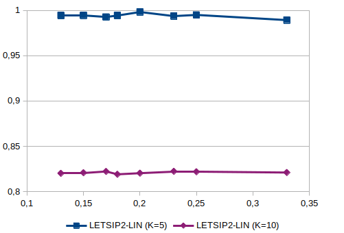
(a) LetSIP-disc-Lin: varying $k$, $\max.\varphi$

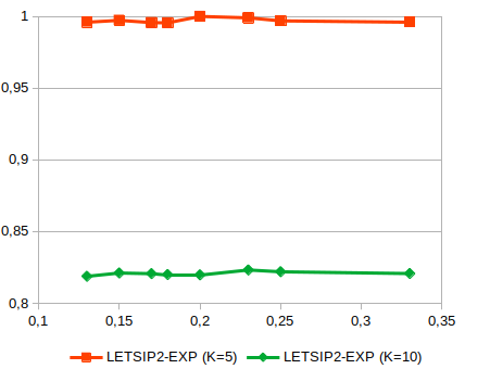
(b) LetSIP-disc-Exp: varying $k$, $\max.\varphi$

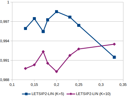
(c) LetSIP-disc-Lin: varying $k$, $Avg.\varphi$.

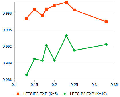
(d) LetSIP-disc-Exp: varying $k$, $Avg.\varphi$

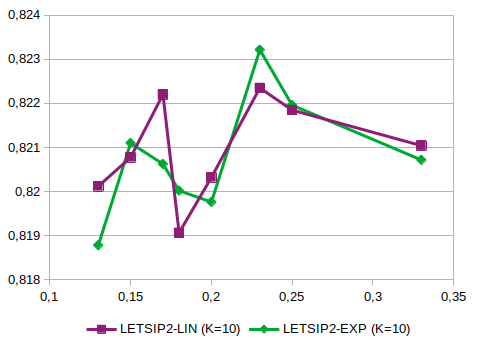
(e) Lin vs. Exp w.r.t. $\max.\varphi$.

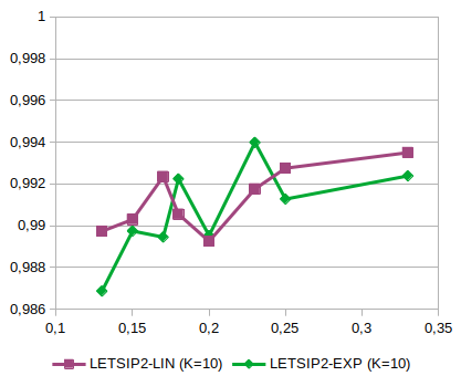
(f) Lin vs. Exp w.r.t. $Avg.\varphi$.

Figure 2: Effect of LetSIP-disc’s parameters on regret w.r.t. two performance measures ($\max.\varphi$ and $Avg.\varphi$) and query retention $\ell$ = 0. Results are aggregated over data sets and the three feature combinations I, IT and ILFT. Regret values are normalized to the range [0,1].

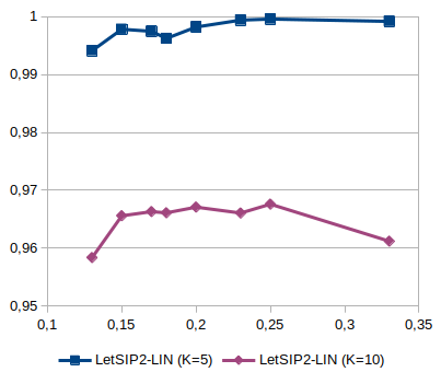
(a) LetSIP-disc-Lin: varying $k$, $\max~{}\varphi$.

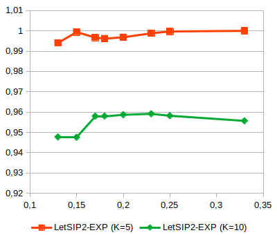
(b) LetSIP-disc-Exp: varying $k$, $\max~{}\varphi$

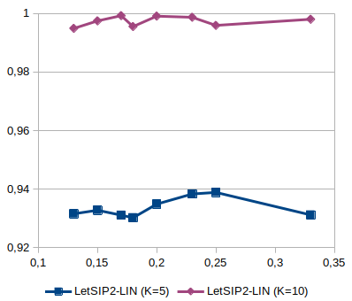
(c) LetSIP-disc-Lin: varying $k$ $Avg~{}\varphi$.

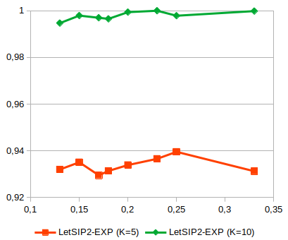
(d) LetSIP-disc-Exp: varying $k$ $Avg~{}\varphi$

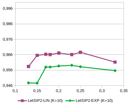
(e) Linvs. Expw.r.t. $\max.\varphi$.

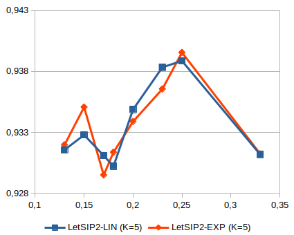
(f) Linvs. Expw.r.t. $Avg.\varphi$.

Figure 3: Effect of LetSIP-disc’s parameters on regret w.r.t. two performance measures ($\max.\varphi$ and $Avg.\varphi$) and query retention $\ell$ = 1. Results are aggregated over data sets and the three feature combinations I, IT and ILFT. Regret values are normalized to the range [0,1].

6.2 Experimental results

6.2.1 Evaluating Aspects of LetSIP-disc

In the first part of the experimental evaluation, we take a look at the effect of different parameter settings on LetSIP-disc, the influence of different pattern features, and how it compares to LetSIP itself.

Evaluating the influence of parameter settings We evaluate the effects of the choice of parameters values on the performance of LetSIP-disc, in particular query size $k\in\{5,10\}$, the aggregation function $\Phi$ and the range $\eta$. We use the following feature combination: $Items$ (I); $Items+Transactions$ (IT); and $Items+Length+Frequency+Transactions$ (ILFT). We consider two settings for parameter $\ell$: $\ell=0$ and $\ell=1$.

Figure 2 shows the effect of LetSIP-disc’s parameters on regret w.r.t. two performance measures ($\max.\varphi$ and $Avg.\varphi$) and query retention $\ell$ = 0. Figures 2a and 2b show that both aggregation functions ensure the lowest quality regrets with $k=10$ w.r.t. the $maximal$ aggregator. This indicates that our approach is able to identify the properties of the target ranking from ordered lists of patterns even when the query size increases. Additionally, the exponential function yields lower regret and $\eta=0.13$ seems the best value. Regarding the $average$ quality regret (see Figures 2c and 2d), $k=10$ continues to be the better query size for the exponential aggregation function but for the linear function, this depends on the value of $\eta$. In addition, as Figures 2e and 2f show, while the exponential function lead to lower maximal regret with $\eta=0.13$, the linear function can lead to lower average regret for higher values of $\eta$.

Figure 3 shows the effect of LetSIP-disc’s parameters on regret for query retention $\ell=1$. Retaining one highest-ranked pattern from the previous query w.r.t. $maximal$ quality does not affect the conclusions drawn previously: $k=10$ being the better query size and exponential function results in the lowest regret with $\eta=0.13$. However, we can see the opposite behaviour w.r.t. $average$ quality (see Figures 3c and 3d): querying $5$ patterns allows attaining low regret values for both functions, linear and exponential. Interestingly, as Figure 3e shows, the exponential function outperforms linear function on almost all values of $\eta$. Based on these findings, we use the following parameters in the next experiments: $k=10$, $aggregation$ = exponential and $\eta=0.13$.

Table 2: Evaluation of the importance of pattern features and comparison of LetSIP-disc-Exp ($\eta=0.13$) vs. LetSIP w.r.t. two performance measures. $k=10$. Results are aggregated over representative datasets: Anneal, Chess, German, Heart-cleveland, Hepatitis, Kr-vr-vp, Lymph, Mushroom, Soybean, Vote and Zoo-1.

	$\ell=0$ (fully random queries)					$\ell=1$ (retain $top$ $\ell$ patterns from the previous query)
	Regret: $\max.\varphi$		Regret: $Avg.\varphi$			Regret: $\max.\varphi$		Regret: $Avg.\varphi$
Features	LetSIP	LetSIP-disc-Exp	LetSIP	LetSIP-disc-Exp		LetSIP	LetSIP-disc-Exp	LetSIP	LetSIP-disc-Exp
I	269.419	271.434	617.328	615.994		196.655	200.975	574.396	575.46
IT	265.718	251.613	610.294	566.790		194.396	190.524	563.549	534.723
ITLF	263.067	249.577	605.779	561.667		196.161	193.554	568.200	534.129

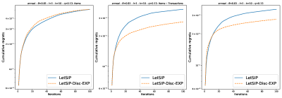
(a)

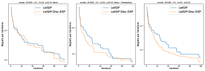
(b)

Figure 4: Anneal dataset: A detailed view of comparison between LetSIP-disc-Exp and LetSIP (cumulative and non-cumulative regret) for different pattern features w.r.t. $maximal$ quality, $k=10$ and $\ell=1$. Other results are reported in the Appendix A.

(a)

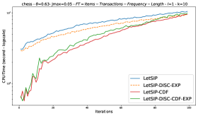
(b)

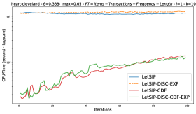
(c)

(d)

Figure 5: CPU-time analysis (sec.) of LetSIP, LetSIP-cdf, LetSIP-disc and LetSIP-disc-cdf-exp w.r.t. the ILFT feature combination. $k=10$ and $\ell=1$. Other results are reported in the Appendix C.

Table 3: Evaluation of the importance of pattern features and comparison of LetSIP-cdf vs. LetSIP w.r.t. different values of $J_{max}$. Results are aggregated over $11$ datasets : Lymph, Hepatitis, Heart-cleveland, Zoo-1, German-credit, Vote, Heart, Hypo, Soybean, Vehicle and Wine.

	$J_{max}=0.05\quad\wedge\quad\ell=1$
	$k=5$					$k=10$
	Regret: $\max.\varphi$		Regret: $Avg.\varphi$			Regret: $\max.\varphi$		Regret: $Avg.\varphi$
Features	LetSIP	LetSIP-cdf	LetSIP	LetSIP-cdf		LetSIP	LetSIP-cdf	LetSIP	LetSIP-cdf
I	204.595	13.860	424.472	337.069		196.444	10.986	433.142	376.380
IT	202.929	15.334	386.053	319.262		195.497	11.401	394.804	356.897
ITLF	206.064	15.517	383.799	320.838		197.422	11.521	393.147	356.395
	$J_{max}=0.05\quad\wedge\quad\ell=0$
	$k=5$					$k=10$
	Regret: $\max.\varphi$		Regret: $Avg.\varphi$			Regret: $\max.\varphi$		Regret: $Avg.\varphi$
Features	LetSIP	LetSIP-cdf	LetSIP	LetSIP-cdf		LetSIP	LetSIP-cdf	LetSIP	LetSIP-cdf
I	278.654	106.825	475.504	418.096		236.058	52.951	450.757	418.395
IT	264.425	103.516	428.160	392.522		235.397	53.939	414.606	395.671
ITLF	265.064	102.076	427.891	390.341		233.159	54.099	411.115	394.695
	$J_{max}=0.1\quad\wedge\quad\ell=1$
	$k=5$					$k=10$
	Regret: $\max.\varphi$		Regret: $Avg.\varphi$			Regret: $\max.\varphi$		Regret: $Avg.\varphi$
Features	LetSIP	LetSIP-cdf	LetSIP	LetSIP-cdf		LetSIP	LetSIP-cdf	LetSIP	LetSIP-cdf
I	204.595	8.647	424.472	348.129		196.444	4.360	433.142	386.818
IT	202.929	8.577	386.053	327.095		195.497	5.688	394.804	365.700
ITLF	206.064	8.514	383.799	327.133		197.422	5.595	393.147	366.117
	$J_{max}=0.1\quad\wedge\quad\ell=0$
	$k=5$					$k=10$
	Regret: $\max.\varphi$		Regret: $Avg.\varphi$			Regret: $\max.\varphi$		Regret: $Avg.\varphi$
Features	LetSIP	LetSIP-cdf	LetSIP	LetSIP-cdf		LetSIP	LetSIP-cdf	LetSIP	LetSIP-cdf
I	278.654	114.012	475.504	431.636		236.058	54.659	450.757	430.048
IT	264.425	96.029	428.160	406.527		235.397	43.409	414.606	408.651
ITLF	265.064	96.724	427.891	407.117		233.159	43.419	411.115	409.534

Table 4: Evaluation of the importance of pattern features and comparison of LetSIP-cdf vs. LetSIP w.r.t. different values of $J_{max}$. Results are aggregated over $4$ datasets : Kr-vs-kp, Chess, Mushroom and Anneal.

	$J_{max}=0.05\quad\wedge\quad\ell=1$
	$k=5$					$k=10$
	Regret: $\max.\varphi$		Regret: $Avg.\varphi$			Regret: $\max.\varphi$		Regret: $Avg.\varphi$
Features	LetSIP	LetSIP-cdf	LetSIP	LetSIP-cdf		LetSIP	LetSIP-cdf	LetSIP	LetSIP-cdf
I	4.846	277.351	153.230	338.841		2.052	276.587	173.482	346.336
IT	3.721	277.083	136.091	337.744		1.805	276.389	159.646	344.876
ITLF	3.813	277.083	139.184	337.744		1.765	276.395	165.982	344.702
	$J_{max}=0.05\quad\wedge\quad\ell=0$
	$k=5$					$k=10$
	Regret: $\max.\varphi$		Regret: $Avg.\varphi$			Regret: $\max.\varphi$		Regret: $Avg.\varphi$
Features	LetSIP	LetSIP-cdf	LetSIP	LetSIP-cdf		LetSIP	LetSIP-cdf	LetSIP	LetSIP-cdf
I	63.471	309.137	193.516	353.573		34.480	291.099	192.332	353.918
IT	52.438	307.783	179.867	352.255		28.021	291.124	184.793	352.418
ITLF	52.554	307.707	179.214	352.238		27.751	290.265	183.861	351.850
	$J_{max}=0.1\quad\wedge\quad\ell=1$
	$k=5$					$k=10$
	Regret: $\max.\varphi$		Regret: $Avg.\varphi$			Regret: $\max.\varphi$		Regret: $Avg.\varphi$
Features	LetSIP	LetSIP-cdf	LetSIP	LetSIP-cdf		LetSIP	LetSIP-cdf	LetSIP	LetSIP-cdf
I	4.846	277.948	153.230	338.357		2.052	276.515	173.482	345.652
IT	3.721	277.414	136.091	336.254		1.805	276.432	159.646	344.235
ITLF	3.813	277.412	139.184	336.137		1.765	276.426	165.982	344.243
	$J_{max}=0.1\quad\wedge\quad\ell=0$
	$k=5$					$k=10$
	Regret: $\max.\varphi$		Regret: $Avg.\varphi$			Regret: $\max.\varphi$		Regret: $Avg.\varphi$
Features	LetSIP	LetSIP-cdf	LetSIP	LetSIP-cdf		LetSIP	LetSIP-cdf	LetSIP	LetSIP-cdf
I	63.471	309.973	193.516	353.422		34.480	291.349	192.332	353.411
IT	52.438	305.787	179.867	352.103		28.021	290.251	184.793	352.371
ITLF	52.554	306.007	179.214	352.039		27.751	290.893	183.861	352.192

Evaluating the importance of pattern features. In order to evaluate the importance of various feature sets we performed the following procedure. We construct feature representations of patterns incrementally, i.e. we start with an empty representation and add feature sets one by one, based on the improvement of learning accurate pattern rankings that they enable. Table 2 shows the results for two settings of query retention $\ell$. As we can observe, additional features provide valuable information to learn more accurate pattern rankings, particularly for LetSIP-disc-Exp where the regret values all decrease. These results are consistent with those observed in Dzyuba:letsip . However, the importance of features depends on the pattern type and the target measure $\varphi$ DzyubaLNR14 . For surprising pattern mining, $Length$ is the most likely to be included in the best feature set, because long patterns tend to have higher values of Surprisingness. $Items$ are important as well, because individual item frequencies are directly included in the formula of Surprisingness. $Transactions$ are important because this feature set helps capture interactions between other features, albeit indirectly.

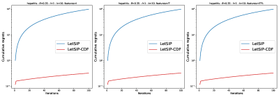
(a)

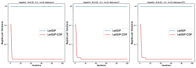
(b)

Figure 6: Hepatitis dataset: A detailed view of comparison between LetSIP-cdf and LetSIP (cumulative and non-cumulative regret) for different pattern features w.r.t. $maximal$ quality, $k=10$ and $\ell=1$. Other results are reported in the Appendix B.

Comparing quality regrets of LetSIP-disc with LetSIP. Dzyuba:letsip showed that LetSIP outperforms two state-of-the-art interactive methods, APLe DzyubaLNR14 , another approach based on active preference learning to learn a linear ranking function using RankSVM, and IPM DBLP:journals/sadm/BhuiyanH16 , an MCMC-based interactive sampling framework. Thus, we compare LetSIP-disc-Exp with LetSIP. We use query size $k$ and feature representations identical to LetSIP-disc-Exp and we vary the query retention $\ell$. Table 2 reports the regret values. When considering $Items$ as feature representation for patterns, LetSIP performs the best w.r.t. $maximal$ quality. However, selecting queries uniformly at random allows LetSIP-disc-Exp to ensure the lowest quality regrets w.r.t. $average$ quality. Regarding the other features (IT and ITLF), LetSIP-disc-Exp always outperforms LetSIP whatever the value of the query retention $\ell$ and the performance measure considered. On the other hand, we observe that the improvements are more pronounced w.r.t. $average$ regret. These results indicate that the learned ranks by LetSIP-disc of the $k$ selected patterns of each query in the target ranking are more accurate compared to those learned by LetSIP; average values of surprisingness increase substantially compared to LetSIP rankings.

Finally, retaining one highest-ranked pattern ($\ell=1$) results in the lowest regret whatever the feature representations of patterns. As explained in Dzyuba:letsip , fully random queries ($\ell=0$) do not enable sufficient exploitation for learning accurate weights.

Figure 4 presents a detailed view of the comparison between LetSIP-disc-cdf-exp and LetSIP on Anneal dataset (other results are given in the Appendix A). Curves show the evolution of the regret (cumulative and non cumulative) in the resulting frequent patterns over $100$ iterations of learning. The results confirm that the learned ranking function of LetSIP-disc-Exp have the capacity to identify frequent patterns with higher quality (i.e., of lowest regrets).

CPU-times analysis. Finally, regarding the CPU-times, Figure 5 compares the performance of LetSIP-disc-Exp and LetSIP on German-credit, Chess, Heart-Cleveland and Zoo-1 datasets. Overall, learning more complex descriptors from the user-defined pattern ranking does not add significantly to the runtimes of our approach. LetSIP-disc-Exp clearly beats LetSIP on four datasets (i.e., Chess, Heart-cleveland, Kr-vs-kp, and Soybean) and performs similarly on three other ones (see complementary results in the Appendix C), while LetSIP performs better on three datasets (i.e., German-credit, Hepatitis, Zoo).

On average, one iteration of LetSIP-disc-Exp takes 8.84s (8.81s for LetSIP) on AMD Opteron 6174 with 2.2 GHz. The largest proportion of LetSIP’s runtime costs is associated with the sampling component (costs of weight learning are low). As it will be shown in the next Section, exploiting cdFlexics within LetSIP enables to improve the running times.

6.2.2 Evaluating Aspects of LetSIP-cdf

We investigate the effects of the choice of features and parameter values on the performance of LetSIP-cdf and we compare it to the original LetSIP. We use the same protocol as in Section 6.2.1. We consider two settings for parameter $J_{max}\in\{0.05,0.1\}$. Tables 3 and 4 show detailed results.

As observed previously, in almost of the cases, adding new features allow to decrease the value of the regret. Interestingly, increasing the query size decreases the maximal quality regret about twofold, while for the average quality regret $k=5$ seems to be the best setting. Regarding the parameter $J_{max}$, the performance depends on the target measure $\varphi$: $J_{max}=0.1$ results in the lowest regret with respect to the $maximal$ quality, while $J_{max}=0.05$ ensures the lowest $average$ quality regrets. Finally, for the choice of values for query retention $\ell$, we observe the same conclusions drawn previously: $\ell=1$ being the better query retention value.

Comparing quality regrets of LetSIP-cdf with LetSIP. LetSIP-cdf exhibits two different behaviours. On $11$ datasets (see Table 3), the regret of LetSIP-cdf is substantially lower than that of LetSIP, particularly for the $maximal$ quality and for $\ell=1$ where the decrease is very impressive (an average gain of $94\%$). However, it is also results in the highest quality regrets on four datasets (see Table 4), which negates the previous results.

An analysis of the results on these four data sets shows us that closedDiversity mines very few patterns for each query. This is due to the use of a rather low diversity threshold ($J_{max}$ =0.05) which considerably reduces the many redundancies in these data sets. The trade-off is, however, that it becomes extremely difficult to improve the regret given the few patterns.

Figure 6 presents a detailed view of the comparison between LetSIP-cdf and LetSIP (cumulative and non-cumulative regret) on Hepatitis dataset (other results are given in the Appendix B). These results confirm once again the interest of ensuring higher diversity for learning accurate weights.

CPU-times analysis. Figure 5 also compares the performance of LetSIP-cdf and LetSIP on German-credit, Chess, Heart-Cleveland and Zoo-1 data sets. Other results are given in the Appendix C. Clearly, LetSIP-cdf is more efficient than LetSIP. This is explainable by the large reduction of the size of each cell performed by closedDiversity to avoid the mining of non diverse patterns, which speeds exploration up. The only exception are the two data sets Zoo-1 and Vote where LetSIP is faster. When comparing to LetSIP-disc-cdf-exp, we can observe that LetSIP-cdf remains better, except again for the two data sets Zoo-1 and Vote.

6.2.3 Evaluating Aspects of LetSIP-disc-cdf

Our last experiments evaluates the combination of our two improvements to LetSIP, i.e., the improved sampling of cdFlexics and the more complex features learned dynamically during the iterative mining process. We report detailed results for different features combination, and different parameter settings (query size $k$, query retention $\ell$, and $\eta$). We only show the results for $J_{max}=0.05$. As previously, LetSIP-disc-cdf clearly beats LetSIP-cdf on $11$ datasets (see Tables 5) whatever the feature representations of patterns and the value of parameters $k$ and $\eta$. When comparing to LetSIP-cdf, the choice of values for query retention $\ell$ clearly affects LetSIP-disc-cdf. Fully random queries ($\ell=0$) seems to favour LetSIP-disc-cdf, yielding small improvements. However, both aggregation functions EXP and Linear get similar results with a slight advantage for EXP. The results of LetSIP-disc-cdf with $\ell=1$ are comparable with those of LetSIP-cdf, but we can notice a very slight advantage to LetSIP-disc-cdf with ILFT as feature representation for patterns. As for LetSIP-cdf, LetSIP-disc-cdf performs badly on four datasets (see Table 5).

CPU-times analysis. When analysing the running times (see Figure 5), we can see that LetSIP-cdf and LetSIP-disc-cdf perform very similarly on most of the instances, except on two datasets (Kr-vr-kp and Zoo-1) where LetSIP-disc-cdf is faster.

Table 5: Evaluation of the importance of pattern features and comparison of LetSIP-disc-cdfvs LetSIP-cdf vs. LetSIP w.r.t. different values of $J_{max}$. Results are aggregated over $11$ datasets : Lymph, Hepatitis, Heart-cleveland, Zoo, German-credit, Soybean, Vote, Heart, Hypo, Vehicle and Wine.

		$J_{max}=0.05\quad\wedge\quad\ell=1$
		$k=5$										$k=10$
		Regret: $\max.\varphi$					Regret: $Avg.\varphi$					Regret: $\max.\varphi$					Regret: $Avg.\varphi$
Features	$\eta$	LetSIP	LetSIP-cdf	LetSIP-disc-cdf			LetSIP	LetSIP-cdf	LetSIP-disc-cdf			LetSIP	LetSIP-cdf	LetSIP-disc-cdf			LetSIP	LetSIP-cdf	LetSIP-disc-cdf
				EXP	Linear				EXP	Linear				EXP	Linear				EXP	Linear
I	0.25	204.595	13.860	13.934	13.806		424.472	337.069	341.575	340.623		196.444	10.986	11.127	11.167		433.142	376.380	378.948	378.690
	0.2			14.018	14.017				340.322	341.283				11.229	11.122				379.438	379.070
	0.13			13.957	13.982				339.773	340.131				11.195	11.283				377.142	377.700
IT	0.25	202.929	15.334	15.533	15.424		386.053	319.262	320.589	320.195		195.497	11.401	11.654	11.660		394.804	356.897	358.164	357.460
	0.2			15.857	15.798				320.975	321.036				11.596	11.510				357.211	357.257
	0.13			15.698	15.404				319.366	318.690				11.694	11.678				358.401	358.065
ITLF	0.25	206.064	15.517	15.552	15.539		383.799	320.838	320.572	320.792		197.422	11.521	11.478	11.475		393.147	356.395	359.163	357.518
	0.2			15.373	15.568				319.694	320.782				11.562	11.577				358.267	357.770
	0.13			15.504	15.432				320.250	320.435				11.568	11.603				357.917	358.845
		$J_{max}=0.05\quad\wedge\quad\ell=0$
		$k=5$										$k=10$
		Regret: $\max.\varphi$					Regret: $Avg.\varphi$					Regret: $\max.\varphi$					Regret: $Avg.\varphi$
Features	$\eta$	LetSIP	LetSIP-cdf	LetSIP-disc-cdf			LetSIP	LetSIP-cdf	LetSIP-disc-cdf			LetSIP	LetSIP-cdf	LetSIP-disc-cdf			LetSIP	LetSIP-cdf	LetSIP-disc-cdf
				EXP	Linear				EXP	Linear				EXP	Linear				EXP	Linear
I	0.25	278.654	106.825	106.584	107.366		475.504	418.096	420.378	421.057		236.058	52.951	52.131	52.678		450.757	418.395	419.840	420.121
	0.2			106.865	105.939				420.432	419.443				52.811	53.053				419.507	420.455
	0.13			106.378	106.834				418.817	419.686				52.768	52.980				419.344	419.514
IT	0.25	264.425	103.516	102.476	102.641		428.160	392.522	389.494	390.337		235.397	53.939	54.234	54.072		414.606	395.671	394.871	395.244
	0.2			100.760	100.996				388.681	388.808				53.874	53.459				395.652	395.075
	0.13			102.946	101.420				391.117	390.838				53.466	53.450				395.346	394.423
ITLF	0.25	265.064	102.076	102.838	102.197		427.891		391.805	391.119		233.159	54.099	54.004	54.271		411.115	394.695	395.034	396.046
	0.2			101.825	102.152			390.341	389.838	390.432				53.599	53.312				394.887	394.219
	0.13			101.531	101.638				388.785	390.178				53.764	53.730				394.854	395.121

Table 6: Evaluation of the importance of pattern features and comparison of LetSIP-disc-cdfvs LetSIP-cdf vs. LetSIP w.r.t. different values of $J_{max}$. Results are aggregated over $4$ datasets : Kr-vs-kp, Chess, Mushroom and Anneal.

		$J_{max}=0.05\quad\wedge\quad\ell=1$
		$k=5$										$k=10$
		Regret: $\max.\varphi$					Regret: $Avg.\varphi$					Regret: $\max.\varphi$					Regret: $Avg.\varphi$
Features	$\eta$	LetSIP	LetSIP-cdf	LetSIP-disc-cdf			LetSIP	LetSIP-cdf	LetSIP-disc-cdf			LetSIP	LetSIP-cdf	LetSIP-disc-cdf			LetSIP	LetSIP-cdf	LetSIP-disc-cdf
				EXP	Linear				EXP	Linear				EXP	Linear				EXP	Linear
I	0.25	4.846	277.351	277.369	277.369		153.230	338.841	339.439	339.293		2.052	276.587	276.624	276.626		173.482	346.336	346.241	346.167
	0.2			277.289	277.289				338.776	338.635				276.653	276.653				346.442	346.521
	0.13			277.296	277.296				338.963	339.004				276.767	276.767				346.311	346.296
IT	0.25	3.721	277.083	277.114	277.114		136.091	337.744	337.976	337.976		1.805	276.389	276.599	276.599		159.646	344.876	344.324	344.294
	0.2			277.116	277.113				337.834	337.756				276.559	276.559				344.605	344.690
	0.13			277.116	277.116				338.160	338.160				276.593	276.593				344.557	344.550
ITLF	0.25	3.813	277.083	277.114	277.114		139.184	337.744	338.259	337.976		1.765	276.395	276.596	276.596		165.982	344.702	344.479	344.454
	0.2			277.116	277.116				337.834	337.834				276.560	276.559				344.497	344.646
	0.13			277.116	277.115				338.160	338.078				276.594	276.594				344.409	344.409
		$J_{max}=0.05\quad\wedge\quad\ell=0$
		$k=5$										$k=10$
		Regret: $\max.\varphi$					Regret: $Avg.\varphi$					Regret: $\max.\varphi$					Regret: $Avg.\varphi$
Features	$\eta$	LetSIP	LetSIP-cdf	LetSIP-disc-cdf			LetSIP	LetSIP-cdf	LetSIP-disc-cdf			LetSIP	LetSIP-cdf	LetSIP-disc-cdf			LetSIP	LetSIP-cdf	LetSIP-disc-cdf
				EXP	Linear				EXP	Linear				EXP	Linear				EXP	Linear
I	0.25	63.471	309.137	310.595	311.030		193.516	353.573	354.350	354.350		34.480	291.099	291.640	291.393		192.332	353.918	353.919	353.938
	0.2			311.746	311.736				354.446	354.463				290.972	290.637				353.659	353.396
	0.13			308.817	308.978				353.450	353.482				291.020	290.889				353.562	353.507
IT	0.25	52.438	307.783	308.256	308.041		179.867	352.255	352.338	352.426		28.021	291.124	291.428	291.454		184.793	352.418	352.716	352.693
	0.2			308.661	308.294				352.516	352.405				290.208	290.646				352.482	352.413
	0.13			307.111	307.111		179.867	352.255	351.959	351.959				290.909	290.909				352.092	352.092
ITLF	0.25	52.554	307.707	308.256	308.256		179.214	352.238	352.338	352.338		27.751	290.265	291.221	291.277		183.861	351.850	352.578	352.582
	0.2			308.453	308.453				352.395	352.395				290.300	290.319				352.342	352.352
	0.13			307.111	307.111				351.959	351.959				290.700	290.700				352.057	352.057

7 Related Work

Pattern mining has been faced with the problem of returning too large, and potentially uninteresting result sets since early on.

The first proposed solution consisted of condensed representations Lakhal ; DBLP:conf/ideas/2001:free ; DBLP:conf/pkdd/2002:non-derivable by reducing the redudancy of the covers of patterns. Top-$k$ mining morishita ; WangHLT05 is efficient but results in strongly related, redundant patterns showing a lack of diversity. Pattern set mining chosen-few ; DBLP:conf/kdd/2006:miki ; patternteams ; DBLP:conf/sdm/RaedtZ07 takes into account the relationships between the patterns, which allows to control redundancy and lead to small sets. It requires that one mines an ideally large pattern set to select from, and typically doesn’t involve the user.

Constraint-based pattern mining has been leveraged as a general, flexible solution to pattern mining for a while DBLP:conf/kdd/RaedtGN08 ; schaus2017coversize , and has since seen numerous improvements, including closed itemset mining lazaar2016global and, eventually mining of diverse itemsets HienLALLOZ20 .

The most recent proposal to dealing with the question of finding interesting patterns involves the user, via interactive pattern mining DBLP:conf/icml/Rueping09 often involving sampling DBLP:journals/sadm/BhuiyanH16 , with LetSIP Dzyuba:letsip one of the end points of this development.

8 Conclusion

In this paper, we have proposed an improvement to the state-of-the art of iterative pattern mining: instead of using static low-level features that have been pre-defined before the process starts, our approach learns more complex descriptors from the user-defined pattern ranking. These features allow to capture the importance of item interactions, and, as shown experimentally, lead to lower cumulative and individual regret than using low-level features. We have explored two multiplicative aggregation functions for mapping weights learned for complex features back to their component items, and find that the exponential multiplicative factor gives better results on most of the data sets we worked with. Furthermore, we have proposed to use cdFlexics as the sampling component in LetSIP to maximize the pattern diversity of each query and showed a straightforward combination of both improvements in LetSIP. cdFlexics takes the XOR-constraint based data partitioning of Flexics and extends it with the diversity constraint closedDiversity, introduced in HienLALLOZ20 . The results show convincing improvements both in terms of learning more accurate pattern rankings and CPU-times. We have evaluated our proposal only on itemset data so far since the majority of existing work, including the method that we extended, is defined for this kind of data. But the importance of using complex dynamic features can be expected to be even higher when interactively mining complex, i.e. sequential, tree-, or graph-structured data. We will explore this direction in future work.

Declarations

• Conflict of interest/Competing interests: all authors declare not having any financial or non-financial interests that are directly or indirectly related to the work submitted for publication.

• Availability of data, materials and code: They will be available in the final submission.

Appendix A Detailed view of results for other datasets (LetSIP-disc vs. LetSIP)

Figures 7-11 plot a detailed view of comparison between LetSIP-disc-Exp and LetSIP (cumulative and non-cumulative regret) for different datasets w.r.t. $maximal$ quality, $k=10$ and $\ell=1$.

(a)

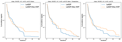
(b)

(c)

(d)

Figure 7: A detailed view of comparison between LetSIP-disc-Exp and LetSIP (cumulative and non-cumulative regret) for different pattern features w.r.t. $maximal$ quality, $k=10$ and $\ell=1$.

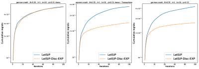
(a)

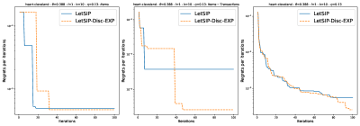
(b)

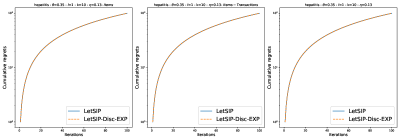
(c)

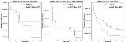
(d)

Figure 8: A detailed view of comparison between LetSIP-disc-Exp and LetSIP (cumulative and non-cumulative regret) for different pattern features w.r.t. $maximal$ quality, $k=10$ and $\ell=1$.

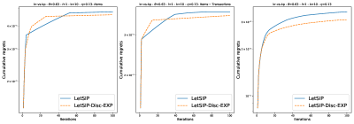
(a)

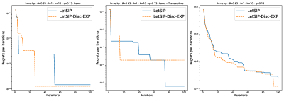
(b)

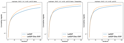
(c)

(d)

Figure 9: A detailed view of comparison between LetSIP-disc-Exp and LetSIP (cumulative and non-cumulative regret) for different pattern features w.r.t. $maximal$ quality, $k=10$ and $\ell=1$.

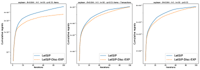
(a)

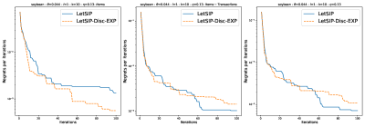
(b)

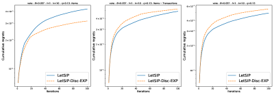
(c)

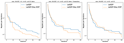
(d)

Figure 10: A detailed view of comparison between LetSIP-disc-Exp and LetSIP (cumulative and non-cumulative regret) for different pattern features w.r.t. $maximal$ quality, $k=10$ and $\ell=1$.

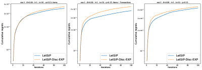
(a)

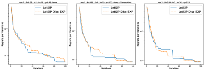
(b)

Figure 11: A detailed view of comparison between LetSIP-disc-Exp and LetSIP (cumulative and non-cumulative regret) for different pattern features w.r.t. $maximal$ quality, $k=10$ and $\ell=1$.

Appendix B Detailed view of results for other datasets (LetSIP-cdf vs. LetSIP)

Figures 12-15 plot a detailed view of comparison between LetSIP-cdf and LetSIP (cumulative and non-cumulative regret) for different datasets w.r.t. $maximal$ quality, $k=10$ and $\ell=1$.

(a)

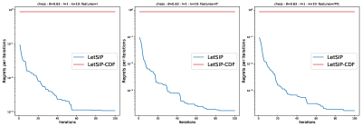
(b)

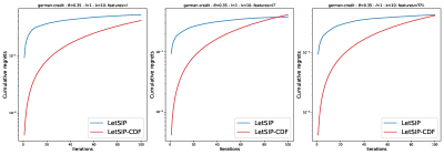
(c)

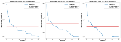
(d)

Figure 12: A detailed view of comparison between LetSIP-cdf and LetSIP (cumulative and non-cumulative regret) for different pattern features w.r.t. $maximal$ quality, $k=10$ and $\ell=1$.

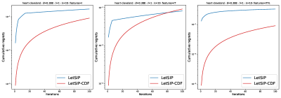
(a)

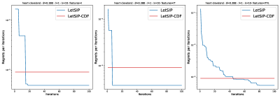
(b)

(c)

(d)

Figure 13: A detailed view of of comparison between LetSIP-cdf and LetSIP (cumulative and non-cumulative regret) for different pattern features w.r.t. $maximal$ quality, $k=10$ and $\ell=1$.

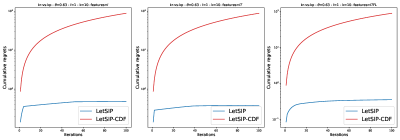
(a)

(b)

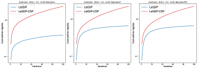
(c)

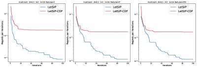
(d)

Figure 14: A detailed view of of comparison between LetSIP-cdf and LetSIP (cumulative and non-cumulative regret) for different pattern features w.r.t. $maximal$ quality, $k=10$ and $\ell=1$.

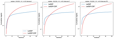
(a)

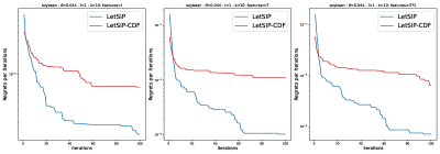
(b)

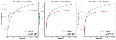
(c)

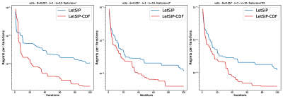
(d)

Figure 15: A detailed view of of comparison between LetSIP-cdf and LetSIP (cumulative and non-cumulative regret) for different pattern features w.r.t. $maximal$ quality, $k=10$ and $\ell=1$.

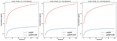
(a)

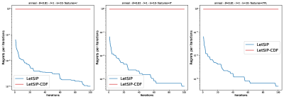
(b)

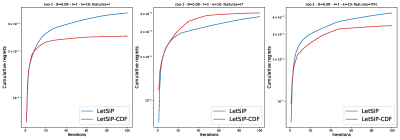
(c)

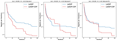
(d)

Figure 16: A detailed view of comparison between LetSIP-cdf and LetSIP and LetSIP (cumulative and non-cumulative regret) for different pattern features w.r.t. $maximal$ quality, $k=10$ and $\ell=1$.

Appendix C Complementary results for CPU-times comparison

Figure 17 compares the CPU-times of LetSIP, LetSIP-cdf, LetSIP-disc-Exp and LetSIP-disc-cdfw.r.t. the ILFT feature combination, $k=10$ and $\ell=1$.

	i

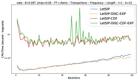
(a)

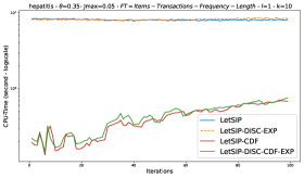
(b)

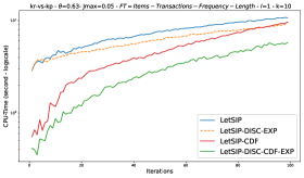
(c)

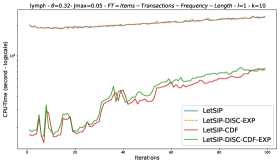
(d)

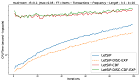
(e)

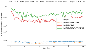
(f)

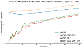
(g)

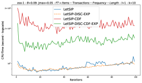
(h)

Figure 17: CPU-time analysis (sec.) of LetSIP, LetSIP-cdf, LetSIP-disc and LetSIP-disc-cdf-exp w.r.t. the ILFT feature combination. $k=10$ and $\ell=1$.

References

- \bibcommenthead
- (1) Agrawal, R., Srikant, R.: Fast algorithms for mining association rules in large databases. In: Proceedings of the 20th International Conference on Very Large Data Bases. VLDB ’94, pp. 487–499. Morgan Kaufmann Publishers Inc., Santiago de Chile, Chile (1994)
- (2) Tan, P.-N., Kumar, V., Srivastava, J.: Selecting the right interestingness measure for association patterns. In: KDD, pp. 32–41 (2002)
- (3) Pasquier, N., Bastide, Y., Taouil, R., Lakhal, L.: Discovering frequent closed itemsets for association rules. In: ICDT, vol. 1540, pp. 398–416 (1999)
- (4) De Raedt, L., Zimmermann, A.: Constraint-based pattern set mining. (2007)
- (5) Rüping, S.: Ranking interesting subgroups. In: Danyluk, A.P., Bottou, L., Littman, M.L. (eds.) Proceedings of the 26th Annual International Conference on Machine Learning, ICML 2009, Montreal, Quebec, Canada, June 14-18, 2009. ACM International Conference Proceeding Series, vol. 382, pp. 913–920 (2009). https://doi.org/10.1145/1553374.1553491. https://doi.org/10.1145/1553374.1553491
- (6) Dzyuba, V., van Leeuwen, M.: Learning what matters - sampling interesting patterns. In: PAKDD 2017, Proceedings, Part I, pp. 534–546 (2017)
- (7) Bhuiyan, M., Hasan, M.A.: Interactive knowledge discovery from hidden data through sampling of frequent patterns. Stat. Anal. Data Min. 9(4), 205–229 (2016)
- (8) Dzyuba, V., van Leeuwen, M., Raedt, L.D.: Flexible constrained sampling with guarantees for pattern mining. Data Min. Knowl. Discov. 31(5), 1266–1293 (2017)
- (9) Hoeve, W., Katriel, I.: Global constraints. In: Handbook of Constraint Programming, pp. 169–208 (2006)
- (10) Belaid, M., Bessiere, C., Lazaar, N.: Constraint programming for mining borders of frequent itemsets. In: Kraus, S. (ed.) Proceedings of the Twenty-Eighth International Joint Conference on Artificial Intelligence, IJCAI 2019, Macao, China, August 10-16, 2019, pp. 1064–1070 (2019)
- (11) Lazaar, N., Lebbah, Y., Loudni, S., Maamar, M., Lemière, V., Bessiere, C., Boizumault, P.: A global constraint for closed frequent pattern mining. In: Rueher, M. (ed.) Principles and Practice of Constraint Programming - 22nd International Conference, CP 2016, Toulouse, France, September 5-9, 2016, Proceedings. Lecture Notes in Computer Science, vol. 9892, pp. 333–349 (2016)
- (12) Raedt, L.D., Guns, T., Nijssen, S.: Constraint programming for itemset mining. In: Proceedings of the 14th ACM SIGKDD 2008, pp. 204–212 (2008)
- (13) Schaus, P., Aoga, J.O.R., Guns, T.: Coversize: A global constraint for frequency-based itemset mining. In: Proceedings of the 23rd CP 2017, pp. 529–546 (2017)
- (14) Khiari, M., Boizumault, P., Crémilleux, B.: Constraint programming for mining n-ary patterns. In: Cohen, D. (ed.) Principles and Practice of Constraint Programming - CP 2010 - 16th International Conference, CP 2010, St. Andrews, Scotland, UK, September 6-10, 2010. Proceedings. Lecture Notes in Computer Science, vol. 6308, pp. 552–567 (2010)
- (15) Hien, A., Loudni, S., Aribi, N., Lebbah, Y., Laghzaoui, M.E.A., Ouali, A., Zimmermann, A.: A relaxation-based approach for mining diverse closed patterns. In: Hutter, F., Kersting, K., Lijffijt, J., Valera, I. (eds.) Machine Learning and Knowledge Discovery in Databases - European Conference, ECML PKDD 2020, Ghent, Belgium, September 14-18, 2020, Proceedings, Part I. Lecture Notes in Computer Science, vol. 12457, pp. 36–54 (2020). https://doi.org/10.1007/978-3-030-67658-2_3. https://doi.org/10.1007/978-3-030-67658-2_3
- (16) Meel, K.S., Vardi, M.Y., Chakraborty, S., Fremont, D.J., Seshia, S.A., Fried, D., Ivrii, A., Malik, S.: Constrained sampling and counting: Universal hashing meets SAT solving. In: Beyond NP, Papers from the 2016 AAAI Workshop, 2016 (2016)
- (17) Chakraborty, S., Fremont, D.J., Meel, K.S., Seshia, S.A., Vardi, M.Y.: Distribution-aware sampling and weighted model counting for SAT. CoRR abs/1404.2984 (2014)
- (18) Gomes, C.P., van Hoeve, W.J., Sabharwal, A., Selman, B.: Counting CSP solutions using generalized XOR constraints. In: Proceedings of the Twenty-Second AAAI Conference on Artificial Intelligence, July 22-26, 2007, Vancouver, British Columbia, Canada, pp. 204–209 (2007). http://www.aaai.org/Library/AAAI/2007/aaai07-031.php
- (19) Morishita, S., Sese, J.: Traversing itemset lattices with statistical metric pruning. In: Proceedings of the Nineteenth ACM SIGACT-SIGMOD-SIGART Symposium, pp. 226–236 (2000)
- (20) Arora, S., Hazan, E., Kale, S.: The multiplicative weights update method: a meta-algorithm and applications. Theory Comput. 8(1), 121–164 (2012)
- (21) Dzyuba, V., van Leeuwen, M., Nijssen, S., Raedt, L.D.: Interactive learning of pattern rankings. International Journal on Artificial Intelligence Tools 23(6) (2014)
- (22) Boulicaut, J.-F., Jeudy, B.: Mining free itemsets under constraints. In: Proceedings 2001 International Database Engineering and Applications Symposium, pp. 322–329 (2001). https://doi.org/10.1109/IDEAS.2001.938100
- (23) Calders, T., Goethals, B.: Mining all non-derivable frequent itemsets. In: Proceedings of the 6th European Conference on Principles of Data Mining and Knowledge Discovery. PKDD ’02, pp. 74–85 (2002)
- (24) Wang, J., Han, J., Lu, Y., Tzvetkov, P.: TFP: an efficient algorithm for mining top-k frequent closed itemsets. IEEE Trans. Knowl. Data Eng. 17(5), 652–664 (2005)
- (25) Bringmann, B., Zimmermann, A.: The chosen few: On identifying valuable patterns. In: Proceedings of the 7th IEEE International Conference on Data Mining (ICDM 2007), October 28-31, 2007, Omaha, Nebraska, USA, pp. 63–72 (2007). https://doi.org/10.1109/ICDM.2007.85. https://doi.org/10.1109/ICDM.2007.85
- (26) Knobbe, A.J., Ho, E.K.Y.: Maximally informative k-itemsets and their efficient discovery. In: KDD ’06, pp. 237–244 (2006)
- (27) Knobbe, A.J., Ho, E.K.Y.: Pattern teams. In: Proceedings of the 10th European Conference on Principles and Practice of Knowledge Discovery in Databases. ECMLPKDD’06, pp. 577–584. Springer, Berlin, Heidelberg (2006)
- (28) Raedt, L.D., Guns, T., Nijssen, S.: Constraint programming for itemset mining. In: Li, Y., Liu, B., Sarawagi, S. (eds.) Proceedings of the 14th ACM SIGKDD International Conference on Knowledge Discovery and Data Mining, Las Vegas, Nevada, USA, August 24-27, 2008, pp. 204–212 (2008). https://doi.org/10.1145/1401890.1401919. https://doi.org/10.1145/1401890.1401919
- (29) Schaus, P., Aoga, J.O., Guns, T.: Coversize: A global constraint for frequency-based itemset mining. In: International Conference on Principles and Practice of Constraint Programming, pp. 529–546 (2017). Springer
- (30) Bhuiyan, M., Hasan, M.A.: Interactive knowledge discovery from hidden data through sampling of frequent patterns. Stat. Anal. Data Min. 9(4), 205–229 (2016). https://doi.org/10.1002/sam.11322
- (31) Lazaar, N., Lebbah, Y., Loudni, S., Maamar, M., Lemière, V., Bessiere, C., Boizumault, P.: A global constraint for closed frequent pattern mining. In: International Conference on Principles and Practice of Constraint Programming, pp. 333–349 (2016). Springer