Mantle Degassing Lifetimes through Galactic Time and the Maximum Age Stagnant-lid Rocky Exoplanets can Support Temperate Climates
Abstract
The ideal exoplanets to search for life are those within a star’s habitable zone. However, even within the habitable zone planets can still develop uninhabitable climate states. Sustaining a temperate climate over geologic (Gyr) timescales requires a planet contain sufficient internal energy to power a planetary-scale carbon cycle. A major component of a rocky planet’s energy budget is the heat produced by the decay of radioactive elements, especially 40K, 232Th, 235U and 238U. As the planet ages and these elements decay, this radiogenic energy source dwindles. Here we estimate the probability distribution of the amount of these heat producing elements (HPEs) that enter into rocky exoplanets through Galactic history, by combining the system-to-system variation seen in stellar abundance data with the results from Galactic chemical evolution models. Using these distributions, we perform Monte-Carlo thermal evolution models that maximize the mantle cooling rate. This allows us to create a pessimistic estimate of lifetime a rocky, stagnant-lid exoplanet can support a global carbon cycle and temperate climate as a function of its mass and when it in Galactic history. We apply this framework to a sample of 17 likely rocky exoplanets with measured ages, 7 of which we predict are likely to be actively degassing today despite our pessimistic assumptions. For the remaining planets, including those orbiting TRAPPIST-1, we cannot confidently assume they currently contain sufficient internal heat to support mantle degassing at a rate sufficient to sustain a global carbon cycle or temperate climate without additional tidal heating or undergoing plate tectonics.
1 Introduction
The climate state of an exoplanet is a primary determining factor of whether it is likely to be habitable to life as we know it. While life may manifest within subglacial oceans such as those on icy moons, surface life is more easily detected remotely. Thus, a temperate surface is often considered a first-order requirement for detectable life to develop on a planet. The likelihood of a temperate climate is typically assessed based on the stellar radiation a planet receives, particularly whether it lies within its host-star’s so-called “habitable zone” (e.g., Kasting et al., 1993; Kopparapu et al., 2013). Lying within a star’s habitable zone, however, does not guarantee that a planet will have a temperate surface suitable for liquid water or life. Indeed, to truly be considered habitable, a planet must be neither too hot to evaporate the entirety of its water nor sterilize the planet’s surface (e.g., Abbot et al., 2012; Foley & Driscoll, 2016), or too cold to undergo global glaciation (Kadoya & Tajika, 2014; Menou, 2015; Haqq-Misra et al., 2016); both extremes can develop even within the nominal habitable zone.
Whether a planet is capable of consistently remaining in this temperate state over geologic (Gyr) timescales relies, in part, on its ability to regulate the abundance of greenhouse gases in its atmosphere. Of the major greenhouse gases, CO2 is known to be regulated by the carbonate-silicate cycle, at least on Earth. The balance between the rate of delivery of CO2 to the atmosphere via melt-induced degassing of carbon in the mantle or crust, weathering and return of C in the form of carbonates to the mantle determines atmospheric CO2 concentrations; negative feedbacks involved in surface weathering and degassing help to stabilize climate (e.g., Walker et al., 1981; Sleep & Zahnle, 2001; Kasting & Catling, 2003; Foley & Driscoll, 2016). However, this stabilizing feedback can fail if the input rate of CO2 to the atmosphere from degassing drops too low, as weathering can draw down atmospheric CO2 levels low enough for the planet to potentially fall into a snowball climate state. A planet without active degassing will lack an active carbonate-silicate cycle, and the stabilizing climate feedbacks it provides. Specifically, a lack of degassing is likely to lead to frozen snowball climates on most habitable zone planets (Foley & Smye, 2018a; Foley, 2019), except for planets with large C budgets, where hot-house climates are likely to form instead (Foley & Smye, 2018a; Foley, 2019). While temperate climates may be possible on water-worlds without active mantle degassing (Kite & Ford, 2018), it is not known whether this extends to more Earth-like planets, with Earth-like levels of surface volatiles.
How long planets can maintain mantle degassing is a critical determinate in whether a planet is potentially habitable today, when we observe it. The age of an exoplanet is roughly the age of its host-star. If the host-star is older than the degassing lifetime of the planet in question, it is possible the planet is unable to sustain the feedbacks necessary for climate regulation. Mantle degassing is ultimately caused by the surface-to-interior interplay between mantle volcanism and surface tectonic processes, both of which are powered by the internal heat budget of the planet (Foley & Smye, 2018a; Foley, 2019). As a planet ages, it cools as its heat budget decreases over time. Planetary heat budgets are composed from a variety of sources: secular cooling after planet formation, the gravitational potential energy released during core and mantle differentiation, the crystallization of any inner core, tidal heating induced by the host-star or other planets in the system, and the radioactive decay of the long-lived radionuclides 235U, 238U, 232Th and 40K. In all, these elements account for TW, or 30–50%, of the Earth’s current surface heat flow. Due to the radioactive nature of these elements, however, this current heat flow represents only 20% of the Earth’s radiogenic heat budget when it formed 4.5 Gyr ago.

Planetary radiogenic heat budgets are dependent only on the total abundances of the heat producing elements (HPEs) U, Th and K within their interior. Like all elements present in a planet, radionuclide concentrations are set by the abundance of these elements in the protoplanetary nebula, their subsequent fractionation relative to the primary rocky-planet elements (Mg, Si, Fe) during planet formation and the final distribution of these elements between exoplanet mantle, core and crust. Unterborn et al. (2015) proposed that the concentration of Th in an exoplanet’s host-star can provide a rough estimate for the Th concentration in an orbiting rocky planet’s mantle due to its long half-life and refractory nature. Unterborn et al. (2015) and Botelho et al. (2019) observed over a factor-of-two variation in Th relative to the Sun in a sample of Solar twins. Furthermore, the Hypatia catalog (Hinkel et al., 2014) shows significant variation in the abundances of Th, bulk K, and bulk U, the latter inferred from its nucleosynthetic proxy Eu, suggesting that there may be significant system-to-system variation in the abundances of the HPEs (Figure 1), meaning some exoplanets may form with a higher or lower concentration of HPEs than the Earth and Sun. Previous work has highlighted the importance of HPEs for the longevity of potentially habitable climates on stagnant-lid planets and planets with plate tectonics (Foley & Smye, 2018a; Foley, 2019; Nimmo et al., 2020; Oosterloo et al., 2021). These previous studies, however, treated HPE abundance as a free parameter, rather than constrained by observations of the HPEs themselves (Foley & Smye, 2018a; Foley, 2019; Nimmo et al., 2020; Oosterloo et al., 2021). In this work, we quantify the degree of variation in each of the HPEs through Galactic history and explore the effects of this range of radiogenic heat budgets on the lifetime of mantle degassing.
2 Estimating Mantle Degassing Lifetime
To estimate the lifetime of mantle degassing, we utilize an updated version of the thermal evolution models of Foley & Smye (2018a) and Foley (2019) (Appendix §A.1–§A.2). We define the lifetime of mantle degassing as planet’s age when its degassing rate first falls below 10% of the Earth’s present day degassing rate, scaled linearly by planet surface area ( mol yr-1, Marty & Tolstikhin, 1998, Appendix A), scaled linearly by planet surface area. Below this 10% threshold, CO2-poor snowball climates are expected to form, as at these low degassing rates a steady-state between weathering and degassing results in CO2 levels too low to prevent global glaciation (Kadoya & Tajika, 2014; Haqq-Misra et al., 2016; Foley, 2019). To estimate the range of planetary degassing lifetimes we adopt a Monte-Carlo approach, randomly sampling within the best-fit distributions from Figure 1 to determine a planet’s initial budget of Th, U (as Eu) and K, accounting for the volatility in each element during planet formation and applying corrections for the production and decay of the HPEs through time from Galactic Chemical Evolution (GCE) models (Frank et al., 2014, Appendix §A.3–A.4). Additionally, we randomly sample within uniform distributions of mantle reference viscosities and initial temperatures, both key geophysical parameters that affect a planet’s thermal history (Table 1, Appendix §A.5). For a given planet mass between 1–6 M⊕ and planet formation times, , between the birth of the Milky Way ( Gyr) and today ( Gyr), we perform thermal evolution models using these randomly determined values as inputs. Individual thermal evolution models are then run until the degassing rate falls below 10% of the Earth’s current value.
We focus our modeling on stagnant-lid exoplanets. Stagnant-lid tectonics may be the most likely dynamic state for rocky exoplanets as the Earth is the only rocky planet we know of that exhibits plate tectonics (e.g., Breuer & Moore, 2015) and the special conditions thought needed for plate-like mantle convection to develop (e.g., Bercovici et al., 2015). While plate tectonics has many advantages over stagnant-lid tectonics when it comes to mantle degassing (e.g., Foley & Driscoll, 2016; Nimmo et al., 2020), whether a planet is in the plate-tectonic or stagnant-lid regime is highly uncertain and difficult to predict from first principles (e.g., Valencia et al., 2007; O’Neill & Lenardic, 2007; van Heck & Tackley, 2011; Foley et al., 2012; Noack & Breuer, 2014). Critically, however, by assuming a stagnant-lid state of tectonics, our thermal evolution models makes pessimistic assumptions regarding mantle cooling rate. Specifically, we assume all melt produced contributes to mantle cooling by release of latent heat and cooling of the hot melt at the planet’s surface. This implicitly assumes that all melt produced is erupted, when in reality up to 90% of melt may intrude and solidify at depth (Crisp, 1984). We also ignore heating from the cooling of the core, and thus assume planets with mantles that are entirely internally heated. The effect is to produce the fastest reasonable mantle cooling rate. That is, our models will produce the shortest reasonable degassing lifetime for the rocky planets modeled. The pessimistic nature of our models means that our most robust predictions are for planets that could still be degassing today; relaxing assumptions in our models would only act to increase degassing lifetime. This means those planets we estimate could be degassing with stagnant-lids would be even more likely to be degassing today if they instead experience plate tectonics.
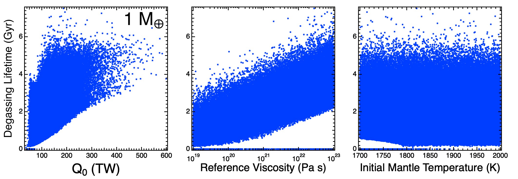
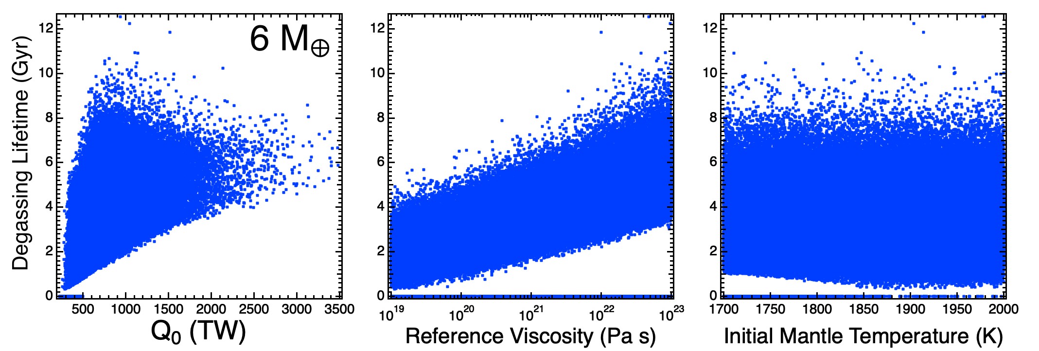
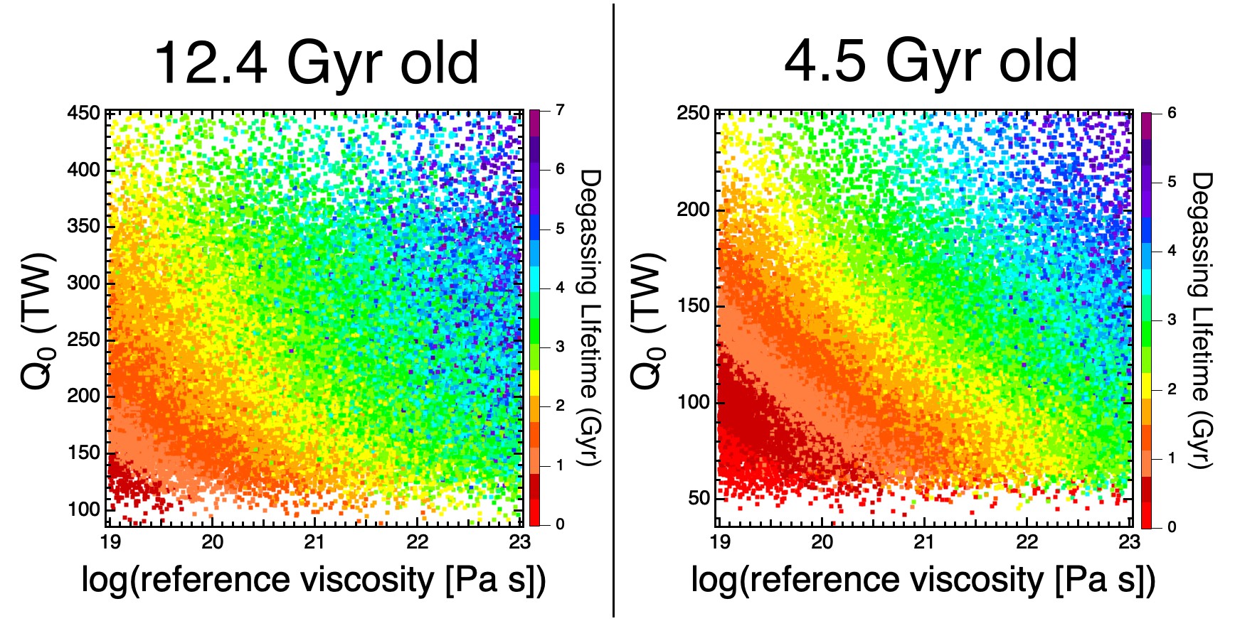
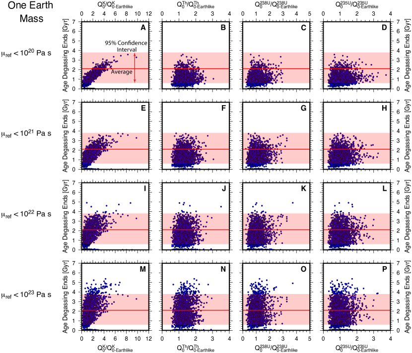
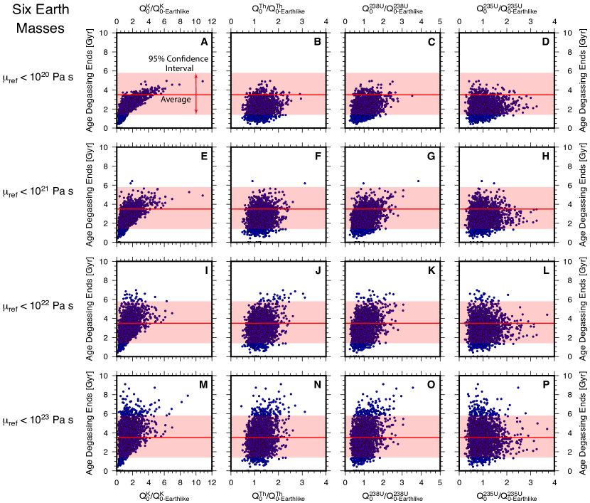
For a stagnant-lid rocky exoplanet, we find that the lifetime of mantle degassing increases with planet mass but has decreased as the Galaxy has aged (Figure 2). We find this lifetime is primarily a function of a planet’s initial radiogenic heat budget, , and the reference mantle viscosity, with little dependence on the initial mantle temperature or the planet’s central Fe-core mass fraction (Figures 5 and 6), similar to Foley & Smye (2018a). With higher , the planet has more heating power, and can thus stay warm enough to melt and degas for longer. As the Galaxy aged, the individual HPEs were produced and decayed at different rates, meaning the concentration a planet would inherit upon its formation and are both a function of when it formed in Galactic history (Appendix §B.1; Figure 4; Frank et al., 2014). We also find a higher reference viscosity slows mantle cooling, thereby allowing high temperatures, and therefore a greater degree of volcanism, thus allowing mantle degassing to be sustained for longer (Figure 5). A larger reference viscosity also makes the stagnant lid thicker, which reduces the rate of mantle melting, and hence outgassing. However, this latter effect is less important than the effect of greater retention of interior heat.
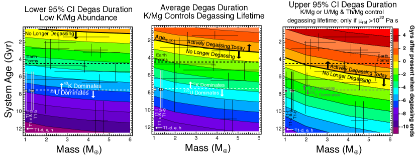
From these degassing lifetimes, we estimate the distribution of maximum current ages, Agemax, for which a stagnant-lid exoplanet will be actively degassing today ( Gyr, Figure 8). Because of the pessimistic assumptions adopted in our model, planets younger than Agemax very likely contain sufficient radiogenic heat to be degassing today, regardless of their tectonic state. Planets older than than Agemax, however, would require additional compositional or geophysical complexity to be included in our model, some of which we explore below. Adopting the average degassing lifetime for a given mass and formation time, we estimate an average maximum age, Age, for planets between 1 and 6 M⊕ to be:
| (1) |
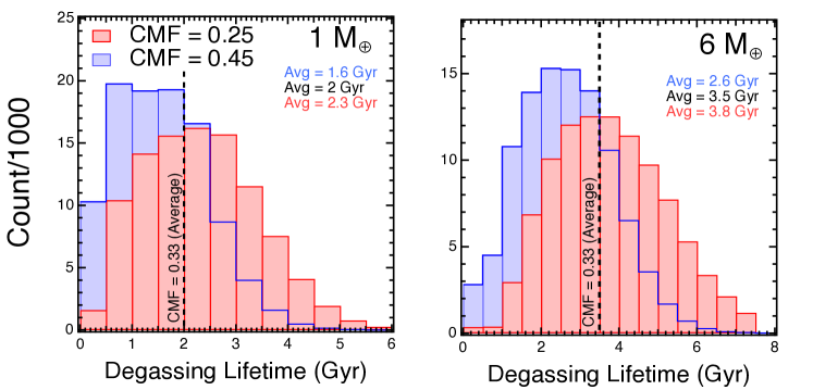
This equation incorporates the effects of Galactic chemical evolution on HPE abundance and the potential system-to-system variation in HPE concentration based on stellar abundance measurements (Figures Figure 4 and 1), reference viscosity and initial mantle temperature. From this equation, we estimate the average maximum age, Age, to be 1.8 Gyr for 1 M⊕ stagnant-lid exoplanets, increasing to 3.3 Gyr for 6 M⊕ planets (Figure 8, center).
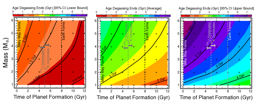
Using the upper-limit of the 95% confidence interval of our predicted degassing lifetimes for a given mass and formation time (Figure 8, right), we estimate the upper-limit of the 95% confidence interval in the maximum age, Age, for planets between 1 and 6 M⊕ to be:
| (2) |
This yields Age values of 3.7 and 6.2 Gyr for 1 and 6 M⊕ planets, respectively (Figure 8, right). These longer degassing lifetimes are primarily only relevant for planets with reference viscosities 10-100 times that of the Earth (Figure 7). Conversely, at the lower-limit of the 95% confidence interval of our predicted degassing lifetimes, 1 M⊕ planets would only be degassing today if younger than 500 Myr, with this maximum age increasing to 1 Gyr for 6 M⊕ planets (Figure 8, left).
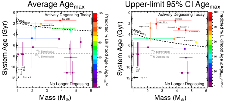
Of all exoplanets discovered to date, 694 have reported measurements of mass, radius, and host-star age, as well as the respective uncertainties in each, according to the NASA exoplanet archive (Akeson et al. (2013),https://doi.org/10.26133/NEA1 (catalog 10.26133/NEA1)). Of these, we find 17 planets (Table 2) between 1 and 6 M⊕ with average bulk densities , a density high enough to maximize the likelihood these planets are rocky without significant H2/He atmospheres (Schulze et al., 2021), and equilibrium surface temperatures below the zero-pressure melting curve of dry peridotite (1300 K, Katz et al., 2003), thus allowing a solid surface. These planets represent a range of ages between 1.4 and 11 Gyr. Assuming a planet’s mass and age form a bivariate normal distribution, we estimate the probability that these likely rocky exoplanets are younger than Agemax for their mass, and thus the likelihood they are actively degassing today. Because of the dependence of degassing lifetime on both the planet’s HPE budget and mantle reference viscosity (Figures 5, 7,9–10), and the lack of empirical constraints on mantle viscosity, we calculate Agemax using the average degassing lifetime from Figure 2 (center; Age) and the upper-bound of the 95% confidence interval (Figure 2, right; Age), which represents our least pessimistic estimate of Agemax.
We estimate only one planet, K2-36b, is younger than Age for its mass at greater than 2 (95%) confidence (Figure 3; Table 2). Additionally, at the () confidence level, Kepler 80-e is younger than Age. These planets would still require a sufficient HPE abundance to support degassing lifetimes longer than their current age, but no requirement for high mantle reference viscosity Pa s (Figures 7, 9 and 10). Adopting the more optimistic Age, three additional planets are younger than this maximum age for their mass at confidence (Kepler-80 e, Kepler-65 d and Kepler-105 c) and with confidence (Kepler-245 c and Kepler-36 b). We note though that those stagnant-lid exoplanets younger than Age would require both a sufficient HPE budget and mantle reference viscosities 10-100 times greater than the Earth’s based on our pessimistic thermal evolution models (Figures 7, 9 and 10).
The remaining 10 planets in this sample all have probabilities below 50% of being younger than Age, including the TRAPPIST-1 system. We therefore cannot confidently assume that these planets are actively degassing at a sufficient rate to sustain a temperate climate today. Our model, however, is intentionally pessimistic in its determination of Agemax. There are a number of factors, aside from the radiogenic HPE budget and planet size, that can change a planet’s degassing lifetime not included in our model. By examining the effects of these additional parameters on our model results, we can gauge the degree Agemax can change as we relax the pessimistic assumptions of our model.
3 Factors that Extend Stagnant-lid Degassing Lifetimes
Of the HPEs, 40K is the dominant element controlling the lifetime of mantle degassing (Figures 9 and 10), and thus sets Agemax for those planets likely degassing today. Unlike Th and U, a planet’s concentrations of K and 40K are not directly inferrable from abundance determinations of the host star (Appendix §B.2). 40K is a moderately volatile element, meaning its concentration relative to the rock-building elements (e.g., Mg) in a planet will be reduced compared to the host-star due to volatilization effects during planet formation. Furthermore, the host-star reveals only information on the bulk K abundance, and not the 40K/K ratio; whether the Earth’s initial 40K/K ratio of 0.1419% is universal for all rocky exoplanets is unknown. We estimate that simply doubling 40K/K would increase the distribution of Agemax by 1 Gyr (Figure 11). An effective method for altering a planet’s 40K/K is supernova injection of 40K-rich material into the protoplanetary disk prior to planet formation. Little work, however, has been done to estimate the range of possible exoplanetary 40K/K via this process. We therefore modeled the production and distribution of 40K and K in a 15 M⊙ supernovae progenitor (Appendix §B.2, Figures 12–13). We find that while the production of extremely 40K-rich material is possible, the total mass injected into the disk is unlikely to increase a protoplanet’s 40K/K by any appreciable amount, except potentially for those orbiting in low-mass, M-dwarf disks.
Mantle reference viscosity is the other key factor controlling degassing lifetime and Agemax. On average, we find degassing lifetime increases by Gyr per factor of 10 increase in reference viscosity for a 1 M⊕ planet, and by Gyr for a 6 M⊕ planet. These would then correspond to increases in Age of and Gyr per factor of 10 increase in mantle reference viscosity, respectively. Because viscosity increases with pressure (e.g., Karato & Wu, 1993; Hirth & Kohlstedt, 2003), super-Earth lower mantles can have very large viscosities (e.g., Stamenkovic et al., 2011; Tackley et al., 2013; Noack & Breuer, 2014; Schaefer & Sasselov, 2015) due to their larger core-mantle boundary pressure (Unterborn & Panero, 2019). As a result, mantle reference viscosity may, on average, increase with increasing planet size, leading to a corresponding increase in Age, such that Age may increase more sharply with planet size than our model results indicate. However, viscosity extrapolations to such extreme temperature-pressure conditions are highly uncertain (Karato, 2011). Moreover, if the increase in viscosity with depth is large enough, the lower mantles of super-Earths may cease convecting entirely.
Dorn et al. (2018) found that planets larger than 3-4 M⊕ may not experience outgassing at all, due to melt forming at a high enough pressure that it would be to dense to rise to the surface. In contrast, our models find that melt forms at low enough pressures to be buoyant regardless of planet size, unless the reference viscosity is increased to Pa s, a factor of above the upper bound in our models. Testing this very high viscosity case, we find volcanism and degassing is precluded on planets larger than M⊕, consistent with Dorn et al. (2018). A further increase in reference viscosity would prevent volcanism from ever occurring on planets of all sizes. Determining the exact cause of the difference between our results and Dorn et al. (2018) would require a detailed study with numerical convection models, and is therefore beyond this paper’s scope. However, it is likely related to the inclusion of pressure-dependent viscosity in Dorn et al. (2018); this causes higher viscosity in the lower mantle as planet size increases, potentially leading to overall less vigorous convection and thicker lithospheres that suppress melting. Mantle viscosity is therefore important in determining whether degassing is prevented on large planets due to dense melt. An additional implication of our finding on the role of mantle viscosity is that it would be difficult to extend degassing lifetimes, or Agemax, much beyond our 95% confidence interval upper limit by increasing mantle viscosity, especially for larger planets; these high viscosities would instead prevent degassing entirely.
Reference viscosity is also influenced by planet composition, including both the relative abundances of the major rock-forming elements (Mg, Si, Fe) and the oxidation state of these elements. Fayalite (Fe2SiO4) has a lower viscosity by a factor of than forsterite (Mg2SiO4 and the dominant component of Earth’s mantle), meaning a more FeO-rich mantle will have a lower viscosity than an Mg-rich one (Zhao et al., 2009), likely lowering Agemax. Mantle FeO content, however, also decreases the melting temperature of the mantle, making melting and degassing easier. More in-depth models are needed to analyze these counter-acting effects. Viscosity will also depend on silica (SiO2) content, with a lower Mg/Si leading to a higher viscosity (Ballmer et al., 2017; Spaargaren et al., 2020). However, the effect is limited, as even a very silica-rich planet with Mg/Si = 0.5 only has a factor of higher viscosity than the Earth (Spaargaren et al., 2020). Silica-rich planets may therefore have a slightly higher distribution of Agemax than those with an Earth-like planet composition considered in our model. Studies of stellar abundances, however, predict mantles with such a low mantle Mg/Si due to silica enrichment are very rare (Unterborn & Panero, 2019; Spaargaren et al., 2020).
Finally, mantle volatile content, in particular water, is known from rock deformation experiments to have a significant effect on viscosity (e.g., Hirth & Kohlstedt, 1996), with the viscosity of mantle rock decreasing with increasing water content. At the same time, water content also affects the mantle solidus, with melting temperatures decreasing as mantle water content increases (e.g., Kushiro et al., 1968). These two effects counteract each other. The same is true for other compositional factors, such as mantle Fe content (Dorn et al., 2018). Ultimately, to fully capture these competing effects, new models incorporating the combined compositional effects on viscosity and solidus would be needed. However, we provide a first-order estimate of how Agemax changes with mantle water content, based on model suites where mantle solidus and reference viscosity are systematically varied using the solidus parameterization of Katz et al. (2003) and the diffusion creep viscosity flow laws of Hirth & Kohlstedt (2003) (Appendix B.4).
For water contents wt%, the effect of water lowering mantle viscosities dominates, causing Age to decrease compared to a dry-planet baseline as the lower viscosity leads to more rapid cooling (Figure 15). Above these water contents, the decrease in solidus temperature begins to dominate, and Age begins to increase in comparison to a dry planet baseline as mantle melting can occur at lower temperatures. For a 1 M⊕ planet, we find Age can be lowered by at most Gyr for moderate water contents ( wt%), and raised by up to Gyr for higher water contents ( wt%), with the exact change depending on the chosen water-viscosity dependency exponent, (Figure 15). These effects are more pronounced for a 6 M⊕ planet. These estimates are likely upper limits, as we do not include overburden pressure of surface water, which will lower the rate of, or entirely prevent, volcanism (Kite et al., 2009; Cowan & Abbot, 2014; Krissansen-Totton et al., 2021), as well as the evolution of in- and outgassing rates of water over time (e.g., McGovern & Schubert, 1989; Crowley et al., 2011; Spaargaren et al., 2020).
The addition of tidal heating (e.g., Barnes et al., 2009; Driscoll & Barnes, 2015) or magnetic induction heating (e.g., Kislyakova et al., 2017) would also prolong mantle degassing and increase Agemax beyond our model estimates. Both of these sources of heat depend on a planet’s orbit, and will persist as long as the orbital configuration allows, unlike radiogenic heat sources which decay over time. Planets heated by tides or magnetic induction can therefore sustain degassing for very long times, potentially even indefinitely. Exoplanetary orbit parameters can be constrained observationally, so the likelihood of significant tidal or magnetic induction heating can be estimated in most cases.
As explained above, our model makes pessimistic assumptions that err on the side of hastening the end of volcanism, including neglecting mantle plumes and assuming all melt erupts at the surface. We found that varying melt intrusion did not significantly change our results; 90% melt intrusion increases our estimated degassing lifetime by only Myrs for an Earth mass planet. Mantle plumes, however, can prolong volcanism, even after the upper mantle has cooled below the point where it can melt through passive upwelling, depending on the temperature difference between plume and surrounding mantle. While the effect of plumes can only be fully captured with higher dimensional dynamic models, we can roughly approximate how much they might extend degassing lifetime based on our models where mantle solidus temperature was varied (Figure 14). There we found a 100∘C decrease in solidus temperature increases degassing lifetime by Gyrs for a 1 M⊕ planet. Therefore if upwelling plumes are 100-300∘C hotter than surrounding mantle, as estimated for Earth (White & McKenzie, 1995; Shen et al., 1998; Thompson & Gibson, 2000), degassing could last up to Gyr longer. If plume volcanism is as active as Earth, then it likely could maintain sufficient CO2 outgassing for maintaining a temperate climate, as plume volcanism accounts for of the CO2 degassing on Earth (Marty & Tolstikhin, 1998). Plume activity may be more muted on stagnant lid planets, however, as inefficient mantle cooling leads to a smaller temperature anomaly for plumes (O’Rourke & Korenaga, 2015), so the estimates given here for how plumes prolong volcanism should be considered upper bounds.
Our model predictions can also be applied to Venus, assuming it is a stagnant-lid planet. Venus is a 0.82 M⊕ planet, meaning our model predicts average and upper-limit Agemax values of 1.6 and 3.5 Gyr, respectively. That is, it should not exhibit significant enough volcanism and outgassing today to support a temperate climate ( 10% Earth’s present rate). There is some evidence, however, for volcanism and outgassing in the last 1 Myr (Smrekar et al., 2010; Filiberto et al., 2020; Byrne & Krishnamoorthy, 2022), likely plume related (Gülcher et al., 2020). If corroborated, this would not necessarily invalidate the model predictions, as rates of Venusian volcanism are probably too low to support outgassing rates above our threshold rate of degassing to support a temperate climate. Estimates of the rate of volcanism on Venus, if present, are uncertain, but most fall in the range of 0.1–1 km3 yr-1 with a highest estimate of 10 km3 yr-1 (Fegley & Prinn, 1989; Byrne & Krishnamoorthy, 2022, and references therin). These volcanism rates are therefore 30–300 times lower (with a minimum of 2 times lower for the highest rate for Venus) than Earth’s estimated 26-34 km3 yr-1 (Crisp, 1984), and would lead to comparably lower CO2 outgassing rates. Only the upper end estimate of km3 yr-1 would be large enough to drive CO2 outgassing at a rate 10% the modern Earth’s. Moreover, it is possible that Venus is experiencing volcanism due to lying in a tectonic regime intermediate to stagnant lid and plate tectonic end members, and therefore having a thinner lithosphere than expected for a purely stagnant-lid planet. There is evidence for limited plate-tectonics-like subduction (Sandwell & Schubert, 1992; Davaille et al., 2017) and relative movement of crustal blocks on the surface (Byrne et al., 2021), as well a relatively thin lithosphere and high heat flux, compared to pure stagnant-lid models (Borrelli et al., 2021). Venus, therefore, demonstrates that planets may operate in a regime intermediate to the end-member plate tectonics and stagnant-lid regimes, leading to longer-lived volcanism than our pessimistic stagnant-lid models predict.
Plate tectonics can drastically increase the lifetime of degassing on a rocky exoplanet to ages beyond Agemax due to lithospheric thinning allowing for mantle material to melt at lower temperatures (e.g. Kite et al., 2009). For planets significantly older than where tidal or induction heating are unlikely, our stagnant-lid framework would not be able to explain any atmospheric observations showing atmospheric chemistries indicative of active mantle degassing or the presence of a temperate climate. These older planets, then, may provide an ideal sample to search for rocky exoplanets undergoing plate tectonics similar to Earth, or indicate planets with complex tectonic histories that have potentially transitioned between different tectonic modes over time.
Our definition of Agemax represents a pessimistic upper-limit of the “temporal habitable zone” for rocky, stagnant-lid exoplanets not undergoing tidal heating. For planets older than this “zone”, we estimate they will have exhausted their internal radiogenic heat budget to the point where interior melting is limited and mantle degassing rates are no longer sufficient to support a temperate climate today, when we observe it. Other compositional and dynamical factors may increase Agemax for these stagnant-lid planets, as described above, however, they are often fraught with other complications that may impact other aspects of planetary habitability.
4 Conclusion
An individual rocky exoplanet provides us with a sparseness of direct data with which to understand its evolution. Host-star age and radionuclide abundance, while indirectly telling us about the planet, are critical, and currently underutilized, observables that will allow us to better understand both an exoplanet’s history and its current likelihood of being temperate today, regardless of tectonic state. The framework we present here that combines direct and indirect observational data with dynamical models not only provide us with a pessimistic baseline for understanding which parameter(s) most control a stagnant-lid exoplanet’s ability to support a temperate climate, but also where more lab-based and computational work is needed to quantify the reasonable range of these parameters (e.g., mantle reference viscosity). As we move to more in-depth characterization of individual targets in the James Webb Space Telescope era, these direct and indirect astronomic observables coupled with laboratory data and models from the geoscience community will allow us to better estimate whether a rocky exoplanet planet in both the canonical and temporal habitable zones, or has exhausted its internal heat and is simply too old to be “Earth-like.”
Acknowledgements
CTU acknowledges the support of Arizona State University through the SESE Exploration fellowship. The results reported herein benefited from collaborations and/ or information exchange within NASA’s Nexus for Exoplanet System Science (NExSS) research coordination network sponsored by NASA’s Science Mission Directorate, and gratefully acknowledge support from grant NNX15AD53G awarded to SD. We thank the anonymous reviewer for their helpful comments which improved the manuscript’s clarity considerably.
References
- Abbot et al. (2012) Abbot, D. S., Cowan, N. B., & Ciesla, F. J. 2012, Astrophys. J., 756, 178, doi: 10.1088/0004-637X/756/2/178
- Akeson et al. (2013) Akeson, R. L., Chen, X., Ciardi, D., et al. 2013, PASP, 125, 989, doi: 10.1086/672273
- Ballmer et al. (2017) Ballmer, M. D., Houser, C., Hernlund, J. W., Wentzcovitch, R. M., & Hirose, K. 2017, Nature Geoscience, 10, 236, doi: 10.1038/ngeo2898
- Barnes et al. (2009) Barnes, R., Jackson, B., Raymond, S., West, A., & Greenberg, R. 2009, The Astrophysical Journal, 695, 1006
- Bercovici et al. (2015) Bercovici, D., Tackley, P., & Ricard, Y. 2015, in Treatise on Geophysics, ed. D. Bercovici & G. Schubert (chief editor), Vol. 7, Mantle Dynamics (New York: Elsevier), 271–318
- Borrelli et al. (2021) Borrelli, M. E., O’Rourke, J. G., Smrekar, S. E., & Ostberg, C. M. 2021, Journal of Geophysical Research (Planets), 126, e06756, doi: 10.1029/2020JE006756
- Botelho et al. (2019) Botelho, R. B., Milone, A. d. C., Meléndez, J., et al. 2019, MNRAS, 482, 1690, doi: 10.1093/mnras/sty2791
- Breuer & Moore (2015) Breuer, D., & Moore, W. 2015, in Treatise on Geophysics (Second Edition), second edition edn., ed. G. Schubert (Oxford: Elsevier), 255 – 305, doi: https://doi.org/10.1016/B978-0-444-53802-4.00173-1
- Byrne et al. (2021) Byrne, P. K., Ghail, R. C., Celâl Şengör, A. M., et al. 2021, Proceedings of the National Academy of Science, 118, 2025919118, doi: 10.1073/pnas.2025919118
- Byrne & Krishnamoorthy (2022) Byrne, P. K., & Krishnamoorthy, S. 2022, Journal of Geophysical Research: Planets, 127, e2021JE007040, doi: 10.1029/2021JE007040
- Cowan & Abbot (2014) Cowan, N. B., & Abbot, D. S. 2014, Astrophys. J., 781, 27, doi: 10.1088/0004-637X/781/1/27
- Crisp (1984) Crisp, J. A. 1984, J. Volcanol. Geotherm. Res., 20, 177, doi: 10.1016/0377-0273(84)90039-8
- Crowley et al. (2011) Crowley, J. W., Gérault, M., & O’Connell, R. J. 2011, EPSL, 310, 380, doi: 10.1016/j.epsl.2011.08.035
- Davaille et al. (2017) Davaille, A., Smrekar, S. E., & Tomlinson, S. 2017, Nature Geoscience, 10, 349, doi: 10.1038/ngeo2928
- Dorn et al. (2018) Dorn, C., Noack, L., & Rozel, A. B. 2018, Astron. Astrophys., 614, A18, doi: 10.1051/0004-6361/201731513
- Driscoll & Barnes (2015) Driscoll, P. E., & Barnes, R. 2015, Astrobiology, 15, 739
- Fegley & Prinn (1989) Fegley, B., & Prinn, R. G. 1989, Nature, 337, 55, doi: 10.1038/337055a0
- Filiberto et al. (2020) Filiberto, J., Trang, D., Treiman, A. H., & Gilmore, M. S. 2020, Science Advances, 6, eaax7445, doi: 10.1126/sciadv.aax7445
- Foley (2019) Foley, B. J. 2019, Astrophys. J., 875, 72, doi: 10.3847/1538-4357/ab0f31
- Foley et al. (2012) Foley, B. J., Bercovici, D., & Landuyt, W. 2012, Earth Planet. Sci. Lett., 331–332, 281 , doi: 10.1016/j.epsl.2012.03.028
- Foley & Driscoll (2016) Foley, B. J., & Driscoll, P. E. 2016, Geochem., Geophys., Geosyst., 17, doi: 10.1002/2015GC006210
- Foley & Smye (2018) Foley, B. J., & Smye, A. J. 2018, Astrobiology, 18, 873, doi: 10.1089/ast.2017.1695
- Frank et al. (2014) Frank, E. A., Meyer, B. S., & Mojzsis, S. J. 2014, Icarus, 243, 274, doi: 10.1016/j.icarus.2014.08.031
- Gülcher et al. (2020) Gülcher, A. J. P., Gerya, T. V., Montési, L. G. J., & Munch, J. 2020, Nature Geoscience, 13, 547, doi: 10.1038/s41561-020-0606-1
- Haqq-Misra et al. (2016) Haqq-Misra, J., Kopparapu, R. K., Batalha, N. E., Harman, C. E., & Kasting, J. F. 2016, Astrophys. J., 827, 120, doi: 10.3847/0004-637X/827/2/120
- Hinkel et al. (2014) Hinkel, N. R., Timmes, F., Young, P. A., Pagano, M. D., & Turnbull, M. C. 2014, AJ, 148, 54. http://stacks.iop.org/1538-3881/148/i=3/a=54
- Hirth & Kohlstedt (1996) Hirth, G., & Kohlstedt, D. 1996, Earth Planet. Sci. Lett., 144, 93
- Hirth & Kohlstedt (2003) —. 2003, in Subduction Factory Mongraph, ed. J. Eiler, Vol. 138 (Washington, DC: Am. Geophys. Union), 83–105
- Kadoya & Tajika (2014) Kadoya, S., & Tajika, E. 2014, Astrophys. J., 790, 107, doi: 10.1088/0004-637X/790/2/107
- Karato (2011) Karato, S. 2011, Icarus, 212, 14 , doi: 10.1016/j.icarus.2010.12.005
- Karato & Wu (1993) Karato, S., & Wu, P. 1993, Science, 260, 771, doi: 10.1126/science.260.5109.771
- Kasting & Catling (2003) Kasting, J. F., & Catling, D. 2003, Annu. Rev. Astron. Astrophys., 41, 429, doi: 10.1146/annurev.astro.41.071601.170049
- Kasting et al. (1993) Kasting, J. F., Whitmire, D. P., & Reynolds, R. T. 1993, Icarus, 101, 108, doi: 10.1006/icar.1993.1010
- Katz et al. (2003) Katz, R. F., Spiegelman, M., & Langmuir, C. H. 2003, Geochem., Geophys., Geosyst., 4, 1073, doi: 10.1029/2002GC000433
- Kislyakova et al. (2017) Kislyakova, K. G., Noack, L., Johnstone, C. P., et al. 2017, Nature Astronomy, 1, 878, doi: 10.1038/s41550-017-0284-0
- Kite & Ford (2018) Kite, E. S., & Ford, E. B. 2018, ApJ, 864, 75, doi: 10.3847/1538-4357/aad6e0
- Kite et al. (2009) Kite, E. S., Manga, M., & Gaidos, E. 2009, ApJ, 700, 1732, doi: 10.1088/0004-637X/700/2/1732
- Kopparapu et al. (2013) Kopparapu, R. K., Ramirez, R., Kasting, J. F., et al. 2013, The Astrophysical Journal, 765, 131
- Krissansen-Totton et al. (2021) Krissansen-Totton, J., Galloway, M. L., Wogan, N., Dhaliwal, J. K., & Fortney, J. J. 2021, ApJ, 913, 107, doi: 10.3847/1538-4357/abf560
- Kushiro et al. (1968) Kushiro, I., Syono, Y., & Akimoto, S. 1968, J. Geophys. Res., 73, 6023
- Marty & Tolstikhin (1998) Marty, B., & Tolstikhin, I. N. 1998, Chem. Geol., 145, 233
- McGovern & Schubert (1989) McGovern, P., & Schubert, G. 1989, Earth and planetary science letters, 96, 27
- Menou (2015) Menou, K. 2015, Earth Planet. Sci. Lett., 429, 20, doi: 10.1016/j.epsl.2015.07.046
- Nimmo et al. (2020) Nimmo, F., Primack, J., Faber, S. M., Ramirez-Ruiz, E., & Safarzadeh, M. 2020, ApJL, 903, L37, doi: 10.3847/2041-8213/abc251
- Noack & Breuer (2014) Noack, L., & Breuer, D. 2014, Planetary and Space Science, 98, 41
- O’Neill & Lenardic (2007) O’Neill, C., & Lenardic, A. 2007, Geophys. Res. Lett., 34, 19204, doi: 10.1029/2007GL030598
- Oosterloo et al. (2021) Oosterloo, M., Höning, D., Kamp, I. E. E., & van der Tak, F. F. S. 2021, arXiv e-prints, arXiv:2103.09505. https://arxiv.org/abs/2103.09505
- O’Rourke & Korenaga (2015) O’Rourke, J. G., & Korenaga, J. 2015, Icarus, 260, 128, doi: 10.1016/j.icarus.2015.07.009
- Sandwell & Schubert (1992) Sandwell, D. T., & Schubert, G. 1992, Science, 257, 766, doi: 10.1126/science.257.5071.766
- Schaefer & Sasselov (2015) Schaefer, L., & Sasselov, D. 2015, Astrophys. J., 801, 40, doi: 10.1088/0004-637X/801/1/40
- Schulze et al. (2021) Schulze, J. G., Wang, J., Johnson, J. A., et al. 2021, Plan. Sci. Journal, 2, 113, doi: 10.3847/PSJ/abcaa8
- Shen et al. (1998) Shen, Y., Solomon, S. C., Bjarnason, I. T., & Wolfe, C. J. 1998, Nature, 395, 62, doi: 10.1038/25714
- Sleep & Zahnle (2001) Sleep, N. H., & Zahnle, K. 2001, J. Geophys. Res., 106, 1373, doi: 10.1029/2000JE001247
- Smrekar et al. (2010) Smrekar, S. E., Stofan, E. R., Mueller, N., et al. 2010, Science, 328, 605, doi: 10.1126/science.1186785
- Spaargaren et al. (2020) Spaargaren, R. J., Ballmer, M. D., Bower, D. J., Dorn, C., & Tackley, P. J. 2020, A&A, 643, A44, doi: 10.1051/0004-6361/202037632
- Stamenkovic et al. (2011) Stamenkovic, V., Breuer, D., & Spohn, T. 2011, Icarus, 216, 572 , doi: 10.1016/j.icarus.2011.09.030
- Tackley et al. (2013) Tackley, P. J., Ammann, M., Brodholt, J. P., Dobson, D. P., & Valencia, D. 2013, Icarus, 225, 50, doi: 10.1016/j.icarus.2013.03.013
- Thompson & Gibson (2000) Thompson, R. N., & Gibson, S. A. 2000, Nature, 407, 502, doi: 10.1038/35035058
- Unterborn et al. (2015) Unterborn, C. T., Johnson, J. A., & Panero, W. R. 2015, ApJ, 806, 139, doi: 10.1088/0004-637X/806/1/139
- Unterborn & Panero (2019) Unterborn, C. T., & Panero, W. R. 2019, Journal of Geophysical Research (Planets), 124, 1704, doi: 10.1029/2018JE005844
- Valencia et al. (2007) Valencia, D., O’Connell, R. J., & Sasselov, D. D. 2007, Astrophys. J., 670, L45, doi: 10.1086/524012
- van Heck & Tackley (2011) van Heck, H. J., & Tackley, P. J. 2011, Earth Planet. Sci. Lett., 310, 252, doi: 10.1016/j.epsl.2011.07.029
- Walker et al. (1981) Walker, J., Hayes, P., & Kasting, J. 1981, J. Geophys. Res., 86, 9776, doi: 10.1029/JC086iC10p09776
- White & McKenzie (1995) White, R. S., & McKenzie, D. 1995, J. Geophys. Res., 100, 17,543, doi: 10.1029/95JB01585
- Zhao et al. (2009) Zhao, Y.-H., Zimmerman, M. E., & Kohlstedt, D. L. 2009, Earth Planet. Sci. Lett., 287, 229, doi: 10.1016/j.epsl.2009.08.006
Appendix A Methods
We adopt the stagnant-lid thermal evolution model of Foley & Smye (2018a); Foley (2019) updated to account for a planet’s mass, core mass fraction (CMF), metamorphic degassing rate, individual HPE contents, fractionation of HPEs into the crust and solidus changes due to mantle depletion (Appendices §A.1 and §A.2). In these models, initial radioactive heat production budgets are determined in a Monte-Carlo fashion sampling within the observed variability of HPEs in FGK stars, corrected for fractionation and volatility effects (Appendix §A.3). We define the cessation of degassing as the moment when a planet’s degassing rate first falls below 10% of the Earth’s present day degassing rate ( mol yr-1, Marty & Tolstikhin, 1998), scaled linearly by planet surface area. Foley (2019) confirmed that degassing rates must be % the modern day Earth’s for a temperate climate on stagnant-lid planets, even if the planet is mostly ocean covered and thus dominated by seafloor weathering. Seafloor weathering has an overall slower rate than continental weathering on the modern Earth, and thus with only seafloor weathering active atmospheric CO2 levels (and surface temperatures) would be higher, for a given degassing rate (e.g., Krissansen-Totton & Catling, 2017; Hayworth & Foley, 2020; Glaser et al., 2020). Planets with higher land fractions would thus require higher degassing rates than our chosen threshold to remain temperate. Moreover, our degassing rate threshold was determined for a planet receiving a stellar radiative flux equal to what Earth receives today. Lower incoming radiative fluxes would also require higher rates of degassing than our assumed threshold in order to sustain temperate climates.
We scale our degassing rate threshold with planet surface area, because the total weathering rate increases linearly with the area of weatherable rock. Thus a planet with a larger surface area will need a proportionally higher degassing rate to sustain a temperate climate. Ultimately, planets with degassing rates below our threshold for temperate climates may not be the best targets for atmospheric characterization or detectable surface life, as they are likely to lie in snowball climate states. Finally, another climate extreme is possible if the rate of CO2 degassing overwhelms the surface weathering rate; this will produce a hot-house, Venus-like climate.
A.1 Updates to Thermal Evolution Model
Foley & Smye (2018a) and Foley (2019) give a thorough description of our model, and all of the key governing equations are listed in Appendix §A.2. Here we will only highlight the differences between the model of Foley & Smye (2018a) and the model presented in this paper. For an Earth-like CMF = 0.33, we use the scaling laws from Valencia et al. (2006) & Valencia et al. (2007) to determine average mantle density, planet radius, mantle thickness, and surface gravity as a function of planet mass:
| (A1) |
| (A2) |
| (A3) |
| (A4) |
where is the planet mass and is the gravitational constant. Reference Earth values are kg m-3, km, and km.
To vary the core mass fraction, we use the scaling laws from Noack et al. (2016) (See also: Foley et al. (2020)), which assume that all iron resides in the core. The resulting equations for , , and , as a function of CMF and planet mass, are:
| (A5) |
| (A6) |
| (A7) |
Gravity is still calculated from A4.
We assume all other material properties are independent of planet size and CMF. This is a simplification because thermal conductivity, expansivity, and viscosity are all functions of pressure, and the larger the planet or larger the core, the higher the pressures reached in the mantle. However, robust parameterizations for how to incorporate these pressure effects are currently lacking. There is still significant uncertainty about how key material properties change at the extreme temperature and pressure conditions of super-Earth lower mantles, which are not yet experimentally accessible (e.g., Duffy et al., 2015). Moreover, how significant variation of key material properties with pressure, and hence depth in a super-Earth mantle, modifies the dynamics of the convecting mantle has not been extensively studied; scaling laws for convective heat flux and velocity that take these pressure effects into account have not yet been developed.
Lacking robust parameterizations for viscosity, thermal expansivity, and thermal conductivity pressure effects, we instead randomly vary the mantle reference viscosity, , in our models over a four-orders-of-magnitude range. We focus on viscosity because, of the key mantle material properties, it shows the strongest dependence on pressure and mantle composition, as it can vary by orders of magnitude (e.g., Karato & Wu, 1993; Hirth & Kohlstedt, 2003). We use a standard Arrhenius temperature-dependent viscosity law in our models:
| (A8) |
where is mantle interior viscosity, is mantle potential temperature, kJ mol-1 (e.g., Karato & Wu, 1993) is activation energy, and is the universal gas constant. The reference viscosity is defined at reference temperature K, or approximately Earth’s present day mantle potential temperature. The constant is then adjusted in each model run to match the chosen reference viscosity. Our results therefore explicitly demonstrate how degassing lifetime depends on mantle reference viscosity, which itself may vary with planet size or composition.
The equations for calculating the rate of metamorphic degassing due to crustal burial, from Foley & Smye (2018a), are reformulated in terms of pressure, rather than depth (see Appendix §A.2.3). As such they can then be applied to planets with variable size and CMF, and hence different surface gravities. Finally, we have improved the melting model to include depletion of the mantle and a subsequent increase in the melting temperature. We follow the method of Tosi et al. (2017), and assume the solidus can increase by up to 150 K upon full depletion of the mantle, the difference in the solidi of harzburgite and peridotite. The degree of mantle depletion is calculated based on the volume of crust present at each timestep (see Appendix §A.2.1). The model also tracks each of the four major HPEs separately, rather than treating them together with an average decay constant as in Foley & Smye (2018a). Here we are interested in observationally constrained variations in each of the four major HPEs, so we naturally must treat each HPE separately in the model (see Appendix §A.2.1). The remainder of the model equations are general and can be applied to planets with different masses and core mass fractions.
A.2 Thermal Evolution Model
Here we give a complete description of the coupled thermal evolution and volatile cycling model. Assuming pure internal heating, and that all melt produced contributes to cooling of the mantle, mantle thermal evolution is given by:
| (A9) |
where is the volume of the actively convecting mantle, the average density of the mantle, the heat capacity, the potential temperature of the mantle, time, the total radiogenic heat production rate of the mantle, the surface area of the top of the convecting mantle (base of the stagnant-lid), the heat flux from the mantle, the volumetric melt production rate, the density of melt, the temperature difference between erupted melt and the surface temperature, and the latent heat of the mantle (e.g., Stevenson et al., 1983; Hauck & Phillips, 2002; Reese et al., 2007; Fraeman & Korenaga, 2010; Morschhauser et al., 2011; Driscoll & Bercovici, 2014; Foley & Smye, 2018a; Foley, 2019). The volume of the convecting mantle is , where is the planet radius, is the core radius, and the thickness of the stagnant-lid. The surface area of the top of the convecting mantle is then . Finally, the temperature difference between erupted melt and the surface temperature is , where is the average adiabatic temperature gradient of mantle melt, estimated as K Pa-1 in Foley & Smye (2018a), and is the pressure where melting begins (derived below in §A.2.1).
The thickness of the stagnant-lid, , is then (e.g., Schubert et al., 1979; Spohn, 1991):
| (A10) |
where is the temperature at the base of the stagnant-lid, is the thermal conductivity (assumed to be the same throughout the crust and mantle for simplicity), and is the height above the planet’s center. The mantle heat flux, , and lid base temperature, , are calculated from the following scaling laws for stagnant-lid convection (Reese et al., 1998, 1999; Solomatov & Moresi, 2000; Korenaga, 2009):
| (A11) |
and
| (A12) |
where and are constants (assumed to be and ), and is the surface temperature, here fixed to 273 K, as surface temperature fluctuations of order 100 K, that could result from changes in atmospheric CO2, do not significantly impact the evolution of the underlying mantle in these models (Foley, 2019). The mantle thickness is , and is the Frank-Kamenetskii parameter, , where is the activation energy for mantle viscosity and is the universal gas constant. The internal Rayleigh number, , is defined as , where is gravity, the thermal expansivity of the mantle, the thermal diffusivity of the mantle, and the viscosity at the mantle potential temperature of (see Equation A8).
A.2.1 Melting and Crustal Evolution
Large-scale mantle melting, and subsequent volcanism, takes place when passively upwelling mantle is hot enough to cross the solidus beneath the lid. As in (e.g., Fraeman & Korenaga, 2010; Foley & Smye, 2018a), the pressure at which melting begins, , is calculated from the intersection of the mantle adiabat, with adiabatic gradient , and the dry peridotite solidus from Takahashi & Kushiro (1983):
| (A13) |
where is the melting solidus temperature at 0 pressure, and the adiabatic gradient in the mantle is K Pa-1. The solidus temperature at 0 pressure depends on the degree of mantle depletion, which we estimate based on the volume of crust present, as explained below. We also do not allow the pressure where melting begins to exceed 10 GPa, the approximate pressure where silicate melts become denser than solids (e.g. Dorn et al., 2018). Melting stops at the base of the lid, which occurs at pressure
| (A14) |
where is the average density of the crust and lithosphere (assumed to be kg m-3). The melt fraction, , is
| (A15) |
where Pa-1. The melt production rate, , is calculated as (see Foley & Smye (2018a) for a derivation)
| (A16) |
where is the characteristic convecting mantle velocity and is the depth where melting begins. The convecting mantle velocity is (Reese et al., 1998, 1999; Solomatov & Moresi, 2000; Korenaga, 2009):
| (A17) |
where is a constant.
Melting produces a crust whose thickness, , and volume, , evolve over time. To calculate the evolution of the we assume that all melt produced contributes to growth of the crust, and that all crust buried to depths below the lithospheric thickness, , founders into the mantle. The resulting equation is
| (A18) |
The second term on the right-hand side of A18 describes the rate of crust loss due to foundering of the crust; the hyperbolic tangent function formulation allows this crust loss rate to go to 0 when . The term captures the loss of crust when the lid thickness is decreasing and , and is 0 otherwise (that is, if either the lid thickness is growing or the crust ends before the base of the stagnant-lid). The crustal thickness is calculated from the volume of crust as
| (A19) |
To incorporate how depletion of the mantle influences the solidus, and thus later melt production, we increase linearly with crust thickness following (Tosi et al., 2017):
| (A20) |
Here 1423 K is the dry peridotite solidus temperature at 0 pressure from Takahashi & Kushiro (1983). K is the increase in the solidus upon full depletion (which is set here to the difference in the zero pressure solidus temperatures for peridotite and harzburgite), and is the reference crust thickness produced upon full depletion of the mantle. Here and is the surface area of the planet. The solidus can thus increase by up to 150 K due to mantle depletion. We explore other compositional effects that affect the solidus (e.g., water) in the main text.
HPEs are preferentially partitioned into the crust during mantle melting, due to their incompatible nature. We track this partitioning for all 4 long-lived HPEs assuming accumulated fractional melting. The evolution of crustal heat production rate, for a given HPE, is thus:
| (A21) |
Here, is the heat production rate in the crust resulting from one of the four HPEs tracked in the model. The total crustal heat production rate, . Each heat producing element (HPE) has a specified decay constant, , distribution coefficient, , and crustal and mantle heat production rate per unit volume, and , respectively (e.g., is the decay constant for 238U, the distribution coefficient for 238U, and the heat production per unit volume in the crust due to 238U). The well known half-lives taken from Turcotte & Schubert (2002), are used to calculate the decay constants, . The chosen distribution coefficients of and are from Beattie (1993), and is from Hart & Brooks (1974) assuming % olivine and 40 % pyroxene in the mantle. The evolution of mantle heat production from a given radioactive isotope is:
| (A22) |
As before, the total heat production rate of the mantle, . The total heat production rates per unit volume in the crust and mantle are also sums of the heat production rates of the four HPEs: and .
A.2.2 Crustal Geotherm
Equation A10 requires as an input the conductive heat flux at the base of the lid. The temperature profile for steady-state one-dimensional heat conduction with constant heat production rates in the crust and mantle, neglecting advection, is used to determine this heat flux (for details see: Foley & Smye, 2018a):
| (A23) |
when , and
| (A24) |
when . The temperature at the base of the crust, , is
| (A25) |
The mantle radiogenic heating rate, per unit volume, , where is the volume of the sub-crustal stagnant-lid. The crustal radiogenic heat rate per unit volume is , where is the total radiogenic heating rate in the crust, and is the volume of the crust.
A.2.3 CO2 Outgassing Rates
CO2 is outgassed to the atmosphere due to both mantle melting, and subsequent volcanism, and metamorphic breakdown of carbonated minerals as the crust is buried (Foley & Smye, 2018a; Foley, 2019). Foley & Smye (2018a) showed that the temperature, as a function of depth, where metamorphic decarbonation occurs can be approximated as a simple linear relationship,
| (A26) |
where K Pa-1, K, is temperature in Kelvin, and kg m-3 is the lithosphere density. The depth where decarbonation occurs, , is (for details see: Foley & Smye, 2018a)
| (A27) |
With the decarbonation depth determined by A27, the metamorphic outgassing flux is given by
| (A28) |
where is the size of the crustal CO2 reservoir (in moles), and the hyperbolic tangent function allows to go to zero when , and to when . The outgassing rate due to mantle melting is
| (A29) |
where is the size of the mantle CO2 reservoir, and is the distribution coefficient for CO2 (Hauri et al., 2006). The evolution of the mantle and crustal reservoirs, when crustal decarbonation is active (e.g., ), follow
| (A30) |
| (A31) |
while when crustal decarbonation is inactive ()
| (A32) |
| (A33) |
The total CO2 budget of the mantle and crust, , is conserved, such that . As in Foley & Smye (2018a), the planet starts with all of the CO2 residing in the mantle, and CO2 is outgassed over time to the surface. The entire allotment of each HPE also initially resides in the mantle, as before planetary evolution begins we assume that there is no crust present (crust formation does not take place until mantle convection, and subsequent volcanism, begins). The abundance of each HPE is linked to the stellar observed abundances, as explained in Appendix §A.3.
Finally, an important limit for the carbon cycle and habitability is the global weathering supply limit. This limit is the upper bound on weathering rate, and is set by the rate at which CO2 drawdown would occur if all available fresh surface rock is completely carbonated as soon as it is brought to the surface. On a stagnant-lid planet, this limit is assumed to be set by volcanism. Using the average composition of basalt on Earth, the total amount of CO2 that can be drawn down by crustal carbonation is mol kg-1 of basalt (Foley, 2019). We assume the crust will have a basaltic composition, as it is a result of primary mantle melting of a peridotitic mantle. Exoplanets, however, could have different mantle bulk compositions, that would lead to different crustal compositions upon melting. However, the weathering demand, , only increases by about a factor of two for the extreme ultramafic composition end-member, peridotite, and only decreases by about a factor of two if the crust is felsic, like Earth’s continental crust. Average compositions from Taylor & McLennan (1985), for continental crust, and Warren (2016), for peridotite, were used in making these estimates. The total variation in weathering demand is thus approximately a factor of 4, from ultramafic to felsic end-members. This would not significantly change the planetary conditions (e.g., mantle CO2 budget, size, internal heat production rate, etc.) that control when planets enter a supply-limited weathering regime and thus develop hothouse climates (Foley & Smye, 2018a; Foley, 2019).
The weathering supply limit, , assuming all erupted basalt is available for weathering, is
| (A34) |
with units of mol yr-1; is the fraction of mantle melt produced that erupts at the surface ( is assumed). In the models, supply-limited weathering is assumed to lead to an inhospitable, hothouse climate when mol yr-1 at any point during planetary evolution, as in Foley & Smye (2018a). The total outgassing rate exceeding the weathering supply limit by mol yr-1 means that hot climates, with K, would form in Myr, well within the typical degassing lifetimes of modeled planets.
A.3 Input Radionuclide Abundances
We define the initial total heat production rate of the mantle, , as a function of the specific power () produced by each HPE (), their concentration within the planet () and the mass of the mantle (). We calculate the initial HPE abundance as . In order to quantify the range of HPE concentrations in rocky exoplanets (), we randomly sample within the observationally-constrained stellar abundance distributions for each HPE (Figure 1 of main text) and apply the scaling relationship to convert from stellar abundance to mantle concentration as a function of planet formation time, , after the birth of the Milky Way:
| (A35) |
where , are the concentrations of the element in the randomly selected stellar abundance and the Sun, respectively, and is a correction for volatility effects during planet formation. represents the predicted initial concentration of an HPE if it was a “coscmochemically Earth-like” planet (Frank et al., 2014) forming at some (Figure 4). We re-scale the results of Frank et al. (2014) such that the Earth-like abundance of each HPE at the time the Earth formed ( Gyr) are that of Palme & O’Neill (2003). This lowers our choice of by % for each HPE compared to those presented in Frank et al. (2014), who adopted the initial Earth HPE abundances of Turcotte & Schubert (2002).
We define the concentration of an HPE in both stars and the Sun as its molar ratio with Mg (e.g., X/Mg). We normalize relative to Mg as it is more likely to remain in the mantle, as opposed to Si which may partition into the core (Hirose et al., 2013). Equation A35 then becomes:
| (A36) |
We define as the fraction an element is enriched or depleted relative to Mg during planet formation relative to the host-star:
| (A37) |
For those elements that fractionate relative to Mg during planet formation, will be greater than one in the case of enrichment and less than one in the case of depletion. Of the HPEs, U and Th are both refractory and not expected to fractionate between star and planet relative to Mg. That is to say and are for both a rocky exoplanet and its host star, as well as the Earth and the Sun. For the current Bulk Silicate Earth (mantle + crust), the present-day molar ratios of Th/Mg and U/Mg are and 9, respectively (McDonough, 2003). Comparatively, the Sun’s current composition (Lodders et al., 2009), which is usually defined to be equal to the abundances in CI chondrites, has molar values of Th/Mg = and U/Mg = . Among all chondrites, our best proxies for planet-forming materials, their whole-rock Th/Mg and U/Mg abundance ratios are within 10% of the CI value, except for CV chondrites, which are 1.4 times the solar value (Wasson et al., 1988). The model of Desch et al. (2018), which computes how refractory elements redistribute themselves in protoplanetary disks, predicts small deviations (%) of the molar ratios of elements at least as refractory than Mg in planetary materials (50% condensation temperature = 1336 K; Lodders (2003)). Th and U have 50% condensation temperatures of 1659 and 1610 K, respectively (Lodders, 2003). Based on these models, along with chondrite abundances and the Earth’s abundances, we expect that Th/Mg and U/Mg ratios in a rocky exoplanet should match within tens of percent of the ratios in the star. We therefore set both the Earth-like and planet values of and to 1.
In contrast to U and Th, K is substantially depleted in the Earth relative to Sun and CI chondrites, with = 0.19 (Lodders et al., 2009; McDonough, 2003). This is part of the well-known planetary volatility trend observed in the compositions of the Earth and other planets: elements less refractory than Mg () are depleted in the Earth, relative to Mg and CI chondrites, by amounts that increase with decreasing condensation temperature (McDonough, 2003). The 50% condensation temperature of K is K (Lodders, 2003), and K is thus “moderately volatile” in comparison with Mg, Th and U. The relative volatility of K is reflected in the range of K/Mg among chondrites, which is wider than the spread in Th/Mg or U/Mg. The Solar value of K/Mg is closest to the CI value of ; however it can vary from as low as in CV chondrites, to as high as in EH chondrites and in EL chondrites, i.e., from 0.4 times CI in CV, to 1.3 times CI and 0.9 times CI in EH and EL chondrites. This demonstrates that fractionation of K occurs among planetary materials, although the Earth’s depletion by a factor of 5 remains unexplained (see, however, Desch et al., 2020). Without knowledge of the mechanism that depletes K relative to Mg during planet formation, we cannot constrain . Changes in relative to , will directly change by an equal amount. Initially, we set and discuss the consequences of variable in the main text. 40K is not expected to fractionate relative to K in any planet formation scenario; therefore it will be depleted by the same amount as bulk K between a star and planet.
For our models then, is simply a function of the ratio of between the star and the Sun:
| (A38) |
This method is similar to that used by Frank et al. (2014) in their determination of a “cosmochemically Earth-like” planet, however our model is able to account for the system-to-system variation in HPE concentrations due to inefficient mixing within the Galaxy. For all HPE concentrations relative to the Sun we adopt the Solar composition model of ref. Lodders et al. (2009).
A.4 Observational Range of HPE Concentrations
We compile measured stellar Th abundances from Unterborn et al. (2015) and Botelho et al. (2019) for a sample of 72 Solar twins and analogs (Main Text Figure 1, Left). Solar twins and analogs are stars of similar metallicity (that is, iron abundance), mass and surface temperature to that of the Sun. Because of these similarities to the Sun, systematic uncertainties in abundance measurements due to the assumed stellar atmosphere model are minimized, particularly of trace elements like Th. The reported Th abundances do not include abundance information for Mg, instead providing only Si. To correct for this, we assume a constant Si/Mg molar ratio equal to that of the Sun (Si/Mg = 0.95; Lodders et al. (2009)) for each of these stars. The distribution of stellar Si/Mg abundances are between by mole (Hinkel & Unterborn, 2018), thus the uncertainty introduced in our conversion from Th/Si to Th/Mg does not drastically increase the range of planetary Th concentrations that we explore across our Monte-Carlo thermal models. Assuming these abundances follow a log-normal distribution, we calculate an average current-day value ( Gyr after the birth of the Milky Way) of times our chosen Solar value (Table 3) with the 95% confidence interval between 0.77 and 1.88 times Solar (Main Text Figure 1, Left).
Unlike thorium, uranium has yet to be measured in young Sun-like stars. Additionally, the isotopic ratio of has not been measured in any system outside of the Solar System. In the absence of direct observational constraints on U, we adopt Eu as its proxy. The ratios of r-process elements (i.e., Eu, Th, and U) in stars are remarkably well correlated for extremely old, metal-poor stars with r-process enhancements (Beers & Christlieb, 2005; Roederer et al., 2009; Barbuy et al., 2011; Hansen et al., 2017, and references therein). The nucleosynthetic origins of third-peak r-process elements are observationally and theoretically correlated Goriely & Arnould (2001); Frebel et al. (2007). For the Sun, log(U/Eu) -1 (by mole); that is, U is depleted by a factor of 10 relative to Eu. Given that ultra- and hyper-metal poor stars in particular may reflect element production and enrichment from single or a few events, we would expect a similarly narrow variation in both U and Eu, with little change in their abundances relative to each other due to their co-production. The concentration of Europium, defined as Eu/Mg, then is a viable proxy for predicting the system-to-system variation in U abundances. Europium too is as refractory as U, with a 50% condensation temperature of 1356 K (Lodders, 2003). Therefore the concentration of Eu as determined from Eu/Mg is, like U, not expected to vary between host-star and exoplanet by more than tens of percent, i.e., less than the total observed range. For comparison, the Bulk Silicate Earth has Eu/Mg by mole of (McDonough, 2003), while the Sun’s value is nearly the same at (Lodders et al., 2009). We, therefore, adopt Eu/Mg as a proxy for the distribution of U stellar abundances and set to 1 for both the planet and Earth-like values. Both 235U and 238U isotope abundances are sampled independently from the Eu distribution.
Though still difficult to measure, Eu is observed in stars with reasonable frequency. We adopt a data set of 2040 FGK stars with measured Eu and Mg abundances in the Hypatia Catalog (Figure 1 of main text, center; Hinkel et al. (2014)). We assume this data set to be an upper-limit of the range of Eu abundances relative to the Sun, as these measurements are inherently less precise than abundance determinations from Solar twins and analogs. Assuming these abundances follow a log-normal distribution and that U/Eu is constant throughout the Galaxy (U/Eu = 1/10), we calculate an average current-day (Eu/Mg)star = (U/Mg)star = 0.93 times the Solar ratio (Table 3), with 95% of of our sample falling between 0.45 and 1.92 times Solar (Main Text Figure 1, center).
Bulk K/Mg ratios show a larger range of variation than Th/Mg and Eu/Mg ratios (Main Text Figure 1, right). There are 179 FGK stars with both K and Mg reported in the Hypatia catalog (Hinkel et al., 2014). Assuming these abundance ratios follow a log-normal distribution, we calculate an average current-day (K/Mg)star of 1.13 times the Solar ratio (Table 3) with 95% of all data falling between 0.35 and 3.63 times Solar (Main Text Figure 1, right). Only the single isotope 40K is radioactive, but no data exist for 40K/K ratios outside of the Solar System. For this model setup, a variation in a planet’s 40K/K will effectively act as an increase or decrease in bulk K, similar to our discussion of above. We discuss the consequences of variable volatility of K on our model results in the main text and Appendix B.
By taking our data from the Hypatia catalog, we are implicitly combining abundances from different sources with different measurement uncertainties. Because we adopt the median abundance value if multiple sources are available for the same star, we likely overestimate the range of any abundance ratio in Figure 1.
Our Monte-Carlo models described below randomly sample within each distribution of Figure 1 independently. There is observational evidence from Solar Twins that stellar Th/Eu is roughly constant through Galactic time Botelho et al. (2019), suggesting that these abundances are correlated. It is not observationally known, however, whether this extends to U/Th in metal-rich stars. Both U and Th are produced via the r-process, and thus their abundances in stars do correlate somewhat. 40K, however, is produced via the s-process and its correlation with the r-process elements is not known. Bulk K is produced via explosive oxygen burning (Shimansky et al., 2003), and has been observationally shown to correlate with the -elements (e.g., Mg; Zhang et al., 2006), and is therefore unlikely to correlate with Eu, Th or U through Galactic time. The models of Frank et al. (2014) do capture each of these behaviors, thus our treatment of does somewhat capture the correlation between Eu, U and Th (Figure 4). Our treatment of the system-to-system variations implied from Figure 1, causes our model to explore some areas of U and Th parameter space that is unlikely. Given that we find these elements to have a minor effect on the longevity of mantle degassing, however, these inclusions of Eu, Th and U correlations is not likely to substantially change our determinations of Agemax.
A.5 Monte-Carlo Model
For this work we adopt a Monte-Carlo method for determining the degassing lifetime of planets with a fixed size, CMF, and formation age (in terms of time after Galaxy formation). In each Monte-Carlo suite, models are run. In each run is determined using equation A38 by independently sampling from the log-normal distributions of each HPE as shown in Figure 1 of the main text and multiplying by the corresponding to its formation time after the birth of the Milky Way (, Figure 4). This method allows us to simulate both the galactic chemical evolution of the HPEs over Galactic history as well as system-to-system variation of these HPEs due to their stochastic distribution due to inefficient mixing of these elements throughout the Galaxy.
Unlike the HPE abundances, which can be constrained by stellar observations, other factors that influence a planet’s thermal evolution can not be constrained observationally. We account for variation in two of the most important of these factors, the initial mantle temperature and mantle reference viscosity, in our models by randomly sampling from uniform distributions across reasonable uncertainty ranges. For initial mantle temperature, we use a range of 1700–2000 K, and for mantle reference viscosity we use a range of Pa s. The uniform distribution for reference viscosity is sampled in log space, or, in other words, we sample from a uniform distribution of . The range of mantle viscosities considered covers two orders of magnitude above and below typical estimates for the average viscosity of Earth’s mantle, based on post-glacial rebound studies (e.g., Mitrovica & Forte, 2004). Initial mantle temperature is not well constrained for Earth or any planet, but our assumed range covers the spread typically used in studies of solar system planets (e.g., Hauck & Phillips, 2002; Fraeman & Korenaga, 2010; Morschhauser et al., 2011; Breuer & Moore, 2015; Foley et al., 2020). With the reference viscosity, initial mantle temperature, and radiogenic heat production rate set, the initial stagnant lid thickness is calculated assuming that the conductive heat flux at the base of the lid matches the advective heat flux supplied by the convecting mantle. The last remaining parameter to set is the total carbon budget of the mantle and surface reservoirs, Ctot.
For our suites of Monte-Carlo models, the concentration of CO2 in the mantle at the model start time is set to wt%, regardless of planet mass or other assumed properties. We examined the effects of higher or lower mantle C contents and found that the lifetime of mantle degassing was insensitive to the total mantle C concentration above wt%, in agreement with (Foley & Smye, 2018b). Below this threshold, the mantle is more likely to exhaust its entire C budget causing degassing to end even if there is a sufficient HPE budget to support volcanism for longer. Above wt%, there is sufficient mantle CO2 to support degassing until the planet’s dwindling heat budget no longer supports mantle melting and volcanism. We also assume no CO2 in the atmosphere at model start time, and, since the models start with no crust present, no CO2 in the crust either. Whether a planet’s C would initially lie entirely in the mantle, as we assume, in the atmosphere, or a combination of the two, is not known. However, Foley (2019) found the initial distribution of C between surface and interior does not significantly affect subsequent climate evolution, at least when liquid water is present and silicate weathering can occur. For an Earth-sized planet, wt% CO2 scales to a total C budget of mol; this value is about a factor of 2 lower than the estimate for the Earth given by Sleep & Zahnle (2001).
Since models are presented in terms of a CO2 concentration in wt%, larger planets will have larger total C budgets than smaller planets, for the same CO2 concentration. In calculating rates of CO2 outgassing, our models assume the concentration of CO2 in the source region to mantle melts is set by the (time-evolving) bulk mantle CO2 concentration. We use melt-solid partition coefficients to then calculate the CO2 concentration in the resulting melt, and hence rate of CO2 outgassing. In doing so we implicitly assume the mantle oxidation state of the planets we model is the same as the present day Earth. A more reduced mantle would favor production of more reduced gases at the expense of CO2, and lower the CO2 outgassing rate (e.g., Tosi et al., 2017). More reduced conditions also reduce the solubility of C species in mantle melt (e.g., Grewal et al., 2020). A more reduced mantle would thus be equivalent to lower mantle CO2 concentrations in our models.
All parameters varied in our model are shown in Table 1.
| Parameter | Sampled Range | Distribution Type |
|---|---|---|
| K/Mg/(K/Mg)⊙ | Avg:1.38; 95% CI: 0.37–3.67 | log-normal distribution |
| Th/Mg /(Th/Mg)⊙ | Avg:1.24; 95% CI: 0.77–1.88 | log-normal distribution |
| U/Mg/(U/Mg)⊙ | Avg:0.99; 95% CI: 0.45–1.92 | log-normal distribution |
| Mantle Reference Viscosity | – Pa s | flat distribution |
| Initial Mantle Temperature | 1700–2000 K | flat distribution |
| Mass | Density | Age | Teq | % Probability | % Probability | |
|---|---|---|---|---|---|---|
| Planet | (M⊕) | (g cm-3) | (Gyr) | (K) | Age Age | Age Age |
| K2-36 b | 3.91.1 | 7.32.1 | 1.40.45 | 1224 | 100 | 100 |
| Kepler-80 e | 2.60.75 | 6.51.9 | 21 | 629 | 70 | 99 |
| Kepler-65 d | 4.140.8 | 6.51.2 | 2.90.7 | 1117 | 56 | 100 |
| Kepler-138 c | 1.971.5 | 6.34.9 | 4.684.17 | 402 | 26 | 44 |
| Kepler-105 c | 4.60.9 | 11.22.2 | 3.170.6 | 997 | 45 | 100 |
| Kepler-345 c | 2.20.9 | 7.02.9 | 2.75 | 575 | 42 | 83 |
| Kepler-197 c | 5.33.1 | 15.69.2 | 5.373.1 | 930 | 2 | 63 |
| Trappist-1b | 1.3740.07 | 5.40.3 | 7.62.2 | 401 | 1 | 5 |
| Trappist-1g | 1.3210.038 | 5.00.1 | 7.62.2 | 199 | 1 | 5 |
| Trappist-1c | 1.3080.056 | 5.40.1 | 7.62.2 | 341 | 1 | 5 |
| Trappist-1f | 1.0390.031 | 5.00.1 | 7.62.2 | 219 | 0 | 4 |
| Kepler-36 b | 3.830.1 | 6.30.2 | 4.790.65 | 978 | 0 | 85 |
| HD 219134 b | 4.740.19 | 6.30.03 | 112.2 | 1015 | 0 | 1 |
| HD 219134 c | 4.360.22 | 6.90.4 | 112.2 | 782 | 0 | 1 |
| Kepler 93 b | 4.540.85 | 6.51.2 | 6.60.9 | 1037 | 0 | 17 |
| Kepler-68 c | 2.041.75 | 14.412.3 | 6.310.82 | 941 | 0 | 6 |
| HD 136352 b | 4.620.45 | 7.20.7 | 8.23.2 | 911 | 5 | 22 |
 |
 |
Appendix B Compositional changes to Agemax
B.1 Effects of Galactic Chemical Evolution on Degassing Lifetime
As the Galaxy aged HPEs were produced via supernovae processes while those already existing decayed. This is all while the non-radioactive rocky-planet-building elements were continuously being produced, thus diluting the concentration of the HPEs as the Galaxy aged (Figure 4). This, in turn, causes the average , and thus degassing lifetimes, to also decrease as the Galaxy aged (Figure 4, center). The exact makeup of a planet’s HPE budget too affected degassing lifetimes. Those planets older than 8 Gyr had initial heat budgets composed primarily of 235U. For planets younger than 8 Gyr, 40K instead became the dominant component of its initial HPE budget. The shorter half-life of 235U (704 Myr) compared to 40K (1.25 Gyr), causes older planets to release their internal heat more rapidly. As a result, the oldest, 235U-dominant planets degas for only 1 Gyr longer than 40K-dominant planets formed at the same time as the Earth, despite having nearly double the and 5 times as much 235U.
These results suggest that as the Galaxy evolves, newer planets may form with a lower HPE budget than older ones (Figure 4). While we do not extrapolate our results into the future, this potential decrease in HPE abundance would cause degassing lifetimes for stagnant-lid exoplanets to also decrease. In order to to counteract the decay and subsequent dilution of radionuclides as the Galaxy evolves, the likelihood of a rocky exoplanet supporting a temperate climate may be more reliant on the local emplacement of HPE-rich material from supernovae sources to boost its radiogenic heat budget above the average from Galactic chemical evolution. Exploring these effects are beyond the scope of this paper, but our results point to the need for more work exploring the spatial and temporal distribution of the long-lived HPEs due to Galactic chemical evolution.
B.2 Planetary K Concentration
We first consider possible sources of error or bias in our estimated probability distributions for the mantle abundances of the four major HPEs in rocky exoplanets as derived from stellar chemistry observations. Of the four HPEs we considered, a rocky exoplanet’s mantle concentration of 40K is dependent on both the disk’s bulk abundance of 40K and depletion of K relative to the refractory rock-forming elements during planetary formation. Unlike Th and U, K is moderately volatile, meaning there could be significant differences between measured stellar abundances and resulting planetary abundances. In our Solar System, accretion of chondrites themselves cannot explain the depletion of K by the factor of 5 seen in Earth relative to the Sun. Moderately volatile elements within chondrules (igneous melt spherules), however, appear to be depleted with respect to the matrix grains by factors comparable to the requisite factor of 5 depletion of K relative to Mg between Earth and Sun. Perhaps the preferential accretion of chondrules (rather than chondrites) by Earth may explain its depletion Desch et al. (2020), however, no first-principle models exist that quantitatively predict the degree of depletion of the volatile elements in planetary materials (e.g., see review by Alexander (2005)). Whether preferential melting, vaporization, or differentiation play a role in the degree of K volatilization during planet formation, is an open, but critical, question in understanding whether a rocky exoplanet is likely to be temperate today. Until such time as a theory is developed to quantify the range of possible frationation, all that can be said is that unlike Th/Mg and U/Mg ratios, the K/Mg ratio of a planet cannot be expected to match its host-star and a volatility/fractionation factor must be assumed for exoplanetary systems. If planets were composed of purely chondritic material, stellar abundances matching planetary abundances might be the case, but based on our solar system, it is more likely that the planet has a lower K/Mg than its host-star. This degree of volatilization then remains unknown. Given its effect on the degassing lifetime of rocky exoplanets, work by both the meteoritics and planetary formation communities is critically needed to quantify this parameter in order to better constrain the evolution of rocky exoplanets.
Additionally, the 40K/K ratio for other stars, and hence planetary systems, is unconstrained. In our previous models, we simply assumed the same depletion factor between the Earth and Sun for all planets, and hence the same volatility, and the same 40K/K ratio as the Earth. However, system-to-system variation in these properties would lead to an even wider distribution of 40K compared to those in Figure 1 of the main text. The probability of a planet acquiring a larger 40K concentration could therefore be higher than we previously estimated.
To assess how changes in volatility and 40K/K affect Agemax (Figure 8), we reran our models for determining the degassing lifetime as a function of planet formation time and mass (Figure 2 of main text), and arbitrarily changed the abundance of 40K (, equation A37) by a factor of 0.5 and 2. Halving a planet’s 40K abundance decreases Age by Myr and Age by Myr, with this difference increasing as mass increases (Figure 11). Doubling the K abundance yields increases in Age by Myr and Age by Gyr. While observations of a host-star’s K/Mg abundance can allow us to estimate the degassing lifetime of a rocky exoplanet, differences in the volatilization and/or the system’s 40K/K abundances compared to Earth will have a direct effect on the location of Agemax. Next, we will explore the degree of potential K volatility and the likelihood of systems having non-Earth 40K/K ratios, for comparison to these estimates of 40K-dependent Agemax.
B.3 Enrichment of 40K via supernovae injections and background concentration
An efficient method of 40K enrichment might be supernova injection of material into the protoplanetary disk. Supernova remnants frequently exhibit large-scale bipolar or unipolar morphologies (e.g., Leonard et al., 2000; Ouellette et al., 2007; Larsson et al., 2013; Reilly et al., 2017; Moranchel-Basurto et al., 2017), as well as filaments and clumpy “bullets” of ejected material on smaller scales (e.g., Willingale et al., 2002; Fesen & Milisavljevic, 2016; Zhou et al., 2016; García et al., 2017). These sorts of small-scale structures are seen in hydrodynamic simulations (e.g., Hammer et al., 2010; Ellinger et al., 2012; Wongwathanarat et al., 2015). As a result, star and planet forming structures near the supernova can be enriched by bullets of material that represent the abundances in a specific part of the explosion rather than the average yields. This material can be injected as gas into a cloud core or as dust into a protoplanetary disk (Young et al., 2009; Ellinger et al., 2012; Pan et al., 2012). It is possible to estimate the maximum enhancement that such injection can yield by comparing the amount of 40K in an ejecta clump to the total inventory in the protoplanetary material.
Based on ALMA observations, the dust mass in M dwarf disks is of order M⊙, and total disk mass for a dust-to-gas ratio of 1:100 is M⊙ (Ward-Duong et al., 2018). If a M⊙ disk initially contains a Solar K concentration of 3.7 ppm (3.7 g K per g of disk) and the primordial Solar 40K/K (0.14%) of Lodders (2003), the mass of bulk K and 40K in the disk are and M⊙, respectively. For an individual 15 M⊙ supernovae progenitor (Figure 12; ref. Ellinger et al. (2012)), we calculate a peak mass fraction of bulk K and 40K potentially injected into the disk of and , respectively (Figure 13). This corresponds to 40K/K (8%). The average mass of a bullet in our model is M⊙. For a M⊙ bullet mass, then, we estimate 2.5 M⊙ of K and M⊙ of 40K are delivered to the disk via the injection of supernovae material. Injecting a single M⊙ bullet into our disk raises the total mass of K in the disk by 1% and 40K by 39%. This would raise the disk’s primordial 40K/K to 0.19%. The injection of this super-enriched supernovae-derived 40K material will only account for an increase in the protoplanetary disk’s 40K/K by only 36%.
As disk mass increases above 10-3 M⊙, the relative mass contribution of high 40K/K material from these injections to the protoplanetary disk begins to diminish. For the minimum-mass Solar nebula of 0.013 M⊕ (Hayashi, 1981; Kuchner, 2004), the contribution from a single injection increases the disk’s 40K/K by %. Thus, while 40K/K can increase somewhat due to the direct injection of supernova material, this mechanism is likely to only affect radiogenic heat budgets of planets forming in low-mass, M-dwarf disks, and only marginally, leading only to a 500 Myr increase in Agemax (Figure 13). Larger bullet masses on the order of 10-4 M⊙, however, are possible (Young et al., 2009; Ellinger et al., 2012), which would allow for a significant enrichment for higher mass disks. The relative occurrence rates of these high-mass bullets are unconstrained and beyond the scope of this paper. Thus, we offer only a conservative estimate of 40K enrichment via supernova injection. We argue then that supernovae events then are not likely to increase a planet’s radiogenic heat budget and degassing lifetime enough to drastically change Agemax for all but those planets orbiting low-mass stars. Instead, a system’s bulk K abundance and the degree of K volatilization are the most likely first-order sources for increasing a rocky exoplanet’s radiogenic heat budget and degassing lifetime. In this sense then, observations of the host-star’s K/Mg coupled with modeling of the range of volatility are the most likely avenues for quantifying whether a planet contains sufficient K to be actively degassing today.
B.4 Mantle Water Content
We estimate how increasing mantle water content would influence AgeMax, taking into account the competing effects of water content on mantle viscosity and solidus. Viscosity has been found to scale as , where is the mantle water concentration, expressed here as water mass fraction, and is an experimentally determined exponent: according to the compilation in Hirth & Kohlstedt (2003). Drier mantles would thus have higher viscosities, up to a point (there is a threshold water content where the material is effectively dry, and further decreases in water content will not affect viscosity) and wetter mantles would have lower viscosities. At the same time, water content also affects the mantle solidus, with melting temperatures decreasing as mantle water content increases (e.g., Kushiro et al., 1968). These two effects counteract each other: a drier mantle has a higher viscosity, acting to extend degassing lifetime and Agemax, but also a higher solidus temperature, which inhibits melting and acts to lower degassing lifetime and Agemax.
Ultimately, to fully capture these competing effects, new models incorporating the combined effects of water on viscosity and solidus, and how mantle water content evolves over time due to in- and outgassing from the mantle (e.g., McGovern & Schubert, 1989; Crowley et al., 2011; Spaargaren et al., 2020), would be needed. However, we can provide a first-order estimate using two additional model suites where solidus temperature is lowered first by 100 K everywhere, then by 200 K, and mantle reference viscosity is systematically varied as before. From the results of these model suites, we find that, on average, degassing lifetime increases by Gyr per 100 K decrease in solidus temperature for a 1 M⊕ planet, and by Gyr for 6 M⊕ (Figure 14). We then use the diffusion creep viscosity flow laws from Hirth & Kohlstedt (2003) and the solidus parameterization from Katz et al. (2003) to estimate how Agemax would change with increasing water content. We start from the water content where the wet viscosity flow law is equal to the dry viscosity flow law, and increase water content from this point up to wt% (Figure 15). For comparison, the Earth’s mantle water content is estimated to be wt% (Ohtani, 2019). We do this for a range of water viscosity dependency exponents, .
For both 1 M⊕ and 6 M⊕ planets, increasing water content first decreases Age in comparison to a dry-planet baseline. Here, the effect of decreasing mantle reference viscosity due to a higher water content dominates, because solidus temperature does not decrease significantly from that of dry peridotite until water content approaches wt%. When water content increases beyond this point ( wt%), the decrease in solidus temperature begins to dominate over the decrease in viscosity, and the change in Agemax compared to a dry planet baseline begins to increase. The higher , the more the viscosity effect dominates, as mantle viscosity is more sensitive to water content in this case. For a 1 M⊕ planet, Age could decrease by up to Gyr when wt% and . Meanwhile, Age could increase by up to Gyr for wt% and . The effects are larger for a 6 M⊕ planet, with the biggest decrease in Age being Gyr and the biggest increase being Gyr. Note again that these estimates assume fixed mantle water concentrations, when in reality the water concentration would evolve over time as a result of in- and outgassing. On a stagnant-lid planet ingassing will be limited (e.g., Spaargaren et al., 2020), so mantle water content is likely to decrease over time; this means the changes to Agemax presented here are likely upper-limits.
Mantle water content, then, is an important parameter that can have a large effect on . Should a planet’s mantle form with an Earth-like concentration ( wt%), Age is roughly the same as, or lower than, the dry mantle model (Figure 8). It is only those planets with mantles enriched in water relative to the Earth by a factor of 10-100 where Age increases, according to our simple estimates. Planets forming with this much water is a possibility (e.g., Raymond et al., 2004; Unterborn et al., 2018). However, despite a lower mantle solidus promoting melting on such water-rich planets, there are other factors that could hamper their habitability, and the possibility of detecting biosignatures on such planets, should they be inhabited. Exposed land may be essential for life on Earth, as weathering of subaerial land supplies critical nutrients to the oceans (e.g., Maruyama et al., 2013; Dohm & Maruyama, 2015), and some leading theories for the origin of life rely on wet-dry cycles, and therefore require exposed land (e.g., Bada & Korenaga, 2018). For an Earth-mass planet, complete flooding of the surface is expected to occur when the mass of surface water is roughly that of 8–40 oceans. This equates to % of the mass of the planet, with this mass-fraction threshold decreasing with increasing planet mass due to higher gravity limiting surface topography (Kite et al., 2009; Cowan & Abbot, 2014).
Furthermore, as surface water content increases, the pressure at the water-rock interface increases, forcing melting to occur at higher temperatures, limiting mantle degassing (Kite et al., 2009; Cowan & Abbot, 2014). This pressure effect would then counteract the effect of mantle water content on the solidus temperature, and therefore potentially limit the increase in Agemax at higher mantle water concentrations than in Figure 15 (where ocean bottom pressure is assumed to be negligible for mantle melting). In fact, for a very thick ocean layer, pressures may be high enough to shut down degassing entirely (Kite et al., 2009; Krissansen-Totton et al., 2021), by preventing melting or forcing melting to occur at such high pressures that the melt would no longer be buoyant. Moreover, even if life were to develop on an ocean-covered planet with mantle degassing, detectability of life on these planets is more difficult (Glaser et al., 2020). This is because for planets with enough surface water to submerge continental crust, weathering rates of the biocritical element phosphorus is significantly reduced. With less bioavailable P, the biogenic flux of O2 is reduced, becoming comparable to the abiotic O2 flux (Glaser et al., 2020). Even for those water-worlds where the pressure at the water-mantle boundary allows for mantle degassing, as these planets age degassing will wane. In this case, the source of reductants from the mantle will also decrease, allowing abiotic O2 to build up in the atmosphere, potentially masking any biotic source of O2 (Krissansen-Totton et al., 2021). Each of these factors will limit our ability to distinguish between biotic or abiotic O2 through atmospheric observations, even though the planet may be habitable and hosting life.
Therefore, it is unclear whether high water concentrations ( wt%) would actually promote long-lived mantle degassing, temperate climates and habitability. Instead, for water contents wt% where continents may still be exposed on small exoplanets, increasing water content generally leads to lower degassing lifetimes and a lower Agemax. While more work is needed to quantify these differences as a function of planet mass, our results shown in Figure 8 may represent the most optimistic case for Agemax with regards to mantle water content.
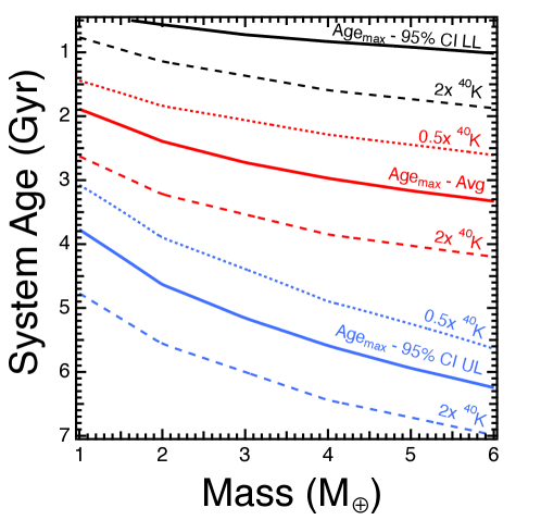
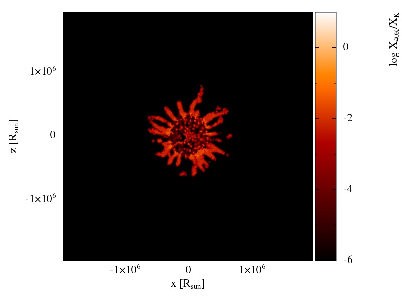
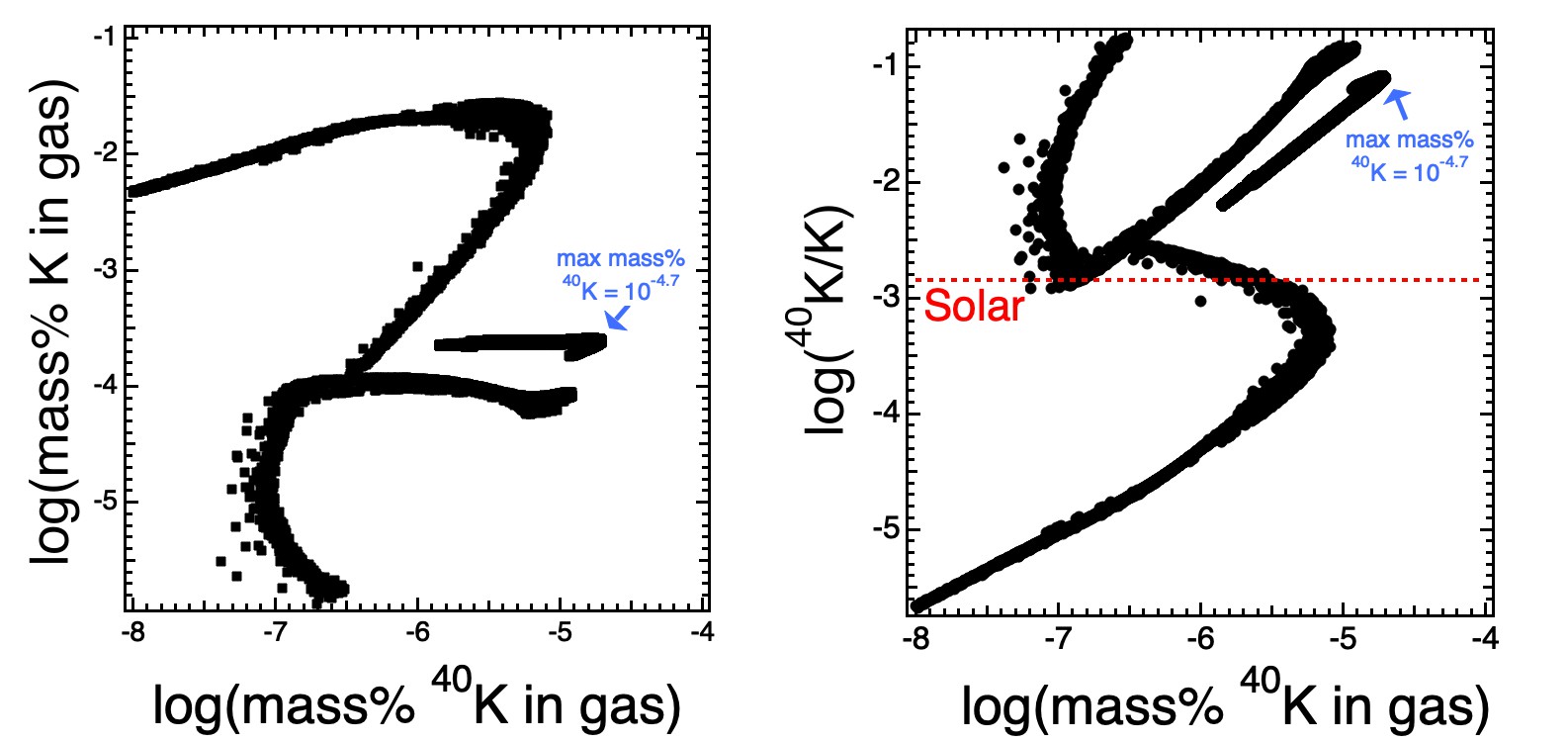
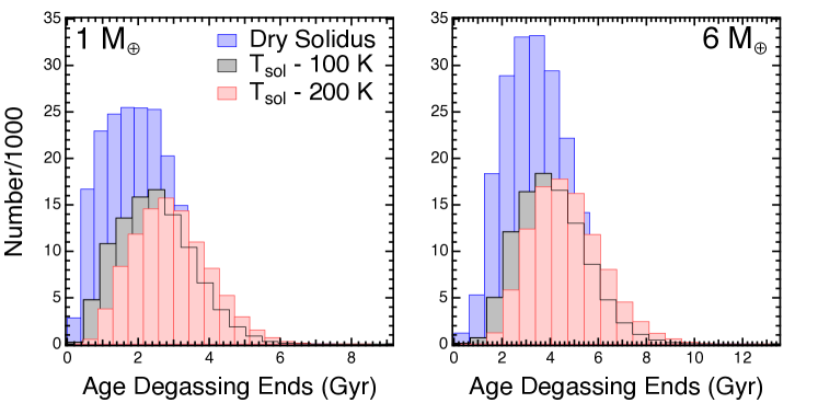

References
- Agol et al. (2021) Agol, E., Dorn, C., Grimm, S. L., et al. 2021, The Planetary Science Journal, 2, 1, doi: 10.3847/PSJ/abd022
- Alexander (2005) Alexander, C. M. O. 2005, Meteoritics & Planetary Science, 40, 943, doi: 10.1111/j.1945-5100.2005.tb00166.x
- Bada & Korenaga (2018) Bada, J. L., & Korenaga, J. 2018, Life, 8, doi: 10.3390/life8040055
- Barbuy et al. (2011) Barbuy, B., Spite, M., Hill, V., et al. 2011, A&A, 534, A60, doi: 10.1051/0004-6361/201117450
- Beattie (1993) Beattie, P. 1993, Nature, 363, 63, doi: 10.1038/363063a0
- Beers & Christlieb (2005) Beers, T. C., & Christlieb, N. 2005, ARA&A, 43, 531, doi: 10.1146/annurev.astro.42.053102.134057
- Botelho et al. (2019) Botelho, R. B., Milone, A. d. C., Meléndez, J., et al. 2019, MNRAS, 482, 1690, doi: 10.1093/mnras/sty2791
- Breuer & Moore (2015) Breuer, D., & Moore, W. 2015, in Treatise on Geophysics (Second Edition), second edition edn., ed. G. Schubert (Oxford: Elsevier), 255 – 305, doi: https://doi.org/10.1016/B978-0-444-53802-4.00173-1
- Burgasser & Mamajek (2017) Burgasser, A. J., & Mamajek, E. E. 2017, ApJ, 845, 110, doi: 10.3847/1538-4357/aa7fea
- Cowan & Abbot (2014) Cowan, N. B., & Abbot, D. S. 2014, Astrophys. J., 781, 27, doi: 10.1088/0004-637X/781/1/27
- Crowley et al. (2011) Crowley, J. W., Gérault, M., & O’Connell, R. J. 2011, EPSL, 310, 380, doi: 10.1016/j.epsl.2011.08.035
- Desch et al. (2020) Desch, S. J., Abbot, D., Krijt, S., et al. 2020, in Planetary Diversity, 2514-3433 (IOP Publishing), 6–1 to 6–40, doi: 10.1088/2514-3433/abb4d9ch6
- Desch et al. (2018) Desch, S. J., Kalyaan, A., & Alexander, C. M. O. 2018, The Astrophysical Journal Supplement Series, 238, 11, doi: 10.3847/1538-4365/aad95f
- Dohm & Maruyama (2015) Dohm, J. M., & Maruyama, S. 2015, Geoscience Frontiers, 6, 95, doi: https://doi.org/10.1016/j.gsf.2014.01.005
- Dorn et al. (2018) Dorn, C., Noack, L., & Rozel, A. B. 2018, Astron. Astrophys., 614, A18, doi: 10.1051/0004-6361/201731513
- Driscoll & Bercovici (2014) Driscoll, P., & Bercovici, D. 2014, Phys. Earth Planet. Inter., 236, 36, doi: 10.1016/j.pepi.2014.08.004
- Duffy et al. (2015) Duffy, T., Madhusudhan, N., & Lee, K. 2015, in Treatise on Geophysics (Second Edition), second edition edn., ed. G. Schubert (Oxford: Elsevier), 149–178, doi: https://doi.org/10.1016/B978-0-444-53802-4.00053-1
- Ellinger et al. (2012) Ellinger, C. I., Young, P. A., Fryer, C. L., & Rockefeller, G. 2012, ApJ, 755, doi: 10.1088/0004-637X/755/2/160
- Fesen & Milisavljevic (2016) Fesen, R. A., & Milisavljevic, D. 2016, ApJ, 818, doi: 10.3847/0004-637X/818/1/17
- Foley (2019) Foley, B. J. 2019, Astrophys. J., 875, 72, doi: 10.3847/1538-4357/ab0f31
- Foley et al. (2020) Foley, B. J., Houser, C., Noack, L., & Tosi, N. 2020, in Planetary Diversity: Rocky Planet Processes and their Observational Signatures, ed. E. J. Tasker, C. Unterborn, M. Laneuville, Y. Fuji, S. J. Desch, & H. E. Hartnett (Bristol, UK: IOP Publishing), 4–1 – 4–60, doi: doi:10.1088/2514-3433/abb4d9ch4
- Foley & Smye (2018a) Foley, B. J., & Smye, A. J. 2018a, Astrobiology, 18, 873, doi: 10.1089/ast.2017.1695
- Foley & Smye (2018b) —. 2018b, Astrobiology, 18, 873, doi: 10.1089/ast.2017.1695
- Fraeman & Korenaga (2010) Fraeman, A. A., & Korenaga, J. 2010, Icarus, 210, 43, doi: 10.1016/j.icarus.2010.06.030
- Frank et al. (2014) Frank, E. A., Meyer, B. S., & Mojzsis, S. J. 2014, Icarus, 243, 274, doi: 10.1016/j.icarus.2014.08.031
- Frebel et al. (2007) Frebel, A., Christlieb, N., Norris, J. E., et al. 2007, Astrophys. J. Lett., 660, L117, doi: 10.1086/518122
- García et al. (2017) García, F., Suárez, A. E., Miceli, M., et al. 2017, A&A, 604, doi: 10.1051/0004-6361/201731418
- Glaser et al. (2020) Glaser, D. M., Hartnett, H. E., Desch, S. J., et al. 2020, ApJ, 893, 163, doi: 10.3847/1538-4357/ab822d
- Goriely & Arnould (2001) Goriely, S., & Arnould, M. 2001, A&A, 379, 1113, doi: 10.1051/0004-6361:20011368
- Grewal et al. (2020) Grewal, D. S., Dasgupta, R., & Farnell, A. 2020, Geochim. Cosmochim. Acta, 280, 281, doi: 10.1016/j.gca.2020.04.023
- Hammer et al. (2010) Hammer, N. J., Janka, H. T., & Müller, E. 2010, ApJ, 714, 1371, doi: 10.1088/0004-637X/714/2/1371
- Hansen et al. (2017) Hansen, T. T., Simon, J. D., Marshall, J. L., et al. 2017, ApJ, 838, 44, doi: 10.3847/1538-4357/aa634a
- Hart & Brooks (1974) Hart, S. E., & Brooks, C. 1974, Geochim. Cosmchim. Acta, 38, 1799, doi: 10.1016/0016-7037(74)90163-X
- Hauck & Phillips (2002) Hauck, S. A., & Phillips, R. J. 2002, J. Geophys. Res. Planets, 107, 6, doi: 10.1029/2001JE001801
- Hauri et al. (2006) Hauri, E. H., Gaetani, G. A., & Green, T. H. 2006, Earth Planet. Sci. Lett., 248, 715, doi: 10.1016/j.epsl.2006.06.014
- Hayashi (1981) Hayashi, C. 1981, Progress of Theoretical Physics Supplement, 70, 35, doi: 10.1143/PTPS.70.35
- Hayworth & Foley (2020) Hayworth, B. P. C., & Foley, B. J. 2020, Astrophys. J. Lett., 902, L10, doi: 10.3847/2041-8213/abb882
- Hinkel et al. (2014) Hinkel, N. R., Timmes, F., Young, P. A., Pagano, M. D., & Turnbull, M. C. 2014, AJ, 148, 54. http://stacks.iop.org/1538-3881/148/i=3/a=54
- Hinkel & Unterborn (2018) Hinkel, N. R., & Unterborn, C. T. 2018, ApJ, 853, 83, doi: 10.3847/1538-4357/aaa5b4
- Hirose et al. (2013) Hirose, K., Labrosse, S., & Hernlund, J. 2013, Annual Review of Earth and Planetary Sciences, 41, 657, doi: 10.1146/annurev-earth-050212-124007
- Hirth & Kohlstedt (2003) Hirth, G., & Kohlstedt, D. 2003, in Subduction Factory Mongraph, ed. J. Eiler, Vol. 138 (Washington, DC: Am. Geophys. Union), 83–105
- Karato & Wu (1993) Karato, S., & Wu, P. 1993, Science, 260, 771, doi: 10.1126/science.260.5109.771
- Katz et al. (2003) Katz, R. F., Spiegelman, M., & Langmuir, C. H. 2003, Geochem., Geophys., Geosyst., 4, 1073, doi: 10.1029/2002GC000433
- Kite et al. (2009) Kite, E. S., Manga, M., & Gaidos, E. 2009, ApJ, 700, 1732, doi: 10.1088/0004-637X/700/2/1732
- Korenaga (2009) Korenaga, J. 2009, Geophys. J. Int., 179, 154, doi: 10.1111/j.1365-246X.2009.04272.x
- Krissansen-Totton & Catling (2017) Krissansen-Totton, J., & Catling, D. C. 2017, Nature Communications, 8, 15423, doi: 10.1038/ncomms15423
- Krissansen-Totton et al. (2021) Krissansen-Totton, J., Galloway, M. L., Wogan, N., Dhaliwal, J. K., & Fortney, J. J. 2021, ApJ, 913, 107, doi: 10.3847/1538-4357/abf560
- Kuchner (2004) Kuchner, M. J. 2004, ApJ, 612, 1147, doi: 10.1086/422577
- Kushiro et al. (1968) Kushiro, I., Syono, Y., & Akimoto, S. 1968, J. Geophys. Res., 73, 6023
- Larsson et al. (2013) Larsson, J., Fransson, C., Kjaer, K., et al. 2013, ApJ, 768, doi: 10.1088/0004-637X/768/1/89
- Leonard et al. (2000) Leonard, D. C., Filippenko, A. V., Barth, A. J., & Matheson, T. 2000, ApJ, 536, 239, doi: 10.1086/308910
- Lodders (2003) Lodders, K. 2003, ApJ, 1220, doi: 10.1086/375492
- Lodders et al. (2009) Lodders, K., Palme, H., & Gail, H. P. 2009, 4.4 Abundances of the elements in the Solar System, Vol. 4B (Berlin, Heidelberg: Springer Berlin Heidelberg), 712–770, doi: 10.1007/978-3-540-88055-4_34
- Marty & Tolstikhin (1998) Marty, B., & Tolstikhin, I. N. 1998, Chem. Geol., 145, 233
- Maruyama et al. (2013) Maruyama, S., Ikoma, M., Genda, H., et al. 2013, Geoscience Frontiers, 4, 141
- McDonough (2003) McDonough, W. F. 2003, Compositional Model for the Earth’s Core (Elsevier), 547–568, doi: 10.1016/b0-08-043751-6/02015-6
- McGovern & Schubert (1989) McGovern, P., & Schubert, G. 1989, Earth and planetary science letters, 96, 27
- Mitrovica & Forte (2004) Mitrovica, J. X., & Forte, A. M. 2004, Earth Planet. Sci. Lett., 225, 177, doi: 10.1016/j.epsl.2004.06.005
- Moranchel-Basurto et al. (2017) Moranchel-Basurto, A., Velázquez, P. F., Giacani, E., et al. 2017, MNRAS, 472, 2117, doi: 10.1093/mnras/stx2086
- Morschhauser et al. (2011) Morschhauser, A., Grott, M., & Breuer, D. 2011, Icarus, 212, 541, doi: 10.1016/j.icarus.2010.12.028
- Noack et al. (2016) Noack, L., Höning, D., Rivoldini, A., et al. 2016, Icarus, 277, 215, doi: 10.1016/j.icarus.2016.05.009
- Ohtani (2019) Ohtani, E. 2019, National Science Review, 7, 224, doi: 10.1093/nsr/nwz071
- Ouellette et al. (2007) Ouellette, N., Desch, S. J., & Hester, J. J. 2007, ApJ, 662, 1268, doi: 10.1086/518102
- Palme & O’Neill (2003) Palme, H., & O’Neill, H. S. C. 2003, Treatise on geochemistry, 2, 1
- Pan et al. (2012) Pan, L., Desch, S. J., Scannapieco, E., & Timmes, F. X. 2012, ApJ, 756, 102, doi: 10.1088/0004-637X/756/1/102
- Raymond et al. (2004) Raymond, S. N., Quinn, T., & Lunine, J. I. 2004, Icarus, 168, 1, doi: 10.1016/j.icarus.2003.11.019
- Reese et al. (1998) Reese, C. C., Solomatov, V. S., & Moresi, L.-N. 1998, J. Geophys. Res., 103, 13643, doi: 10.1029/98JE01047
- Reese et al. (1999) —. 1999, Icarus, 139, 67, doi: 10.1006/icar.1999.6088
- Reese et al. (2007) Reese, C. C., Solomatov, V. S., & Orth, C. P. 2007, J. Geophys. Res. Planets, 112, E04S04, doi: 10.1029/2006JE002782
- Reilly et al. (2017) Reilly, E., Maund, J. R., Baade, D., et al. 2017, MNRAS, 470, 1491, doi: 10.1093/mnras/stx1228
- Roederer et al. (2009) Roederer, I. U., Kratz, K.-L., Frebel, A., et al. 2009, ApJ, 698, 1963, doi: 10.1088/0004-637X/698/2/1963
- Schubert et al. (1979) Schubert, G., Cassen, P., & Young, R. E. 1979, Icarus, 38, 192, doi: 10.1016/0019-1035(79)90178-7
- Shimansky et al. (2003) Shimansky, V. V., Bikmaev, I. F., Galeev, A. I., et al. 2003, Astronomy Reports, 47, 750, doi: 10.1134/1.1611216
- Sleep & Zahnle (2001) Sleep, N., & Zahnle, K. 2001, Journal of Geophysical Research, 106, 1
- Solomatov & Moresi (2000) Solomatov, V. S., & Moresi, L.-N. 2000, J. Geophys. Res., 105, 21795, doi: 10.1029/2000JB900197
- Spaargaren et al. (2020) Spaargaren, R. J., Ballmer, M. D., Bower, D. J., Dorn, C., & Tackley, P. J. 2020, A&A, 643, A44, doi: 10.1051/0004-6361/202037632
- Spohn (1991) Spohn, T. 1991, Icarus, 90, 222, doi: 10.1016/0019-1035(91)90103-Z
- Stevenson et al. (1983) Stevenson, D. J., Spohn, T., & Schubert, G. 1983, Icarus, 54, 466, doi: 10.1016/0019-1035(83)90241-5
- Takahashi & Kushiro (1983) Takahashi, E., & Kushiro, I. 1983, American Mineralogist, 68, 859
- Taylor & McLennan (1985) Taylor, S., & McLennan, S. 1985, The Continental Crust: Its Composition and Evolution (Oxford,UK: Blackwell), 312 pp
- Tosi et al. (2017) Tosi, N., Godolt, M., Stracke, B., et al. 2017, Astron. Astrophys., 605, A71, doi: 10.1051/0004-6361/201730728
- Tosi et al. (2017) Tosi, N., Godolt, M., Stracke, B., et al. 2017, A&A, 605, A71, doi: 10.1051/0004-6361/201730728
- Turcotte & Schubert (2002) Turcotte, D., & Schubert, G. 2002, Geodynamics, 2nd edn. (New York: Cambridge Univ. Press)
- Unterborn et al. (2018) Unterborn, C. T., Desch, S. J., Hinkel, N. R., & Lorenzo, A. 2018, Nature Astronomy, 2, 297, doi: 10.1038/s41550-018-0411-6
- Unterborn et al. (2015) Unterborn, C. T., Johnson, J. A., & Panero, W. R. 2015, Astrophys. J., 806, 139, doi: 10.1088/0004-637X/806/1/139
- Valencia et al. (2006) Valencia, D., O’Connell, R. J., & Sasselov, D. 2006, Icarus, 181, 545, doi: 10.1016/j.icarus.2005.11.021
- Valencia et al. (2007) Valencia, D., O’Connell, R. J., & Sasselov, D. D. 2007, Astrophys. J., 670, L45, doi: 10.1086/524012
- Ward-Duong et al. (2018) Ward-Duong, K., Patience, J., Bulger, J., et al. 2018, AJ, 155, 54, doi: 10.3847/1538-3881/aaa128
- Warren (2016) Warren, J. M. 2016, Lithos, 248, 193, doi: 10.1016/j.lithos.2015.12.023
- Wasson et al. (1988) Wasson, J. T., Kallemeyn, G. W., Runcorn, S. K., Turner, G., & Woolfson, M. M. 1988, Philosophical Transactions of the Royal Society of London. Series A, Mathematical and Physical Sciences, 325, 535, doi: 10.1098/rsta.1988.0066
- Willingale et al. (2002) Willingale, R., Bleeker, J. A. M., van der Heyden, K. J., Kaastra, J. S., & Vink, J. 2002, A&A, 381, 1039, doi: 10.1051/0004-6361:20011614
- Wongwathanarat et al. (2015) Wongwathanarat, A., Müller, E., & Janka, H. T. 2015, A&A, 577, doi: 10.1051/0004-6361/201425025
- Young et al. (2009) Young, P. A., Ellinger, C. I., Arnett, D., Fryer, C. L., & Rockefeller, G. 2009, ApJ, 699, 938, doi: 10.1088/0004-637X/699/2/938
- Zhang et al. (2006) Zhang, H. W., Gehren, T., Butler, K., Shi, J. R., & Zhao, G. 2006, A&A, 457, 645, doi: 10.1051/0004-6361:20064909
- Zhou et al. (2016) Zhou, P., Chen, Y., Safi-Harb, S., et al. 2016, ApJ, 831, doi: 10.3847/0004-637X/831/2/192