A Compositional Approach to Safety-Critical Resilient Control for Systems with Coupled Dynamics

Abstract

Complex, interconnected Cyber-physical Systems (CPS) are increasingly common in applications including smart grids and transportation. Ensuring safety of interconnected systems whose dynamics are coupled is challenging because the effects of faults and attacks in one sub-system can propagate to other sub-systems and lead to safety violations. In this paper, we study the problem of safety-critical control for CPS with coupled dynamics when some sub-systems are subject to failure or attack. We first propose resilient-safety indices (RSIs) for the faulty or compromised sub-systems that bound the worst-case impacts of faulty or compromised sub-systems on a set of specified safety constraints. By incorporating the RSIs, we provide a sufficient condition for the synthesis of control policies in each failure- and attack- free sub-systems. The synthesized control policies compensate for the impacts of the faulty or compromised sub-systems to guarantee safety. We formulate sum-of-square optimization programs to compute the RSIs and the safety-ensuring control policies. We present a case study that applies our proposed approach on the temperature regulation of three coupled rooms. The case study demonstrates that control policies obtained using our algorithm guarantee system’s safety constraints.

I Introduction

Safety is an important property of cyber-physical systems (CPS) in multiple domains including power systems and transportation [1, 2, 3]. Safety violations can potentially cause damage to the system and even endanger human lives [4, 5]. To this end, safety verification and safety-critical control for CPS have been extensively studied [1, 2, 6, 7].

CPS have been shown to be vulnerable to random failures and cyber attacks, which can cause safety violations [4, 5]. To mitigate the impacts of faults and cyber attacks, defending mechanisms and resilient control for CPS have garnered significant research attention [8, 9, 10, 11]. Resilient and safety-critical control can be even more challenging for the class of CPS that are formed by the interconnection of sub-systems [12, 13]. Due to the couplings among the sub-systems, faults and attacks in one sub-system may lead to safety violation in other sub-systems and the overall CPS. For instance, the blackout in India in 2012 was caused by the escalation of a local and small disturbance thorough the interconnections of the power system [14]. Thus, an intelligent adversary can utilize such cascading effects to compromise the controllers and cause maximum-impact safety violations. In addition, the dimension of coupled sub-systems grows with the number of sub-systems, posing a scalability challenge in safety verification and safety-critical control design.

To alleviate the scalability challenge, compositional approaches which decompose the safety constraint over the sub-systems have been proposed [15, 16, 17, 18, 19, 20]. These approaches do not consider the presence of attack. Specifically, compositional approaches to fault-tolerant safety-critical control for coupled CPS has received limited research attention.

In this paper, we aim to develop a compositional approach to safety-critical control for interconnected systems in which some of the sub-systems are faulty or compromised. We consider a class of interconnected systems with the sub-systems’ dynamics being coupled, which we will refer as interconnected system or coupled system interchangeably. We propose two types of resilient-safety indices (RSIs), named as intrinsic resilient-safety index (IRSI) and coupled resilient-safety index (CRSI), using the self- and coupled-dynamics of each sub-system, respectively. The sign and magnitude of RSIs characterize and quantify the impacts of faulty or compromised sub-systems on specified safety constraints. Using the proposed RSIs as well as control barrier functions, we provide conditions and algorithm to design control laws for the remaining sub-systems that are fault- and attack-free. We make the following contributions:

• We define RSIs for the sub-systems that are vulnerable to failure or attack. The IRSI bounds the worst-case impact of the sub-system on safety constraint due to intrinsic/self-dynamics, whereas the CRSI bounds the worst-case impact introduced by the couplings.

• Utilizing the proposed RSIs, we derive the control policies in the fault- and attack-free sub-systems. We prove that our proposed control policies guarantee safety in the presence of faulty or compromised sub-systems.

• We propose an algorithm based on sum-of-squares optimization to compute the RSIs and the safety-ensuring control policy in each fault- and attack-free sub-system independently. We discuss two special cases of linear systems and monotone systems, where computationally efficient methods can be used to estimate the RSIs.

• We present a case study of temperature regulation of interconnected rooms to illustrate our approach. We demonstrate that the control policy obtained using our algorithm maintains the specified safety constraints.

The rest of the paper is organized as follows. Section II presents the related works. Section III presents the system model and formulates the problem. Section IV introduces the indices and presents the condition for safety-ensuring control policies. Section V presents the algorithms for computing the indices and synthesizing the control policies. Section VI contains a case study. Section VII concludes the paper.

II Related Work

Safety-critical CPS are widely seen in real-world applications including power systems [4], robotics [21], and intelligent transportation [5, 22]. In the absence of fault or malicious adversary in the system, safety verification and synthesis have been studied using model checking [23] and deductive verification [24]. Recently, barrier function based approaches, which map the safety constraint to a linear constraint on the control policy, have attracted extensive research attention [1, 6, 7].

The existing safety verification approaches focusing on the overall CPS state space become computationally demanding and even intractable [25, 7] when applied to coupled systems. Compositional approaches, which decompose the safety constraint to those defined over low-dimensional sub-systems, have been proposed [15, 16, 17, 18]. The formulations in [15, 16, 17, 18] do not consider the presence of random failures or malicious attacks.

To address the presence of adversary and random failures in CPS, resilient and fault-tolerant CPS have been studied. Typical approaches include employing defense mechanisms against malicious attacks [26, 11, 27] and designing intrusion tolerant system architectures [28, 29, 30, 31, 32]. For complex interconnected CPS, the adversary can compromise the entire system by intruding into a subset of sub-systems and leveraging the interconnection.

For interconnected CPS under malicious attack, attack detectability is investigated in [33] for linear systems with pair-wise interconnections. How to guarantee safety under malicious attacks for interconnected CPS is not considered in [33]. In [20, 19], safety is achieved for interconnected systems by reconfiguring the control law of each sub-system and the coupling topology among them, assuming that each sub-system is exponentially stable in the absence of coupling. However, reconfiguring the control law and coupling topology may not always be feasible for CPS under malicious attack. In addition, verifying the reconfiguration over all possible interdependencies can be computationally expensive when the system is of large-scale.

III System Model and Problem Formulation

This section presents the system model and our problem formulation. Consider a system $\mathcal{S}$ consisting of a finite set of interconnected sub-systems, denoted as $\{\mathcal{S}_{i}\}_{i=1}^{N}$. Each sub-system $\mathcal{S}_{i}$ has

$$\mathcal{S}_{i}:\dot{x}_{i}= f_{i,slf}(x_{i})+g_{i,slf}(x_{i})u_{i}$$

$$+f_{i,cpl}(x_{i},x_{-i})+g_{i,cpl}(x_{i},x_{-i})u_{i}$$ (1)

where $x_{i}\in\mathbb{R}^{n_{i}}$ is the state of sub-system $\mathcal{S}_{i}$, $x_{-i}\in\mathbb{R}^{n-n_{i}}$ is the state of the other sub-systems excluding $\mathcal{S}_{i}$, $u_{i}\in\mathbb{R}^{r_{i}}$ is the input to the sub-system $\mathcal{S}_{i}$, and $n=\sum_{i=1}^{N}n_{i}$. Functions $f_{i,slf}:\mathbb{R}^{n_{i}}\rightarrow\mathbb{R}^{n_{i}}$, $g_{i,slf}:\mathbb{R}^{n_{i}}\rightarrow\mathbb{R}^{n_{i}\times r_{i}}$, $f_{i,cpl}:\mathbb{R}^{n_{i}}\times\mathbb{R}^{n-n_{i}}\rightarrow\mathbb{R}^{n_{i}}$, and $g_{i,cpl}:\mathbb{R}^{n_{i}}\times\mathbb{R}^{n-n_{i}}\rightarrow\mathbb{R}^{n_{i}\times r_{i}}$ are Lipschitz. Note that functions $f_{i,slf}$ and $g_{i,slf}$ are dependent on the states of sub-system $\mathcal{S}_{i}$ only, and we refer to the term

$$F_{i,slf}(x_{i},u_{i})\triangleq f_{i,slf}(x_{i})+g_{i,slf}(x_{i})u_{i}$$

as the self-dynamics of sub-system $\mathcal{S}_{i}$. Since functions $f_{i,cpl}$ and $g_{i,cpl}$ are jointly determined by the states of $x_{i}$ and those of other sub-systems $x_{-i}$, we refer to

$$F_{i,cpl}(x,u_{i})\triangleq f_{i,cpl}(x_{i},x_{-i})+g_{i,cpl}(x_{i},x_{-i})u_{i}$$

as the coupled-dynamics of sub-system $\mathcal{S}_{i}$. We further assume that the inputs to each sub-systems are bounded as $u_{i}\in\mathcal{U}_{i}$ where $\mathcal{U}_{i}=\prod_{j=1}^{r_{i}}[\underline{u}_{i,j},\overline{u}_{i,j}]$ with $\underline{u}_{i,j}<\overline{u}_{i,j}$. A control policy for sub-system $\mathcal{S}_{i}$ is a function $\mu_{i}:\mathbb{R}^{n}\rightarrow\mathcal{U}_{i}$ that maps from the set of system states to the set of control inputs.

Let $x=[x_{1}^{\top}~{}\cdots~{}x_{N}^{\top}]^{\top}\in\mathbb{R}^{n}$ and $u=[u_{1}^{\top}~{}\cdots~{}u_{N}^{\top}]^{\top}\in\mathbb{R}^{r}$ where $r=\sum_{i=1}^{N}r_{i}$. Then the dynamics of $\mathcal{S}$ can be written as

$$\mathcal{S}:\begin{bmatrix}\dot{x}_{1}\\ \vdots\\ \dot{x}_{N}\end{bmatrix}=\begin{bmatrix}F_{1}(x_{1},x_{-1},u_{1})\\ \vdots\\ F_{N}(x_{N},x_{-N},u_{N})\end{bmatrix}\triangleq F(x,u)$$ (2)

where $F_{i}(x_{i},x_{-i},u_{i})=F_{i,slf}(x_{i},u_{i})+F_{i,cpl}(x,u_{i})$.

We consider that system $\mathcal{S}$ is given $K$ safety constraints for all time $t\geq 0$ where $K\in\mathbb{Z}_{+}$. We suppose each safety constraint is represented as $h^{k}(x)\geq 0$ where $h^{k}:\mathbb{R}^{n}\rightarrow\mathbb{R}$ is a continuously differentiable function for each $k=1,\ldots,K$. We denote the corresponding safety set as $\mathcal{C}$ so that $\mathcal{C}=\cap_{k=1}^{N}\{x\in\mathbb{R}^{n}:h^{k}(x)\geq 0\}$. We assume $\mathcal{C}$ is compact.

Some sub-systems are subject to random failures and malicious attacks. In these scenarios, the actuator of a failed or attacked sub-system $\mathcal{S}_{i}$ does not behave as expected. In the following, we assume that there exists a subset of sub-systems such that they are protected and does not incur random failures or attack. We denote this set of sub-systems as $\{\mathcal{S}_{i}:i\in\mathcal{N}_{1}\}$ where $\mathcal{N}_{1}\subseteq\{1,2,\ldots,N\}$ and refer to them as protected sub-systems. In addition, the set of remaining sub-systems that are subject to random failures and malicious attack is denoted as $\{\mathcal{S}_{i}:i\in\mathcal{N}_{2}\}$ where $\mathcal{N}_{2}\subseteq\{1,\ldots,N\}$ and we to refer them as vulnerable sub-systems. Note, $\mathcal{N}_{1}\cup\mathcal{N}_{2}=\{1,2,\ldots,N\}$ and $\mathcal{N}_{1}\cap\mathcal{N}_{2}=\emptyset$.

Each vulnerable sub-system $\mathcal{S}_{i}$ where $i\in\mathcal{N}_{2}$ may incur fault or cyber attack initiated by a malicious adversary. The fault or attack can alter the control input $u_{i}$ injected to $\mathcal{S}_{i}$ to arbitrary $\tilde{u}_{i}\in\mathcal{U}_{i}$. Since the system is interconnected, the altered behaviors from sub-systems in $\mathcal{N}_{2}$ can further propagate to other protected sub-systems, leading to potential safety violation if the sub-systems in $\mathcal{N}_{1}$ are not properly controlled.

In this paper we aim at computing control policies for the protected sub-systems to ensure safety of system $\mathcal{S}$ irrespective of the states and inputs of the vulnerable sub-systems. We state the problem as follows:

Problem 1.

Consider an interconnected system $\mathcal{S}$ where the sub-systems in $\{\mathcal{S}_{i}:i\in\mathcal{N}_{2}\}$ are subject to failures and malicious attacks while the sub-systems in $\{\mathcal{S}_{i}:i\in\mathcal{N}_{1}\}$ are protected. Synthesize a control policy $\mu_{i}:\mathbb{R}^{n}\rightarrow\mathcal{U}_{i}$ for each $i\in\mathcal{N}_{1}$ such that system $\mathcal{S}$ is safe with respect to $\mathcal{C}$.

IV RSIs and RSI-based Safety Guarantee

In this section, we first propose resilient-safety indices (RSIs) which relate to the worst-case impacts on the safety constraints caused by the self-dynamics and the coupled-dynamics of the vulnerable sub-systems. Based on the RSI we then obtain the sufficient condition for control policies in the protected sub-systems so that safety constraints are guaranteed irrespective of the condition (i.e. whether being faulty/compromised or not) of any of the vulnerable sub-systems.

We first define the RSIs related to the self-dynamics of vulnerable sub-systems $\{\mathcal{S}_{i}:i\in\mathcal{N}_{2}\}$ as follows:

Definition 1.

For each $i\in\mathcal{N}_{2}$ and $k=1,\ldots,K$, we define an intrinsic resilient-safety index (IRSI) of sub-system $\mathcal{S}_{i}$ with respect to function $h^{k}$ as

$$\hat{\gamma}_{i}^{k}=\inf_{x\in\mathcal{C},u_{i}\in\mathcal{U}_{i}}\left\{\frac{\partial h^{k}}{\partial x_{i}}F_{i,slf}(x_{i},u_{i})\right\}$$ (3)

The IRSI $\hat{\gamma}_{i}^{k}$ models the worst-case impact from the self-dynamics of sub-system $\mathcal{S}_{i}$ on the safety constraint $h^{k}(x)\geq 0$. The non-negative value of $\hat{\gamma}_{i}^{k}$ indicates that the sub-system $\mathcal{S}_{i}$ is intrinsically resilient-safe with respect to constraint $h^{k}(x)\geq 0$ as the self-dynamics do not contribute to the safety violation of $h^{k}(x)\geq 0$ for any $u_{i}\in\mathcal{U}_{i}$. The negative value of $\hat{\gamma}_{i}^{k}$ indicates that the self-dynamics of $\mathcal{S}_{i}$ can potentially cause violation to the safety constraint $h^{k}(x)\geq 0$ in the presence of attack or fault (the smaller $\hat{\gamma}_{i}^{k}$ is, the more detrimental $\mathcal{S}_{i}$ intrinsically is in violating $h^{k}(x)\geq 0$).

However, when $\hat{\gamma}_{i}^{k}$ is not available or not easy to compute, we may instead approximate it by finding a bound $\gamma_{i}^{k}\in\mathbb{R}$ such that for all $x\in\mathcal{C}$ and $u_{i}\in\mathcal{U}_{i}$

$$\frac{\partial h^{k}}{\partial x_{i}}F_{i,slf}(x_{i},u_{i})\geq\gamma_{i}^{k}.$$ (4)

By Definition 1, we have $\hat{\gamma}_{i}^{k}\geq\gamma_{i}^{k}$ for any $\gamma_{i}^{k}$ satisfying (4).

Now we define the RSIs related to the coupled-dynamics of vulnerable sub-systems $\{\mathcal{S}_{i}:i\in\mathcal{N}_{2}\}$ as follows:

Definition 2.

For each $k=1,\ldots,K$, we define a coupled resilient-safety index (CRSI) for all vulnerable sub-systems $\mathcal{S}_{i}$ with respect to function $h^{k}$ as

$$\hat{\beta}^{k}=\inf_{x\in\mathcal{C},u_{i}\in\mathcal{U}_{i}}\left\{\sum_{i\in\mathcal{N}_{2}}\frac{\partial h}{\partial x_{i}}F_{i,cpl}(x,u_{i})\right\}$$ (5)

The CRSI $\hat{\beta}^{k}$ models the worst-case impact from coupled dynamics of vulnerable sub-systems on the safety constraint $h^{k}(x)\geq 0$. The non-negative value of $\hat{\beta}^{k}$ indicates that the coupled-dynamics of the vulnerable sub-systems do not contribute to the safety violation of $h^{k}(x)\geq 0$ for any $u_{i}\in\mathcal{U}_{i}$ where $i\in\mathcal{N}_{2}$. The negative value of $\hat{\beta}^{k}$ indicates that the coupled-dynamics of the vulnerable sub-systems can potentially cause violation to the safety constraint $h^{k}(x)\geq 0$ in presence of attack or fault (the smaller $\hat{\beta}^{k}$ is, the more detrimental the coupled-dynamics of the vulnerable sub-systems are in violating $h^{k}(x)\geq 0$).

However, when $\hat{\beta}_{i}^{k}$ is not available or not easy to compute, we may approximate it by finding $\beta^{k}\in\mathbb{R}$ such that for all $x\in\mathcal{C}$ and $u_{i}\in\mathcal{U}_{i}$

$$\sum_{i\in\mathcal{N}_{2}}\frac{\partial h^{k}}{\partial x_{i}}F_{i,cpl}(x,u_{i})\geq\beta^{k}$$ (6)

By Definition 2, we have $\hat{\beta}^{k}\geq\beta^{k}$ for any $\beta^{k}$ satisfying (6).

Next, we present our main result based on the IRSI and CRSI given in Definition 1 and 2. We derive a sufficient condition for control policies in the protected sub-systems such that system $\mathcal{S}$ satisfies all the safety constraints. The result is formalized below.

Theorem 1.

Suppose there exist constants $\alpha_{i}^{k}\in[0,1]$ and a control policy $\mu_{i}:\mathbb{R}^{n}\rightarrow\mathcal{U}_{i}$ for each $i\in\mathcal{N}_{1}$ such that the following holds for all $i\in\mathcal{N}_{1}$ and $k=1,\ldots,K$:

$$\frac{\partial h^{k}}{\partial x_{i}}F_{i}(x_{i},x_{-i},u_{i})\geq\alpha_{i}^{k}\left(-\eta_{i}^{k}(h^{k}(x))-\beta^{k}-\sum_{j\in\mathcal{N}_{2}}\gamma_{j}^{k}\right)$$ (7)

where $\gamma_{j}^{k}$, $\beta^{k}$ are given in Eqn. (4) and (6), $\eta_{i}^{k}$ is an extended class $\mathcal{K}$ function and $\sum_{i\in\mathcal{N}_{1}}\alpha_{i}^{k}=1$ for each $k=1,\ldots,K$. Then the interconnected system $\mathcal{S}$ is safe with respect to $\mathcal{C}$ for all $t\geq 0$ by taking control policy $\mu_{i}$ at each $i\in\mathcal{N}_{1}$ given that $x(0)\in\mathcal{C}$.

Proof.

According to (2) we can compute $\frac{\partial h^{k}}{\partial x}F(x,u)$ for each $k=1,\ldots,K$ as

$$\frac{\partial h^{k}}{\partial x}F(x,u)=\sum_{i=1}^{N}\frac{\partial h^{k}}{\partial x_{i}}F_{i}(x_{i},x_{-i},u_{i})$$

$$= \sum_{i\in\mathcal{N}_{1}}\frac{\partial h^{k}}{\partial x_{i}}F_{i}(x_{i},x_{-i},u_{i})+\sum_{i\in\mathcal{N}_{2}}\frac{\partial h^{k}}{\partial x_{i}}F_{i}(x_{i},x_{-i},u_{i})$$

$$\geq \sum_{i\in\mathcal{N}_{1}}\alpha_{i}^{k}[-\eta_{i}^{k}(h^{k}(x))-\beta^{k}-\sum_{j\in\mathcal{N}_{2}}\gamma_{j}^{k}]$$

$$\quad+\sum_{i\in\mathcal{N}_{2}}\frac{\partial h^{k}}{\partial x_{i}}[F_{i,slf}(x_{i},u_{i})+F_{i,cpl}(x_{i},u_{i})]$$

$$= -\sum_{i\in\mathcal{N}_{1}}\alpha_{i}^{k}\eta_{i}^{k}(h^{k}(x))+\sum_{i\in\mathcal{N}_{2}}\Big{(}\frac{\partial h^{k}}{\partial x_{i}}F_{i,slf}(x_{i},u_{i})-\gamma_{i}^{k}\Big{)}$$

$$\quad\quad+\Big{(}\sum_{i\in\mathcal{N}_{2}}\frac{\partial h^{k}}{\partial x_{i}}F_{i,cpl}(x_{i},,u_{i})-\beta^{k}\Big{)}$$

$$\geq -\sum_{i\in\mathcal{N}_{1}}\alpha_{i}^{k}\eta_{i}^{k}(h^{k}(x))$$

where the last inequality holds by Eqn. (4) and (6). Since that $\eta_{i}^{k}$ is an extended class $\mathcal{K}$ function and $\alpha_{i}^{k}\in[0,1]$, we have that $\sum_{i\in\mathcal{N}_{1}}\alpha_{i}^{k}\eta_{i}^{k}$ is also an extended class $\mathcal{K}$ function. Thus $\frac{\partial h^{k}}{\partial x}F(x,u)\geq-\eta^{k}(h^{k}(x))$. Using the property of control barrier function [1] and the assumption that $x(0)\in\mathcal{C}$, we have that the coupled system satisfies that $h^{k}(x)\geq 0$ for all $k=1,\dots,K$ and $t\geq 0$. Therefore we have that system $\mathcal{S}$ is safe with respect to $\mathcal{C}$. ∎

In Theorem 1, constant $\alpha_{i}^{k}$ specifies the weight on each protected sub-system $\mathcal{S}_{i}$ to satisfy the safety constraint $h^{k}(x)\geq 0$. For example, $\alpha_{i}^{k}=1$ means that we let sub-system $\mathcal{S}_{i}$ be solely responsible for maintaining safety constraint $h^{k}(x)\geq 0$ among all the protected sub-systems. Parameter $\alpha_{i}^{k}$ for $i=1,\ldots,m$ and $k=1,\ldots,K$ are chosen in a way so that the condition (7) is satisfied.

Theorem 1 implies that if the approximated RSIs $\gamma_{i}^{k}$ and $\beta^{k}$ for the vulnerable sub-systems are known, then the control policies in the protected sub-systems that guarantee system’s safety can be calculated without knowing the exact models of the vulnerable sub-systems. This is useful since the control input $\tilde{u}_{i}$ employed in a sub-system compromised by adversarial attack is usually unknown. However, from Theorem 1, it is clear that one should use true values of RSIs, i.e., $\hat{\gamma}_{i}^{k}$ and $\hat{\beta}^{k}$ as $\gamma_{i}^{k}$ and $\beta^{k}$ so that condition (7) is less restrictive. RSIs or their approximations can be computed either numerically or analytically. Below we present a simple example for which we find the closed-form expressions for $\gamma_{i}^{k}$ and $\beta^{k}$. This will help us to gain some insights on RSIs.

Example: Consider a system $\mathcal{S}:\dot{x}=Ax+Bu$ where

$$A=\begin{bmatrix}a_{11}&\ldots&a_{1N}\\ \vdots&\ddots&\vdots\\ a_{N1}&\ldots&a_{NN}\end{bmatrix},\quad B=\begin{bmatrix}b_{11}&\ldots&0\\ \vdots&\ddots&\vdots\\ 0&\ldots&b_{NN}\end{bmatrix}$$

Here $A\in\mathbb{R}^{N\times N}$, $B\in\mathbb{R}^{N\times N}$, $x=[x_{1}\ldots x_{N}]^{\top}\in\mathbb{R}^{n}$ and $u=[u_{1}\ldots u_{N}]^{\top}$. Matrix $A$ represents the system matrix for a synchronization dynamics with $a_{ii}=-\sum_{j=1,j\neq i}^{N}a_{ij}<0$. We consider that the system is given one ellipsoid safety constraint $\mathcal{C}=\{x\in\mathbb{R}^{N}:h(x)\geq 0\}$ where $h(x)=1-\sum_{i=1}^{N}c_{i}x_{i}^{2}$ and $c_{i}>0$. Let the constraints on input be $\mathcal{U}_{i}\in[-1,1]$. Let $\mathcal{N}_{1}=\{1,\ldots,m\}$ and $\mathcal{N}_{2}=\{m+1,\ldots,N\}$. Then, we can write

$$\frac{\partial h}{\partial x_{i}}F_{i,slf}(x_{i},u_{i})=-2c_{i}x_{i}(a_{ii}x_{i}+b_{ii}u_{i})$$

$$\quad\quad=-2c_{i}a_{ii}(x_{i}+\frac{b_{ii}u_{i}}{2a_{ii}})^{2}+\frac{b_{ii}^{2}c_{i}u_{i}^{2}}{2a_{ii}}$$

$$\beta=\sum_{i=m+1}^{N}\big{(}-2c_{i}x_{i}\sum_{j=1,j\neq i}^{N}(a_{ij}x_{j})\big{)}$$

$$\quad\quad\geq\sum_{i=m+1}^{N}2c_{i}|a_{ii}|~{}\min_{x\in\mathcal{C}}(x_{i}x_{j})$$

Then with some efforts it can be shown that $\gamma_{i}=-\frac{b_{ii}^{2}c_{i}}{2|a_{ii}|}$ and $\beta=-\frac{c_{\mathcal{N}_{2}}^{max}}{c^{min}}\sum_{i=m+1}^{N}|a_{ii}|$ satisfy the conditions (4) and (6) respectively where $c_{\mathcal{N}_{2}}^{max}$ is the maximum value in $\{c_{m+1},\ldots c_{N}\}$ and $c^{min}$ is the minimum value in $\{c_{1},\ldots,c_{N}\}$. The expression of $\gamma_{i}$ implies that $\gamma_{i}$ is inversely related to the magnitude of the eigenvalue of the self-dynamics of that sub-system $\mathcal{S}_{i}$ (i.e. the higher the magnitude of eigenvalue or faster decreasing the dynamics, the lower $\gamma_{i}$). This indicates that a sub-system with fast decreasing self-dynamics plays less significant role in violating the safety constraint under fault or attack. Now, the expression of $\beta$ implies that the higher the coupling (i.e. $|a_{ii}|=|\sum_{j=1,j\neq i}^{N}a_{ij}|$ for $i\in\mathcal{N}_{2}$), the higher the magnitude of $\beta$ becomes. Therefore, the sub-systems that have higher couplings will be critical in violating the safety constraint under fault or attack.

V Algorithmic computation of RSIs and control policies

In this section we present algorithms to compute the control policies and associated RSIs i.e. $\gamma_{i}^{k}$ and $\beta_{k}$. Our proposed algorithms are based on sum-of-squares (SOS) optimization. Later, we present two special classes of systems for which RSIs can be computed more efficiently.

In the remainder of this section, we make the following assumption on the system dynamics and the given safety constraints.

Assumption 1.

We assume that $F(x,u)$ is polynomial in $x$ and $u$, and $h^{k}(x)$ is polynomial in $x$ for $k=1,\ldots,K$ respectively.

Based on the above assumption, we now aim to compute IRSI $\hat{\gamma}_{i}^{k}$ and CRSI $\hat{\beta}^{k}$ using SOS optimization. However, in general IRSI and CRSI are difficult to compute. Therefore we relax the condition and focus on finding approximated values of IRSI and CRSI. Specifically, we find $\gamma_{i}^{k}$ and $\beta^{k}$ so that inequalities (4) and (6) are reasonably tight. For that we first show how to translate conditions (4) and (6) into SOS constraints. Then we minimize $\gamma_{i}^{k}$ and $\beta^{k}$ in the SOS formulation to make (4) and (6) reasonably tight.

Following results formalize our computation method of $\gamma_{i}^{k}$ for each $i\in\mathcal{N}_{2}$ and $k\in\{1,\ldots,K\}$.

Lemma 1.

Suppose Assumption 1 holds and $p_{s}(x,u_{i})$, $w_{j}(x,u_{i})$ and $v_{j}(x,u_{i})$ are SOS polynomials where $j=1,2,\ldots,r_{i}$ and $s=1,\ldots,K$. For $i\in\mathcal{N}_{2}$ and $k\in\{1,\ldots,K\}$ if $\gamma_{i}^{k}$ is the solution to the sum-of-squares program:

$$\min_{\gamma_{i}^{k}}~{}-\gamma_{i}^{k}$$ (8a)

$$\text{s.t.}\frac{\partial h^{k}}{\partial x_{i}}F_{i,slf}(x_{i},u_{i})-\gamma_{i}^{k}-\sum_{s=1}^{k}p_{s}(x,u_{i})h^{s}(x)$$

$$\quad-\sum_{j=1}^{r_{i}}\big{(}w_{j}(x,u_{i})(u_{i,j}-\underline{u}_{i,j})+v_{j}(x,u_{i})(\overline{u}_{i,j}-u_{i,j})\big{)}$$

is SOS (8b)

then $\gamma_{i}^{k}$ satisfies Eqn. (4). Furthermore $\gamma_{i}^{k}=\hat{\gamma}_{i}^{k}$ when expressions in (8b) is quadratic.

Proof.

Let $\gamma_{i}^{k}$ be the solution to SOS program (8). Since $p_{s}(x,u_{i})$, $w_{j}(x,u_{i})$ and $v_{j}(x,u_{i})$ are SOS polynomials, we have that $\sum_{s=1}^{k}p_{s}(x,u_{i})h^{s}(x)\geq 0$ for all $x\in\mathcal{C}$ and $\sum_{j=1}^{r_{i}}\big{(}w_{j}(x,u_{i})(u_{i,j}-\underline{u}_{i,j})+v_{j}(x,u_{i})(\overline{u}_{i,j}-u_{i,j}))\geq 0$ for all $u_{i}\in\mathcal{U}_{i}$. Thus any $\gamma_{i}^{k}$ rendering constraint (8b) an SOS satisfies that

$$\frac{\partial h^{k}}{\partial x_{i}}F_{i,slf}(x_{i},u_{i})\geq\gamma_{i}^{k},~{}\forall x\in\mathcal{C},u_{i}\in\mathcal{U}_{i}$$

Now suppose the case when expressions in (8b) is quadratic. Assume that $\gamma_{i}^{k}\neq\hat{\gamma}_{i}^{k}$. Then $\hat{\gamma}_{i}^{k}>\gamma_{i}^{k}$ by the definition of $\hat{\gamma}_{i}^{k}$. Since for quadratic polynomial SOS and non-negativity is equivalent [34], $\hat{\gamma}_{i}^{k}$ is also feasible to constraint (8b). However, this contradicts the optimality of $\gamma_{i}^{k}$ to SOS program (8). Hence $\gamma_{i}^{k}=\hat{\gamma}_{i}^{k}$ in this case. ∎

Similarly we use the following result to compute $\beta^{k}$ for each $k\in\{1,\ldots,K\}$.

Lemma 2.

Suppose Assumption 1 holds and $p_{s}(x,u_{i})$, $w_{i,j}(x,u)$ and $v_{i,j}(x,u)$ are SOS polynomials where $i\in\mathcal{N}_{2}$, $j=1,2,\ldots,r_{i}$ and $s=1,\ldots,K$. For $k\in\{1,\ldots,K\}$ if $\beta^{k}$ is the solution to the sum-of-squares program:

$$\min_{\beta^{k}}~{}-\beta^{k}$$ (9a)

$$\text{s.t.}\sum_{i\in\mathcal{N}_{2}}\frac{\partial h^{k}}{\partial x_{i}}F_{i,cpl}(x,u_{i})-\beta^{k}-\sum_{s=1}^{k}p_{s}(x,u_{i})h^{s}(x)$$

$$\quad\quad-\sum_{i\in\mathcal{N}_{2}}\sum_{j=1}^{r_{i}}\big{(}w_{i,j}(x,u)(u_{i,j}-\underline{u}_{i,j})$$

$$\quad\quad+v_{i,j}(x,u)(\overline{u}_{i,j}-u_{i,j})\big{)}\text{ is SOS}$$ (9b)

then $\beta^{k}$ satisfies Eqn. (6). Furthermore $\beta^{k}=\hat{\beta}^{k}$ when expressions in (9b) is quadratic.

Proof.

Let $\beta^{k}$ be the solution to SOS program (9). Since $p_{s}(x,u)$, $w_{i,j}(x,u)$ and $v_{i,j}(x,u)$ are SOS polynomials, we have that $\sum_{s=1}^{k}p_{s}(x,u_{i})h^{s}(x)\geq 0$ for all $x\in\mathcal{C}$ and $\sum_{i\in\mathcal{N}_{2}}\sum_{j=1}^{r_{i}}\big{(}w_{i,j}(x,u)(u_{i,j}-\underline{u}_{i,j})+v_{i,j}(x,u)(\overline{u}_{i,j}-u_{i,j})\big{)}$ for all $u_{i}\in\mathcal{U}_{i}$ and $i\in\mathcal{N}_{2}$. Thus $\beta^{k}$ satisfies that

$$\sum_{i\in\mathcal{N}_{2}}\frac{\partial h^{k}}{\partial x_{i}}F_{i,cpl}(x,u_{i})\geq\beta^{k},~{}\forall x\in\mathcal{C},u_{i}\in\mathcal{U}_{i},i\in\mathcal{N}_{2}$$

We note that $\beta^{k}=\hat{\beta}^{k}$ when expressions in (9b) is quadratic using arguments similar to the proof of Lemma 1. ∎

Now we present our algorithm for computing control policies given the approximated IRSI and CRSI, i.e. $\gamma_{i}^{k}$ and $\beta^{k}$. To do so, we translate the condition given in (7) as SOS constraint and formulate an SOS program to compute the control input $u_{i}$ for each $i\in\mathcal{N}_{1}$. The following lemma presents the result.

Lemma 3.

Suppose $\gamma_{i}^{k}$ and $\beta^{k}$ are given for each $i\in\mathcal{N}_{2}$ and $k\in\{1,\ldots,K\}$. Suppose the following expressions are SOS for each $i\in\mathcal{N}_{1}$ and $k\in\{1,\ldots,K\}$.

$$\frac{\partial h^{k}}{\partial x_{i}}[f_{i,slf}(x_{i})+g_{i,slf}(x_{i})\tau_{i}(x)+f_{i,cpl}(x_{i},x_{-i})$$

$$\quad+g_{i,cpl}(x_{i},x_{-i})\tau_{i}(x)]-\alpha_{i}^{k}\Big{(}-\eta_{i}^{k}(h^{k}(x))-\beta^{k}$$

$$\quad\quad-\sum_{j\in\mathcal{N}_{2}}\gamma_{j}^{k}\Big{)}-\sum_{s=1}^{K}\lambda_{s}(x)h^{s}(x),$$ (10a)

$$\tau_{i,j}(x)-\underline{u}_{i,j},\quad\overline{u}_{i,j}-\tau_{i,j}(x),~{}\forall j=1,\ldots,r_{i},$$ (10b)

where $\lambda_{s}(x)$ is an SOS polynomial and $\tau_{i,j}(x)$ is a polynomial in $x$ for $i\in\mathcal{N}_{1}$, $j=1,\ldots,r_{i}$ and $s=1,\ldots,K$. Then condition (7) is satisfied for $x\in\mathcal{C}$ when $u_{i}$ is chosen as $u_{i}=\tau_{i}(x)=[\tau_{i,1}(x)\cdots\tau_{i,r_{i}}(x)]^{T}$ for all $i\in\mathcal{N}_{1}$.

Proof.

Since $\lambda_{s}(x)$ is an SOS polynomial, we have that $\lambda_{s}(x)h^{s}(x)\geq 0$ implying $\sum_{s=1}^{K}\lambda_{s}(x)h^{s}(x)\geq 0$ for all $x\in\mathcal{C}$. When Eqn. (10) is an SOS, we thus have that

$$\frac{\partial h^{k}}{\partial x_{i}}F_{i,slf}(x_{i},\tau_{i}(x))+F_{i,cpl}(x,\tau_{i}(x))\\ -\alpha_{i}^{k}\Big{(}-\eta_{i}^{k}(h^{k}(x))-\beta^{k}-\sum_{j\in\mathcal{N}_{2}}\gamma_{j}^{k}\Big{)}\geq 0$$ (11)

holds for all $x\in\mathcal{C}$. By choosing $u_{i}=\tau_{i}(x)$ for all $i\in\mathcal{N}_{1}$, we recover the condition in Eqn. (7). ∎

Algorithm 1 Solution algorithm for finding control policy

1:Input: Dynamics $F$. Functions $\{h^{k}\}_{k=1}^{K}$. Constants $\{\alpha_{i}^{k}\},\{\underline{u}_{i,j}\},\{\overline{u}_{i,j}\}$.

2:Output: $\{\gamma_{i}^{k}\}_{i\in\mathcal{N}_{2}}$, $\beta^{k}$, and control inputs $\{u_{i}\}$.

3:Solve the SOS programs in Eqn. (8) and (9) to calculate $\gamma_{i}^{k}$ and $\beta^{k}$ for each for each $i\in\mathcal{N}_{2}$ and $k\in\{1,\ldots,K\}$.

4:Initialization: $Flag\leftarrow 1$.

5:for $i\in\mathcal{N}_{1}$ do

6:     Solve (10) using $\gamma_{i}^{k}$ and $\beta^{k}$ for all $k=1,\ldots K$.

7:     if Line 6 is feasible then

8:         $u_{i}\leftarrow\tau_{i}$.

9:     else

10:         $Flag\leftarrow 0$.

11:         break

12:     end if

13:end for

14:if $Flag=1$ then

15:     return $\{\gamma_{i}^{k}\}$, $\{\beta^{k}\}$ and $\{u_{i}\}$.

16:else

17:     Not feasible.

18:end if

Now we present Algorithm 1 that uses the above results to find the control policies in the protected sub-systems. First the approximated RSIs $\gamma_{i}^{k}$ and $\beta^{k}$ are calculated using Lemma 1 and 2 for each vulnerable sub-system and safety constraint. Then control policy $\mu_{i}$ for each $i\in\mathcal{N}_{1}$ is calculated from line 5 to line 12. If the SOS conditions in Eqn. (10) is feasible for all $i\in\mathcal{N}_{1}$ and $k\in\{1,\ldots K\}$, the algorithm returns the control policies for all the protected sub-systems. We remark that Algorithm 1 can be implemented in an offline manner and it can calculate the control policy for each protected sub-system in parallel.

It may be possible that there exists no control policy that guarantees safety of the system depending on the cardinality of $\mathcal{N}_{1}$ or the ranges of $\mathcal{U}$ and $\mathcal{C}$ or the model dynamics $F(x,u)$. In that case Algorithm 1 becomes infeasible, i.e. fails to find feasible control policies that guarantee safety. However, it may happen that Algorithm 1 is infeasible for $\mathcal{C}$ but feasible for some set $\tilde{\mathcal{C}}\subset\mathcal{C}$. In such scenario one need to modify the algorithm and search for the set $\tilde{\mathcal{C}}$ such that the algorithm becomes feasible. In that case the system $\mathcal{S}$ will maintain safety for all $t\geq 0$ if $x(0)\in\tilde{\mathcal{C}}$.

Here we make a remark on the case when any of the safety constraints is local to a sub-system. Suppose there exist $\tilde{k}\in\{1,\ldots,k\}$ and $\tilde{i}\in\{1,\ldots,N\}$ such that $h^{\tilde{k}}:\mathbb{R}^{n_{\tilde{i}}}\rightarrow\mathbb{R}$ is local to sub-system $\mathcal{S}_{\tilde{i}}$ which can be written as $h^{\tilde{k}}(x_{\tilde{i}})$. This implies $\frac{\partial h^{\tilde{k}}}{\partial x_{j}}$ is a vector with all entries being zero for $j\neq\tilde{i}$. If $\tilde{i}\in\mathcal{N}_{1}$, then we have $\sum_{j\in\mathcal{N}_{2}}\hat{\gamma}_{j}^{\tilde{k}}=\hat{\beta}^{\tilde{k}}=0$. This implies $|\mathcal{N}_{1}|-1$ conditions in Theorem 1 are trivially satisfied and can be omitted from the SOS program. However, if $\tilde{i}\in\mathcal{N}_{2}$, then our approach can be modified to obtain less conservative SOS formulation. In this case, instead of calculating $\gamma_{\tilde{i}}^{\tilde{k}}$ (note, $\hat{\gamma}_{j}^{\tilde{k}}=0$ for $j\neq{\tilde{i}}$) and $\beta^{\tilde{k}}$, we can impose the following constraint directly in each of the SOS program: $\frac{\partial h^{\tilde{k}}}{\partial x_{\tilde{i}}}F_{\tilde{i}}(x_{\tilde{i}},x_{-{\tilde{i}}},u_{\tilde{i}})\geq-\eta_{\tilde{i}}^{\tilde{k}}(h^{\tilde{k}}(x_{\tilde{i}}))$ for all $x\in\mathcal{C}$ and $u_{\tilde{i}}\in\mathcal{U}_{\tilde{i}}$. This condition is less conservative than the constraint $\gamma_{\tilde{i}}^{\tilde{k}}+\beta^{\tilde{k}}\geq-\eta_{\tilde{i}}^{\tilde{k}}(h^{\tilde{k}}(x_{\tilde{i}}))$ obtained via Theorem 1. We note that $\frac{\partial h^{\tilde{k}}}{\partial x_{\tilde{i}}}F_{\tilde{i}}(x_{\tilde{i}},x_{-{\tilde{i}}},u_{\tilde{i}})\geq-\eta_{\tilde{i}}^{\tilde{k}}(h^{\tilde{k}}(x_{\tilde{i}}))$ introduces infeasibility if the impact of compromised $u_{\tilde{i}}\in\mathcal{U}_{\tilde{i}}$ on $h^{\tilde{k}}(x_{\tilde{i}})$ cannot be compensated by the system states. For an example see Section VI.

Now we present two special cases where the IRSI $\hat{\gamma}_{i}^{k}$ and CRSI $\hat{\beta}^{k}$ can be obtained more efficiently relative to SOS approach.

V-1 LTI System with Half-Plane Constraint

Consider system $\mathcal{S}$ be given as

$$\mathcal{S}:\dot{x}=Ax+Bu,$$ (12)

where

$$A=\begin{bmatrix}A_{11}&\ldots&A_{1N}\\ \vdots&\ddots&\vdots\\ A_{N1}&\ldots&A_{NN}\end{bmatrix},\quad B=\begin{bmatrix}B_{11}&\ldots&\mathbf{0}\\ \vdots&\ddots&\vdots\\ \mathbf{0}&\ldots&B_{NN}\end{bmatrix}$$

$A_{ij}\in\mathbb{R}^{n_{i}\times n_{j}}$, and $B_{ii}\in\mathbb{R}^{n_{i}\times r_{i}}$. We consider $h^{k}(x)=a_{k}^{\top}x$ where $a_{k}\in\mathbb{R}^{n}$ for all $k=1,\ldots,K$ and set $\mathcal{C}$ is compact. We show that IRSI $\hat{\gamma}_{i}^{k}$ can be computed using a linear program when $\mathcal{U}_{i}=\{u_{i}:w^{\top}u_{i}\geq 0\}$. For each $i\in\mathcal{N}_{2}$, if $\gamma_{i}^{k}=a_{k}^{\top}F_{i,slf}(x_{i}^{*},u_{i}^{*})$, where $(x_{i}^{*},u_{i}^{*})$ is the solution to the following linear program:

$$\min_{x_{i},u_{i}}~{} a_{k}^{\top}F_{i,slf}(x_{i},u_{i})$$ (13a)

s.t. $$a_{k}^{\top}x\geq 0,~{}\forall k$$ (13b)

$$w^{\top}u_{i}\geq 0$$ (13c)

then $\gamma_{i}^{k}=\hat{\gamma}_{i}^{k}$ as given in Definition 1. Let $\mathcal{P}$ be the polyhedron induced by the constraints in Eqn. (13). We have that $\hat{\gamma}_{i}^{k}$ is attained at some vertex of $\mathcal{P}$. Similarly we can consider the computation of CRSI $\hat{\beta}^{k}$. For each sub-system $i\in\mathcal{N}_{2}$, if $\beta^{k}=\sum_{i\in\mathcal{N}_{2}}a_{k}^{\top}F_{i,cpl}(x^{*},u_{i}^{*})$, where $[x^{*},u_{i}^{*}]$ is the solution to the following linear program:

$$\min_{x,u_{i}}~{} \sum_{i\in\mathcal{N}_{2}}a_{k}^{\top}F_{i,cpl}(x,u_{i})$$ (14a)

s.t. $$a_{k}^{\top}x\geq 0,~{}\forall k$$ (14b)

$$w^{\top}u_{i}\geq 0$$ (14c)

then $\beta^{k}=\hat{\beta}^{k}$ as given in Definition 2.

V-2 Monotone System with Hyperrectangle Constraints

In the following, we consider monotone systems under hyperrectangle constraints. Consider system (2) and a safety set $\mathcal{C}=[\underline{x},\overline{x}]$, where $\underline{x},\overline{x}\in\mathbb{R}^{n}$. We consider $\underline{x}\leq\overline{x}$ element-wise, and thus $\mathcal{C}$ is a hyperrectangle.

Definition 3 (Monotonicity [35]).

Function $F(x,u)$ is monotone with respect to $x$ and $u$ if

$$x\leq x^{\prime}\text{ and }u\leq u^{\prime}\implies F(x,u)\leq F(x^{\prime},u^{\prime})$$ (15)

where the order relation $\leq$ is compared element-wise.

Monotonicity of a function $F(x,u)$ can be shown by verifying the signs of $\frac{\partial F}{\partial x}$ and $\frac{\partial F}{\partial u}$ [35]. Using Definition 3, Eqn. (4) and (6), we have the following result:

Lemma 4.

Consider system (2) and a hyperrectangle safety set $\mathcal{C}=[\underline{x},\overline{x}]$. If functions $\tilde{F}_{i,slf}(x,u_{i})=\frac{\partial h^{k}}{\partial x_{i}}F_{i,slf}(x_{i},u_{i})$ and $\tilde{F}_{i,cpl}(x,u_{i})=\frac{\partial h^{k}}{\partial x_{i}}F_{i,cpl}(x,u_{i})$ are monotone with respect to $x$ and $u$ as given in Definition 3, then for $i\in\mathcal{N}_{2}$ and $k=1,\ldots,K$ we have

$$\hat{\gamma}_{i}^{k}=\tilde{F}_{i,slf}(\underline{x},\underline{u}_{i}),$$

$$\hat{\beta}^{k}=\sum_{i\in\mathcal{N}_{2}}\tilde{F}_{i,cpl}(\underline{x},\underline{u}_{i}).$$

VI Case Study

In this section, we illustrate our proposed approach using an example on the temperature regulation in a circular building consisting of $N$ rooms [36]. For each room $i=1,\ldots,N$, we denote its temperature as $x_{i}$ which follows dynamics given as

$$\dot{x}_{i}=\frac{1}{\delta}(w(x_{i+1}+x_{i-1}-2x_{i})+y(T_{e}-x_{i})+z(T_{h}-x_{i})u_{i}),$$ (16)

where $x_{i+1}$ and $x_{i-1}$ are the temperatures of the neighboring rooms, $T_{e}$ is the outside temperature, and $T_{h}$ is the heater temperature. For rooms $i=1$ and $i=N$, we let $x_{0}=x_{N}$ and $x_{N+1}=x_{1}$. In this case study, we consider $N=3$, $T_{e}=-1^{\circ}C$, and $T_{h}=50^{\circ}C$. We additionally let $\mathcal{U}_{1}\in[0,0.6]$ and $\mathcal{U}_{2},\mathcal{U}_{3}\in[-2,2]$. The coefficients $w$, $y$, and $z$ are chosen as $w=0.45$, $y=0.045$, and $z=0.09$, respectively. Parameter $\delta$ is set as $\delta=0.1$. We consider that the controller of room $1$ is compromised via an adversarial attack. Rooms $2$ and $3$ are the protected sub-systems. In the remainder of this section, we study two scenarios.

In the first scenario, we consider that the system is given one safety constraint $x\in\mathcal{C}$ for all time $t\geq 0$, where $\mathcal{C}=\{x:h(x)\geq 0\}$ and

$$h(x)=\left(\frac{\sum_{i=1}^{3}x_{i}}{3}-15\right)\left(20-\frac{\sum_{i=1}^{3}x_{i}}{3}\right).$$

Using the SOS program in Eqn. (8) and (9), we compute the approximated IRSI and CRSI. We have that $\gamma_{1}=-22.05$ and $\beta_{1}=-2.636$. We then synthesize the control input by enforcing constraint (10). We show the average temperature $\frac{\sum_{i=1}^{3}x_{i}}{3}$ at each time step in Fig. 1. We observe that $\frac{\sum_{i=1}^{3}x_{i}}{3}\in[15,20]$ for all time steps and thus $h(x)\geq 0$ for all time.

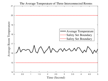
Figure 1: The average temperature of three rooms over $50$ time steps. Room $1$ is compromised and rooms $2,3$ are protected from failure and attack. The average temperature is depicted using solid black line. The boundaries of set $\mathcal{C}$ are shown using red dotted lines.

In the second scenario, we consider a safety set $\mathcal{C}=\{x:h^{i}(x_{i})\geq 0,i=1,2,3\}$. Each function $h^{i}$ specifies a range for the temperature in room $i$. We consider

$$h^{1}(x_{1}) =(16-x_{1})(x_{1}-10),$$

$$h^{2}(x_{2}) =(22-x_{2})(x_{2}-15),$$

$$h^{3}(x_{3}) =(25-x_{3})(x_{3}-14).$$

Since room $1$ is compromised, we can only satisfy the safety constraint $h_{1}$ by regulating the temperature of rooms $2$ and $3$ and utilizing the coupling term $w(x_{2}+x_{3}-2x_{1})$. To ensure the satisfaction of $h^{1}(x_{1})\geq 0$, we introduce the following constraint over $x_{2}$ and $x_{3}$ when synthesizing the control policies for rooms $2$ and $3$:

$$-\frac{\partial h^{1}}{\partial x_{1}}\left[\frac{1}{\delta}(2wx_{1}+yx_{1}-z(T_{h}-x_{1})u_{1})\right]-\eta^{1}(h^{1}(x_{1}))\\ \leq\frac{\partial h^{1}}{\partial x_{1}}\left[\frac{1}{\delta}(w(x_{2}+x_{3})+yT_{e})\right]$$ (17)

where $\eta^{1}(\cdot)$ is a class $\mathcal{K}$ function. When $x_{2}$ and $x_{3}$ are chosen such that constraint (17) is met regardless of $u_{1}$ for any $x_{1}\in[10,16]$, we have that $h^{1}(x_{1})\geq 0$ is satisfied. To this end, we let $u_{1}$ be chosen as the worst-case one with different values of $x_{1}$. By imposing inequality (17) as an additional constraint when synthesizing $u_{2}$ and $u_{3}$, we can guarantee the satisfaction of the safety constraint $x\in\mathcal{C}$, even though room $1$ is compromised. We remark that constraint (17) needs to be compatible with constraints $h^{2}(x_{2})\geq 0$ and $h^{3}(x_{3})\geq 0$ to guarantee the feasibilities of $u_{2}$ and $u_{3}$. One can verify that when $u_{1}\geq 6.2498$, incorporating constraint (17) leads to infeasibility when synthesizing $u_{2}$ and $u_{3}$.

Now, for the simulation we let the temperature in each room $i$ be at the boundary of their corresponding safety constraint at the first time step. We then compute the inputs $u_{2}$ and $u_{3}$ at each time step and depict the evolution of the temperature in each room in Fig. 2. We plot the temperature of room $1$, $2$, and $3$ using black solid line, blue dash line, and red dash-dotted line, respectively. We observe that the temperature in each room $i$ always satisfies that $h^{i}(x_{i})\geq 0$, indicating that the safety constraint is never violated even though the controller of room $1$ is compromised.

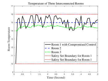
Figure 2: The temperature of each room $1$, $2$ and $3$ over $50$ time steps. Room $1$ is compromised and rooms $2,3$ are protected from failure and attack. The temperature of room $1$ is depicted using solid black line. The temperature of room $2$ is shown in blue dash line. The temperature of room $3$ is shown in red dash-dotted line.

VII Conclusion

In this paper, we studied the problem of safety-critical control synthesis of CPS with multiple interconnected sub-systems. We considered that a set of sub-systems are vulnerable in the sense that their controllers may incur random failures or malicious attacks. For the vulnerable sub-systems we introduced resilient-safety indices (RSIs) bounding the worst-case impacts of vulnerable systems towards the specified safety constraints. The sign of RSI indicates the contribution of vulnerable sub-system in either satisfying or violating the corresponding safety constraint whereas the magnitude quantifies such contribution. We provided a sufficient condition for the control policies in the non-vulnerable sub-systems so that the safety constraints are satisfied in the presence of failure or attack in the vulnerable sub-systems. We formulated sum-of-squares optimization programs to compute the RSIs and safety-ensuring control policies. Control policy in each sub-system can be computed independently using our proposed algorithm. We presented two special cases for which the RSIs can be found more efficiently. We demonstrated the usefulness of our proposed approach using an example on temperature regulation of interconnected rooms.

References

• [1] A. D. Ames, X. Xu, J. W. Grizzle, and P. Tabuada, “Control barrier function based quadratic programs for safety critical systems,” IEEE Transactions on Automatic Control, vol. 62, no. 8, pp. 3861–3876, 2016.
• [2] M. H. Cohen and C. Belta, “Approximate optimal control for safety-critical systems with control barrier functions,” in 59th IEEE Conference on Decision and Control (CDC).   IEEE, 2020, pp. 2062–2067.
• [3] C. Fan, K. Miller, and S. Mitra, “Fast and guaranteed safe controller synthesis for nonlinear vehicle models,” in International Conference on Computer Aided Verification.   Springer, 2020, pp. 629–652.
• [4] J. E. Sullivan and D. Kamensky, “How cyber-attacks in Ukraine show the vulnerability of the US power grid,” The Electricity Journal, vol. 30, no. 3, pp. 30–35, 2017.
• [5] A. Greenberg, “Hackers remotely kill a Jeep on the highway–with me in it,” 2015. [Online]. Available: https://www.wired.com/2015/07/hackers-remotely-kill-jeep-highway/
• [6] X. Xu, “Constrained control of input–output linearizable systems using control sharing barrier functions,” Automatica, vol. 87, pp. 195–201, 2018.
• [7] S. Prajna, A. Jadbabaie, and G. J. Pappas, “A framework for worst-case and stochastic safety verification using barrier certificates,” IEEE Transactions on Automatic Control, vol. 52, no. 8, pp. 1415–1428, 2007.
• [8] F. Björck, M. Henkel, J. Stirna, and J. Zdravkovic, “Cyber resilience–fundamentals for a definition,” in New Contributions in Information Systems and Technologies.   Springer, 2015, pp. 311–316.
• [9] Q. Zhu and T. Başar, “Game-theoretic methods for robustness, security, and resilience of cyberphysical control systems: games-in-games principle for optimal cross-layer resilient control systems,” IEEE Control Systems Magazine, vol. 35, no. 1, pp. 46–65, 2015.
• [10] R. Ivanov, M. Pajic, and I. Lee, “Attack-resilient sensor fusion for safety-critical cyber-physical systems,” ACM Transactions on Embedded Computing Systems (TECS), vol. 15, no. 1, pp. 1–24, 2016.
• [11] H. Fawzi, P. Tabuada, and S. Diggavi, “Secure estimation and control for cyber-physical systems under adversarial attacks,” IEEE Transactions on Automatic control, vol. 59, no. 6, pp. 1454–1467, 2014.
• [12] S. M. Rinaldi, J. P. Peerenboom, and T. K. Kelly, “Identifying, understanding, and analyzing critical infrastructure interdependencies,” IEEE Control Systems Magazine, vol. 21, no. 6, pp. 11–25, 2001.
• [13] Y. Zhang and O. Yağan, “Robustness of interdependent cyber-physical systems against cascading failures,” IEEE Transactions on Automatic Control, vol. 65, no. 2, pp. 711–726, 2019.
• [14] C. E. R. Commision, “Report on the grid disturbances on 30th July and 31st July 2012,” 2012. [Online]. Available: http://www.cercind.gov.in/2012/ orders/Final_Report_Grid_Disturbance.pdf.
• [15] A. Nejati, S. Soudjani, and M. Zamani, “Compositional construction of control barrier certificates for large-scale stochastic switched systems,” IEEE Control Systems Letters, vol. 4, no. 4, pp. 845–850, 2020.
• [16] C. Sloth, G. J. Pappas, and R. Wisniewski, “Compositional safety analysis using barrier certificates,” in Proceedings of the 15th ACM International Conference on Hybrid Systems: Computation and Control, 2012, pp. 15–24.
• [17] Z. Lyu, X. Xu, and Y. Hong, “Small-gain theorem for safety verification of interconnected systems,” Automatica, vol. 139, p. 110178, 2022.
• [18] S. Coogan and M. Arcak, “A dissipativity approach to safety verification for interconnected systems,” IEEE Transactions on Automatic Control, vol. 60, no. 6, pp. 1722–1727, 2014.
• [19] H. Yang, B. Jiang, M. Staroswiecki, and Y. Zhang, “Fault recoverability and fault tolerant control for a class of interconnected nonlinear systems,” Automatica, vol. 54, pp. 49–55, 2015.
• [20] H. Yang, C. Zhang, Z. An, and B. Jiang, “Exponential small-gain theorem and fault tolerant safe control of interconnected nonlinear systems,” Automatica, vol. 115, p. 108866, 2020.
• [21] H. Alemzadeh, D. Chen, X. Li, T. Kesavadas, Z. T. Kalbarczyk, and R. K. Iyer, “Targeted attacks on teleoperated surgical robots: Dynamic model-based detection and mitigation,” in 46th Annual IEEE/IFIP International Conference on Dependable Systems and Networks (DSN).   IEEE, 2016, pp. 395–406.
• [22] K. Koscher, S. Savage, F. Roesner, S. Patel, T. Kohno, A. Czeskis, D. McCoy, B. Kantor, D. Anderson, H. Shacham, and S. Savage, “Experimental security analysis of a modern automobile,” in IEEE Symposium on Security and Privacy.   IEEE, 2010, pp. 447–462.
• [23] E. M. Clarke, “Model checking,” in International Conference on Foundations of Software Technology and Theoretical Computer Science.   Springer, 1997, pp. 54–56.
• [24] Z. Manna and A. Pnueli, Temporal Verification of Reactive Systems: Safety.   Springer Science & Business Media, 2012.
• [25] I. M. Mitchell, A. M. Bayen, and C. J. Tomlin, “A time-dependent Hamilton-Jacobi formulation of reachable sets for continuous dynamic games,” IEEE Transactions on Automatic Control, vol. 50, no. 7, pp. 947–957, 2005.
• [26] M. Pajic, J. Weimer, N. Bezzo, P. Tabuada, O. Sokolsky, I. Lee, and G. J. Pappas, “Robustness of attack-resilient state estimators,” in ACM/IEEE International Conference on Cyber-Physical Systems (ICCPS).   ACM/IEEE, 2014, pp. 163–174.
• [27] A. A. Cárdenas, S. Amin, and S. Sastry, “Research challenges for the security of control systems.” in Proceedings of the 3rd Conference on Hot Topics in Security, vol. 5.   USENIX Association, 2008, p. 15.
• [28] M. Castro and B. Liskov, “Practical Byzantine fault tolerance and proactive recovery,” ACM Transactions on Computer Systems (TOCS), vol. 20, no. 4, pp. 398–461, 2002.
• [29] P. E. Veríssimo, N. F. Neves, and M. P. Correia, “Intrusion-tolerant architectures: Concepts and design,” in Architecting Dependable Systems.   Springer, 2003, pp. 3–36.
• [30] J. S. Mertoguno, R. M. Craven, M. S. Mickelson, and D. P. Koller, “A physics-based strategy for cyber resilience of CPS,” in Autonomous Systems: Sensors, Processing, and Security for Vehicles and Infrastructure 2019, vol. 11009.   International Society for Optics and Photonics, 2019, p. 110090E.
• [31] F. Abdi, C.-Y. Chen, M. Hasan, S. Liu, S. Mohan, and M. Caccamo, “Guaranteed physical security with restart-based design for cyber-physical systems,” in 2018 ACM/IEEE 9th International Conference on Cyber-Physical Systems (ICCPS).   ACM/IEEE, 2018, pp. 10–21.
• [32] L. Niu, D. Sahabandu, A. Clark, and P. Radha, “Verifying safety for resilient cyber-physical systems via reactive software restart,” in (accepted) 2022 ACM/IEEE 13th International Conference on Cyber-Physical Systems (ICCPS).   ACM/IEEE, 2022.
• [33] A. J. Gallo, A. Barboni, and T. Parisini, “On detectability of cyber-attacks for large-scale interconnected systems,” IFAC-PapersOnLine, vol. 53, no. 2, pp. 3521–3526, 2020.
• [34] V. Powers, “Positive polynomials and sums of squares: Theory and practice,” Real Algebraic Geometry, vol. 1, pp. 78–149, 2011.
• [35] S. Coogan and M. Arcak, “Finite abstraction of mixed monotone systems with discrete and continuous inputs,” Nonlinear Analysis: Hybrid Systems, vol. 23, pp. 254–271, 2017.
• [36] P.-J. Meyer, A. Girard, and E. Witrant, “Compositional abstraction and safety synthesis using overlapping symbolic models,” IEEE Transactions on Automatic Control, vol. 63, no. 6, pp. 1835–1841, 2017.