Learning Disentangled Representations of Negation and Uncertainty

Abstract

Negation and uncertainty modeling are long-standing tasks in natural language processing. Linguistic theory postulates that expressions of negation and uncertainty are semantically independent from each other and the content they modify. However, previous works on representation learning do not explicitly model this independence. We therefore attempt to disentangle the representations of negation, uncertainty, and content using a Variational Autoencoder. We find that simply supervising the latent representations results in good disentanglement, but auxiliary objectives based on adversarial learning and mutual information minimization can provide additional disentanglement gains.

1 Introduction

In formal semantics, negation and uncertainty are operators whose semantic functions are independent of the propositional content they modify Cann (1993a, b). That is, it is possible to form fluent statements by varying only one of these aspects while leaving the others the same. Negation, uncertainty, and content can thus be viewed as disentangled generative factors of knowledge and belief statements (see Figure 1).

Disentangled representation learning (DRL) of factors of variation can improve the robustness of representations and their applicability across tasks Bengio et al. (2013). Specifically, negation and uncertainty are important for downstream NLP tasks such as sentiment analysis Benamara et al. (2012); Wiegand et al. (2010), question answering Yatskar (2019); Yang et al. (2016), and information extraction Stenetorp et al. (2012). Disentangling negation and uncertainty can therefore provide robust representations for these tasks, and disentangling them from content can assist tasks that rely on core content preservation such as controlled generation Logeswaran et al. (2018) and abstractive summarization Maynez et al. (2020).

Figure 1: Example indicating the distinction between uncertainty, negation and content. The content “Trees have leaves” is modified by the negation (bold) and uncertainty (underlined) factors.

Still, no previous work has tested whether negation, uncertainty, and content can be disentangled, as linguistic theory suggests, although previous works have disentangled attributes such as syntax, semantics, and style Balasubramanian et al. (2021); John et al. (2019); Cheng et al. (2020b); Bao et al. (2019); Hu et al. (2017); Colombo et al. (2021). To fill this gap, we aim to answer the following research questions:

RQ1: Is it possible to estimate a model of statements that upholds the proposed statistical independence between negation, uncertainty, and content?

RQ2: A number of existing disentanglement objectives have been explored for text, all giving promising results. How do these objectives compare for enforcing disentanglement on this task?

1.1 Contributions

In addressing these research questions, we make the following contributions:

1. Generative Model: We propose a generative model of statements in which negation, uncertainty, and content are independent latent variables. Following previous works, we estimate this model using a Variational Autoencoder (VAE) Kingma and Welling (2014); Bowman et al. (2016) and compare existing auxiliary objectives for enforcing disentanglement via a suite of evaluation metrics.

2. Simple Latent Representations: We note that negation and uncertainty have a binary function (positive or negative, certain or uncertain). We therefore attempt to learn corresponding 1-dimensional latent representations for these variables, with a clear separation between each value.

3. Data Augmentation: Datasets containing negation and uncertainty annotations are relatively small Farkas et al. (2010); Vincze et al. (2008); Jiménez-Zafra et al. (2018), resulting in poor sentence reconstructions according to our preliminary experiments. To address this, we generate weak labels for a large number of Amazon and Yelp reviews using a simple naïve Bayes classifier with bag-of-words features trained on a smaller dataset of English reviews annotated for negation and uncertainty Konstantinova et al. (2012) and use this to estimate our model. Details are given in Section 4.1.1.

We note that, in contrast to other works on negation and uncertainty modeling, which focus on token-level tasks of negation and uncertainty cue and scope detection, this work aims to learn statement-level representations of our target factors, in line with previous work on text DRL.

2 Background

We here provide relevant background on negation and uncertainty processing, disentangled representation learning in NLP, as well as discussion of how this study fits in with previous work.

2.1 Negation and Uncertainty in NLP

Negation and uncertainty help determine the asserted veracity of statements and events in text Saurí and Pustejovsky (2009); Thompson et al. (2017); Kilicoglu et al. (2017), which is crucial for downstream NLP tasks that deal with knowledge and belief. For example, negation detection has been shown to provide strong cues for sentiment analysis Barnes et al. (2021); Ribeiro et al. (2020) and uncertainty detection assists with fake news detection Choy and Chong (2018). Previous works on negation and uncertainty processing focus on the classification tasks of cue identification and scope detection Farkas et al. (2010) using sequence models such as conditional random fields (CRFs) Jiménez-Zafra et al. (2020); Li and Lu (2018), convolutional and recurrent neural networks (CNNs and RNNs) Qian et al. (2016); Adel and Schütze (2017); Ren et al. (2018), LSTMs Fancellu et al. (2016); Lazib et al. (2019), and, most recently, transformer architectures Khandelwal and Sawant (2020); Lin et al. (2020); Zhao and Bethard (2020). While these works focus mostly on learning local representations of negation and uncertainty within a sentence, we attempt to learn global representations that encode high-level information regarding the negation and uncertainty status of statements.

2.2 Disentangled Representation Learning

There is currently no agreed-upon definition of disentanglement. Early works on DRL attempt to learn a single vector space in which each dimension is independent of the others and represents one ground-truth generative factor of the object being modeled Higgins et al. (2016). Higgins et al. (2018) give a group-theoretic definition, according to which generative factors are mapped to independent vector spaces. This definition relaxes the earlier assumption that representations ought to be single-dimensional and formalizes the notion of disentanglement according to the notion of invariance. Shu et al. (2019) decompose the invariance requirement into consistency and restrictiveness, which describe specific ideal properties of the invariances between representations and generative factors. In addition to independence and invariance, interpretability is an important criterion for disentanglement. Higgins et al. (2016) point out that while methods such as PCA are able to learn independent latent representations, because these are not representative of interpretable factors of variation, they are not disentangled. We therefore want our learned representations to be predictive of meaningful factors of variation. We adopt the term informativeness from Eastwood and Williams (2018) to signify this desideratum.

Previous works on DRL for text all use some form of supervision to enforce informativeness of the latent representations. Hu et al. (2017), John et al. (2019), Cheng et al. (2020b), and Bao et al. (2019) all use gold-standard labels of the generative factors, while other works employ similarity metrics Chen and Batmanghelich (2020); Balasubramanian et al. (2021). In contrast, our approach uses weak labels for negation and uncertainty generated using a classifier trained on a small set of gold-standard data.

These previous works on text DRL all use a similar architecture: a sequence VAE Kingma and Welling (2014); Bowman et al. (2016) maps inputs to $L$ distinct vector spaces, each of which are constrained to represent a different target generative factor via a supervision signal. We also employ this overall architecture for model estimation and use it as a basis for experimenting with existing disentanglement objectives based on adversarial learning John et al. (2019); Bao et al. (2019) and mutual information minimization Cheng et al. (2020b), described in Section 3.4. However, unlike these previous works, which learn high-dimensional representations of all the latent factors, we aim to learn 1-dimensional representations of the negation and uncertainty variables in accordance with their binary function.

Figure 2: Graph of the generative model. $c$ is content, $n$ is negation status, and $u$ is uncertainty.

3 Proposed Approach

We describe our overall model in Section 3.1. Section 3.2 enumerates three specific desiderata for disentangled representations, and sections 3.3 and 3.4 describe how we aim to satisfy these desiderata.

3.1 Generative Model

We propose a generative model of statements according to which negation, uncertainty, and content are independent latent variables. A diagram of our proposed model is given in Figure 2. Model details are given in Appendix A.

We use a sequence VAE to estimate this model Kingma and Welling (2014); Bowman et al. (2016). Unlike a standard autoencoder, the VAE imposes a prior distribution on the latent representation space $Z$ (usually a standard Gaussian) and replaces the deterministic encoder with a learned approximation of the posterior $q_{\phi}(z|x)$ parameterized by a neural network. In addition to minimizing the loss between the input and reconstruction, as in a standard AE, the VAE uses an additional KL divergence term to keep the approximate posterior close to the prior distribution.

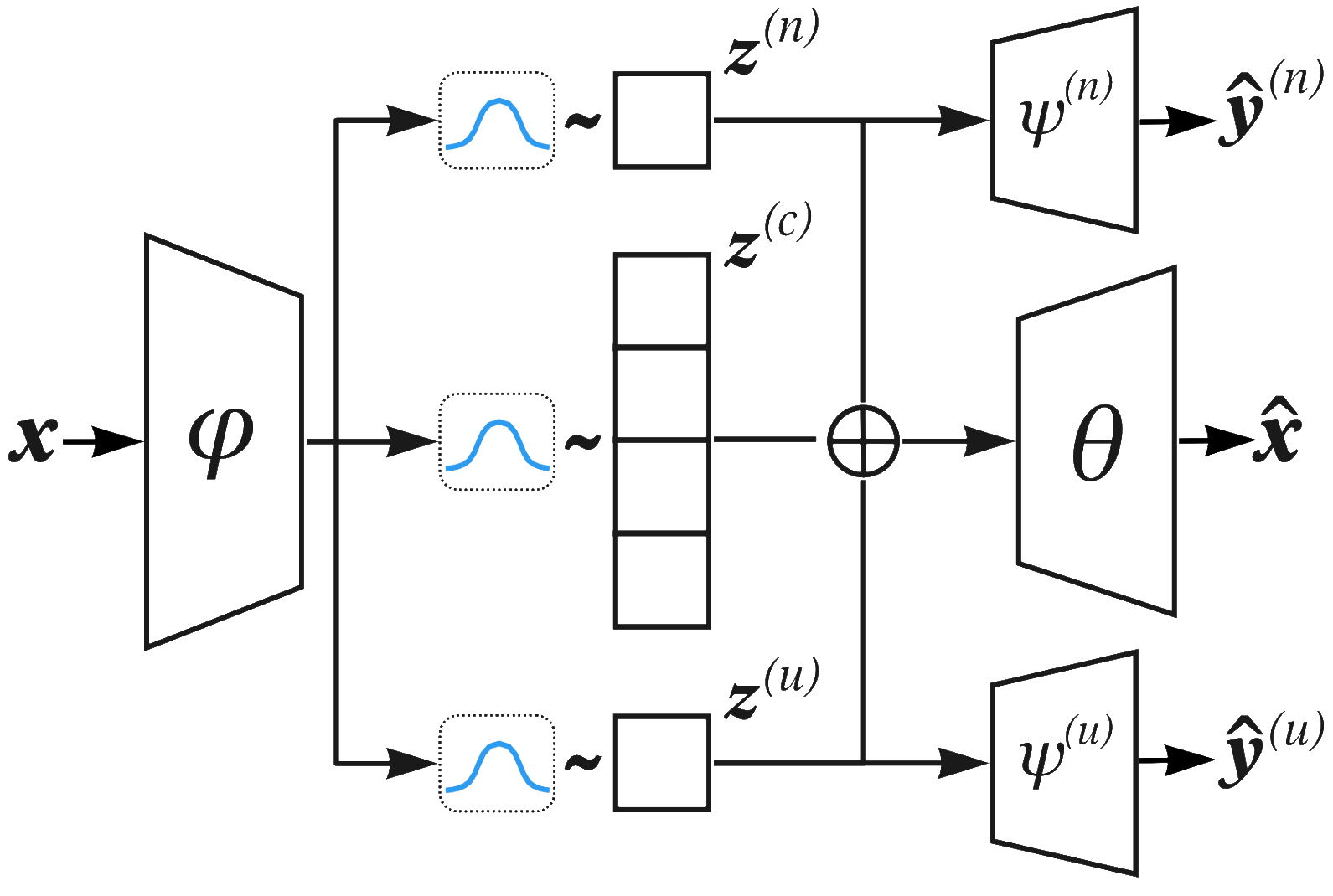
Figure 3: The proposed architecture corresponding to the $\mathcal{L}_{ELBO}+\mathcal{L}_{INF}$ objective (see Section 3.4). A BiLSTM encoder parameterized by $\phi$ maps each input example $x$ to three distinct distributions from which the latent representations $z^{(\ell)}$ are sampled. The negation $z^{(n)}$ and uncertainty $z^{(u)}$ latent spaces are then passed to linear classifiers, parameterized by $\psi^{(\ell)}$, which attempt to predict the ground truth factor. Finally, the latent values initialize an LSTM decoder, parameterized by $\theta$, which attempts to reconstruct the input.

In our implementation, three linear layers map the final hidden state of a BiLSTM encoder to three sets of Gaussian distribution parameters ($\mu$, $\sigma$), which parameterize the negation, uncertainty, and content latent distributions $\ell\in\{n,u,c\}$, respectively. Because we map each input to three distinct latent spaces, we include three KL divergence terms in the Evidence Lower BOund (ELBO) training objective, given in Equation 1.

$$\mathcal{L}_{\mathrm{ELBO}}(\phi,\theta)=-\mathbb{E}_{q_{\phi}(z|x)}\Big{[}\text{log}~{}p_{\theta}(x|z)\Big{]}$$

$$+\sum_{\ell\in\{n,u,c\}}\beta_{\ell}~{}\text{KL}\Big{[}q^{(\ell)}_{\phi}(z^{(\ell)}|x)~{}||~{}p(z^{(\ell)})\Big{]}$$ (1)

where $\phi$ denotes the encoder’s parameters, $\theta$ the decoder’s parameters, $p(z^{(\ell)})$ is a standard Gaussian prior, and the $\beta_{\ell}$ hyper-parameters weight the KL divergence term for each latent space $\ell\in L$. The latent representations $z^{\ell}$ are sampled from normal distributions defined by these parameters using the reparameterization trick Kingma and Welling (2014), i.e., $z^{(\ell)}=\mu^{(\ell)}\odot\sigma^{(\ell)}+\epsilon\sim\mathcal{N}({\bf 0},{\bf I})$. The latent representations are then concatenated $z=[z^{(n)};z^{(u)};z^{(c)}]$ and used to initialize an LSTM decoder, which aims to reconstruct the input. A visualization of our architecture is given in Figure 3 and implementation details are given in Appendix E.

We use 1-dimensional negation and uncertainty spaces and a 62-dimensional content space for a total latent size of 64. Notably, we do not supervise the content space, unlike previous works John et al. (2019); Cheng et al. (2020b), which supervise it by predicting the bag of words of the input. Such a supervision technique would hinder disentanglement by encouraging the content space to be predictive of the negation and uncertainty cues. Therefore, in our model we define three latent spaces $\ell\in\{n,u,c\}$ but use signals from only 2 target generative factors $k\in\{n,u\}$.

3.2 Desiderata for Disentanglement

We aim to satisfy the following desiderata of disentangled representations put forth by previous works.

1. Informativeness: the representations should be predictive of the ground-truth generative factors Higgins et al. (2016); Eastwood and Williams (2018);

2. Independence: the representations for each generative factor in question should lie in independent vector spaces Higgins et al. (2018);

3. Invariance: the mapping from the data to the representations should be invariant to changes in other generative factors Higgins et al. (2018); Shu et al. (2019);

The following sections detail how our model enforces these desiderata.

3.3 Informativeness

Following Eastwood and Williams (2018), we measure the informativeness of a representation by its ability to predict the corresponding generative factor. Similar to previous works on DRL for text John et al. (2019); Cheng et al. (2020b), we train supervised linear classifiers on each latent space and back-propagate the prediction error. Thus, in addition to the ELBO objective in Equation 1, we define informativeness objectives for negation and uncertainty.

$$\mathcal{L}_{\mathrm{INF}}(\psi^{(k)})=\mathrm{BCE}\Big{(}\hat{y}^{(k)},y^{(k)}\Big{)},~{}~{}k\in\{n,u\}$$ (2)

where $y^{(k)}$ is the true label for factor $k$, $\hat{y}^{(k)}$ is the classifier’s prediction, $\psi^{(k)}$ are the parameters of this classifier, and BCE is the binary cross-entropy loss.

3.4 Independence and Invariance

We compare 3 objectives for enforcing these desiderata:

1. Informativeness (INF): This is based on the hypothesis that if negation, uncertainty, and content are independent generative factors, the informativeness objective described in Section 3.3 will be sufficient to drive independence and invariance. This approach was found to yield good results on disentangling style from content by Balasubramanian et al. (2021).

2. Adversarial (ADV): The latent representations should be predictive of their target generative factor only. Therefore, inspired by John et al. (2019), we train additional adversarial classifiers on each latent space that try to predict the values of the non-target generative factors, while the model attempts to structure the latent spaces such that the predictive distribution of these classifiers is a non-predictive as possible.

3. Mutual-information minimization (MIN): A natural measure of independence between two variables is mutual information (MI). Therefore, this objective minimizes an upper-bound estimate of the MI between each pair of latent spaces, following Cheng et al. (2020a, b); Colombo et al. (2021).

Details on the ADV and MIN objectives are given below.

Adversarial Objective.

The adversarial objective (ADV) consists of two parts: 1) adversarial classifiers which attempt to predict the value of all non-target factors from each latent space; 2) a loss that aims to maximize the entropy of the predicted distribution of the adversarial classifiers.

For a given latent space $\ell$, a set of linear classifiers predict the value of each non-target factor $k\neq\ell$, respectively, and we compute the binary cross-entropy loss for each.

$$\mathcal{L}_{\mathrm{CLS}}(\xi^{(\ell,k)})=\mathrm{BCE}\left(\hat{y}^{(\ell,k)},y^{(k)}\right)$$ (3)

Where $\xi^{(\ell,k)}$ are the parameters of the adversarial classifier predicting factor $k$ from latent space $\ell$, and $\hat{y}^{(\ell,k)}$ is the corresponding prediction.

For example, we introduce two such classifiers for the content space $\ell=c$, one to predict negation and one to predict uncertainty, $k\in\{n,u\}$. Importantly, the prediction errors of these classifiers are not back-propagated to the rest of the VAE. We impose an additional objective for each adversarial classifier, which aims to make it’s predicted distribution as close to uniform as possible. We do this by maximizing the entropy of the predicted distribution (Equation 4) and back-propagating the error, following John et al. (2019) and Fu et al. (2018).

$$\mathcal{L}_{\mathrm{ENT}}(\xi^{(\ell,k)})=H[\hat{y}^{(\ell,k)}]$$ (4)

As the objective is to maximize this quantity, the total adversarial objective is

$$\mathcal{L}_{\mathrm{ADV}}=\sum_{\ell}\sum_{k}\mathcal{L}_{\mathrm{CLS}}(\xi^{(\ell,k)})-\mathcal{L}_{\mathrm{ENT}}(\xi^{(\ell,k)})$$ (5)

The ADV objective aims to make the latent representations as uninformative as possible for non-target factors. Together with the informativeness objective, it pushes the representations to specialize in their target generative factors.

MI Minimization Objective.

The MI minimization (MIN) objective focuses on making the distributions of each latent space as dissimilar as possible. We minimize the MI between each pair of latent spaces according to Equation 6.

$$\mathcal{L}_{\mathrm{MIN}}=\hat{I}_{\mathrm{CLUB}}(\ell_{i};\ell_{j}),~{}~{}i\neq j$$ (6)

where $\hat{I}_{\mathrm{CLUB}}(\ell_{i};\ell_{j})$ is the Contrastive Learning Upper-Bound (CLUB) estimate of the MI Cheng et al. (2020a). Specifically, we introduce a separate neural network to approximate the conditional variational distribution $p_{\sigma}(\ell_{i}|\ell_{j})$, which is used to estimate an upper bound on the MI using samples from the latent spaces.

The full model objective along with relevant hyperparameters weights $\bm{\lambda}$ is given in Equation 7. Our hyperparameter settings and further implementation details are given in Appendix E.

$$\mathcal{L}= \mathcal{L}_{\mathrm{ELBO}}+\lambda_{\mathrm{INF}}\mathcal{L}_{\mathrm{INF}}+$$

$$\lambda_{\mathrm{ADV}}\mathcal{L}_{\mathrm{ADV}}+\lambda_{\mathrm{MIN}}\mathcal{L}_{\mathrm{MIN}}$$ (7)

In the sections that follow, we experiment with different subsets of the terms in the full objective and their effects on disentanglement. We train a model using only the ELBO objective as our disentanglement baseline.

4 Experiments

We describe our datasets, preprocessing, and data augmentation methods in Section 4.1. Section 4.2 describes our evaluation metrics and how these target the desiderata for disentanglement given in Section 3.2.

4.1 Datasets

We use the SFU Review Corpus Konstantinova et al. (2012) as our primary dataset. This corpus contains 17,000 sentences from reviews of various products in English, originally intended for sentiment analysis, annotated with negation and uncertainty cues and their scopes. Many of the SFU sentences are quite long ($>30$ tokens), and preliminary experiments revealed that this results in poor reconstructions. We therefore took advantage of SFU’s annotated statement conjunction tokens to split the multi-statement sentences into single-statement ones in order to reduce the complexity and increase the number of examples. Also to reduce complexity, we remove sentences $>15$ tokens following previous work Hu et al. (2017), resulting in 14,000 sentences.

We convert all cue-scope annotations to statement-level annotations. Multi-level uncertainty annotations have been shown to be rather inconsistent and noisy, achieving low inter-annotator agreement compared to binary ones Rubin (2007). We therefore binarize the certainty labels following Zerva (2019).

4.1.1 Data Augmentation

Despite the efforts above, we found the SFU corpus alone was insufficient for obtaining fluent reconstructions. We therefore generated weak negation and uncertainty labels for a large amount of additional Amazon and Yelp review data using two naïve Bayes classifiers with bag-of-words (BOW) features. These classifiers were trained on the SFU training split to predict sentence level negation and uncertainty, respectively. The Amazon and Yelp datasets fit the SFU data distribution well, being also comprised of user reviews, and have been used in previous works on text DRL with good results John et al. (2019); Cheng et al. (2020b). Statistics for the combined SFU+Amazon dataset are summarized in Appendix C. In Appendix D, we provide a complementary evaluation on a combined SFU+Yelp dataset.

4.2 Evaluation

Evaluating disentanglement of the learned representations requires complementary metrics of the desiderata given in Section 3.2: informativeness, independence, and invariance.

For measuring informativeness, we report the precision, recall, and F1 score of a logistic regression model trained to predict each of the ground-truth labels from each latent space, following Eastwood and Williams (2018). We also report the MI between each latent distribution and factor, as this gives additional insight into informativeness.

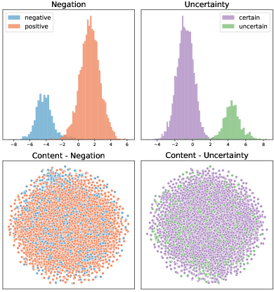
Figure 4: Histogram and t-SNE Van der Maaten and Hinton (2008) visualizations of the modality, negation, and content spaces learned by the INF+ADV+MIN model.

For measuring independence, we use the Mutual Information Gap (MIG) Chen et al. (2018). The MIG lies in $[0,1]$, with higher values indicating a greater degree of disentanglement. Details of the MIG computation are give in Section E.1.

We evaluate invariance by computing the Pearson’s correlation coefficient between each pair of latent variables using samples from the predicted latent distributions.

		$\mathcal{L}_{\mathrm{ELBO}}$				+$\mathcal{L}_{\mathrm{INF}}$				+$\mathcal{L}_{\mathrm{INF}}$+$\mathcal{L}_{\mathrm{ADV}}$+$\mathcal{L}_{\mathrm{MIN}}$
Latent	Factor	MI	P	R	F1	MI	P	R	F1	MI	P	R	F1
$n$	$n$	0.018	0.561	0.615	0.530	0.434	0.951	0.972	0.961	0.444	0.959	0.975	0.967
	$u$	0.016	0.558	0.590	0.533	0.013	0.551	0.584	0.544	0.007	0.543	0.569	0.537
$u$	$n$	0.011	0.559	0.606	0.540	0.013	0.555	0.579	0.550	0.007	0.548	0.560	0.548
	$u$	0.022	0.570	0.604	0.562	0.375	0.936	0.972	0.952	0.391	0.970	0.981	0.975
$c$	$n$	0.297	0.683	0.760	0.695	0.222	0.675	0.753	0.684	0.147	0.576	0.617	0.557
	$u$	0.207	0.653	0.756	0.665	0.198	0.643	0.746	0.649	0.136	0.574	0.637	0.551

Table 1: Mutual Information estimate between each latent and factor. Precision, recall, and F1 of the latent space classifiers for each factor. $n$: negation. $u$: uncertainty. $c$: content. Shown are the mean values computed from 30 resamples of the latent distributions for each example on the SFU+Amazon test set. Because their results are similar to $\mathcal{L}_{\mathrm{ELBO}}$+$\mathcal{L}_{\mathrm{INF}}$+$\mathcal{L}_{\mathrm{ADV}}$+$\mathcal{L}_{\mathrm{MIN}}$, the $\mathcal{L}_{\mathrm{ELBO}}$+{$\mathcal{L}_{\mathrm{ADV}}$,$\mathcal{L}_{\mathrm{MIN}}$} are not included to save space. We provide a more extensive set of results covering all models in Table 10.

It also important to evaluate the ability of the models to reconstruct the input. Specifically, we target reconstruction faithfulness (i.e., how well the input and reconstruction match) and fluency. We evaluate faithfulness in terms of the ability of the model to preserve the negation, uncertainty, and content of the input. Negation and uncertainty preservation are measured by re-encoding the reconstructions, predicting the negation and uncertainty statuses from the re-encoded latent values, and computing precision, recall, and F1 score against the ground-truth labels. Following previous work, we approximate a measure of content preservation in the absence of any explicit content annotations by computing the BLEU score between the input and the reconstruction (self-BLEU) Bao et al. (2019); Cheng et al. (2020b); Balasubramanian et al. (2021). We evaluate fluency of the reconstruction by computing the perplexities (PPL) under GPT-2, a strong, general-domain language model Radford et al. (2019).

Finally, we evaluate the models’ ability to flip the negation or uncertainty status of the input. For each test example, we override the value of the latent factor we want to change to represent the opposite of its ground-truth label. The ability of the model to control negation and uncertainty is measured by re-encoding the reconstructions obtained from the overridden latents, predicting from the re-encoded latent values, and computing accuracy against the opposite of the ground-truth labels.

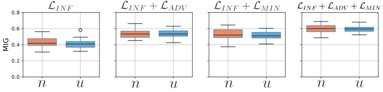
Figure 5: Box plots of the Mutual Information Gap (MIG) for each disentanglement objective for the negation and uncertainty factors computed on the test set. The MIG values for the baseline $\mathcal{L}_{\mathrm{ELBO}}$ objective were too small to include in this figure, at $\approx 0.014$ for both negation and uncertainty.

5 Results

In the following, Section 5.1 reports the disentanglement results and Section 5.2 reports the faithfulness and fluency results. Section 5.3 discusses how these results address the two research questions proposed in Section 1.

5.1 Disentanglement

The informativeness of each latent space with respect to each target factor is shown in Table 1 given as predictive performance and MI.

The baseline ELBO objective alone fails to disentangle. It puts almost all representation power in the content space, which is nevertheless still uninformative of the negation and uncertainty factors, with low MIs and F1s. The model using the INF auxiliary objective does, however, manage to achieve good disentanglement: the negation and uncertainty spaces are highly informative of their target factors and uninformative of the non-target factors. However, the content space is still slightly predictive of negation and uncertainty, with F1s of 0.684 and 0.649, respectively. This improves with the ADV and MIN objectives, where the content space shows near-random prediction performance of negation and uncertainty, with slightly improved prediction performance of the negation and uncertainty spaces for their target factors. These results are corroborated by the visualizations in Figure 4, which show clear separation by classes in the negation and uncertainty latent distributions but no distinction between classes in the content space. Additionally, we note the good predictive performance of the negation and uncertainty latents, despite their simple, 1-dimensional encoding.

+$\mathcal{L}_{\mathrm{INF}}$+$\mathcal{L}_{\mathrm{ADV}}$ $\mathcal{L}_{\mathrm{ELBO}}$ +$\mathcal{L}_{\mathrm{INF}}$ +$\mathcal{L}_{\mathrm{MIN}}$ $u$ $c$ $u$ $c$ $u$ $c$ $n$ 0.706 0.008 0.200 0.002 0.159 0.001 ($\pm 0.053$) ($\pm 0.098$) ($\pm 0.043$) $u$ - 0.001 - 0.001 - 0.005 ($\pm 0.058$) ($\pm 0.097$) ($\pm 0.037$)

Table 2: Pearson’s correlation coefficients between each pair of latent representations across models. As the content space is 62-dimensional, we compute the correlation coefficient between each dimension and report the mean with the standard deviation in parentheses below.

Box plots of the MIG values for the negation and uncertainty factors are given in Figure 5. Again we see that the INF objective alone results in decent disentanglement, with median MIG values $\approx 0.4$. The ADV and MI objectives give similar increases in MIG, up to $\approx 0.55$ for both negation and uncertainty, and their combination, ADV+MIN, improves MIG further, up to $\approx 0.6$, suggesting that these objectives are complementary.

We demonstrate the invariance of our models’ negation and uncertainty representations in Table 2. While the ELBO objective alone results in highly covariant negation and uncertainty latent distributions (0.706), this drops significantly under INF (0.200) with additional reduction contributed by the ADV and MIN objectives (0.159).

5.2 Evaluation of Reconstructions

5.2.1 Faithfulness and Fluency

Table 3 reports the self-BLEU and perplexity for each disentanglement objective. Example reconstructions are given in Table 9. These results show that the models are quite consistent regarding content reconstruction on the train set, but this consistency drops on dev and test. While the ADV and MIN objectives provide disentanglement gains over INF, the BLEU scores betray a possible trade off of slightly poorer content preservation, despite better perplexities.

						+$\mathcal{L}_{\mathrm{INF}}$
				+$\mathcal{L}_{\mathrm{INF}}$	+$\mathcal{L}_{\mathrm{INF}}$	+$\mathcal{L}_{\mathrm{ADV}}$
		$\mathcal{L}_{\mathrm{ELBO}}$	+$\mathcal{L}_{\mathrm{INF}}$	+$\mathcal{L}_{\mathrm{ADV}}$	+$\mathcal{L}_{\mathrm{MIN}}$	+$\mathcal{L}_{\mathrm{MIN}}$
BLEU	Train	0.590	0.576	0.574	0.528	0.522
	Dev	0.150	0.189	0.186	0.146	0.141
	Test	0.153	0.072	0.073	0.148	0.144
PPL	Train	123.3	174.3	173.1	124.9	127.2
	Dev	136.4	186.1	189.1	140.1	141.3
	Test	136.8	185.9	187.3	139.3	142.1

Table 3: Reconstruction self-BLEU and reconstruction perplexity (PPL) for each model on each data split. Perplexity is computed using GPT-2 Radford et al. (2019).

While self-BLEU indicates the consistency of the reconstructions with respect to content, it does not necessarily indicate consistency of the reconstructions with respect to negation and uncertainty, which often differ from their opposite value counterparts by a single token. The consistency of the INF and INF+ADV+MIN models with respect to these factors is reported in Table 4. The INF objective alone is only somewhat consistent, with re-encoded F1s of 0.830 and 0.789 for negation and uncertainty respectively. The auxiliary objectives improve these considerably, to 0.914 and 0.893, suggesting that the disentanglement gains seen in Table 1 and Figure 5 have a positive effect on the consistency of the reconstructions.

+$\mathcal{L}_{\mathrm{INF}}$+$\mathcal{L}_{\mathrm{ADV}}$ +$\mathcal{L}_{\mathrm{INF}}$ +$\mathcal{L}_{\mathrm{MIN}}$ Factor Pass P R F1 P R F1 $n$ 1 0.969 0.965 0.967 0.959 0.975 0.967 2 0.816 0.848 0.830 0.920 0.908 0.914 $u$ 1 0.959 0.961 0.960 0.970 0.981 0.975 2 0.767 0.820 0.789 0.930 0.864 0.893

Table 4: Consistency of the decoder with the ground-truth values of negation and uncertainty evaluated on the test set. Pass 1 refers to the predictions from the original inputs. Pass 2 refers to the predictions from the re-encoded reconstructions. Pass 1 can be considered an upper bound on the performance of pass 2.

5.2.2 Controlled Generation

Table 5 shows the accuracies of each model on the controlled generation task, split by transfer direction. We found that for both negation and uncertainty modifying the status of the input works well in only one direction: from negated to positive, uncertain to certain.

Changing a sentence from negated to positive or from uncertain to certain generally requires the removal of cue tokens (e.g., not, never, might), while the opposite directions require their addition. Via linear regressions between the content representations and number of tokens, we found that the content space is highly informative of sentence length, which effectively bars the decoder from adding the required negation or uncertainty tokens. A manual review of correctly and incorrectly modified sentences suggested that the decoder attempts to represent the negation/uncertainty status by modifying tokens in the input, rather than adding or removing them, in order to satisfy the length constraint. When removal is required, the cue token is often simply replaced by new tokens consistent with the representation. The inclusion of negation/uncertainty cue tokens, however, only seems to occur when it is possible to change an existing token to a cue token. Details of the linear regressions as well as example successful/failed transfers are given in Section C.3.

+$\mathcal{L}_{\mathrm{INF}}$ +$\mathcal{L}_{\mathrm{INF}}$ +$\mathcal{L}_{\mathrm{INF}}$ +$\mathcal{L}_{\mathrm{ADV}}$ Transfer direction +$\mathcal{L}_{\mathrm{INF}}$ +$\mathcal{L}_{\mathrm{ADV}}$ +$\mathcal{L}_{\mathrm{MIN}}$ +$\mathcal{L}_{\mathrm{MIN}}$ pos $\rightarrow$ neg 0.30 0.50 0.35 0.38 neg $\rightarrow$ pos 0.80 0.92 0.79 0.87 cer $\rightarrow$ unc 0.34 0.40 0.32 0.36 unc $\rightarrow$ cer 0.85 0.88 0.80 0.86

Table 5: Controlled generation accuracies by factor and direction of transfer.

5.3 Research Questions

RQ1: Is it possible to learn disentangled representations of negation, uncertainty, and content?
The results suggest that it is indeed possible to estimate a statistical model in which negation, uncertainty, and content are disentangled latent variables according to our three desiderata outlined in Section 3.2. Specifically, Table 1 shows high informativeness of the negation and uncertainty spaces across objectives, and the poor predictive ability of each latent space for non-target factors suggests independence. Figure 5 further suggests independence across models, with median MIG scores in the 0.4-0.6 range. Finally, the low covariances in Table 2 demonstrates the invariance of the latent representations to each other.

RQ2: How do existing disentanglement objectives compare for this task?
Notably, the INF objective alone results in good disentanglement according to our three desiderata, suggesting that supervision alone is sufficient for disentanglement. Still, the addition of the ADV and MIN objectives resulted in slightly more informative (Table 1) and independent (Table 2) representations. While the self-BLEU scores reported in Table 3 suggest that content preservation is generally maintained across auxiliary objectives, small dips are seen in those using the MIN objective. This trend also holds for perplexity, suggesting that while the MIN objective can contribute to disentanglement gains, it may result in poorer reconstructions.

6 Conclusion

Motivated by linguistic theory, we proposed a generative model of statements in which negation, uncertainty, and content are disentangled latent variables. We estimated this model using a VAE, comparing the performance of existing disentanglement objectives. Via a suite of evaluations, we showed that it is indeed possible to disentangle these factors. While objectives based on adversarial learning and MI minimization resulted in disentanglement and consistency gains, we found that a decent balance between variable disentanglement and reconstruction ability was obtained by a simple supervision of the latent representations (i.e., the INF objective). Also, our 1-dimensional negation and uncertainty representations achieved high predictive performance, despite their simplicity. Future work will explore alternative latent distributions, such as discrete distributions Jang et al. (2017); Dupont (2018), which may better represent these operators.

This work has some limitations. First, our model does not handle negation and uncertainty scope, but rather assumes that operators scope over the entire statement. Our model was estimated on relatively short, single-statement sentences to satisfy this assumption, but future work will investigate how operator disentanglement can be unified with models of operator scope in order to apply it to longer examples with multiple clauses. Second, while our models achieved high disentanglement, they fell short on the controlled generation task. We found that this was likely due to the models memorizing sentence length, constraining the reconstructions in way that is incompatible with the addition of negation and uncertainty cue tokens. (Bosc and Vincent, 2020) also noticed this tendency for sentence length memorization in VAEs and future will will explore their suggested remedies, such as encoder pretraining.

Appendix A Model Details

We here define our generative model and derive the corresponding ELBO objective for our proposed VAE with three latent variables. Let $x=[x_{1},...,x_{T}]$ be a sentence with $T$ tokens. $N$, $U$, and $C$ are the latent variables representing negation, uncertainty, and content respectively. The joint probability of specific values of these variables ($N=n$, $U=u$, $C=c$) is defined as

$$p(x,n,u,c)=p_{\theta}(x|n,u,c)p(n)p(u)p(c)$$ (8)

Furthermore, $x$ is defined auto-regressively as

$$p(x|n,u,c)=\prod_{t}p(x_{t}|x_{<t},n,u,c)$$ (9)

Our model assumes that the latent factors are independent, so the posterior is

$$p(n,u,c|x) =p(n|x)p(u|x)p(c|x)$$ (10)

$$=\prod_{\ell\in\{n,u,c\}}\frac{p(x|\ell)p(\ell)}{p(x)}$$ (11)

We approximate the posterior $p(n,u,c|x)$ with $q_{\phi}(n,u,c|x)$. Because the posterior factors, we approximate the individual posteriors $p(\cdot|x)$ with $q_{\phi}(\cdot|x)$ and derive the following ELBO objective.

ELBO $$=\mathbb{E}_{q_{\phi}(n,u,c|x)}\left[\text{log}\frac{p(x,n,u,c)}{q_{\phi}(n,u,c|x)}\right]$$ (12)

$$=\mathbb{E}_{q_{\phi}}\left[\text{log}\frac{p(x|n,u,c)p(n)p(u)p(c)}{q_{\phi}(n|x)q_{\phi}(u|x)q_{\phi}(c|x)}\right]$$ (13)

$$=\mathbb{E}_{q_{\phi}}\left[\text{log}~{}p(x|n,u,c)\right]$$ (14)

$$~{}~{}~{}~{}~{}~{}-\sum_{\ell}KL\left[q_{\phi}(\ell|x)||p(\ell)\right]$$

Appendix B Bag-of-Words Classifiers

We here provide the implementation details and evaluation of our bag-of-words (BOW) classifiers used to generate weak labels for the Amazon and Yelp data.

B.1 Implementation Details

Both classifiers are implemented as Bernoulli naïve Bayes classifiers with BOW features. We used the BernoulliNB implementation from scikit-learn with the default parameters in version 0.24.1(Pedregosa et al., 2011).

B.1.1 Feature Selection

We performed feature selection by computing the $K$ tokens from the SFU training data that had the highest ANOVA F-value against the target labels, implemented using f_classif in scikit-learn (Pedregosa et al., 2011). We tuned $K$ according to the downstream classification performance on the SFU dev set. We evaluated $K$ in the range 3-30 and found $K=20$ performed best for both models. The 20 tokens ultimately used as features by the negation and uncertainty classifiers are given in Table 6.

Negation	any, but, ca, cannot, did, do, does, dont, either, even, have, i, it, n’t, need, never, no, not, without, wo
Uncertainty	be, can, could, either, i, if, may, maybe, might, must, or, perhaps, probably, seem, seemed, seems, should, think, would, you

Table 6: The tokens used as features for the negation and uncertainty classifiers. Contractions are split in our tokenization scheme.

B.2 Evaluation

We report the precision, recall, and F1 score of both classifiers on the SFU dev and test sets in Table 7.

		P	R	F1
Negation	dev	0.942	0.877	0.901
	test	0.946	0.880	0.909
Uncertainty	dev	0.959	0.953	0.956
	test	0.948	0.961	0.954

Table 7: Precision, recall, and F1 score of the negation and uncertainty classifiers on the SFU dev and test sets.

Appendix C Additional Results on SFU+Amazon

C.1 Dataset Statistics

Split N Median % Negated % Uncertain Length Train 109,889 12 22.7% 17.9% Dev 6,631 12 19.6% 15.2% Test 6,579 12 20.4% 15.2%

Table 8: Statistics for the combined SFU and weakly labeled Amazon dataset.

C.2 Example Reconstructions

Input going home early. going home later. Recon going home movies. going home first. Input this is a second outlet there is one on the dash. this is a second blender there is one on the floor. Recon this is a second computer there is one on the seatbelt. this is a second grease there is one on the cat. Input sometime it’s just not enough volume. guess it’s just not enough power. Recon believe it works just not pleasant enough. obviously it s just not enough control. Input I would never stay there again. i would never stay them again. Recon i would never rate that again. i would not suggest that again.

Table 9: Example reconstructions decoded by the INF+ADV+MI model from the SFU+Amazon test set.

		+$\mathcal{L}_{\mathrm{INF}}$				+$\mathcal{L}_{\mathrm{INF}}$+$\mathcal{L}_{\mathrm{ADV}}$				+$\mathcal{L}_{\mathrm{INF}}$+$\mathcal{L}_{\mathrm{MIN}}$				+$\mathcal{L}_{\mathrm{INF}}$+$\mathcal{L}_{\mathrm{ADV}}$+$\mathcal{L}_{\mathrm{MIN}}$
Latent	Factor	MI	P	R	F1	MI	P	R	F1	MI	P	R	F1	MI	P	R	F1
$n$	$n$	0.434	0.951	0.972	0.961	0.431	0.952	0.970	0.961	0.443	0.962	0.977	0.969	0.444	0.959	0.975	0.967
	$u$	0.013	0.551	0.584	0.544	0.012	0.551	0.581	0.547	0.007	0.537	0.560	0.527	0.007	0.543	0.569	0.537
$u$	$n$	0.013	0.555	0.579	0.550	0.008	0.553	0.573	0.550	0.008	0.543	0.561	0.535	0.007	0.548	0.560	0.548
	$u$	0.375	0.936	0.972	0.952	0.374	0.941	0.972	0.956	0.389	0.960	0.980	0.970	0.391	0.970	0.981	0.975
$c$	$n$	0.222	0.675	0.753	0.684	0.166	0.576	0.619	0.550	0.182	0.640	0.710	0.638	0.147	0.576	0.617	0.557
	$u$	0.198	0.643	0.746	0.649	0.144	0.567	0.626	0.538	0.169	0.638	0.740	0.641	0.136	0.574	0.637	0.551

Table 10: Mutual Information estimate between each latent and factor. Precision, recall, and F1 of the latent space classifiers for each factor. Shown are the mean values computed from 30 resamples of the latents for each example on the SFU+Amazon test set.

					+$\mathcal{L}_{\mathrm{INF}}$		+$\mathcal{L}_{\mathrm{INF}}$		+$\mathcal{L}_{\mathrm{INF}}$+$\mathcal{L}_{\mathrm{ADV}}$
	$\mathcal{L}_{\mathrm{ELBO}}$		+$\mathcal{L}_{\mathrm{INF}}$		+$\mathcal{L}_{\mathrm{ADV}}$		+$\mathcal{L}_{\mathrm{MIN}}$		+$\mathcal{L}_{\mathrm{MIN}}$
	$u$	$c$	$u$	$c$	$u$	$c$	$u$	$c$	$u$	$c$
$n$	0.706	0.008	0.200	0.002	0.193	0.007	0.129	0.008	0.159	0.001
		($\pm 0.053$)		($\pm 0.098$)		($\pm 0.076$)		($\pm 0.058$)		($\pm 0.043$)
$u$	-	0.001	-	0.001	-	0.010	-	0.001	-	0.005
		($\pm 0.058$)		($\pm 0.097$)		($\pm 0.070$)		($\pm 0.060$)		($\pm 0.037$)

Table 11: Pearson’s correlation coefficients between each pair of latent representations across models on SFU+Amazon for each disentanglement objective. As the content space is 62-dimensional, we compute the correlation coefficient between each dimension and report the mean and standard deviation below in parentheses.

C.3 Controlled Generation

As discussed in Section 5.2.2, modifying the negation or certainty status of the input works well only in one direction (negated to positive, uncertain to certain). While the content space is uninformative of negation and uncertainty, we found that it is highly informative of sentence length, which hinders the decoder from adding or removing tokens to satisfy the negation/uncertainty representations. Examples of successful and failed transfers illustrating this phenomenon are given in tables 13 and 14. Table 12 reports the $R^{2}$ of linear regressions of the number of tokens in the input on samples from the negation, uncertainty, and content distributions, respectively.

Note that the transferred results have the same number of tokens as the inputs, and the decoder even repeats tokens where necessary to meet the length requirement (e.g., fit fit in the last negation example in Table 13). In general, the decoder seems to satisfy the value of the transferred factor by changing tokens in the input. This is clear in the last uncertainty example in Table 13, where the certain input is correctly changed to uncertain, but the uncertainty cue replaces the negation cue.

Latent	train	dev	test
Negation	0.048	0.057	0.063
Uncertainty	0.051	0.034	0.041
Content	0.901	0.903	0.900

Table 12: $R^{2}$ of the sentence length regression models on $z$’s sampled from INF+ADV+MIN model. $R^{2}=1$ represents perfect predictive ability.

Neg i received my lodge grill griddle and it is extremely well made. i got my kitchen steel corkscrew but it is not well made. if you do n’t have one get it now. if you must have need one used it now. but it does not fit the tmo galaxy s. but it does fit fit the net galaxy s. Unc it is light in weight and easy to clean. it is slid in sponges and seems to clean. it snaps onto the phone in two pieces. it should affect the phone in two ways. but we did n’t use it on the other one. but we would have use it on the other one.

Table 13: Successful inversions of negation and uncertainty. Inputs are in standard font and reconstructions are in italics. bold tokens indicate negation/uncertainty cues.

Neg it is light in weight and easy to clean. it is tight in light and easy to clean. the x s were fine until i washed them. the iphone s worked fine and i return them. used for months and it is still going strong. used for now and it is still going strong. Unc i received my lodge grill griddle and it is extremely well made. i received this roasting s cooking and it is still well made . glad i found these at a reasonable price. do i have these at a good price. it broke immediately when i put it on. it was immediately when i put it on.

Table 14: Failed inversions of negation and uncertainty. Inputs are in standard font and reconstructions are in italics. bold tokens indicate negation/uncertainty cues.

Appendix D Results on SFU+Yelp

Split N Median % Negated % Uncertain Length Train 390,409 9 14.5% 8.8% Dev 5,971 9 15.5% 9.1% Test 3,118 9 12.9% 10.4%

Table 15: Statistics for the combined SFU and weakly labeled Yelp dataset.

We here provide a complete evaluation of our models on a combination SFU+Yelp dataset, analogous to that performed on SFU+Amazon in the main text. Due to the shorter average length in tokens of the Yelp examples and the consequent reduction in compute power required, we were able to construct a combined dataset using the entire Yelp dataset with weak negation and uncertainty labels assigned according to the method described in § 4.1.1 of the main text. Statistics of this dataset are given in Table 15.

First, visualizations of the latent distributions in Figure 6 show 1) that the negation and uncertainty spaces are bimodal and discriminative of their corresponding factors while the content space is discriminative of neither; 2) the latent spaces are smooth and approximately normally distributed, despite two outliers.

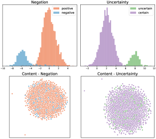
Figure 6: Histogram and t-SNE plots of the negation, uncertainty, and content spaces learned by the $\mathcal{L}_{\mathrm{ELBO}}$+$\mathcal{L}_{\mathrm{INF}}$+$\mathcal{L}_{\mathrm{ADV}}$+$\mathcal{L}_{\mathrm{MIN}}$  model on SFU+Yelp test set.

D.1 Disentanglement

The mean predictive performance of each latent space for each objective is given in Table 16, computed from 30 resamples of the latents for each test example. We also report the mean MI between each latent space and each factor over 30 resamples, as this provides additional insight into the informativeness of each space. Like the results on SFU+Amazon, these results show that the negation and uncertainty space are highly informative of their target factors and uninformative of the non-target factors. Additionally, the content space is informative of neither, showing near-random prediction performance. However, unlike the SFU+Amazon results, all objectives perform approximately equally, although the full $\mathcal{L}_{\mathrm{ELBO}}$+$\mathcal{L}_{\mathrm{INF}}$+$\mathcal{L}_{\mathrm{ADV}}$+$\mathcal{L}_{\mathrm{MIN}}$  objective does reduce the informativeness of the content space slightly compared to the other objectives.

		$\mathcal{L}_{\mathrm{ELBO}}$				+$\mathcal{L}_{\mathrm{INF}}$				+$\mathcal{L}_{\mathrm{INF}}$+$\mathcal{L}_{\mathrm{ADV}}$				+$\mathcal{L}_{\mathrm{INF}}$+$\mathcal{L}_{\mathrm{MIN}}$				+$\mathcal{L}_{\mathrm{INF}}$+$\mathcal{L}_{\mathrm{ADV}}$+$\mathcal{L}_{\mathrm{MIN}}$
Latent	Factor	MI	P	R	F1	MI	P	R	F1	MI	P	R	F1	MI	P	R	F1	MI	P	R	F1
$n$	$n$	0.020	0.560	0.628	0.555	0.308	0.916	0.954	0.934	0.307	0.913	0.954	0.932	0.308	0.911	0.953	0.931	0.307	0.920	0.954	0.936
	$u$	0.007	0.530	0.558	0.512	0.012	0.543	0.596	0.527	0.012	0.560	0.628	0.556	0.010	0.550	0.612	0.538	0.012	0.557	0.623	0.548
$u$	$n$	0.017	0.549	0.627	0.505	0.013	0.540	0.577	0.525	0.017	0.543	0.584	0.527	0.012	0.542	0.582	0.525	0.016	0.543	0.582	0.530
	$u$	0.036	0.583	0.674	0.560	0.281	0.926	0.963	0.943	0.282	0.920	0.962	0.940	0.282	0.922	0.963	0.941	0.284	0.921	0.962	0.940
$c$	$n$	0.236	0.654	0.783	0.671	0.183	0.601	0.705	0.591	0.173	0.575	0.658	0.553	0.174	0.575	0.656	0.551	0.162	0.561	0.630	0.531
	$u$	0.234	0.617	0.761	0.624	0.197	0.591	0.716	0.579	0.211	0.584	0.702	0.569	0.180	0.577	0.689	0.557	0.196	0.577	0.684	0.559

Table 16: Mutual Information estimate between each latent and factor. Precision, recall, and F1 of the latent space classifiers for each factor. Shown are the mean values computed from 30 resamples of the latents for each example on the SFU+Yelp test set.

Box plots of the MIG and corresponding MI values for each disentanglement objective are given in Figure 7. In general, there is less disentanglement on SFU+Yelp than on SFU+Amazon (MIG $\approx$ 0.4 vs MIG $\approx$ 0.6 on SFU+Amazon). A comparison of the MI values reported in Table 16 to those in Table 1 of the main text shows the cause: the negation and uncertainty latents in SFU+Yelp are less predictive of their respective target factors (MIs $\approx$ 0.3 vs $\approx$ 0.4 on SFU+Amazon) while the content space is more predictive of these factors (e.g., content-uncertainty MI = 0.196 on SFU+Yelp vs 0.136 on SFU+Amazon). This may be due to a data mismatch between SFU and Yelp, since SFU is a dataset of product reviews, while Yelp contains mostly restaurant and store reviews.

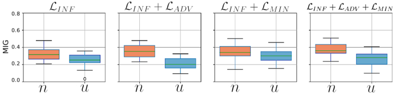
Figure 7: Box plots of the Mutual Information Gap (MIG) for each disentanglement objective for the negation and uncertainty factors computed on the Yelp test set.

					+$\mathcal{L}_{\mathrm{INF}}$+$\mathcal{L}_{\mathrm{ADV}}$
		+$\mathcal{L}_{\mathrm{INF}}$			+$\mathcal{L}_{\mathrm{MIN}}$
Factor	Pass	P	R	F1	P	R	F1
Neg	1	0.962	0.939	0.950	0.960	0.942	0.951
	2	0.932	0.887	0.908	0.944	0.907	0.924
Unc	1	0.975	0.955	0.965	0.982	0.950	0.965
	2	0.898	0.900	0.899	0.933	0.894	0.912

Table 17: Consistency of the decoder with the ground-truth values of negation and uncertainty evaluated on the SFU+Yelp test set. Pass 1 refers to the predictions from the original inputs. Pass 2 refers to the predictions from the re-encoded reconstructions. Pass 1 can be considered an upper bound on the performance of pass 2.

+$\mathcal{L}_{\mathrm{INF}}$ +$\mathcal{L}_{\mathrm{INF}}$ +$\mathcal{L}_{\mathrm{INF}}$+$\mathcal{L}_{\mathrm{ADV}}$ $\mathcal{L}_{\mathrm{ELBO}}$ +$\mathcal{L}_{\mathrm{INF}}$ +$\mathcal{L}_{\mathrm{ADV}}$ +$\mathcal{L}_{\mathrm{MIN}}$ +$\mathcal{L}_{\mathrm{MIN}}$ $u$ $c$ $u$ $c$ $u$ $c$ $u$ $c$ $u$ $c$ $n$ 0.090 0.003 0.135 0.001 0.164 0.012 0.110 0.006 0.123 0.002 ($\pm 0.013$) ($\pm 0.047$) ($\pm 0.038$) ($\pm 0.034$) ($\pm 0.028$) $u$ - 0.001 - 0.003 - 0.003 - 0.004 - 0.010 ($\pm 0.023$) ($\pm 0.042$) ($\pm 0.047$) ($\pm 0.040$) ($\pm 0.036$)

Table 18: Pearson’s correlation coefficients between each pair of latent representations across models on SFU+Yelp. As the content space is 62-dimensional, we compute the correlation coefficient between each dimension and report the mean and standard deviation.

						+$\mathcal{L}_{\mathrm{INF}}$
				+$\mathcal{L}_{\mathrm{INF}}$	+$\mathcal{L}_{\mathrm{INF}}$	+$\mathcal{L}_{\mathrm{ADV}}$
		$\mathcal{L}_{\mathrm{ELBO}}$	+$\mathcal{L}_{\mathrm{INF}}$	+$\mathcal{L}_{\mathrm{ADV}}$	+$\mathcal{L}_{\mathrm{MIN}}$	+$\mathcal{L}_{\mathrm{MIN}}$
BLEU	Train	0.805	0.786	0.793	0.786	0.796
	Dev	0.492	0.382	0.394	0.383	0.398
	Test	0.400	0.298	0.309	0.300	0.315
PPL	Train	52.7	54.8	53.3	54.1	53.7
	Dev	75.9	76.9	76.2	77.4	76.5
	Test	106.2	105.9	106.0	106.7	105.5

Table 19: Reconstruction self-BLEU and reconstruction perplexity (PPL) on each SFU+Yelp data split. Perplexity is computed using GPT-2.

D.2 Example Reconstructions

Input my jack and coke was seriously lacking. top brie and lobster was seriously lacking. Recon my pastrami and swiss was totally lacking. the camarones and coke was totally lacking. Input plus the dude didn’t even know how to work the computer. unfortunately the managers didn’t do too enough to compliment the computer. Recon unfortunately the women didn’t even know how to honor the experience. plus the baristas didn’t even know how to control the language. Input the service was great and would gladly go back. the service was great and would easily go back. Recon the service was exceptional and would probably go back. the service was great and would certainly go back. Input she could not and would not explain herself. she could not and would not explain herself. Recon she could not and would not respond herself. she could apologize and would not introduce herself.

Table 20: Example reconstructions decoded by the INF+ADV+MI model from the SFU+Yelp test set.

D.3 Controlled Generation

Table 21 reports the accuracies of attribute transfer on the SFU+Yelp test set. As reported for SFU+Amazon above, attribute transfer works well only when it is not necessary for the model to introduce additional tokens.

Transfer direction	Accuracy
pos $\rightarrow$ neg	0.38
neg $\rightarrow$ pos	0.87
cer $\rightarrow$ unc	0.36
unc $\rightarrow$ cer	0.86

Table 21: Attribute inversion accuracies by factor and direction of transfer using the $\mathcal{L}_{\mathrm{INF}}$+$\mathcal{L}_{\mathrm{ADV}}$+$\mathcal{L}_{\mathrm{MIN}}$ model on the SFU+Yelp test set.

Neg i totally agree but the way he said it was very arrogant. i even complained but the way but said it was not helpful. i will definitely come back for that and the singapore noodles. i absolutely never come back for that i ordered singapore noodles. overall i was not impressed and regret going. overall i was very impressed and recommended going. Unc we couldn’t wait till he was gone. we don’t wait till he was gone. room was very adequate quiet and clean. room would seemed quiet quiet and sanitary. the ending is as it should be. the ending is as it must be.

Table 22: Successful inversions of negation and uncertainty on the SFU+Yelp test set. Inputs are in standard font and reconstructions are in italics. bold tokens indicate negation/uncertainty cues.

Appendix E Implementation Details

We implement our model in PyTorch (Paszke et al., 2017). The encoder is a BiLSTM with 2 hidden layers and hidden size 256. The decoder is a 2 layer LSTM with hidden size 256. Embeddings for both the encoder and decoder are of size 256 and are randomly initialized and learned during training. The encoder and decoder use both word dropout and hidden layer dropout between LSTM layers, with a dropout probability of 0.5. We also use teacher forcing when training the decoder, with a probability of using the true previous token set to 0.5. We trained each model for 20 epochs with a batch size of 128 and the ADAM optimizer (Kingma and Ba, 2015) with a learning rate of $3\cdot 10^{-4}$. Training took around 6.5 hours for each model on one Tesla v100 with 16GB of VRAM.

The latent space classifiers for the INF objective and the adversarial classifiers for the ADV objective both used a single linear layer with sigmoid activation. The adversarial classifiers were trained with a separate ADAM optimizer with learning rate of $3\cdot 10^{-4}$. For MI estimation as part of the MIN objective we used the code released alongside the CLUB paper (Cheng et al., 2020a) . For training the approximation network, we again use an ADAM optimizer with learning rate $5\cdot 10^{-4}$.

All hyperparameter weights were tuned by hand. We weight the KL divergence term of each latent space separately as follows: $\beta_{c}=0.01,~{}\beta_{n}=\beta_{u}=0.005$. We experimented with both higher KL weights and KL annealing schedules, but found that they did not improve disentanglement and higher weights tended to negatively impact reconstruction ability. For the individual objectives, we set the following weights: $\lambda_{INF}=1.0,~{}\lambda_{ADV}=1.0,~{}\lambda_{MIN}=0.01$. While we found the model relatively robust to different values of $\lambda_{INF}$ and $\lambda_{ADV}$, the MIN objective was found to be quite sensitive to even small changes of both $\lambda_{MIN}$ and the learning rate of the MI approximation network.

E.1 Mutual Information Gap

The Mutual Information Gap (MIG) is the difference in MI between the top-2 latent variables $\ell_{\{i,j\}}$ with respect to a given generative factor $k$, normalized to lie in $[0,1]$, with higher values indicating a greater degree of disentanglement.

$$\text{MIG}_{k}=\frac{1}{H[k]}\left(I({\bf z}^{(\ell_{i})};k)-\max_{j\neq i}~{}I({\bf z}^{(\ell_{j})};k)\right)$$ (15)

where $\ell_{i}=\text{argmax}_{i^{\prime}}~{}I({\bf z}^{(\ell_{i^{\prime}})};k)$ is the latent space with the highest MI with the generative factor. We estimate the MI between latent representations and labels using the method proposed by Ross (2014), implemeted using mutual_info_classif in scikit-learn Pedregosa et al. (2011) using 30 resamples from the predicted latent distributions for each example.

Appendix F Ethical Considerations

This work is foundational NLP research on semantics, and as such we do not foresee any immediate risks, ethical or otherwise. However, representation learning may be used as part of many downstream NLP tasks such as information extraction, classification, and natural language generation, which might be used for harmful surveillance, discrimination, and misinformation.

The SFU, Amazon, and Yelp datasets used in this work do not attach unique identifiers such as user IDs or names to data instances such that the original authors might be identifiable. A manual review of a small random subset of the data did not reveal any overtly identifiable or harmful information within the text.

References

- Adel and Schütze (2017) Heike Adel and Hinrich Schütze. 2017. Exploring different dimensions of attention for uncertainty detection. In Proceedings of the 15th Conference of the European Chapter of the Association for Computational Linguistics: Volume 1, Long Papers, pages 22–34, Valencia, Spain. Association for Computational Linguistics.
- Balasubramanian et al. (2021) Vikash Balasubramanian, Ivan Kobyzev, Hareesh Bahuleyan, Ilya Shapiro, and Olga Vechtomova. 2021. Polarized-VAE: Proximity based disentangled representation learning for text generation. In Proceedings of the 16th Conference of the European Chapter of the Association for Computational Linguistics: Main Volume, pages 416–423, Online. Association for Computational Linguistics.
- Bao et al. (2019) Yu Bao, Hao Zhou, Shujian Huang, Lei Li, Lili Mou, Olga Vechtomova, Xin-yu Dai, and Jiajun Chen. 2019. Generating sentences from disentangled syntactic and semantic spaces. In Proceedings of the 57th Annual Meeting of the Association for Computational Linguistics, pages 6008–6019, Florence, Italy. Association for Computational Linguistics.
- Barnes et al. (2021) Jeremy Barnes, Erik Velldal, and Lilja Øvrelid. 2021. Improving sentiment analysis with multi-task learning of negation. Natural Language Engineering, 27(2):249–269.
- Benamara et al. (2012) Farah Benamara, Baptiste Chardon, Yannick Mathieu, Vladimir Popescu, and Nicholas Asher. 2012. How do negation and modality impact on opinions? In Proceedings of the Workshop on Extra-Propositional Aspects of Meaning in Computational Linguistics, pages 10–18, Jeju, Republic of Korea. Association for Computational Linguistics.
- Bengio et al. (2013) Y. Bengio, A. Courville, and P. Vincent. 2013. Representation learning: A review and new perspectives. IEEE Transactions on Pattern Analysis and Machine Intelligence, 35(8):1798–1828.
- Bosc and Vincent (2020) Tom Bosc and Pascal Vincent. 2020. Do sequence-to-sequence VAEs learn global features of sentences? In Proceedings of the 2020 Conference on Empirical Methods in Natural Language Processing (EMNLP), page 4296–4318. Association for Computational Linguistics.
- Bowman et al. (2016) Samuel R. Bowman, Luke Vilnis, Oriol Vinyals, Andrew Dai, Rafal Jozefowicz, and Samy Bengio. 2016. Generating sentences from a continuous space. In Proceedings of The 20th SIGNLL Conference on Computational Natural Language Learning, pages 10–21, Berlin, Germany. Association for Computational Linguistics.
- Cann (1993a) Ronnie Cann. 1993a. 3.3.1 Negation, Cambridge Textbooks in Linguistics, page 60–61. Cambridge University Press.
- Cann (1993b) Ronnie Cann. 1993b. 9.3.1 Simple modality, Cambridge Textbooks in Linguistics, page 270–276. Cambridge University Press.
- Chen and Batmanghelich (2020) Junxiang Chen and Kayhan Batmanghelich. 2020. Weakly supervised disentanglement by pairwise similarities. Proceedings of the … AAAI Conference on Artificial Intelligence. AAAI Conference on Artificial Intelligence, 34(4):3495–3502.
- Chen et al. (2018) Ricky T. Q. Chen, Xuechen Li, Roger Grosse, and David Duvenaud. 2018. Isolating sources of disentanglement in VAEs. In Proceedings of the 32nd International Conference on Neural Information Processing Systems, NIPS’18, page 2615–2625. Curran Associates Inc.
- Cheng et al. (2020a) Pengyu Cheng, Weituo Hao, Shuyang Dai, Jiachang Liu, Zhe Gan, and Lawrence Carin. 2020a. CLUB: A Contrastive Log-ratio Upper Bound of mutual information. In International Conference on Machine Learning, page 1779–1788. PMLR.
- Cheng et al. (2020b) Pengyu Cheng, Martin Renqiang Min, Dinghan Shen, Christopher Malon, Yizhe Zhang, Yitong Li, and Lawrence Carin. 2020b. Improving disentangled text representation learning with information-theoretic guidance. In Proceedings of the 58th Annual Meeting of the Association for Computational Linguistics, pages 7530–7541, Online. Association for Computational Linguistics.
- Choy and Chong (2018) Murphy Choy and Mark Chong. 2018. Seeing through misinformation: A framework for identifying fake online news. arXiv preprint arXiv:1804.03508.
- Colombo et al. (2021) Pierre Colombo, Pablo Piantanida, and Chloé Clavel. 2021. A novel estimator of mutual information for learning to disentangle textual representations. In Proceedings of the 59th Annual Meeting of the Association for Computational Linguistics and the 11th International Joint Conference on Natural Language Processing (Volume 1: Long Papers), pages 6539–6550, Online. Association for Computational Linguistics.
- Dupont (2018) Emilien Dupont. 2018. Learning disentangled joint continuous and discrete representations. In Proceedings of the 32nd International Conference on Neural Information Processing Systems, NIPS’18, page 708–718. Curran Associates Inc.
- Eastwood and Williams (2018) Cian Eastwood and Christopher K. I. Williams. 2018. A framework for the quantitative evaluation of disentangled representations. In International Conference on Learning Representations.
- Fancellu et al. (2016) Federico Fancellu, Adam Lopez, and Bonnie Webber. 2016. Neural networks for negation scope detection. In Proceedings of the 54th Annual Meeting of the Association for Computational Linguistics (Volume 1: Long Papers), page 495–504. Association for Computational Linguistics.
- Farkas et al. (2010) Richárd Farkas, Veronika Vincze, György Móra, János Csirik, and György Szarvas. 2010. The conll-2010 shared task: learning to detect hedges and their scope in natural language text. In Proceedings of the Fourteenth Conference on Computational Natural Language Learning—Shared Task, pages 1–12.
- Fu et al. (2018) Zhenxin Fu, Xiaoye Tan, Nanyun Peng, Dongyan Zhao, and Rui Yan. 2018. Style transfer in text: Exploration and evaluation. In AAAI Conference on Artificial Intelligence.
- Higgins et al. (2018) Irina Higgins, David Amos, David Pfau, Sebastien Racaniere, Loic Matthey, Danilo Rezende, and Alexander Lerchner. 2018. Towards a Definition of Disentangled Representations. arXiv:1812.02230 [cs, stat]. ArXiv: 1812.02230.
- Higgins et al. (2016) Irina Higgins, Loic Matthey, Arka Pal, Christopher Burgess, Xavier Glorot, Matthew Botvinick, Shakir Mohamed, and Alexander Lerchner. 2016. beta-VAE: Learning basic visual concepts with a constrained variational framework. In International Conference on Learning Representations.
- Hu et al. (2017) Zhiting Hu, Zichao Yang, Xiaodan Liang, Ruslan Salakhutdinov, and Eric P. Xing. 2017. Toward controlled generation of text. In International Conference on Machine Learning, page 1587–1596. PMLR.
- Jang et al. (2017) Eric Jang, Shixiang Gu, and Ben Poole. 2017. Categorical reparameterization with Gumbel-softmax. In 5th International Conference on Learning Representations, ICLR 2017, Toulon, France, April 24-26, 2017, Conference Track Proceedings. OpenReview.net.
- Jiménez-Zafra et al. (2020) Salud María Jiménez-Zafra, Roser Morante, Eduardo Blanco, María Teresa Martín Valdivia, and L. Alfonso Ureña López. 2020. Detecting negation cues and scopes in Spanish. In Proceedings of the 12th Language Resources and Evaluation Conference, pages 6902–6911, Marseille, France. European Language Resources Association.
- Jiménez-Zafra et al. (2018) Salud María Jiménez-Zafra, Mariona Taulé, M Teresa Martín-Valdivia, L Alfonso Urena-López, and M Antónia Martí. 2018. SFU review SP-NEG: a Spanish corpus annotated with negation for sentiment analysis. a typology of negation patterns. Language Resources and Evaluation, 52(2):533–569.
- John et al. (2019) Vineet John, Lili Mou, Hareesh Bahuleyan, and Olga Vechtomova. 2019. Disentangled representation learning for non-parallel text style transfer. In Proceedings of the 57th Annual Meeting of the Association for Computational Linguistics, pages 424–434, Florence, Italy. Association for Computational Linguistics.
- Khandelwal and Sawant (2020) Aditya Khandelwal and Suraj Sawant. 2020. NegBERT: A transfer learning approach for negation detection and scope resolution. In Proceedings of the 12th Language Resources and Evaluation Conference, page 5739–5748. European Language Resources Association.
- Kilicoglu et al. (2017) Halil Kilicoglu, Graciela Rosemblat, and Thomas C. Rindflesch. 2017. Assigning factuality values to semantic relations extracted from biomedical research literature. PLOS ONE, 12(7):e0179926.
- Kingma and Ba (2015) Diederik P. Kingma and Jimmy Ba. 2015. Adam: A method for stochastic optimization. In 3rd International Conference on Learning Representations, ICLR 2015, San Diego, CA, USA, May 7-9, 2015, Conference Track Proceedings.
- Kingma and Welling (2014) Diederik P. Kingma and Max Welling. 2014. Auto-encoding variational bayes. In 2nd International Conference on Learning Representations, ICLR 2014, Banff, AB, Canada, April 14-16, 2014, Conference Track Proceedings.
- Konstantinova et al. (2012) Natalia Konstantinova, Sheila C.M. de Sousa, Noa P. Cruz, Manuel J. Maña, Maite Taboada, and Ruslan Mitkov. 2012. A review corpus annotated for negation, speculation and their scope. In Proceedings of the Eighth International Conference on Language Resources and Evaluation (LREC’12), pages 3190–3195, Istanbul, Turkey. European Language Resources Association (ELRA).
- Lazib et al. (2019) Lydia Lazib, Yanyan Zhao, Bing Qin, and Ting Liu. 2019. Negation scope detection with recurrent neural networks models in review texts. International Journal of High Performance Computing and Networking, 13(2):211–221.
- Li and Lu (2018) Hao Li and Wei Lu. 2018. Learning with structured representations for negation scope extraction. In Proceedings of the 56th Annual Meeting of the Association for Computational Linguistics (Volume 2: Short Papers), page 533–539. Association for Computational Linguistics.
- Lin et al. (2020) Chen Lin, Steven Bethard, Dmitriy Dligach, Farig Sadeque, Guergana Savova, and Timothy A. Miller. 2020. Does BERT need domain adaptation for clinical negation detection? Journal of the American Medical Informatics Association, 27(4):584–591.
- Logeswaran et al. (2018) Lajanugen Logeswaran, Honglak Lee, and Samy Bengio. 2018. Content preserving text generation with attribute controls. In Advances in Neural Information Processing Systems 31: Annual Conference on Neural Information Processing Systems 2018, NeurIPS 2018, December 3-8, 2018, Montréal, Canada, pages 5108–5118.
- Maynez et al. (2020) Joshua Maynez, Shashi Narayan, Bernd Bohnet, and Ryan McDonald. 2020. On faithfulness and factuality in abstractive summarization. In Proceedings of the 58th Annual Meeting of the Association for Computational Linguistics, page 1906–1919. Association for Computational Linguistics.
- Paszke et al. (2017) Adam Paszke, Sam Gross, Soumith Chintala, Gregory Chanan, Edward Yang, Zachary DeVito, Zeming Lin, Alban Desmaison, Luca Antiga, and Adam Lerer. 2017. Automatic differentiation in PyTorch.
- Pedregosa et al. (2011) Fabian Pedregosa, Gaël Varoquaux, Alexandre Gramfort, Vincent Michel, Bertrand Thirion, Olivier Grisel, Mathieu Blondel, Peter Prettenhofer, Ron Weiss, Vincent Dubourg, Jake VanderPlas, Alexandre Passos, David Cournapeau, Matthieu Brucher, Matthieu Perrot, and Edouard Duchesnay. 2011. Scikit-learn: Machine learning in python. J. Mach. Learn. Res., 12:2825–2830.
- Qian et al. (2016) Zhong Qian, Peifeng Li, Qiaoming Zhu, Guodong Zhou, Zhunchen Luo, and Wei Luo. 2016. Speculation and negation scope detection via convolutional neural networks. In Proceedings of the 2016 Conference on Empirical Methods in Natural Language Processing, EMNLP 2016, Austin, Texas, USA, November 1-4, 2016, pages 815–825. The Association for Computational Linguistics.
- Radford et al. (2019) Alec Radford, Jeffrey Wu, Rewon Child, David Luan, Dario Amodei, Ilya Sutskever, et al. 2019. Language models are unsupervised multitask learners. OpenAI blog, 1(8):9.
- Ren et al. (2018) Yafeng Ren, Hao Fei, and Qiong Peng. 2018. Detecting the scope of negation and speculation in biomedical texts by using recursive neural network. In IEEE International Conference on Bioinformatics and Biomedicine, BIBM 2018, Madrid, Spain, December 3-6, 2018, pages 739–742. IEEE Computer Society.
- Ribeiro et al. (2020) Marco Tulio Ribeiro, Tongshuang Wu, Carlos Guestrin, and Sameer Singh. 2020. Beyond accuracy: Behavioral testing of NLP models with CheckList. In Proceedings of the 58th Annual Meeting of the Association for Computational Linguistics, pages 4902–4912, Online. Association for Computational Linguistics.
- Ross (2014) Brian C. Ross. 2014. Mutual information between discrete and continuous data sets. PLOS ONE, 9(2):e87357.
- Rubin (2007) Victoria L. Rubin. 2007. Stating with certainty or stating with doubt: Intercoder reliability results for manual annotation of epistemically modalized statements. In Human Language Technologies 2007: The Conference of the North American Chapter of the Association for Computational Linguistics; Companion Volume, Short Papers, pages 141–144, Rochester, New York. Association for Computational Linguistics.
- Saurí and Pustejovsky (2009) Roser Saurí and James Pustejovsky. 2009. Factbank: a corpus annotated with event factuality. Lang. Resour. Evaluation, 43(3):227–268.
- Shu et al. (2019) Rui Shu, Yining Chen, Abhishek Kumar, Stefano Ermon, and Ben Poole. 2019. Weakly supervised disentanglement with guarantees. In International Conference on Learning Representations.
- Stenetorp et al. (2012) Pontus Stenetorp, Sampo Pyysalo, Tomoko Ohta, Sophia Ananiadou, and Jun’ichi Tsujii. 2012. Bridging the gap between scope-based and event-based negation/speculation annotations: A bridge not too far. In Proceedings of the Workshop on Extra-Propositional Aspects of Meaning in Computational Linguistics, page 47–56. Association for Computational Linguistics.
- Thompson et al. (2017) Paul Thompson, Raheel Nawaz, John McNaught, and Sophia Ananiadou. 2017. Enriching news events with meta-knowledge information. Lang. Resour. Evaluation, 51(2):409–438.
- Van der Maaten and Hinton (2008) Laurens Van der Maaten and Geoffrey Hinton. 2008. Visualizing data using t-SNE. Journal of machine learning research, 9(11).
- Vincze et al. (2008) Veronika Vincze, György Szarvas, Richárd Farkas, György Móra, and János Csirik. 2008. The bioscope corpus: biomedical texts annotated for uncertainty, negation and their scopes. BMC Bioinform., 9(S-11).
- Wiegand et al. (2010) Michael Wiegand, Alexandra Balahur, Benjamin Roth, Dietrich Klakow, and Andrés Montoyo. 2010. A survey on the role of negation in sentiment analysis. In Proceedings of the Workshop on Negation and Speculation in Natural Language Processing, NeSp-NLP@ACL 2010, Uppsala, Sweden, July 10, 2010, pages 60–68. University of Antwerp.
- Yang et al. (2016) Zi Yang, Yue Zhou, and Eric Nyberg. 2016. Learning to answer biomedical questions: OAQA at BioASQ 4B. In Proceedings of the Fourth BioASQ workshop, pages 23–37, Berlin, Germany. Association for Computational Linguistics.
- Yatskar (2019) Mark Yatskar. 2019. A qualitative comparison of CoQA, SQuAD 2.0 and QuAC. In Proceedings of the 2019 Conference of the North American Chapter of the Association for Computational Linguistics: Human Language Technologies, Volume 1 (Long and Short Papers), pages 2318–2323, Minneapolis, Minnesota. Association for Computational Linguistics.
- Zerva (2019) Chrysoula Zerva. 2019. Automatic Identification of Textual Uncertainty. Ph.D. thesis, University of Manchester.
- Zhao and Bethard (2020) Yiyun Zhao and Steven Bethard. 2020. How does BERT’s attention change when you fine-tune? an analysis methodology and a case study in negation scope. In Proceedings of the 58th Annual Meeting of the Association for Computational Linguistics, pages 4729–4747, Online. Association for Computational Linguistics.