Preconditioned Least-Squares Petrov–Galerkin Reduced Order Models

Abstract

In this paper, we introduce a methodology for improving the accuracy and efficiency of reduced-order models (ROMs) constructed using the least-squares Petrov–Galerkin (LSPG) projection method through the introduction of preconditioning. Unlike prior related work, which focuses on preconditioning the linear systems arising within the ROM numerical solution procedure to improve linear solver performance, our approach leverages a preconditioning matrix directly within the minimization problem underlying the LSPG formulation. Applying preconditioning in this way has the potential to improve ROM accuracy for several reasons. First, preconditioning the LSPG formulation changes the norm defining the residual minimization, which can improve the residual-based stability constant bounding the ROM solution’s error. The incorporation of a preconditioner into the LSPG formulation can have the additional effect of scaling the components of the residual being minimized to make them roughly of the same magnitude, which can be beneficial when applying the LSPG method to problems with disparate scales (e.g., dimensional equations, multi-physics problems). Importantly, we demonstrate that an ‘ideal preconditioned’ LSPG ROM (a ROM in which the preconditioner is the inverse of the Jacobian of its corresponding full order model) emulates projection of the full order model solution increment onto the reduced basis. This quantity defines a lower bound on the error of a ROM solution for a given reduced basis. By designing preconditioners that approximate the Jacobian inverse—as is common in designing preconditioners for solving linear systems—it is possible to obtain a ROM whose error approaches this lower bound. The proposed approach is evaluated on several mechanical and thermo-mechanical problems implemented within the Albany HPC code and run in the predictive regime, with prediction across material parameter space. We demonstrate numerically that the introduction of simple Jacobi, Gauss-Seidel and ILU preconditioners into the Proper Orthogonal Decomposition (POD)/LSPG formulation reduces significantly the ROM solution error, the reduced Jacobian condition number, the number of nonlinear iterations required to reach convergence, and the wall time (thereby improving efficiency). Moreover, our numerical results reveal that the introduction of preconditioning can deliver a robust and accurate solution for test cases in which the unpreconditioned LSPG method fails to converge.

Keywords: Reduced order model (ROM), proper orthogonal decomposition (POD), Least-squares Petrov–Galerkin (LSPG) projection, preconditioners, computational solid mechanics, mechanical, thermo-mechanical.

1 Introduction

Numerous modern-day science and engineering problems require the simulation of complex systems with tens of millions of unknowns. Despite improved algorithms and the availability of massively parallel computing resources, “high-fidelity” models are, in practice, often too computationally expensive for use in time-critical settings such as design, fast turnaround analysis and control. The situation is particularly grave in applications involving multi-query analyses (e.g., optimization, uncertainty quantification), which require simulations to be repeated many times to explore the design space or to properly characterize uncertainty. The necessary calculations can present an intractable computational burden even with the projected growth in computing power as we approach the exascale computing age.

Reduced-order modeling is a promising strategy for reducing the computational cost of such simulations while preserving high levels of fidelity. Reduced-order models (ROMs) are models constructed from high-fidelity simulations that retain the essential physics and dynamics of their corresponding full order models (FOMs), but have a much lower computational cost. Although some consider a data-fit or low-fidelity model a ROM, herein the term “reduced order model” refers to a projection-based ROM. In projection-based model reduction, the state variables are restricted to reside in a low-dimensional subspace, typically computed offline through a data-compression process performed on a set of snapshots collected from a high-fidelity simulation or physical experiment, followed by truncation. There are numerous approaches in the literature for computing a low-dimensional subspace e.g., Proper Orthogonal Decomposition (POD) [72, 41], Dynamic Mode Decomposition (DMD) [62, 68] balanced POD (BPOD) [61, 82], balanced truncation [37, 50], and the reduced basis method (RBM) [63, 80]. Herein, without loss of generality, we restrict attention to the POD approach for calculating the reduced bases due to its prevalence and simplicity. Once a reduced basis is computed, the ROM dynamical system is obtained by projecting the governing equations, or some discretized form of these equations, onto the low-dimensional subspace. For nonlinear problems, an additional approximation, referred to as “hyper-reduction”, is usually required to gain a computational speed-up. Since ROMs are, by construction, low-dimensional and inexpensive to evaluate, these models can enable real-time analysis and alleviate the computational burden posed by high-dimensional uncertainty quantification (UQ) problems critical to many applications.

In order to serve as a viable predictive tool, a ROM should possess certain fundamental mathematical properties, such as consistency (with respect to its corresponding high-fidelity model), stability (in space as well as in time), and convergence (to the solution of its corresponding high-fidelity model). Galerkin projection, the most popular approach, is considered continuous optimal, as the resulting ROM minimizes the time-continuous residual in the $l^{2}$ norm [15], and preserves problem structure [21, 22, 47] for certain classes of problems (e.g., Lagrangian dynamical systems). However, the method can give rise to nonphysical instabilities [60, 45, 13, 44, 12, 11, 10, 18] and inaccurate long-time responses [71, 55, 15]. Additionally, it lacks in general an a priori convergence guarantee [62]. The least-squares Petrov–Galerkin (LSPG) projection method has been proposed [17] to remedy some of these difficulties via symmetrization of the discrete Jacobian. This method performs projection at the level of the fully discrete partial differential equations (PDEs), i.e., after the PDEs have been discretized in space and time, and computes a solution that minimizes the $\ell^{2}$-norm of the time-discrete residual arising in each time step. This procedure ensures that adding basis vectors yields a monotonic decrease in the least-squares objective function defining the underlying minimization problem. The method can maintain efficiency through the incorporation of hyper-reduction approaches such as gappy POD [31], the discrete empirical interpolation method (DEIM) [25] or the Energy-Conserving mesh Sampling and Weighing (ECSW) method [33, 24, 32], introduced to maintain efficiency of the method for nonlinear problems. When combined with gappy POD, the LSPG approach is equivalent to the Gauss–Newton with approximated tensors (GNAT) method [18]. While LSPG projection does not necessarily guarantee a priori accuracy and stability, it has been shown numerically to possess better stability and accuracy properties than the Galerkin method for a variety of problems [17, 18, 75, 77, 76, 15]. We note that the LSPG method has been extended in the time domain [27, 57], to allow for nonlinear trial manifolds rather than linear trial subspaces [48], to operate in a domain-decomposition setting [40], and to account for physics-based constraints [67].

The aim of the present paper is to develop a methodology for improving the accuracy of ROMs constructed using the LSPG projection method for a wide range of applications through the introduction of preconditioning. As shown in [15], LSPG errors are subject to a stability constant that is dictated by the residual. The use of preconditioning within the LSPG formulation improves the conditioning of the system, which improves the stability constants. Intuitively, this aligns the $\ell^{2}$-norm of the residual more closely with the $\ell^{2}$-norm of the (time-local) state error. To motivate the main contributions of this paper, we first provide a brief overview of related work involving projection-based ROMs and preconditioning.

1.1 Overview of related work

The idea of preconditioning began to make an appearance within the model-reduction literature approximately a decade ago. The bulk of the literature on this subject falls into two categories, which we overview succinctly below.

The first category of methods are aimed at developing ROM-based preconditioners for high-fidelity models. In [19, 58], the authors present a novel class of ROM-based preconditioners for the iterative high-fidelity solution of transient parabolic and self-adjoint PDEs. The preconditioners are obtained by nesting appropriate projections of ROMs into the classical preconditioned Conjugate Gradient (CG) iteration within the FOM. Several authors explore the idea of developing a ROM-based preconditioner to speed-up the numerical solution of the pressure system arising in high-fidelity reservoir modeling [8, 43]. In [8], Astrid et al. employ ROM concepts to develop a new preconditioner to speed up the pressure solution during a two-stage preconditioning procedure in a fully implicit time-integration scheme within a high-fidelity reservoir simulator. In [43], Jiang introduces a ROM-based preconditioner within a stationary Richardson iteration for the pressure system in a similar high-fidelity reservoir simulation.

The second category of methods explore the idea of introducing a preconditioner within the ROM workflow to speed up the online evaluation of the ROM. This work is motivated by the observation that the repeated solution of linear systems, characterized by dense matrices, can be the main computational bottleneck in efficient scaling of ROMs [69]. Commonly, the linear systems arising within the ROM workflow are solved using direct methods. This approach can be reasonable for small ROMs, but for larger ROMs containing numerous parameters, it was shown in [30] that a direct method can be more expensive to solve than the original FOM. Preconditioned iterative methods have been developed for alleviating this difficulty. In [29] and [30], preconditioners that are precomputed in the offline stage of the model reduction are introduced into a reduced basis ROM formulation with and without the application of discrete empirical interpolation to handle the nonlinear terms in the ROM. These preconditioners are derived from preconditioners used in solving the FOM, and are shown to be more efficient than direct solvers for problems depending on a moderately large number of parameters. Singh et al. develop strategies for reusing preconditioners in projection-based model reduction algorithms for parametric [70] and non-parametric [69] ROMs to improve scalability of ROM solution over direct methods. These authors introduce a novel Sparse Approximate Inverse (SPAI) preconditioner for ROMs constructed via moment matching using the Bilinear Iterative Rational Krylov Algorithm (BIRKA) algorithm. These preconditioners are aimed at systems where the linear system may change substantially between nonlinear iterations, as happens with highly nonlinear problems. Several other authors consider preconditioners constructed using IRKA methods, for which the most computationally demanding part is the solution of linear shifted systems. The ROM matrices in this case are sparse. Ahmad et al. [6] propose variants of the IRKA that use preconditioned versions of the shifted BiCG algorithm, and develop a polynomial preconditioner that can simultaneously be applied to all shifted systems. The idea of updating incomplete factorization preconditioners within the IRKA approach is explored in [7]. The use of randomized matrices to construct preconditioners for ROMs has been studied recently by several authors [83, 9]. In [83], the authors propose to use randomized linear algebra for the efficient construction of a preconditioner by interpolation of matrix inverse. It is shown that, in addition to improving the online performance of a given ROM, these preconditioners can be also used to improve the quality of residual-based error estimates in the context of the reduced basis method. Building on [83], Balabanov [9] addresses the efficient construction (using random sketching) of parameter-dependent preconditioners that can be used to improve the quality of Galerkin projections or for effective error certification for reduced basis and POD ROMs with ill-conditioned operators.

It is worthwhile to remark that the idea of preconditioning an LSPG ROM is related to several other recently-introduced methodologies for improving ROM accuracy, namely the idea of scaling the ROM residual prior to its minimization and the idea of modifying the norm in which the residual is minimized. In [81], Washabaugh proposed an approach for improving the accuracy of ROMs for systems of PDEs in which different variables have drastically different scales (e.g., applications where dimensional equations are employed). Specifically, it was shown in this reference that scaling the ROM residual to get all the equations to be roughly the same order of magnitude (equivalent to the application of a diagonal preconditioner) can result in more accurate ROMs. In a similar vein, it was demonstrated in [26] that normalizing snapshot data prior to computing POD modes in order to remove dimensional effects increases numerical robustness of ROMs for hypersonic aerodynamic simulations, especially in cases with non-equilibrium thermo-chemical effects. More recently, in [56], Parish and Rizzi developed a set of dimensionally-consistent inner products and demonstrated that these inner products have a positive impact on both Galerkin and LSPG ROMs with application to the compressible Euler equations. In [28], Collins et al. examined an optimal test basis for LSPG ROMs that are obtained by solving an adjoint-like system, which transforms the residual error minimization problem to be equivalent to a least-squares state error minimization problem. The resulting test functions can be seen as incorporating the action of a preconditioner matrix that approximates the inverse of the Jacobian matrix from a ROM’s corresponding FOM. In [5], Abgrall et al. proposed a residual minimization model reduction approach, in which the norm in which the residual is minimized is the $L^{1}$ norm. If the resulting $L^{1}$ residual minimization is solved iteratively using reweighted least-squares, the procedure can be interpreted as a least-squares solve.

1.2 Contributions and organization

A distinguishing feature of the present work that differentiates it from most of the references described above is the premise that the introduction of a preconditioner into the LSPG formulation can not only lead to performance gains (by reducing the condition number of the reduced Jacobian), but can actually improve a ROM’s accuracy. Unlike prior work, e.g., [30, 29, 69], the idea herein is not to simply precondition the linear systems arising within the LSPG algorithm to improve linear solver performance, but rather to insert a preconditioner matrix directly into the minimization problem underlying the LSPG formulation. Doing this has the effect of changing the norm defining the residual minimization problem underlying the LSPG method, which can improve the residual-based stability constant bounding the method’s error. We additionally demonstrate that:

• an ideal preconditioned LSPG ROM (a ROM in which the preconditioner is the inverse of the Jacobian of its corresponding FOM) emulates projection of the FOM solution increment onto the reduced basis, which defines a lower bound on the error of a ROM for a given reduced basis;

• it is possible to obtain a ROM whose error approaches this lower bound by improving the quality of the preconditioner employed within the LSPG formulation;

• the addition of certain preconditioners into the LSPG formulation can have the effect of scaling the components of the residual being minimized to make them roughly of the same magnitude, which can minimize bias and reduce the number of nonlinear iterations required for convergence when applying the LSPG method to problems with disparate scales (e.g., dimensional PDEs, multi-physics problems);

• while our approach is not specifically based on preconditioning the linear systems arising within the LSPG iteration process, it has the effect of reducing the condition numbers of an LSPG ROM’s reduced Jacobians.

We evaluate the performance and predictive accuracy of several preconditioned POD/LSPG ROMs on one mechanical and two thermo-mechanical problems implemented within the open-source HPC multi-physics finite element code known as Albany [65]. We point out that the vast majority of the current ROM literature uses Galerkin projection for the reduction step of the ROM workflow when considering solids and structures [1, 79, 33, 24, 32, 20, 23]; herein, we demonstrate that the preconditioned LSPG method can also be effective for this class of problems. For the mechanical problem, we demonstrate that preconditioning is needed to obtain a convergent POD/LSPG ROM. For the thermo-mechanical problems, we demonstrate that, while it is possible to obtain a convergent unpreconditioned POD/LSPG ROM for certain basis dimensions, the addition of preconditioning reduces the error by between two and seven orders of magnitude, all while reducing the overall wall time by as much as $12\times$. The wall time improvements can be attributed to a preconditioner’s ability to reduce not only the condition number of the reduced Jacobians arising within the LSPG algorithm, but also the total number of nonlinear iterations required for ROM convergence.

The remainder of this paper is organized as follows. In Section 2, we provide an overview of the POD/LSPG approach to model reduction applied to a generic system of nonlinear algebraic equations, which might arise from the discretization of a PDE. We introduce the notion of preconditioning within the LSPG residual minimization problem in Section 3. We demonstrate that the use of a preconditioner has the effect of changing the norm in which the LSPG residual minimization problem is solved, and show that the use of an ideal preconditioner (the inverse of a Jacobian matrix in a particular Newton iteration) will lead to an $l^{2}$-optimal projection of the solution increment onto the reduced basis. In Section 4, we describe succinctly the Albany multi-physics finite element code and our implementation of model reduction capabilities within this code, including a partitioned/“blocking vector" approach for applying ROM Dirichlet boundary conditions within a finite element code that does not remove the constrained (Dirichlet) degrees of freedom from the global finite element system prior to performing its numerical solution. We study the performance of the proposed preconditioned LSPG ROMs in the context of several mechanical and thermo-mechanical solid mechanics problems in Section 5, demonstrating the efficacy of the proposed preconditioning strategy. Finally, conclusions are offered in Section 6.

2 Problem formulation

2.1 Full-order model

Since the methodology described herein can be applied to a wide range of FOMs arising in a variety of applications, let us consider the following generic system of nonlinear algebraic equations defining our FOM:

$$\bm{r}(\bm{w})=\bm{0}.$$ (1)

Here, $\bm{w}\in\mathbb{R}^{N}$ is the state vector and $\bm{r}:\mathbb{R}^{N}\rightarrow\mathbb{R}^{N}$ is the nonlinear residual operator. Systems of the form (1) are obtained by fully discretizing a set of governing PDEs using a spatial discretization method and, in the case of a dynamics problem, a time-integration scheme. Assuming we solve (1) using a (globalized) Newton’s method, the following sequence of solutions is generated:

$$\bm{J}^{(k)}\delta\bm{w}^{(k)} =-\bm{r}^{(k)},\quad k=1,\ldots,K,$$ (2)

$$\bm{w}^{(k)} =\bm{w}^{(k-1)}+\alpha_{k}\delta\bm{w}^{(k)}.$$

Here, $\bm{J}^{(k)}:=\frac{\partial\bm{r}}{\partial\bm{w}}\left(\bm{w}^{(k)}\right)\in\mathbb{R}^{N\times N}$ is the FOM Jacobian, $\bm{r}^{(k)}:=\bm{r}\left(\bm{w}^{(k)}\right)\in\mathbb{R}^{N}$ is the FOM residual, $\bm{w}^{(0)}$ is an initial guess for the solution, $\alpha_{k}\in\mathbb{R}$ is the step length (obtained using a line-search method, or set to one, as commonly done), and $K$ is the number of Newton iterations.

2.2 Reduced order models

Our task is to build a ROM for (1) using the projection-based model reduction approach. This approach consists of three steps:

1. calculation of a reduced basis,

2. projection of the governing equations (in our case, (1)) onto the subspace spanned by the reduced basis, and

3. hyper-reduction to handle efficiently the projection of the nonlinear terms.

We describe each of these steps succinctly in the following subsections. As mentioned earlier in the introduction, we restrict our attention herein to reduced bases calculated using the POD. The numerical implementation of the model reduction algorithms outlined in this section within the Albany multi-physics finite element code is discussed later, in Section 5.

2.2.1 Reduced basis calculation via the POD

The first step in the projection-based approach to model reduction is the calculation of a basis of reduced dimension $M\ll N$ (where $N$ denotes the number of degrees of freedom (dofs) in the full order model (1)) using the POD. The POD is a mathematical procedure that, given an ensemble of data and an inner product, denoted generically by $(\cdot,\cdot)$, constructs a basis for the ensemble that is optimal in the sense that it describes more energy (on average) of the ensemble in the chosen inner product than any other linear basis of the same dimension $M$. The ensemble $\{\bm{w}^{p}:p=1,\dots,P\}$ is typically a set of $P$ instantaneous snapshots of a numerical solution field, collected for $P$ values of a parameter of interest, or at $P$ different times. Following the so-called “method of snapshots" [72], given a snapshot matrix $\leavevmode\nobreak\ W:=[\leavevmode\nobreak\ w^{1},...,\leavevmode\nobreak\ w^{P}]\in\mathbb{R}^{N\times P}$, a POD basis $\bm{\Phi}_{M}$ of dimension $M\leq P$ is obtained by first computing the (thin) singular value decomposition (SVD)

$$\leavevmode\nobreak\ W=\leavevmode\nobreak\ U\leavevmode\nobreak\ \Sigma\leavevmode\nobreak\ V^{T},$$ (3)

where the left singular vector matrix $\leavevmode\nobreak\ U:=[\leavevmode\nobreak\ u^{1},...,\leavevmode\nobreak\ u^{P}]\in\mathbb{R}^{N\times P}$ is orthogonal ($\leavevmode\nobreak\ U^{T}\leavevmode\nobreak\ U=\leavevmode\nobreak\ I$), the diagonal singular value matrix $\leavevmode\nobreak\ \Sigma=\text{diag}(\sigma_{i})$ contains the ordered singular values $\sigma_{1}\geq\sigma_{2}\geq...\geq\sigma_{P}\geq 0$ of $\leavevmode\nobreak\ W$, and the right singular vector matrix $\leavevmode\nobreak\ V\in\mathbb{R}^{P\times P}$ is also orthogonal, like $\leavevmode\nobreak\ U$ ($\leavevmode\nobreak\ V^{T}\leavevmode\nobreak\ V=\leavevmode\nobreak\ I$). Given (3), the sought-after POD basis is obtained by selecting the first $M\leq P$ left singular vectors of $\leavevmode\nobreak\ W$:

$$\bm{\Phi}_{M}:=[u^{1},...,u^{P}]\in\mathbb{R}^{N\times M}.$$ (4)

It follows that $\bm{\Phi}_{M}$ has orthonormal columns and satisfies $\bm{\Phi}_{M}^{T}\bm{\Phi}_{M}=\leavevmode\nobreak\ I$.

Once $\bm{\Phi}_{M}$ is calculated, we approximate the solution to (1) by

$$\tilde{\bm{w}}={\bm{w}}_{0}+\bm{\Phi}_{M}\hat{\bm{w}}={\bm{w}}_{0}+\sum_{i=1}^{M}{\bm{\phi}}_{i}\hat{w}_{i}$$ (5)

where ${\bm{\phi}}_{i}:=\leavevmode\nobreak\ u^{i}$ for $i=1,...,M$, $\hat{\bm{w}}:=\left[\hat{w}_{1}\ \cdots\ \hat{w}_{M}\right]^{T}\in\mathbb{R}^{M}$ denote the generalized coordinates, and ${\bm{w}}_{0}\in\mathbb{R}^{N}$ denotes a reference solution, often taken to be the initial condition in the case of an unsteady simulation. Substituting the approximation (5) into (1) yields

$$\bm{r}({\bm{w}}_{0}+\bm{\Phi}_{M}\hat{\bm{w}})=\bm{0}.$$ (6)

(6) is a system of $N$ equations in $M$ unknowns $\hat{\bm{w}}$. As this is an over-determined system, it may not have a solution.

2.2.2 Least-Squares Petrov–Galerkin (LSPG) projection

As discussed earlier, the LSPG approach [17] to model reduction has shown some promise in mitigating the stability problems and other disadvantages of other approaches, e.g., the Galerkin projection method. In the LSPG approach, the ROM solution in (5) is obtained by solving the following least-squares optimization problem:

$${\hat{\bm{w}}}_{\text{PG}}\in\arg\min_{\bm{y}\in\mathbb{R}^{M}}\|\bm{r}({\bm{w}}_{0}+\bm{\Phi}_{M}\bm{y})\|_{2}^{2}.$$ (7)

Here, the approximate (Petrov–Galerkin) solution is ${\tilde{\bm{w}}}_{\text{PG}}:={\bm{w}}_{0}+\bm{\Phi}_{M}{\hat{\bm{w}}}_{\text{PG}}$. The name “LSPG" ROM comes from the observation that solving (7) amounts to solving a nonlinear least-squares problem. The two most popular approaches for this are the Gauss–Newton approach and the Levenberg–Marquardt (trust-region) method. Following the work of Carlberg et al. [18], we adopt the Gauss–Newton approach. This approach implies solving a sequence of linear least-squares problems of the form

$$\delta{\hat{\bm{w}}}_{\text{PG}}^{(k)}\in\arg\min_{\bm{y}\in\mathbb{R}^{M}}\|\bm{J}^{(k)}\bm{\Phi}_{M}\bm{y}+\bm{r}^{(k)}\|_{2}^{2},\quad k=1,\ldots,{K}_{\text{PG}},$$ (8)

$${\hat{\bm{w}}}_{\text{PG}}^{(k)}={\hat{\bm{w}}}_{\text{PG}}^{(k-1)}+\alpha_{k}\delta{\hat{\bm{w}}}_{\text{PG}}^{(k)},$$ (9)

$${\tilde{\bm{w}}}_{\text{PG}}^{(k)}={\bm{w}}_{0}+\bm{\Phi}_{M}{\hat{\bm{w}}}_{\text{PG}}^{(k-1)},$$ (10)

where ${K}_{\text{PG}}$ is the number of Gauss–Newton iterations. It can be shown that the approximation upon convergence is ${\tilde{\bm{w}}}_{\text{PG}}={\tilde{\bm{w}}}_{\text{PG}}^{({K}_{\text{PG}})}$ and ${\hat{\bm{w}}}_{\text{PG}}={\hat{\bm{w}}}_{\text{PG}}^{({K}_{\text{PG}})}$. Note that the normal equations for (8) take the form

$${\bm{J}}_{\text{PG}}^{(k)}\delta{\hat{\bm{w}}}_{\text{PG}}^{(k)}=-{\bm{r}}_{\text{PG}}^{(k)},\quad k=1,\ldots,{K}_{\text{PG}},$$ (11)

where

$${\bm{J}}_{\text{PG}}^{(k)}:={\bm{\Psi}_{M}^{(k)}}^{T}\bm{J}^{(k)}\bm{\Phi}_{M},\hskip 14.22636pt{\bm{r}}_{\text{PG}}^{(k)}:={\bm{\Psi}_{M}^{(k)}}^{T}\bm{r}^{(k)},$$ (12)

and

$$\bm{\Psi}_{M}^{(k)}:=\bm{J}^{(k)}\bm{\Phi}_{M}.$$ (13)

Equation (8) can be solved numerically using a variety of methods, including solving the normal equations (11), or by employing more numerically stable methods such as the QR decomposition and the SVD; see [18] for more details.

Remark 1. It is clear from (12) and (13) that LSPG projection can be interpreted as a Petrov–Galerkin process of the Newton iteration with trial basis $\bm{\Phi}_{M}$ and test basis $\bm{\Psi}_{M}^{(k)}$ defined in (13).

Remark 2. When Newton’s method is employed to solve the reduced state equations for the LSPG method, the ROM solution procedure can be viewed as minimizing at each iteration the error in the search direction:

$$\delta\hat{\bm{w}}\in\arg\min_{\bm{y}\in\mathbb{R}^{M}}\|\bm{\Phi}_{M}\bm{y}-\delta\bm{w}^{(k)}\|_{{\bm{\Theta}}}^{2}=\arg\min_{\bm{y}\in\mathbb{R}^{M}}\|\bm{\Phi}_{M}\bm{y}+{\bm{J}^{(k)}}^{-1}\bm{r}^{(k)}\|_{{\bm{\Theta}}}^{2},$$ (14)

where ${\bm{\Theta}}:={\bm{J}^{(k)}}^{T}\bm{J}^{(k)}$ and $||\mathbf{x}||_{{\bm{\Theta}}}:=\sqrt{\mathbf{x}^{T}{\bm{\Theta}}\mathbf{x}}$. Since ${\bm{\Theta}}$ is always a symmetric positive-definite matrix, the LSPG approach has the effect of symmetrizing the discrete ROM Jacobian. As shown in [17], when (14) is satisfied, the error measure $\|\bm{\Phi}_{M}\bm{y}-\delta\bm{w}^{(k)}\|_{{\bm{\Theta}}}$ decreases monotonically as vectors are added to the POD basis.

2.2.3 Hyper-reduction

The LSPG projection approach described in Section 2.2.2 is inefficient for nonlinear problems. This is because the solution of the ROM system requires algebraic operations that scale with the dimension of the original full order model $N$. This problem can be circumvented through the use of hyper-reduction. A number of hyper-reduction approaches have been proposed, including DEIM [25], “best points" interpolation [53, 54], collocation [49], gappy POD [31] and the ECSW method [33, 24, 32]. The basic idea behind these approaches is to compute the residual at some small number of points $q$ with $q\ll N$, encapsulated in a “sampling matrix" $\bm{Z}$. This set of $q$ points is typically referred to as the “sample mesh". The “sample mesh" is computed offline using a greedy algorithm following the notion of gappy data reconstruction [31], as described in detail in [18] and [16]. The LSPG projection approach combined with gappy POD hyper-reduction is equivalent to the GNAT method [18]. In this method, the nonlinear least-squares problem (7) is replaced with

$$\hat{\bm{w}}_{\text{GNAT}}\in\arg\min_{\bm{y}\in\mathbb{R}^{M}}\|(\bm{ZW})^{+}\bm{Z}\bm{r}({\bm{w}}_{0}+\bm{\Phi}_{M}\bm{y})\|_{2}^{2},$$ (15)

where $\bm{W}\in\mathbb{R}^{N\times M}$ is a reduced basis for the residual $\bm{r}$ and the ‘+’ symbol denotes the pseudo-inverse. It is straightforward to demonstrate that the Gauss–Newton iterations corresponding to (15) take the form

$$\delta\hat{\bm{w}}_{\text{GNAT}}^{(k)}\in\arg\min_{\bm{y}\in\mathbb{R}^{M}}\left|\left|(\bm{ZW}^{+})\bm{Z}\left[\bm{J}^{(k)}\bm{\Phi}_{M}\bm{y}+\bm{r}^{(k)}\right]\right|\right|_{2}^{2},\quad k=1,\ldots,K_{\text{GNAT}},$$ (16)

$$\hat{\bm{w}}_{\text{GNAT}}^{(k)}=\hat{\bm{w}}_{\text{GNAT}}^{(k-1)}+\alpha_{k}\delta\hat{\bm{w}}_{\text{GNAT}}^{(k)},$$ (17)

$$\tilde{\bm{w}}_{\text{GNAT}}^{(k)}={\bm{w}}_{0}+\bm{\Phi}_{M}\hat{\bm{w}}_{\text{GNAT}}^{(k-1)},$$ (18)

where $K_{\text{GNAT}}$ denotes the number of Gauss–Newton iterations. It is noted that the gappy POD approximation in (15) and (16) aims to approximate the entire residual and Jacobian (via least-squares approximation) rather than simply sub-sample those quantities.

3 Preconditioned reduced order models

Having overviewed our basic ROM workflow, we now introduce the concept of preconditioned ROMs to the general LSPG formulation described in Section 2.2.2. Let $\bm{M}\in\mathbb{R}^{N\times N}$ denote a non-singular preconditioner matrix. In the present work, a preconditioned LSPG ROM is obtained by inserting $\bm{M}$ into the least-squares optimization problem (7) to yield:

$${\hat{\bm{w}}}_{\text{PPG}}\in\arg\min_{\bm{y}\in\mathbb{R}^{M}}\|\bm{M}\bm{r}({\bm{w}}_{0}+\bm{\Phi}_{M}\bm{y})\|_{2}^{2},$$ (19)

where ${\hat{\bm{w}}}_{\text{PPG}}$ denotes the generalized coordinates of the preconditioned Petrov–Galerkin ROM. It is noted that $\bm{M}\bm{r}(\bm{w})=\bm{0}$ is equivalent to (1) provided $\bm{M}$ is non-singular.

Similar to the standard LSPG approach, if (19) is solved using a Gauss–Newton algorithm, one obtains the following sequence of linear least-squares problems:

$$\delta{\hat{\bm{w}}}_{\text{PPG}}^{(k)}\in\arg\min_{\bm{y}\in\mathbb{R}^{M}}\left|\left|\bm{M}^{(k)}\left(\bm{J}^{(k)}\bm{\Phi}_{M}\bm{y}+\bm{r}^{(k)}\right)\right|\right|_{2}^{2},\quad k=1,\ldots,{K}_{\text{PG}},$$ (20)

$${\hat{\bm{w}}}_{\text{PPG}}^{(k)}={\hat{\bm{w}}}_{\text{PPG}}^{(k-1)}+\alpha_{k}\delta{\hat{\bm{w}}}_{\text{PPG}}^{(k)},$$ (21)

$${\tilde{\bm{w}}}_{\text{PPG}}^{(k)}={\bm{w}}_{0}+\bm{\Phi}_{M}{\hat{\bm{w}}}_{\text{PPG}}^{(k-1)},$$ (22)

where ${K}_{\text{PPG}}$ is the number of Gauss–Newton iterations. In (20), the superscript $(k)$ has been added to $\bm{M}^{(k)}$ to indicated that, just like the Jacobian $\bm{J}^{(k)}$, the preconditioner may change in each Gauss–Newton iteration. We will assume that the sequence of preconditioners $\bm{M}^{(k)}$ is non-singular. The normal equations corresponding to (20) are

$${\bm{J}}_{\text{PPG}}^{(k)}\delta{\hat{\bm{w}}}_{\text{PPG}}^{(k)}=-{\bm{r}}_{\text{PPG}}^{(k)},\quad k=1,\ldots,{K}_{\text{PPG}}\;$$ (23)

where

$${\bm{J}}_{\text{PPG}}^{(k)}:=\bm{\Phi}_{M}^{T}(\bm{J}^{(k)})^{T}(\bm{M}^{(k)})^{T}\bm{M}^{(k)}\bm{J}^{(k)}\bm{\Phi}_{M},\hskip 14.22636pt{\bm{r}}_{\text{PPG}}^{(k)}:=\bm{\Phi}_{M}^{T}(\bm{J}^{(k)})^{T}(\bm{M}^{(k)})^{T}\bm{M}^{(k)}\bm{r}^{(k)}.$$ (24)

In the remainder of this section, we bring to light and discuss the implications of several important properties of preconditioned LSPG ROMs constructed via the approach described above.

Theorem 1.

An “ideal" preconditioned ROM (a ROM in which $\bm{M}^{(k)}={\bm{J}^{(k)}}^{-1}$ for each Gauss–Newton iteration $k$) emulates the projection of the FOM solution increment onto a given POD basis:

$$\delta\tilde{\bm{w}}^{(k)}=\bm{\Phi}_{M}\left(\bm{\Phi}_{M}^{T}\bm{\Phi}_{M}\right)^{-1}\bm{\Phi}_{M}^{T}\delta\bm{w}^{(k)}.$$ (25)

Since (25) is the upper limit on the ROM accuracy given a basis $\bm{\Phi}_{M}$, it follows that the most accurate ROM possible is realizable through the introduction of preconditioning.

Proof.

Assume $\bm{J}^{(k)}$ is full rank and let $\bm{M}^{(k)}={\bm{J}^{(k)}}^{-1}$. Substituting this $\bm{M}^{(k)}$ into (23) reduces these normal equations to

$$\bm{\Phi}_{M}^{T}\bm{\Phi}_{M}\delta{\hat{\bm{w}}}_{\text{PPG}}^{(k)}=-\bm{\Phi}_{M}^{T}{\bm{J}^{(k)}}^{-1}\bm{r}^{(k)},\quad k=1,\ldots,{K}_{\text{PPG}}\;.$$ (26)

Recognizing that the right-hand side of (26) contains the FOM solution increment $\delta\bm{w}^{(k)}=-{\bm{J}^{(k)}}^{-1}\bm{r}^{(k)}$, (26) is equivalent to

$$\delta{\hat{\bm{w}}}_{\text{PPG}}^{(k)}=(\bm{\Phi}_{M}^{T}\bm{\Phi}_{M})^{-1}\bm{\Phi}_{M}^{T}\delta\bm{w}^{(k)},\quad k=1,\ldots,{K}_{\text{PPG}}\;,$$ (27)

so that, from (5), $\delta\tilde{\bm{w}}^{(k)}$ is given by (25).

∎

Theorem 2.

Introducing preconditioning into the LSPG formulation as in (20) has the effect of modifying the norm ${\bm{\Theta}}$ in which the solution increment minimization is performed (14). For a generic non-singular preconditioner matrix $\bm{M}^{(k)}$, the LSPG ROM solution procedure can be can be viewed as minimizing at each iteration the error in the search direction (14) in the norm given by ${\bm{\Theta}}=(\bm{J}^{(k)})^{T}(\bm{M}^{(k)})^{T}\bm{M}^{(k)}\bm{J}^{(k)}$. For an ideal preconditioner ($\bm{M}^{(k)}={\bm{J}^{(k)}}^{-1}$), ${\bm{\Theta}}=\bm{I}$, which leads to an $l^{2}$-optimal projection of the solution increment $\delta\bm{w}^{(k)}$ onto the reduced basis $\bm{\Phi}_{M}$:

$$\delta{\hat{\bm{w}}}_{\text{PPG}}^{(k)}\in\arg\min_{\bm{y}\in\mathbb{R}^{M}}\|\bm{\Phi}_{M}\bm{y}-\delta\bm{w}^{(k)}\|_{2}^{2}$$ (28)

Proof.

It is straightforward to see that

$$\|\bm{M}^{(k)}\left(\bm{J}^{(k)}\bm{\Phi}_{M}\bm{y}+\bm{r}^{(k)}\right)\|_{2}^{2}=\|\bm{M}^{(k)}\bm{J}^{(k)}\left(\bm{\Phi}_{M}\bm{y}+{\bm{J}^{(k)}}^{-1}\bm{r}^{(k)}\right)\|_{2}^{2}=\|\bm{\Phi}_{M}\bm{y}+{\bm{J}^{(k)}}^{-1}\bm{r}^{(k)}\|_{{\bm{\Theta}}}^{2},$$ (29)

where ${\bm{\Theta}}=(\bm{J}^{(k)})^{T}(\bm{M}^{(k)})^{T}\bm{M}^{(k)}\bm{J}^{(k)}$. The claim follows immediately. Substituting $\bm{M}^{(k)}={\bm{J}^{(k)}}^{-1}$ and $\delta\bm{w}^{(k)}=-{\bm{J}^{(k)}}^{-1}\bm{r}^{(k)}$ into (29) gives (28). ∎

While selecting $\bm{M}^{(k)}={\bm{J}^{(k)}}^{-1}$ is infeasible in practice, an important corollary of Theorem 1 is that by selecting a preconditioner matrix that approximates ${\bm{J}^{(k)}}^{-1}$, it is possible to improve the accuracy of a given LSPG ROM, with the ROM solution approaching the most accurate ROM solution possible (for a given basis $\bm{\Phi}_{M}$) as $\bm{M}^{(k)}\to{\bm{J}^{(k)}}^{-1}$. Moreover, if $\bm{M}^{(k)}$ is selected such that $\text{cond}\left(\bm{M}^{(k)}\bm{J}^{(k)}\right)<\text{cond}\left(\bm{J}^{(k)}\right)$ (where $\text{cond}(\bm{A})$ denotes the condition number of a matrix $\bm{A}$), it is possible to improve the condition numbers of the reduced Jacobians (24) arising in the Gauss–Newton iteration process.

We end this section by remarking that there is an additional benefit of introducing a preconditioner into the LSPG formulation (7) as in (19). It has been observed [81, 26, 56] that minimizing the raw (unweighted) residual $\bm{r}$ can be problematic for systems of PDEs where different variables have drastically different magnitudes, which happens frequently in various applications where dimensional equations are employed. Residual components corresponding to certain variables can be very large compared to the residual components corresponding to other variables, thereby biasing the minimization procedure. As shown in [81, 26, 56], scaling the ROM residual to get all the equations to be roughly the same order of magnitude can remedy this problem. From (19), it is can be seen that the introduction of a preconditioner $\bm{M}$ can have the same effect.

4 Implementation in the Albany multi-physics finite element code

The preconditioned LSPG ROMs described herein have been implemented with a version of the Albany code base [3], described succinctly in this section. Albany is an open-source C++ object-oriented, parallel, unstructured-grid, implicit finite element code for solving general PDEs, developed using the “Agile Components" code development strategy [66] with mature modular libraries from the Trilinos [39] project. Over the years, Albany has hosted a number of science and engineering applications, including the Aeras global atmosphere code [73], the Albany Land-Ice (ALI) [78] ice sheet model solver, the Quantum Computer Aided Design (QCAD) [36] simulator, the ACE thermo-mechanical terrestrial model of Arctic coastal erosion [34], and the Laboratory for Computational Mechanics (LCM) [74, 52, 51] research code. This last project comprises Albany LCM and is specifically targeted at solid mechanics applications, such as the ones considered in this paper. A more detailed description of Albany, including a detailed description of its underlying design and the physics implemented therein, can be found in [65].

In the subsections below, we describe the main ingredients enabling the construction of preconditioned LSPG ROMs within the Albany code base. We present also a special partitioned/“blocking vector" approach for applying ROM Dirichlet boundary conditions within this code base, which does not remove the constrained dofs from the global finite element system prior to performing its numerical solution. This implementation is extensible to other finite element codes with similar boundary condition treatment.

4.1 The model reduction workflow in Albany

As described in Section 2.2, the basic workflow in building a ROM consists of three steps: calculation of a reduced basis, projection of the governing equations onto the reduced basis, and calculation of a sample mesh using hyper-reduction. The implementation of this workflow within Albany for a generic nonlinear problem is demonstrated in Algorithm 1.

Given: Albany, AlbanyRBGen, AlbanyMeshSample executables, and corresponding input files: fomInput.xml, reducedBasisInput.xml, meshReduceInput.xml, romInput.xml

# Run the full order model to get the snapshots

./Albany fomInput.xml

# Compute reduced basis (RBGen required)

./AlbanyRBGen reducedBasisInput.xml

# Compute sample nodes and reduced mesh

./AlbanyMeshSample meshReduceInput.xml

# Run the ROM with hyper-reduction (sample mesh)

./Albany romInput.xml

Algorithm 1 Albany model reduction workflow. Example input files can be found in the GitHub repository corresponding to this version of Albany [3], in the directory Albany-MOR_support_ends/tests/small/MOR/MOR_MechanicalCube.

First, the main Albany executable is run in FOM mode to collect the relevant snapshots for a given problem, which are written to an output Exodus file. Next, the reduced basis and sample mesh are calculated in Albany as a pre-processing step by utilities known as AlbanyRBGen and AlbanyMeshReduce, respectively, using data collected from a high-fidelity simulation. The AlbanyRBGen utility employs the RBGen module within the Anasazi package of Trilinos [2] to calculate a reduced basis $\bm{\Phi}_{M}$ using the POD algorithm outlined in Section 2.2.1. While it is possible to use AlbanyRBGen to generate a scalar POD basis (i.e., a separate POD basis built for each of the unknowns to a vector-valued problem), the utility was designed to construct vector POD bases, and vector POD bases were employed in the numerical experiments in Section 5. We note that AlbanyRBGen does not orthonormalize the POD modes with respect to the mass matrix for dynamic solid mechanics problems, meaning the resulting bases are $l^{2}$ (as opposed to $L^{2}(\Omega)$) orthogonal.

Hyper-reduction in Albany is also handled as a pre-processing step using another Albany utility, AlbanyMeshSample, which creates the “sample mesh” by using either the collocation or the gappy POD approach [17, 18] applied to the snapshot data (see Section 2.2.3). Following the calculation of $\bm{\Phi}_{M}$ and sample mesh, the main Albany executable is run again, this time in ROM mode, with $\bm{\Phi}_{M}$ and the sample mesh as inputs. During this step, Albany solves the optimization problem (7) (or (19) if preconditioning is used) using the Gauss–Newton method, and evaluates the ROM solution. The details of the implementation of the projection step of the model reduction procedure in Albany are described below in Section 4.2. The linear least-squares problem arising within each Gauss–Newton step is solved using the normal equations approach ((11) or (23)). Solutions to these linear systems are obtained using Krylov iterative methods (Conjugate Gradient or GMRES), implemented within the AztecOO library [38] in Trilinos.

4.2 Projection via the Albany::ModelEvaluator wrapper

The implementation of the projection step of the model reduction procedure within Albany relies heavily on the EpetraExt::ModelEvaluator nonlinear model abstraction available within this code [59], whose concrete implementation in Albany is referred to hereafter as the Albany::ModelEvaluator. The Albany::ModelEvaluator provides an extensible interface to the underlying application code (Albany) for a variety of solver and analysis algorithms within Trilinos. Suppose we are solving a nonlinear algebraic system that can be written as

$$\bm{r}(\bm{w},{\bm{\mu}})=\bm{0},$$ (30)

where $\bm{r}$ is the residual, $\bm{w}$ is the solution and ${\bm{\mu}}$ is a vector of parameters, using the basic Newton method. The Newton solution procedure requires querying the application for various quantities, including the residual (30), and the Jacobian, defined as $d\bm{r}/d\bm{w}$, calculated in Albany using automatic differentiation within the Sacado library. The objective of the model evaluator interface is to provide these quantities to Trilinos solvers through the Albany::ModelEvaluator interface, which is agnostic to the physics, model and data structure that are needed to support the relevant matrix and vector abstractions within the solver. The Albany::ModelEvaluator has utility beyond this simple nonlinear solver example: it works in a similar fashion to perform time integration, continuation, sensitivity analysis, stability analysis, optimization and uncertainty quantification. For these more sophisticated analysis cases, it returns additional quantities besides $\bm{r}$ and $d\bm{r}/d\bm{w}$, e.g., the time-derivative of $\bm{w}$ (denoted by $\dot{\bm{w}}$), sensitivities of $\bm{r}$ with respect to parameters ${\bm{\mu}}$ (denoted by $d\bm{r}/d{\bm{\mu}}$), etc.

The model reduction capabilities in Albany are implemented by creating a wrapper around the Albany::ModelEvaluator class within this code, known as the MOR::ReducedOrderModelEvaluator. This class is only activated when reduced order model options are enabled in an Albany input file, and takes the objects returned by the Albany::ModelEvaluator, e.g., the residual $\bm{r}$ (30) and Jacobian $d\bm{r}/d\bm{w}$, together with a reduced basis $\bm{\Phi}_{M}$, and returns the reduced residual and Jacobian defined in (8) for the LSPG method. The ROM formulation within Albany is generic enough to create ROMs for various solvers and physics sets enabled in Albany; herein we focus on quasi-static mechanical and thermo-mechanical problems from the LCM suite within Albany solved using the LOCA continuation package within Trilinos [4]. There are currently two projection options implemented in Albany for the type of reduced order model, Galerkin and LSPG projection. Herein, attention is restricted to the latter approach.

4.3 Implementation of boundary conditions

In model reduction, it is customary to work with equations governing the unconstrained dofs, i.e., the dofs modulo any Dirichlet boundary conditions imposed. While in the standard finite element method formulation, constrained dofs are typically removed from the nonlinear system being solved, it is not uncommon for finite element codes to retain these dofs. This approach is taken in the boundary condition implementation within Albany. Specifically, in place of the system (1), the governing equations in Albany take the form

$$\bar{\bm{r}}(\bar{\bm{w}})=\bm{0}.$$ (31)

In (31), $\bar{\bm{w}}\in\mathbb{R}^{\bar{N}}$ and $\bar{\bm{r}}:\mathbb{R}^{\bar{N}}\to\mathbb{R}^{\bar{N}}$ denote the “extended" state and residual, respectively, with $\bar{N}=N+N_{\text{DBC}}$, where $N_{\text{DBC}}$ and $N$ are the number of constrained (Dirichlet) and unconstrained dofs in the system, respectively. The extended variables can be rearranged to take the form:

$$\bar{\bm{w}}:=\left(\begin{array}[]{c}\bm{w}\\ \bm{w}_{\text{DBC}}\end{array}\right)\hskip 14.22636pt\bar{\bm{r}}:=\left(\begin{array}[]{c}\bm{r}\\ \bm{r}_{\text{DBC}}\end{array}\right),$$ (32)

where $\bm{w}_{\text{DBC}}\in\mathbb{R}^{N_{\text{DBC}}}$ denote the constrained dofs that extend the solution $\bm{w}\in\mathbb{R}^{N}$. Assuming (31) is solved using a globalized Newton method as in (2), Albany solves the following sequence of problems

$$\bar{\bm{J}}^{(k)}\delta\bar{\bm{w}}^{(k)} =-\bar{\bm{r}}^{(k)},\quad k=1,\ldots,K,$$ (33)

$$\bar{\bm{w}}^{(k)} =\bar{\bm{w}}^{(k-1)}+\alpha_{k}\delta\bar{\bm{w}}^{(k)},$$

where

$$\bar{\bm{J}}^{(k)}=\left(\begin{array}[]{cc}\bm{J}^{(k)}&\bm{0}\\ \bm{0}&\bar{\bm{J}}^{(k)}_{\text{DBC}}\end{array}\right),\hskip 14.22636pt\bar{\bm{r}}^{(k)}:=\left(\begin{array}[]{c}\bm{r}^{(k)}\\ \bm{0}\end{array}\right).$$ (34)

In (34), the entries of $\bar{\bm{J}}^{(k)}_{\text{DBC}}\in\mathbb{R}^{N_{\text{DBC}}\times N_{\text{DBC}}}$ are defined as follows: $[\bar{\bm{J}}^{(k)}_{\text{DBC}}]_{ij}:=\left[\frac{\partial\bar{\bm{r}}}{\partial\bm{w}_{\text{DBC}}}\left(\bm{w}_{\text{DBC}}^{(k)}\right)\right]_{ij}\delta_{ij}$ for $i=1,...,N_{\text{DBC}}$ and $j=1,...,N_{\text{DBC}}$, where $\delta_{ij}$ denotes the Kronecker delta. In other words, $\bar{\bm{J}}^{(k)}_{\text{DBC}}$ is the diagonal part of the Dirichlet boundary condition (DBC) restriction of the FOM Jacobian $\bm{J}^{(k)}\in\mathbb{R}^{N\times N}$. The remaining variables appearing in (33) were defined earlier in section 2.1. Remark that the implementation (33) maintains symmetry of the original system: since $\delta\bm{w}_{\text{DBC}}^{(k)}=\bm{0}$ for all rows corresponding to Dirichlet boundary conditions, these rows are fully decoupled from all the other rows, and the corresponding columns can be trivially zeroed.

A consequence of the above discussion is that care must be taken to ensure boundary conditions are properly applied in ROMs constructed within the Albany code. When computing the reduced basis $\bm{\Phi}_{M}$ using Albany’s AlbanyRBGen utility (step 2 of Algorithm 1), all constrained dofs (dofs for which Dirichlet BCs are imposed) are excluded from the snapshot matrix on which POD is performed. The resulting basis modes are then augmented with a set of modes, denoted by $\bm{\Phi}_{\text{DBC}}\in\mathbb{R}^{N_{\text{DBC}}\times M_{\text{DBC}}}$, defined on a so-called blocking region of the domain when performing the projection-based reduction. These modes, $\bm{\Phi}_{\text{DBC}}$, are used as modes for the Dirichlet dofs, with common dofs grouped together into blocks. For instance, individual components ($x$, $y$, $z$) of a certain nodeset might be grouped into a block. Specifically,

$$\bm{\Phi}_{\bar{M}}:=\left(\begin{array}[]{cc}\bm{\Phi}_{M}&\bm{0}\\ \bm{0}&\bm{\Phi}_{\text{DBC}}\end{array}\right),$$ (35)

where the columns of $\bm{\Phi}_{\text{DBC}}\in\mathbb{R}^{N_{\text{DBC}}\times M_{\text{DBC}}}$ are constructed from the (normalized) summation of the canonical unit vectors of each block of common Dirichlet dofs, i.e. $\bm{\Phi}_{\text{DBC}}:=[\mathbf{u}_{1},\mathbf{u}_{2},\ldots,\mathbf{u}_{M_{\text{DBC}}}]$, where $\mathbf{u}_{i}:=\mathbf{b}_{i}/\left\lVert\mathbf{b}_{i}\right\rVert$, $\mathbf{b}_{i}=\sum_{j\in C_{i}}\mathbf{e}_{j}$, and $C_{i}$ is the set of dofs for each block of dofs comprising the blocking region as described above.

Performing an LSPG projection amounts to solving the following system

$$\bm{\Psi}_{\bar{M}}^{(k)}({\bar{\bm{w}}}_{0}+\bm{\Phi}_{\bar{M}}{\bar{\hat{\bm{w}}}}_{\text{PG}})^{T}\bar{\bm{r}}({\bar{\bm{w}}}_{0}+\bm{\Phi}_{\bar{M}}{\bar{\hat{\bm{w}}}}_{\text{PG}})=0,$$ (36)

where

$$\bm{\Psi}_{\bar{M}}^{(k)}(\bm{w}):=\bar{\bm{J}}^{(k)}\bm{\Psi}_{\bar{M}}=\left(\begin{array}[]{cc}\bm{J}^{(k)}\bm{\Phi}_{M}&\bm{0}\\ \bm{0}&\bar{\bm{J}}^{(k)}_{\text{DBC}}\bm{\Phi}_{\text{DBC}}\end{array}\right),\hskip 14.22636pt{\bar{\hat{\bm{w}}}}_{\text{PG}}:=\left(\begin{array}[]{c}{\hat{\bm{w}}}_{\text{PG}}\\ \hat{\bm{w}}_{\text{DBC}}\end{array}\right).$$ (37)

and ${\hat{\bm{w}}}_{\text{PG}}\in\mathbb{R}^{M}$ and $\hat{\bm{w}}_{\text{DBC}}\in\mathbb{R}^{M_{\text{DBC}}}$ are the ROM solution (equations (5) and (7)) and blocking solution, respectively.

4.4 Preconditioned ROMs in Albany

To precondition the LSPG ROMs constructed by the Albany code base, we rely on the Ifpack suite of preconditioners [64] within Trilinos. The specific preconditioners tested herein are summarized in Table 1. In all Ifpack preconditioned cases, the effect of preconditioning is to pre-multiply the terms $\bm{J}^{(k)}\bm{\Phi}$ and $\bm{r}^{(k)}$ in (8) by an approximation of the FOM Jacobian inverse, $\bm{M}^{(k)}\approx{\bm{J}^{(k)}}^{-1}$. We limit our attention to three Ifpack preconditioners: a Jacobi preconditioner, a Gauss-Seidel preconditioner and an incomplete LU (ILU) preconditioner with a level-of-fill of 1. The Jacobi preconditioner approximates ${\bm{J}^{(k)}}^{-1}$ by an inverse of the diagonal of the Jacobian $\bm{J}^{(k)}$, whereas the Gauss-Seidel preconditioner is constructed by inverting the elements of the upper triangular part of $\bm{J}^{(k)}$. Our ILU preconditioner is another simple preconditioner, obtained by performing an incomplete LU factorization of $\bm{J}^{(k)}$ and allowing only one non-zero diagonal above and one non-zero diagonal below the main diagonal. For a detailed description of these preconditioners and their implementations within Ifpack, the interested reader is referred to [64]. By considering several preconditioners, we are able to study numerically how the ROM error changes as the preconditioner is $\bm{M}^{(k)}$ is improved. In addition to the preconditioners provided by Ifpack, we consider also, when computationally feasible to calculate, the ideal preconditioned case, in which $\bm{M}^{(k)}$ is calculated by computing the action of the inverse of the Jacobian matrix ${\bm{J}^{(k)}}^{-1}$. As shown earlier, in Theorem 1, calculating $\bm{M}^{(k)}={\bm{J}^{(k)}}^{-1}$ is equivalent to directly computing the FOM solution increment $\delta\bm{w}^{k}$ by solving $\bm{J}^{(k)}\delta\bm{w}^{k}=-\bm{r}^{(k)}$, then projecting that solution increment onto the ROM space to obtain the ROM solution increment $\delta{\hat{\bm{w}}}_{\text{PG}}^{(k)}$, as in (25). Since this approach solves the FOM system at every iteration instead of a modified ROM system as with the other approaches, the dominant source of error with this approach will be in the projection, i.e., how much the basis $\bm{\Phi}_{M}$ has been truncated, and we expect the errors with this approach to be very low.

Table 1: Summary of preconditioners evaluated

Preconditioner Name	Description of Preconditioner
Jacobi	Jacobi
Gauss-Seidel	Gauss-Seidel
ILU	Incomplete LU factorization with 1 level-of-fill
Ideal	${\bm{J}^{(k)}}^{-1}$ (equivalent to projected solution increment (25))

5 Numerical examples

5.1 Governing equations

The predictive ability of the Albany model reduction capabilities described in Section 4 are evaluated on three problems based on the quasi-static mechanics and thermo-mechanics PDEs implemented within Albany’s LCM suite. The last of these cases is a problem of practical scale and involves a realistic geometry. Before presenting our test cases, we briefly summarize the PDEs being solved.

5.1.1 Mechanical formulation

Consider a body defined by an open set $\Omega\subset\mathbb{R}^{3}$ undergoing a motion described by the mapping $\leavevmode\nobreak\ x=\leavevmode\nobreak\ \varphi(\leavevmode\nobreak\ X):\Omega\times\mathbb{R}^{3}$, where $\leavevmode\nobreak\ X\in\Omega$. Let $\leavevmode\nobreak\ F:=\operatorname{\text{Grad}}\leavevmode\nobreak\ \varphi$ be the deformation gradient. Let also $\rho_{0}\leavevmode\nobreak\ B:\Omega\to\mathbb{R}^{3}$ be the body force, with $\rho_{0}$ the mass density in the reference configuration. It is straightforward to show [52] that the Euler-Lagrange equations for a canonical quasi-static mechanical problem take the form:

$$\operatorname{\text{Div}}\leavevmode\nobreak\ P+\rho_{0}\leavevmode\nobreak\ B=\leavevmode\nobreak\ 0,\hskip 5.69046pt\text{in }\Omega.$$ (38)

Here, $\leavevmode\nobreak\ P=\partial W/\partial\leavevmode\nobreak\ F$ denotes the first Piola-Kirchhoff stress and, assuming an elastic material model, $W=W(\leavevmode\nobreak\ F)$ is the Helmholtz free-energy density. Assume that the boundary of the body is $\Gamma=\partial_{\leavevmode\nobreak\ \varphi}\Omega\cup\partial_{\leavevmode\nobreak\ T}\Omega$, where $\partial_{\leavevmode\nobreak\ \varphi}\Omega$ is a prescribed position boundary, $\partial_{\leavevmode\nobreak\ T}\Omega$ is a prescribed traction boundary, and $\partial_{\leavevmode\nobreak\ \varphi}\Omega\cap\partial_{\leavevmode\nobreak\ T}\Omega=\emptyset$. Denoting the prescribed boundary positions or Dirichlet boundary conditions by $\leavevmode\nobreak\ \chi:\partial_{\leavevmode\nobreak\ \varphi}\Omega\to\mathbb{R}^{3}$, and the prescribed boundary tractions or Neumann boundary conditions are $\leavevmode\nobreak\ T:\partial_{\leavevmode\nobreak\ T}\Omega\to\mathbb{R}^{3}$, (38) is supplemented by the following constraints:

$$\begin{array}[]{c}\leavevmode\nobreak\ \varphi(\leavevmode\nobreak\ X)=\leavevmode\nobreak\ \chi\text{ on }\partial_{\leavevmode\nobreak\ \varphi}\Omega,\hskip 5.69046pt\leavevmode\nobreak\ P\leavevmode\nobreak\ N=\leavevmode\nobreak\ T\text{ on }\partial_{\leavevmode\nobreak\ T}\Omega.\end{array}$$ (39)

Embedded within the Helmholtz free-energy density $W(\leavevmode\nobreak\ F)$ is a constitutive or material model. For the numerical examples given here, we employ a Neohookean constitutive model extended to the compressible regime, which is consistent with a nonlinear elastic material [42]. Following common practice in solid mechanics, we decompose $W(\leavevmode\nobreak\ F)$ into its volumetric and deviatoric components:

$$W(\leavevmode\nobreak\ F)=W^{\text{vol}}(\leavevmode\nobreak\ F)+W^{\text{dev}}(\leavevmode\nobreak\ F).$$ (40)

For a Neohookean material, the components comprising $W(\leavevmode\nobreak\ F)$ in (40) are given by:

$$W^{\text{vol}}(\leavevmode\nobreak\ F):=\frac{1}{2}\kappa\left[\frac{1}{2}(J^{2}-1)-\log J\right],\hskip 14.22636ptW^{\text{dev}}(\leavevmode\nobreak\ F):=\frac{1}{2}\mu\left[J^{-2/3}\text{trace}(\bm{b})-3\right].$$ (41)

In (41), $\kappa$ denotes the bulk modulus, given by

$$\kappa=\frac{E}{3(1-2\nu)},$$ (42)

where $E$ is the elastic modulus and $\nu$ is Poisson’s ration; $\mu$ denotes the shear modulus, given by

$$\mu=\frac{E}{2(1+\nu)}.$$ (43)

$J:=\text{det}(\leavevmode\nobreak\ F)$ is the determinant of the deformation gradient, and

$$\bm{b}:=\leavevmode\nobreak\ F_{M}\leavevmode\nobreak\ F_{M}^{T},$$ (44)

is the left Cauchy-Green deformation, tensor, where $\leavevmode\nobreak\ F_{M}$ denotes the mechanical part of the deformation gradient. For a pure mechanics problem, $\leavevmode\nobreak\ F_{M}=\leavevmode\nobreak\ F$. The mechanical equations (38) are solved for the displacements, the primary unknowns in these equations.

5.1.2 Thermo-mechanical formulation

In the case of a quasi-static thermo-mechanical problem, the mechanics equations (38) are augmented with the following generic steady-state heat conduction equation:

$$\nabla\cdot\leavevmode\nobreak\ q(T)=\leavevmode\nobreak\ f,\hskip 5.69046pt\text{in }\Omega,$$ (45)

where $\leavevmode\nobreak\ q$ denotes the heat flux, $T$ denotes the temperature and $\leavevmode\nobreak\ f$ is a source term. Equation (45) can include boundary conditions of both the Dirichlet and Neumann type, e.g.,

$$T(\leavevmode\nobreak\ X)=T_{p}\text{ on }\partial_{\leavevmode\nobreak\ \varphi}\Omega,\hskip 5.69046pt\leavevmode\nobreak\ q(T)=\leavevmode\nobreak\ q_{p}\text{ on }\partial_{\leavevmode\nobreak\ T}\Omega,$$ (46)

where $T_{p}$ and $\leavevmode\nobreak\ q_{p}$ are prescribed temperature and heat flux values, respectively. In this case, a temperature dependence is introduced into the Helmholtz free-energy density (41): $W=W(\leavevmode\nobreak\ F,T)$. For the Neohookean formulation considered herein, temperature effects are introduced in the form of thermal expansion. More specifically, the mechanical part of the deformation gradient appearing in (44) now takes the form:

$$\leavevmode\nobreak\ F_{M}:=\leavevmode\nobreak\ F\leavevmode\nobreak\ F_{T}^{-1},$$ (47)

where

$$\leavevmode\nobreak\ F_{T}:=\exp\left[\alpha(T-T_{\text{ref}})\right]\leavevmode\nobreak\ I$$ (48)

is the thermal part of the deformation gradient, with $\leavevmode\nobreak\ I$ denoting the identity tensor. In (48), $\alpha$ is the thermal expansion coefficient and $T_{\text{ref}}$ is the reference temperature. For the problems considered here, the heat flux in (45) takes the form:

$$\leavevmode\nobreak\ q(T)=\bm{K}\cdot\nabla T,$$ (49)

where $\bm{K}$ is the thermal diffusivity tensor.

5.2 Evaluation criteria

Recall that we denote the FOM solution as $\bm{w}$ and the approximate ROM solution as $\tilde{\bm{w}}={\bm{w}}_{0}+\bm{\Phi}_{M}\hat{\bm{w}}$ (5). Let $\bm{w}_{i}$ and $\tilde{\bm{w}}_{i}$ denote the FOM and ROM solutions, respectively, corresponding to time $t_{i}$, for $i=1,...,P$, where $P$ denotes the number of snapshots collected. Building on these definitions, we define the global relative error in the approximate ROM solution as:

$$\mathcal{\epsilon}:=\frac{\displaystyle\sum_{i=0}^{P}\left\|\bm{w}_{i}-\tilde{\bm{w}}\right\|_{2}}{\displaystyle\sum_{i=0}^{P}\left\|\bm{w}_{i}\right\|_{2}}.$$ (50)

For mechanical problems, $\bm{w}$ and $\tilde{\bm{w}}$ represent the displacement field solutions, whereas for thermo-mechanical problems, these vectors include also the temperature field. In the subsequent sections, the proposed preconditioned LSPG ROMs are evaluated using the metric (50). We emphasize that the evaluations performed herein are in the predictive regime. That is, we calculate errors by running the proposed ROMs with different parameter values than the parameter values used to generate the training data from which the ROMs were constructed. More details on the training/testing for each problem considered are provided in the subsections below. Following the usual convention in solid mechanics, the FOMs and ROMs for all three test cases considered are run dimensionally.

In addition to reporting the global relative error for each of the ROMs evaluated, we also report the total CPU-time of the online stage of the model reduction procedure for each ROM. The specifications of the run-time environment for each benchmark problem are described in the following subsections. As the purpose of this work is to present a preliminary study examining the viability of preconditioning within the LSPG framework, hyper-reduction, which would potentially introduce another source of error, was not employed in our study. Evaluating the performance of LSPG ROMs with preconditioning and hyper-reduction will be the subject of future work. It is noted that special hyper-reduction techniques, e.g., the ECSW method [33, 24, 32] of Chapman, Farhat et al. and the structure-preserving/“matrix gappy POD" method of Carlberg et al. [20, 23], are needed to preserve the Lagrangian structure of ROMs for solid mechanics problems such as the ones discussed herein. These are not available within the Albany code base at the present time.

Lastly, for each problem considered, we report also either the average condition number of all reduced Jacobians obtained during the Gauss–Newton iteration process or the total number of nonlinear iterations required for ROM convergence. The latter metric is adopted for the larger thermo-mechanical pressure vessel problem (Section 5.4), as estimating reduced Jacobian condition numbers is not feasible for a problem of that size.

5.3 Mechanical and thermo-mechanical beam

Our first example involves a simple three-dimensional (3D) beam geometry $\Omega$ of size $0.16\times 0.016\times 0.032\mbox{ }\mbox{m}$ centered at $(0,0,0)$, discretized using 320 hexahedral elements, which gives rise to 525 nodes (Figure 1). The geometry $\Omega$ is divided into five material blocks, as shown in in Figure 1(a). The purpose of having several material blocks is to enable the specification of different material models and/or material parameters in different parts of the domain. As mentioned earlier, we consider a nonlinear elastic material model known as the Neohookean model, which is prescribed in all the blocks comprising $\Omega$; however, as discussed below, different material parameters are specified in different blocks.

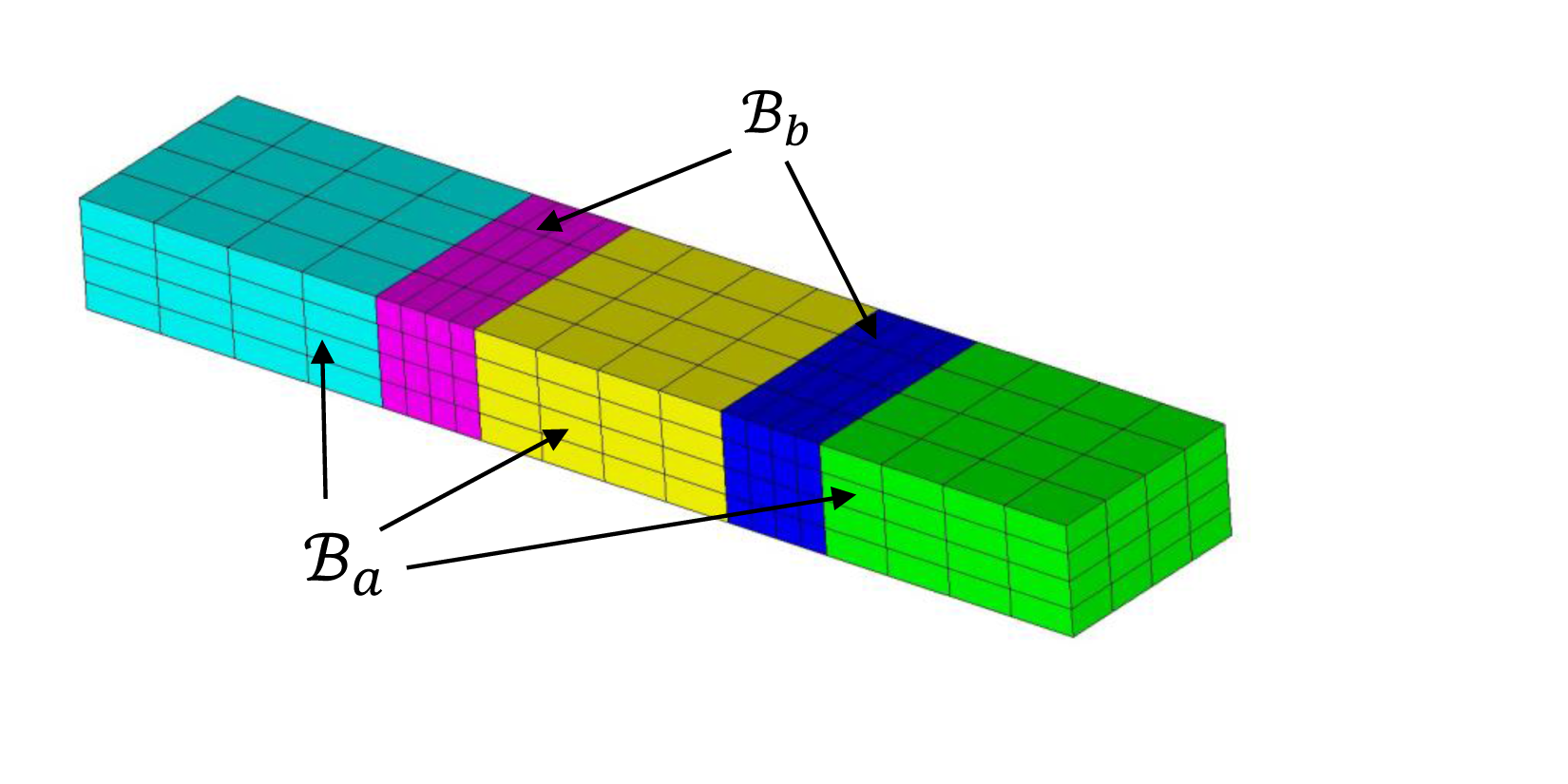
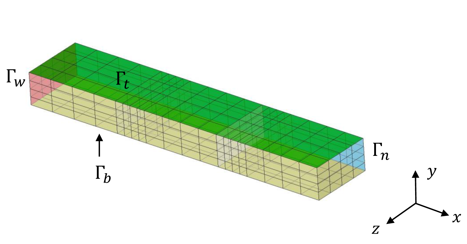
(a) Discretization of $\Omega$	(b) $\Omega$’s boundaries

Figure 1: Computational domain for the beam problem. In subfigure (a), different colors indicate different material blocks. Subfigure (b) distinguishes in color the different boundaries on which boundary conditions are prescribed.

In order to complete the problem definition, it is necessary to specify well-posed boundary conditions on our beam geometry $\Omega$. We prescribe boundary conditions on four of $\Omega$’s boundaries, shown in Figure 1(b) and denoted by $\Gamma_{w}$, $\Gamma_{b}$, $\Gamma_{t}$ and $\Gamma_{n}$. $\Gamma_{w}$ corresponds to $x=-0.08$ and is shown in red; $\Gamma_{b}$ corresponds to $y=-0.008$ and is shown in yellow; $\Gamma_{n}$ corresponds to $z=-0.016$ and is shown in blue; $\Gamma_{t}$ corresponds to $y=0.008$ and is shown in green. In both versions of our problem formulation (mechanical and thermo-mechanical; Sections 5.3.1 and 5.3.2, respectively), $\Gamma_{w}$ is fixed in the $x$-direction, $\Gamma_{n}$ is fixed in the $z$-direction and $\Gamma_{t}$ is fixed in the $y$-direction. Additionally, the following linearly-varying time-dependent pressure Neumann boundary condition is applied on $\Gamma_{b}$

$$P(t)=(7.2599\times 10^{4})t\mbox{ }\mbox{Pa},\hskip 14.22636ptt\geq 0,$$ (51)

where $t$ is a pseudo-time variable, described in more detail below. For the thermo-mechanical version of the beam problem (Section 5.3.2), an additional temperature boundary condition is prescribed on $\Gamma_{w}$; we defer discussion of this boundary condition until Section 5.3.2. For both variants of this problem, the mechanical and the thermo-mechanical beam, the system, initially at rest, is solved quasi-statically by performing a homotopy continuation with respect to the pseudo-time variable $t$ appearing in (51). This amounts to incrementing the applied boundary conditions (e.g., the pressure load (51)) with respect to $t$.

5.3.1 Mechanical beam

We will first investigate the purely mechanical response of the beam described above; hence, the governing PDEs are those described in Section 5.1.1. For this problem, the displacement boundary conditions represent 235 constrained dofs out of the 1575 total, leaving this problem with 1340 free dofs.

For the study performed herein, different material parameters are specified within different sets of blocks. Let block $\mathcal{B}_{a}$ denote the union of blocks 1, 2 and 4 (shown in green, yellow and cyan, respectively, in Figure 1(a)) and let block $\mathcal{B}_{b}$ denote the union of blocks 3 and 5 (shown in magenta and blue, respectively, in Figure 1(a)). In block $\mathcal{B}_{a}$, we set the Young’s modulus, Poisson’s ratio and density to the following values: $E_{a}=1.103\times 10^{11}\mbox{ }\mbox{Pa}$, $\nu_{a}=0.32$ and $\rho_{a}=7920\mbox{ }\mbox{kg}/\mbox{m}^{3}$, respectively. The values of these same parameters in block $\mathcal{B}_{b}$, denoted by $E_{b}$, $\nu_{b}$ and $\rho_{b}$, were varied for the purpose of ROM training and testing, are provided in Table 2. These values were generated by performing Latin Hypercube (LHC) sampling within the following parameter ranges: $E_{b}\in[1.27725\times 10^{11}\mbox{ }\mbox{Pa},2.12875\times 10^{11}\mbox{ }\mbox{Pa}]$, $\nu_{b}\in[0.24,0.4]$, $\rho_{b}\in[5940\mbox{ }\mbox{kg}/\mbox{m}^{3},9900\mbox{ }\mbox{kg}/\mbox{m}^{3}]$. After generating the training data by quasi-static advancement of the problem to time $T=7200\mbox{ }\mbox{s}$ with a time-step of 10 s, and building a set of LSPG POD ROMs (with and without preconditioning) for a wide range of ROM sizes $M$ (ranging from 1 to 721) from the resulting set of 3605 snapshots, the ROMs were tested in four additional regimes, corresponding to four different values of the material parameters in block $\mathcal{B}_{b}$. The values of $E_{b}$, $\nu_{b}$ and $\rho_{b}$ for each of these training cases are provided in Table 2. It is emphasized that the parameter variations in Table 2 led to nontrivial differences in the displacement field, which varied by as much as 20% between the different training and testing cases.

Table 2: Mechanical beam problem: summary of parameters specified in the material model in block $\mathcal{B}_{b}$ for the training and testing stages of the ROM process.

Regime	Case	$E_{b}(\times 10^{11})\mbox{ }[\mbox{Pa}]$	$\nu_{b}$	$\rho_{b}\mbox{ }[\mbox{kg}/\mbox{m}^{3}]$
training	1	1.38002	0.28028	9194.74
	2	2.11826	0.332646	7683.22
	3	1.82559	0.395908	6150.4
	4	1.56036	0.350415	9067.35
	5	1.68463	0.256473	7466.27
testing	1	1.50293	0.244704	6466.96
	2	1.54545	0.304329	6774.12
	3	1.47145	0.367092	8362.44
	4	1.703	0.32	7920

The main results for the mechanical beam problem are summarized in Figures 2–5. The reader can observe that the classical (unpreconditioned) LSPG solution does not appear in these plots. The LSPG solution is not included in our results summary because the unpreconditioned LSPG ROMs were not able to converge to a nonlinear solver tolerance smaller than $\mathcal{O}(1)$ for any of the basis sizes considered. Figure 2 plots the ROM global relative error $\mathcal{\epsilon}$ (calculated using (50)) as a function of the basis dimension for various preconditioned LSPG ROMs, including the projected solution increment ROM, indicated with a black dashed line. It can be seen that, in general, as the preconditioner is improved (from Jacobi, to Gauss-Seidel, to ILU), the accuracy of the resulting ROM solution is improved, approaching the ideal projected solution increment solution, as expected from the discussion in Section 3. Next, in Figure 3, we report wall times for the four ROMs evaluated for each of our testing cases. The wall times reported are averaged over four processors of a Linux workstation having 20 Intel Xeon CPU E5-2670 v2 CPUs. The reader can observe that the more sophisticated ILU preconditioner results in slightly larger wall times in general compared to the Jacobi and Gauss-Seidel preconditioners. This is due to a larger preconditioner construction time associated with the ILU preconditioner. As expected, the ideal preconditioner solution, which requires calculating the action of ${\bm{J}^{(k)}}^{-1}$ in every iteration as discussed in Section 4.4, is in general the costliest to obtain. The results in Figures 2 and 3 are combined in Figure 4, which shows a Pareto plot for the mechanical beam problem, in which the global relative error $\epsilon$ is plotted as a function of the wall time. From this plot, it is possible to identify the optimal preconditioner to use, based on one’s error and CPU-time requirements. The blue line in this plot traces points having Pareto optimality, which define the so-called Pareto front.

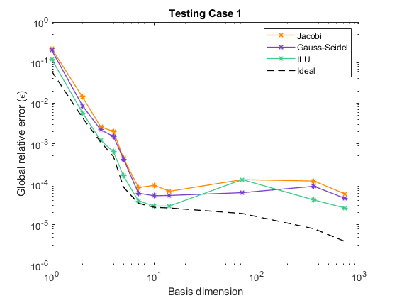
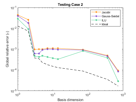
(a) Testing case 1	(b) Testing case 2
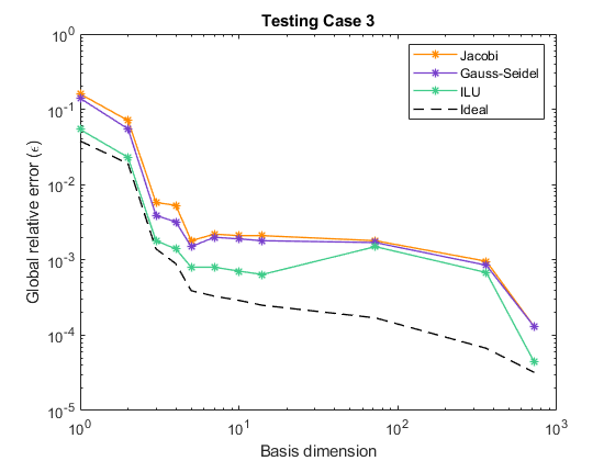
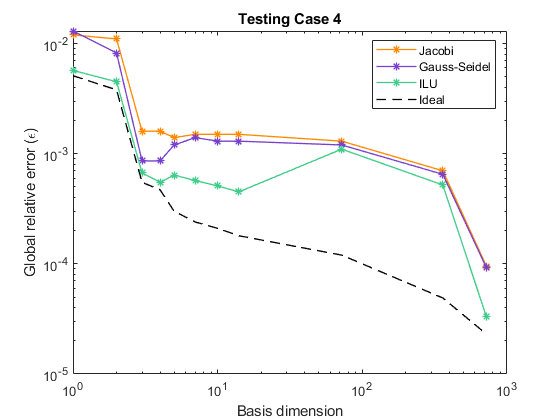
(c) Testing case 3	(d) Testing case 4

Figure 2: Mechanical beam problem: global relative errors $\mathcal{\epsilon}$ (50) for various ROMs as a function of the basis dimension for the four testing cases in Table 2.

Finally, in Figure 5, we report the average condition number of the reduced Jacobian, ${\bm{J}}_{\text{PPG}}^{(k)}$ (see (23)) over all Gauss–Newton iterations for each of the testing cases summarized in Table 2. Although the LSPG ROMs were not convergent for this problem, we include condition numbers for the LSPG ROMs in this plot. The reader can observe that, as expected, the addition of a preconditioner $\bm{M}^{(k)}$ improves the condition number of the corresponding ROM relative to the baseline LSPG ROM. For all ROMs evaluated, condition numbers grow steadily with the basis dimension $M$; however, preconditioning using the relatively simple preconditioners considered herein (the first three rows of Table 1) is able to reduce the condition number of the reduced Jacobian of the LSPG ROM by up to an order of magnitude. By design, the ideal preconditioner (equivalent to the projected solution increment) gives rise to a ROM system having a perfect condition number of one for all basis dimensions.

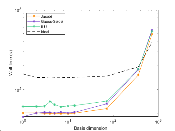
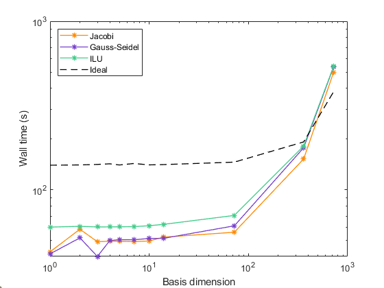
(a) Testing case 1	(b) Testing case 2
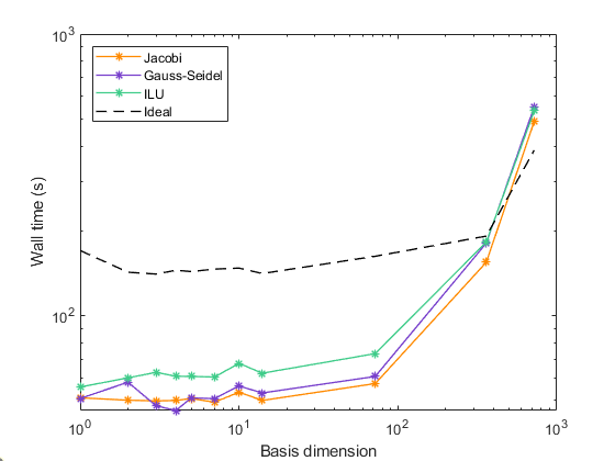
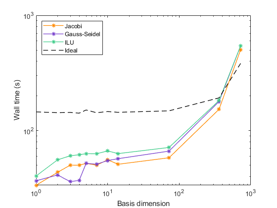
(c) Testing case 3	(d) Testing case 4

Figure 3: Mechanical beam problem: wall times (in s, averaged over 4 processors) for various ROMs as a function of the basis dimension for the four testing cases in Table 2.

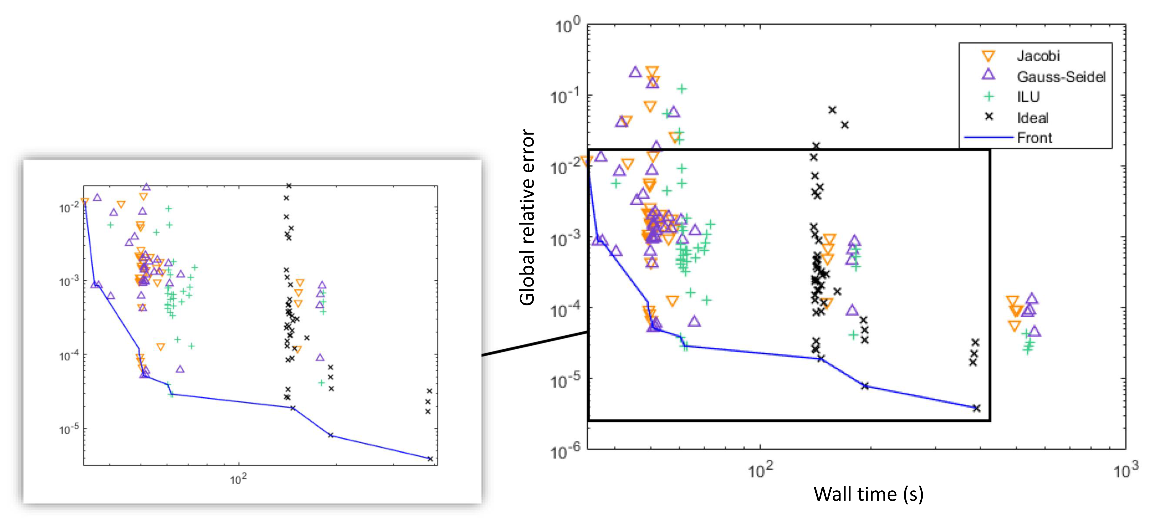
Figure 4: Mechanical beam problem: Pareto plot showing the total wall time (in s, averaged over 4 processors) versus the global relative error $\epsilon$. Results for all four testing cases in Table 2 are used to generate this figure.

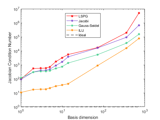
(a) Testing case 1	(b) Testing case 2
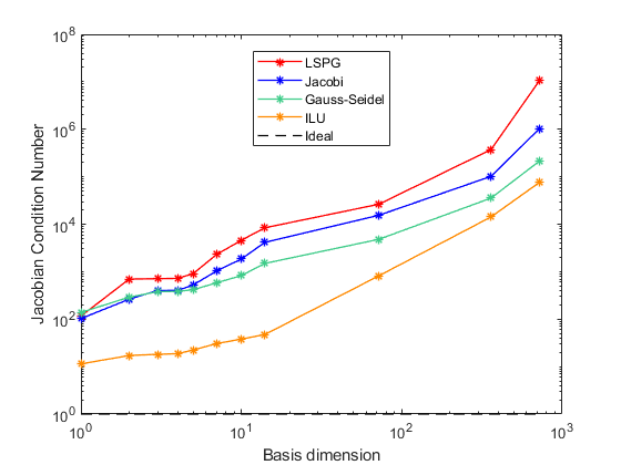
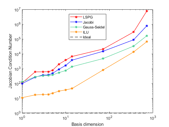
(c) Testing case 3	(d) Testing case 4

Figure 5: Mechanical beam problem: average reduced Jacobian condition number for various ROMs as a function of the basis dimension for the four testing cases in Table 2.

5.3.2 Thermo-mechanical beam

We now turn our attention to the thermo-mechanical version of the beam problem, in which the mechanical equations of Section 5.1.1 are augmented with the thermal equation in Section 5.1.2. In the current Albany implementation, the thermal and mechanical equations are coupled monolithically within the code, with the coupling occurring at the level of the material model, as described earlier in Section 5.1.2.

In addition to the displacement and pressure (51) boundary conditions described previously in Section 5.3.1, we impose a temperature Dirichlet boundary condition on $\Gamma_{w}$ in Figure 1(a). The value of the prescribed temperature varies linearly from 293 to 393 K over the course of the simulation:

$$T(t)=(100t+293)\mbox{ }\mbox{K},\hskip 14.22636ptt\geq 0.$$ (52)

As before, the variable $t$ in (52) is a pseudo-time variable which is incremented quasi-statically via homotopy continuation to emulate time-dependent behavior in a quasi-static framework. Note that the temperature boundary condition (52) is not the only one advanced in time quasi-statically; the pressure Neumann boundary condition (51) is also incremented, as discussed earlier in Section 5.3.1. As before, we use the Neohookean material model for the mechanical problem, and specify different material properties in block $\mathcal{B}_{a}$ and $\mathcal{B}_{b}$. In block $\mathcal{B}_{b}$, the mechanical properties are $E_{a}=1.103\times 10^{9}\mbox{ }\mbox{Pa}$ (Young’s modulus), $\nu_{a}=0.32$ (Poisson’s ratio) and $\rho_{a}=7.92\times 10^{-5}\mbox{ }\mbox{kg}/\mbox{m}^{3}$ (density). As discussed in Section 5.1.2, the Helmholtz free-energy density $A$ appearing in (38) is a function of the temperature $T$ in the thermo-mechanical case. This thermo-mechanical formulation requires one to specify a reference temperature. In block $\mathcal{B}_{a}$, we use a reference temperature of $T_{a,\text{ref}}=293\mbox{ }\mbox{K}$. In block $\mathcal{B}_{b}$, the mechanical properties of the Neohookean material as well as the reference temperature, denoted by $T_{b,\text{ref}}$ are varied for both the training and the testing cases, as summarized in Table 3. Additionally, we assume the material is isotropic, i.e., $\bm{K}:=k\bm{I}_{3}$ in (49), where $\bm{I}_{3}$ is the $3\times 3$ identity matrix, with thermal diffusivity $k_{a}=k_{b}=1.1870\times 10^{3}$ m²/s in both blocks. We also assume the thermal expansion coefficient (48) is the same in both blocks, taking the value $\alpha_{a}=\alpha_{b}=1\times 10^{-5}\mbox{ }\mbox{K}^{-1}$. There are no applied forces and the system is initially at rest, with an initial temperature of 293 K. For the quasi-static advancement of the system, we use a step size of 1 s and run the problem for a total of 720 steps. The displacement and temperature boundary conditions represent 260 constrained dofs out of the 2100 total dofs, leaving this problem with 1840 free dofs. As for the mechanical version of this problem, the parameter ranges in Table 3 are selected such that nontrivial variations in the solution are observed; specifically, the displacement varies by as much as 60% as the material properties are perturbed according to Table 3.

The ROM was trained with six sets of parameters in block $\mathcal{B}_{b}$, chosen using LHC sampling and summarized in Table 3. The following parameter ranges for the LHC sampling were employed: $E_{b}\in[1.27725\times 10^{9}\mbox{ }\mbox{Pa},2.12875\times 10^{9}\mbox{ }\mbox{Pa}]$, $\nu_{b}\in[0.24,0.40]$, $\rho_{b}\in[5.94\times 10^{-5}\mbox{ }\mbox{kg}/\mbox{m}^{3},9.9\times 10^{-5}\mbox{ }\mbox{kg}/\mbox{m}^{3}]$, $T_{b,\text{ref}}\in[219.75\mbox{ }\mbox{K},366.25\mbox{ }\mbox{K}]$. This training generated a total of 4318 snapshots, which were used to build various LSPG/POD ROMs (with and without preconditioning) ranging in size from 1 to 721 modes, like in the mechanical variant of this problem. These ROMs were tested in the predictive regime over four additional sets of parameters, also summarized in Table 3.

Table 3: Thermo-mechanical beam problem: summary of parameters specified in the material model in block $\mathcal{B}_{b}$ for the training and testing stages of the ROM process.

Regime	Case	$E_{b}(\times 10^{9})\mbox{ }[\mbox{Pa}]$	$\nu_{b}$	$\rho_{b}(\times 10^{-5})\mbox{ }[\mbox{kg}/\mbox{m}^{3}]$	$T_{b,\text{ref}}\mbox{ }[\mbox{K}]$
training	1	2.01313	0.285907	7.94827	273.657
	2	1.71637	0.332083	6.93965	318.406
	3	1.96881	0.3478	9.37181	301.406
	4	1.28954	0.29427	9.14636	365.378
	5	1.61326	0.262464	6.32164	223.434
	6	1.54724	0.374118	7.31561	245.778
testing	1	1.52473	0.27925	8.80694	266.674
	2	1.31153	0.345538	7.58234	333.462
	3	1.37015	0.246513	7.73303	345.942
	4	1.703	0.32	7.92	293

The main results for the thermo-mechanical beam problem are summarized in Figures 6–10. It is interesting to observe that, despite the multi-physics and multi-scale nature of this problem, the classical (unpreconditioned) LSPG ROMs, plotted in red in these figures, deliver convergent solutions for the smaller basis dimensions considered.

Figures 6 and 7 report the global relative error $\mathcal{\epsilon}$ in each of the ROM solutions, computed using (50). The reader can observe by examining this figure that, while convergence with basis refinement is observed up to a point (until $M\approx 7$ modes) for the unpreconditioned LSPG ROM, for larger basis dimensions, the error grows steadily before reaching a point where a lack of convergence is observed. The results are markedly different for the preconditioned ROMs. By introducing preconditioning, it is possible to reduce $\mathcal{\epsilon}$ by between two and six orders of magnitude, depending on the basis dimension, and there are no convergence issues, like for the unpreconditioned cases. Moreover, one can see that all the preconditioned LSPG ROMs achieve errors which are close to (less than one order of magnitude greater than) the error obtained by the projected solution increment ROM, which represents an ideal preconditioned LSPG ROM.

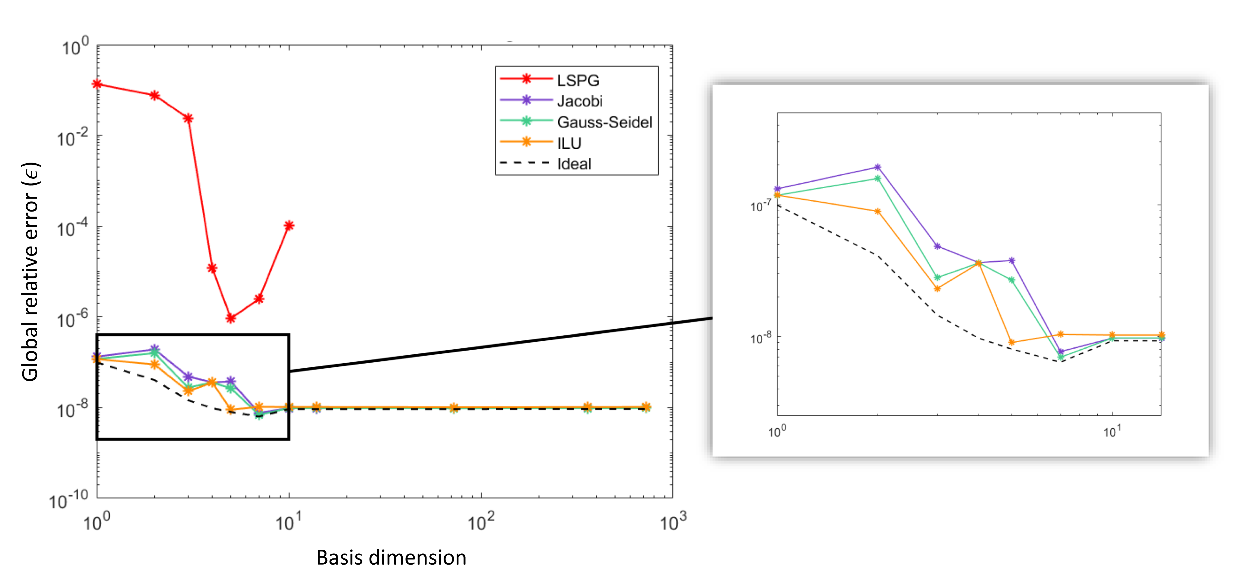
(a) Testing case 1

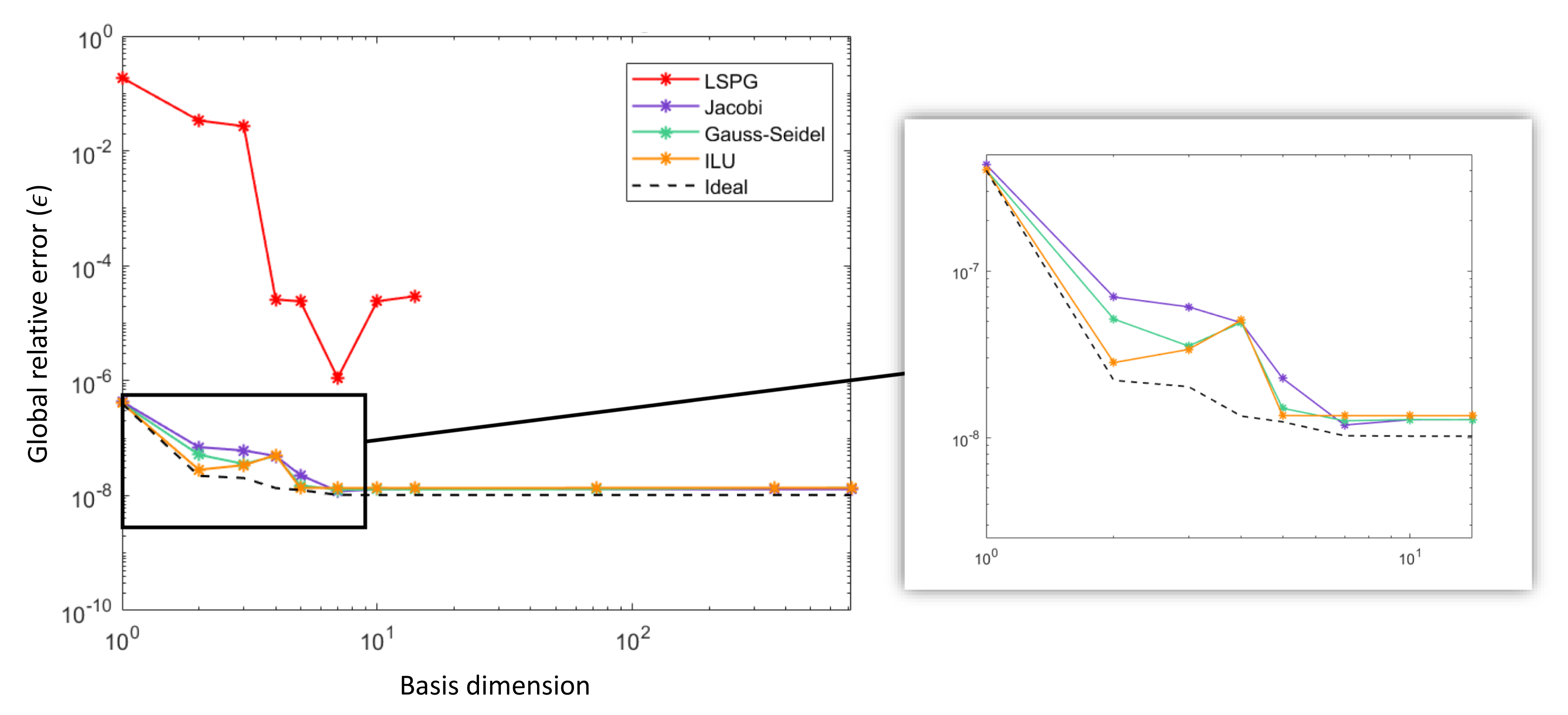
(b) Testing case 2

Figure 6: Thermo-mechanical beam problem: global relative errors $\mathcal{\epsilon}$ (50) for various ROMs as a function of the basis dimension for testing cases 1–2 in Table 3.

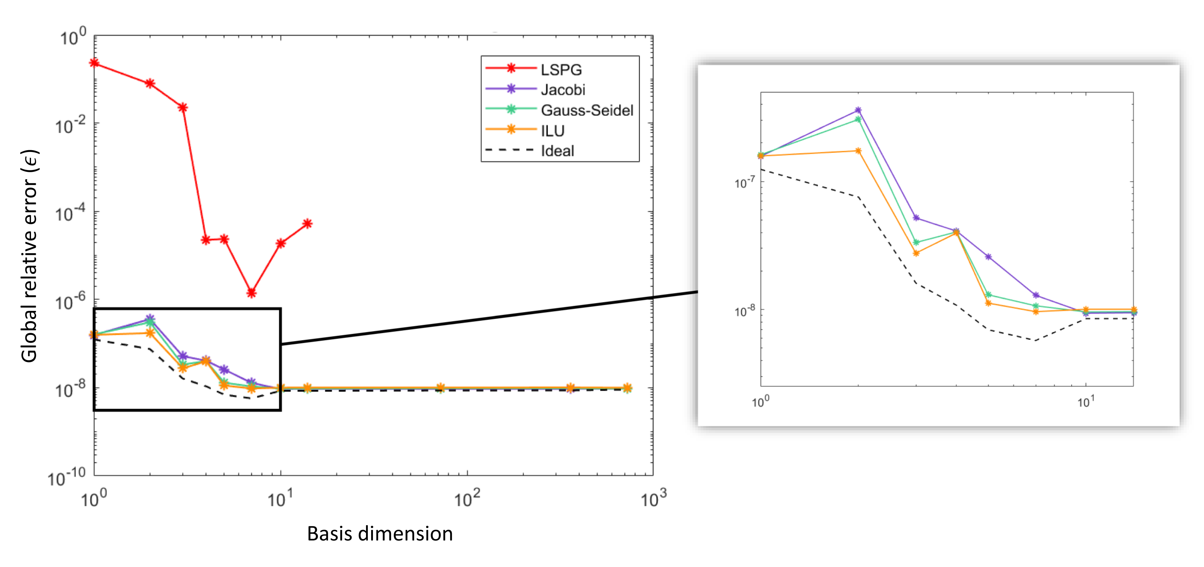
(a) Testing case 3

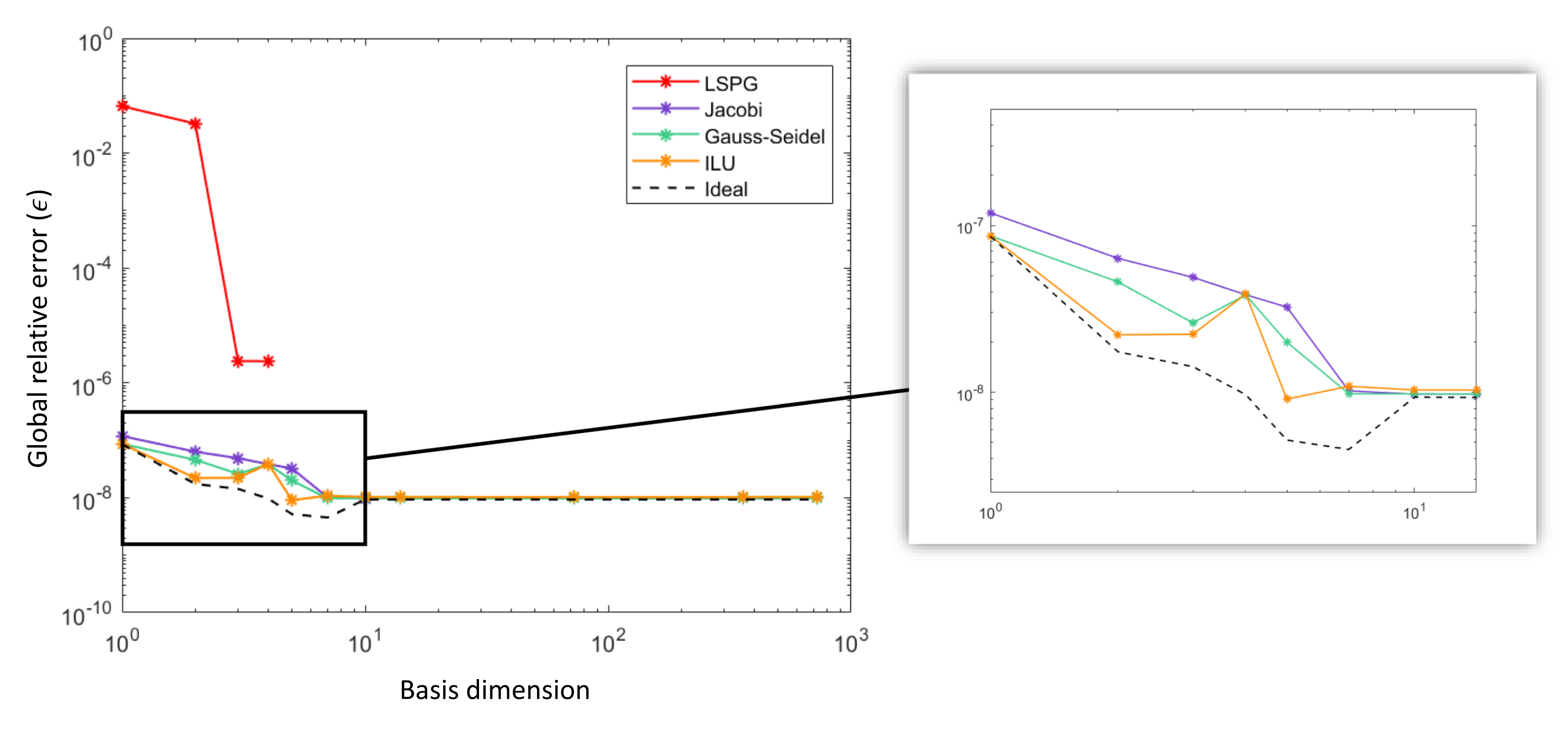
(b) Testing case 4

Figure 7: Thermo-mechanical beam problem: global relative errors $\mathcal{\epsilon}$ (50) for various ROMs as a function of the basis dimension for testing cases 3–4 in Table 3.

We next investigate the effect of preconditioning on the overall run time of the ROM problem (Figure 8). As for the mechanical version of this problem, we report wall times averaged over eight processors of a Sandia National Laboratories’ Linux cluster known as Uno, which has 201 dual-socket eight-core 2.7 GHx Intel Sandy Bridge CPUs. The reader can observe from Figure 8 that for the majority of testing cases and basis dimensions, the preconditioned LSPG ROMs considered achieve smaller wall time than the baseline (unpreconditioned) LSPG ROM. Combining these results with our earlier error results (Figures 6–7), we can confidently conclude that preconditioning is extremely advantageous for the thermo-mechanical beam problem: in general, for the same computational cost, one is able to achieve a much smaller global relative error with preconditioning. This result is confirmed in the Pareto plot shown in Figure 9. As before, the black line in Figure 8 represents the ideal preconditioned ROM. This ROM has a much higher computational cost than the other ROMs evaluated, as expected.

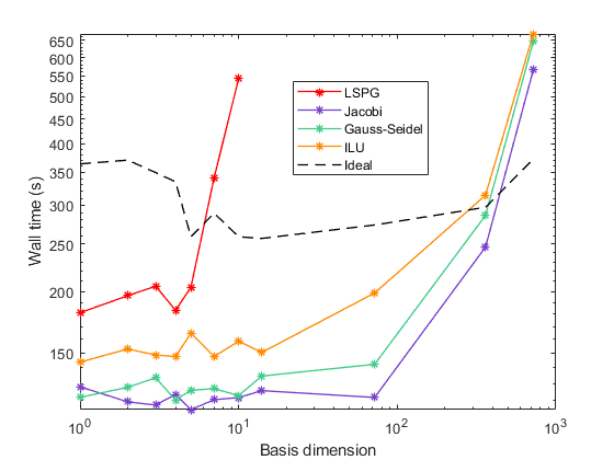
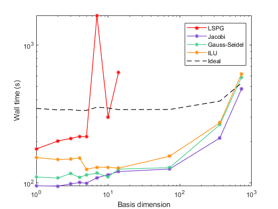
(a) Testing case 1	(b) Testing case 2
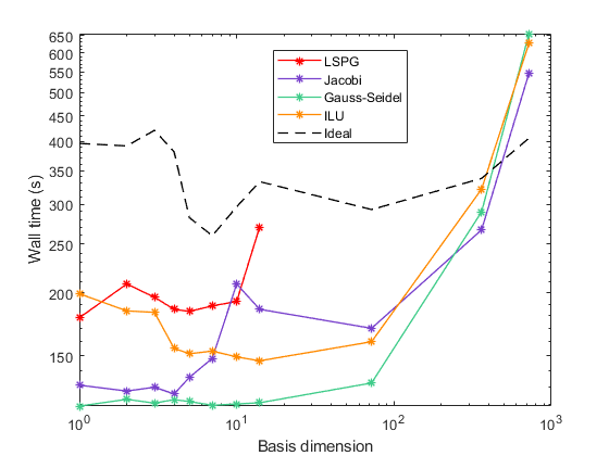
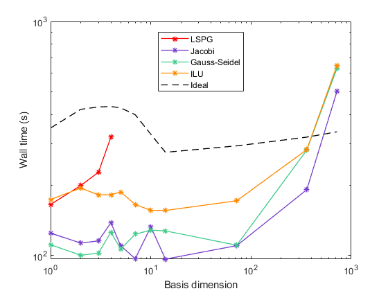
(c) Testing case 3	(d) Testing case 4

Figure 8: Thermo-mechanical beam problem: wall times (in s, averaged over 8 processors) for various ROMs as a function of the basis dimension for the four testing cases in Table 2.

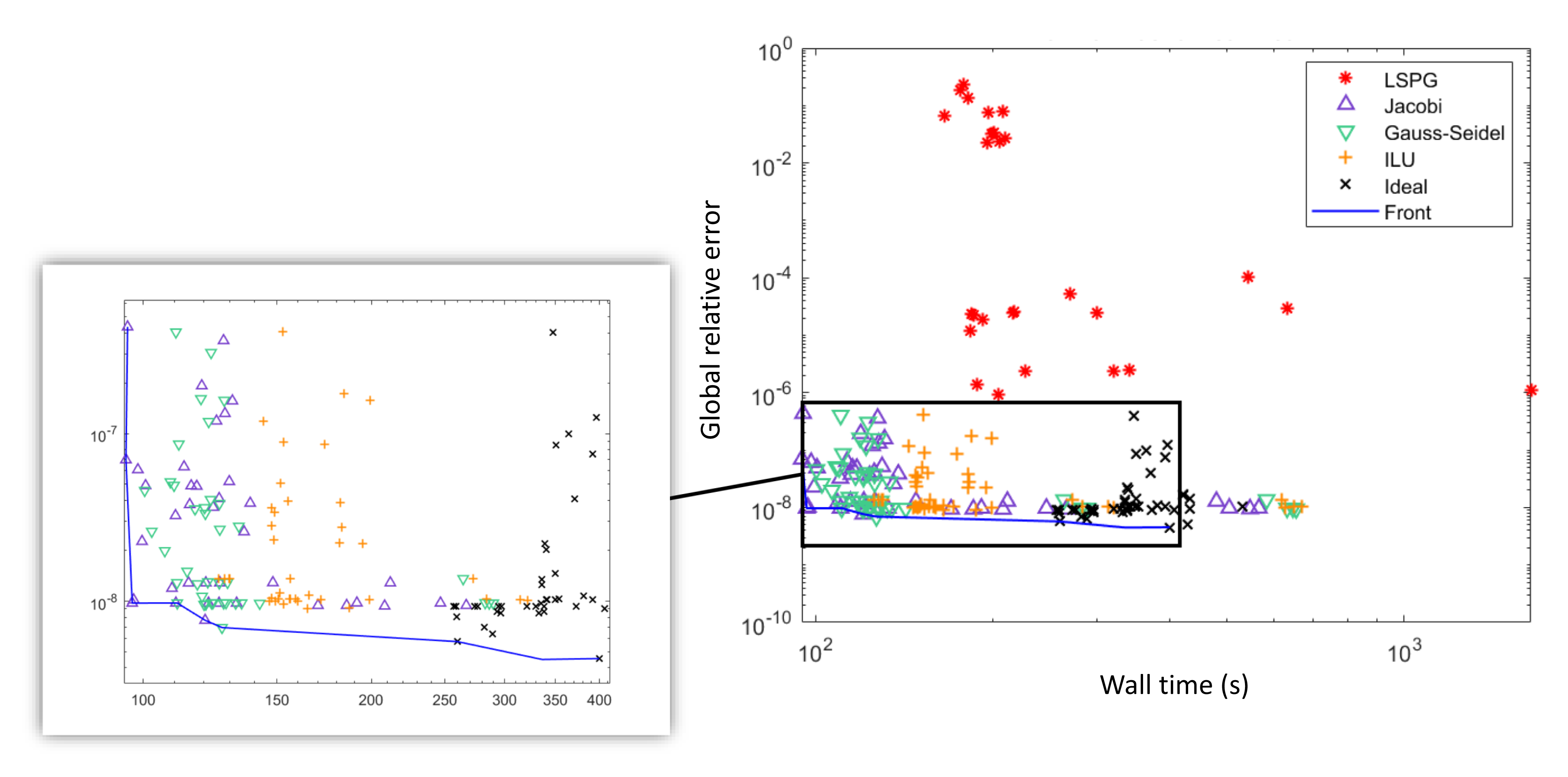
Figure 9: Thermo-mechanical beam problem: Pareto plot showing the total wall time (in s, averaged over 4 processors) versus the global relative error $\epsilon$. Results for all four testing cases in Table 3 are used to generate this figure.

Finally, in Figure 10, we report average condition numbers of the reduced Jacobians ${\bm{J}}_{\text{PPG}}^{(k)}$ (see eq. 23) encountered during the Gauss–Newton iteration process for each of the ROMs considered. The most striking observation that can be made from this figure is that the regular LSPG Jacobians are very ill-conditioned, with condition numbers ranging between $\mathcal{O}(10^{14})$ and $\mathcal{O}(10^{20})$ depending on $M$, the basis dimension. These condition numbers are between seven to ten times greater than the condition numbers for the mechanical variant of this problem (see Figure 5). The extreme ill-conditioning exhibited by the thermo-mechanical beam problem can be attributed to the extreme differences in scales between the thermal and the mechanical problems: whereas the temperature solution is $\mathcal{O}(100)$, the displacement solution varies between $\mathcal{O}(10^{-7})$ and $\mathcal{O}(10^{-5})$ during the duration of the simulation, a difference of between seven and nine orders of magnitude. Our results demonstrate that, by introducing a simple preconditioning strategy into the LSPG formulation, it is possible to bring down the reduced Jacobian condition numbers by as many as ten orders of magnitude, thereby alleviating to a large extent the scaling issue introduced by the large difference in scales between the thermal and mechanical problems (a similar result was discovered by Washabaugh in [81], but for a different application, namely computational fluid dynamics). Experience involving other solid mechanics applications within Albany [52] suggests that further improvements can be made by introducing physics-specific block preconditioners into the framework; however, a study of this sort goes beyond the scope of this work. As before, the condition number of the reduced Jacobian for the projected solution increment ROM is identically one regardless of the basis dimension.

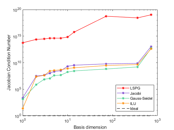
(a) Testing case 1	(b) Testing case 2
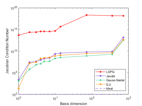
(c) Testing case 3	(d) Testing case 4

Figure 10: Thermo-mechanical beam problem: average reduced Jacobian condition number for various ROMs as a function of the basis dimension for the four testing cases in Table 3.

5.4 Thermo-mechanical pressure vessel

The last test case considered aims at studying the thermo-mechanical response of a 3D pressured cylindrical vessel shown in Figure 12(b). This problem is substantially larger and more realistic than the beam problem considered earlier in Section 5.3. Our approach herein is to model a quarter of the pressure vessel (denoted by $\Omega$), as shown in Figure 12(a), and apply appropriate symmetry boundary conditions on the relevant sides to emulate a simulation on the pressure vessel in its entirety. We discretize our domain $\Omega$ using a mesh comprised of 77,768 hexahedral elements, which give rise to 92,767 nodes. Similar to the beam problem, the domain $\Omega$ is comprised of five element blocks, depicted in green (block 1), yellow (block 2), blue (block 3), magenta (block 4) and cyan (block 5), as shown in Figure 11, so as to enable to specification of different materials and/or material properties in different parts of the domain.

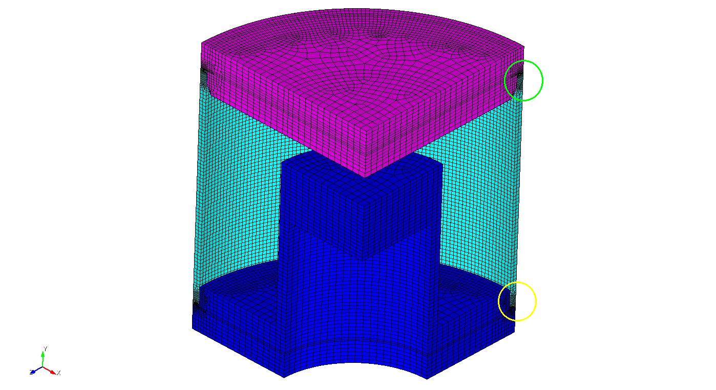
(a) All material blocks

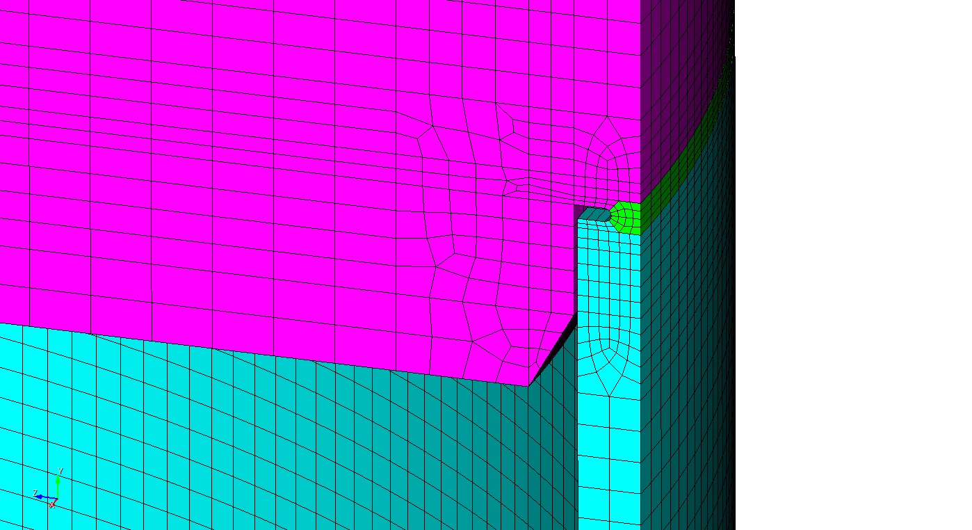
(b) Focus on block 1

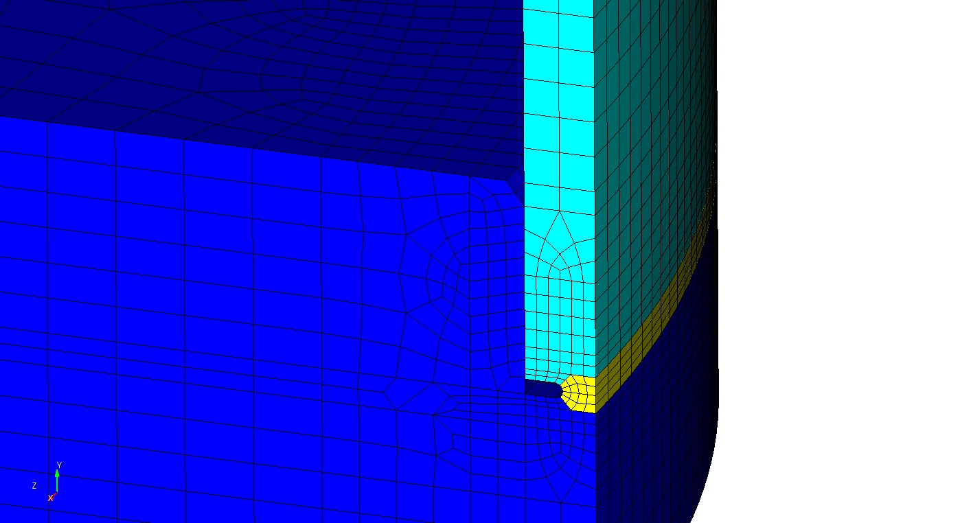
(c) Focus on block 2

Figure 11: Thermo-mechanical pressure vessel problem: computational domain. Different colors indicate different material blocks; blocks 1, 2, 3, 4 and 5 are represented in green, yellow, magenta, cyan and blue, respectively. Subfigures (b) and (c) zoom in on the regions circled in green and yellow respectively in subfigure (a), and depict the location of blocks 1 and 2, respectively.

Figure 12 depicts the boundaries on which boundary conditions are applied for the thermo-mechanical pressure vessel problem. Let $\Gamma$ denote the boundary of our computational domain $\Omega$. As shown in Figure 12(a), we decompose $\Gamma$ as $\Gamma:=\Gamma_{1}\cup\Gamma_{2}\cup\Gamma_{3}\cup\Gamma_{4}\cup\Gamma_{5}$ where $\Gamma_{i}\cap\Gamma_{j}=\emptyset$ for $i,j=1,...,5$ and $i\neq j$. In Figure 12(a), $\Gamma_{1}$ is shown in green, $\Gamma_{2}$ is shown in blue, $\Gamma_{3}$ is shown in yellow, $\Gamma_{4}$ is shown in gray and $\Gamma_{5}$ is shown in red. It is noted that $\Gamma_{5}$ consists of a single point located in the center of the top of the pressure vessel. Since we are modeling a quarter of the pressure vessel, symmetry boundary conditions are applied on the displacements on $\Gamma_{1}$, $\Gamma_{2}$ and $\Gamma_{5}$. These BCs emulate performing a simulation on the full cylindrical pressure vessel geometry (Figure 12(b)).

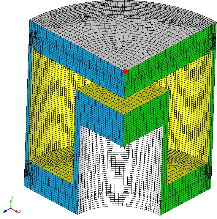
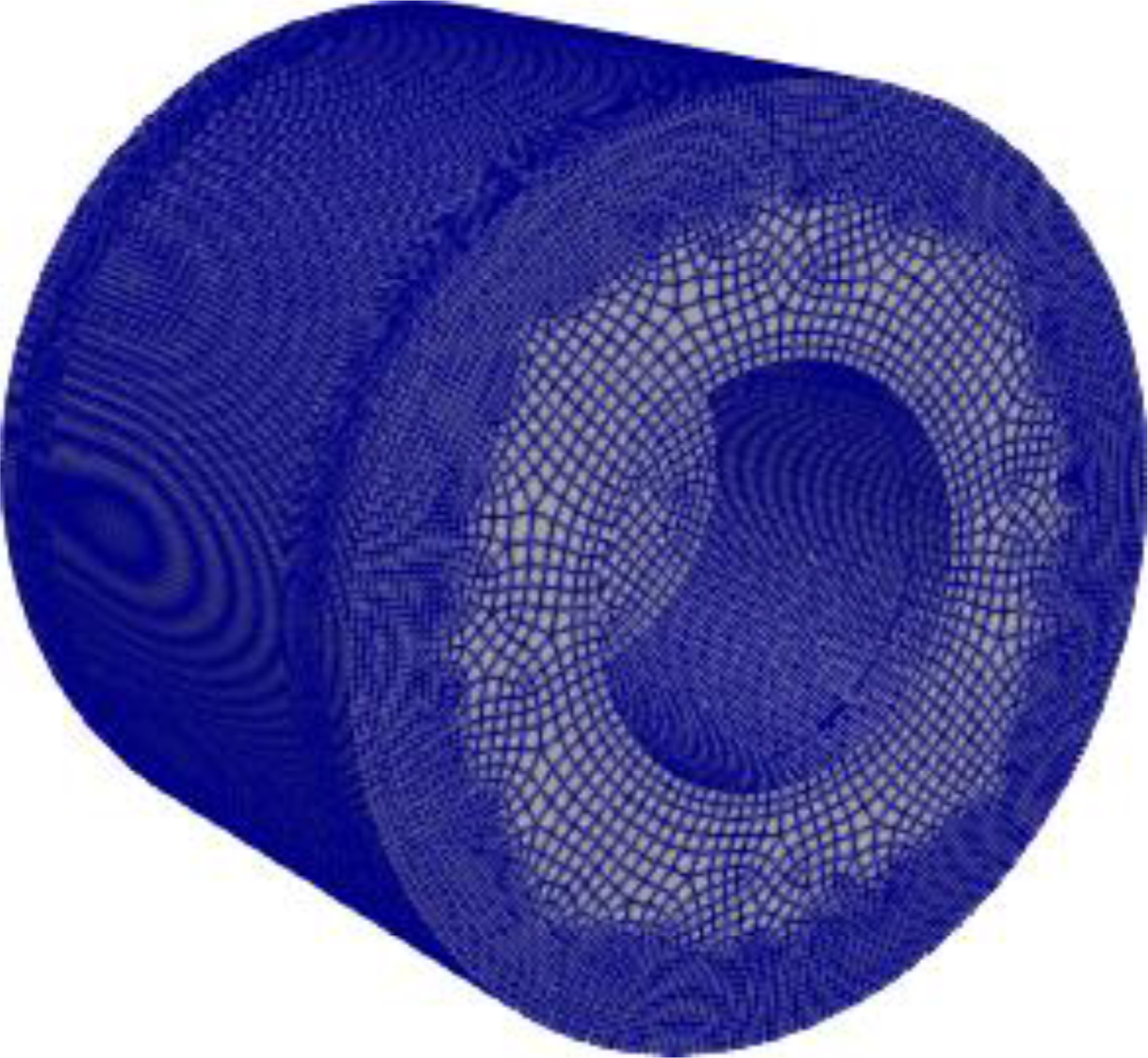
(a) Boundaries	(b) Full geometry with mesh

Figure 12: Thermo-mechanical pressure vessel problem. (a) Illustration of boundaries on which boundary conditions are applied, distinguished by different colors. $\Gamma_{1}$ is shown in green, $\Gamma_{2}$ is shown in blue, $\Gamma_{3}$ is shown in yellow, $\Gamma_{4}$ is shown in gray and $\Gamma_{5}$ is shown in red. (b) Illustration of full pressure vessel geometry following application of symmetry boundary conditions on $\Gamma_{1}$, $\Gamma_{2}$ and $\Gamma_{5}$.

In addition to the displacement boundary conditions mentioned previously, we impose the time-dependent pressure Neumann boundary condition (51) and a time-dependent temperature Dirichlet boundary condition (52) on $\Gamma_{3}$. This amounts to heating and pressurizing our vessel from the inside. The boundary conditions account for a total of 5020 constrained dofs out of the 371,068 total dofs, leaving this problem with 366,048 free dofs.

Similar to the beam problem (Section 5.3), we group together different element blocks for the purpose of specifying the material model parameters for the mechanical problem’s material model, which we take to be Neohookean. Let $\mathcal{B}_{a}$ denote the union of blocks 3 and 5 (magenta and blue, respectively, in Figure 12) and let $\mathcal{B}_{b}$ denote the the union of blocks 1, 2 and 4 (green, yellow and cyan, respectively, in Figure 12). We fix the mechanical parameters in block $\mathcal{B}_{a}$ to have the following values for the Young’s modulus, Poisson’s ratio, and density, respectively: $E_{a}=1.103\times 10^{9}\mbox{ }\mbox{Pa}$, $\nu_{a}=0.32$, and density $\rho_{a}=7.92\times 10^{-3}\mbox{ }\mbox{kg}/\mbox{m}^{3}$. The thermal equation requires us to specify a reference temperature, which is set to $T_{a,\text{ref}}=293\mbox{ }\mbox{K}$ within the thermal model. Similar to the thermo-mechanical version of the beam problem (Section 5.3.2), these analogous parameters in block $\mathcal{B}_{b}$ are varied using LHC for the purpose of training and testing our ROMs; the values of these parameters are given in in Table 4 and were sampled from the following ranges: $E_{b}\in[1.27725\times 10^{9}\mbox{ }\mbox{Pa},2.12875\times 10^{9}\mbox{ }\mbox{Pa}]$, $\nu_{b}\in[0.24,0.40]$, $\rho_{b}\in[5.94\times 10^{-3}\mbox{ }\mbox{kg}/\mbox{m}^{3},9.9\times 10^{-3}\mbox{ }\mbox{kg}/\mbox{m}^{3}]$, $T_{b,\text{ref}}\in[219.75\mbox{ }\mbox{K},366.25\mbox{ }\mbox{K}]$. The following additional parameters are also specified within the thermal model in both blocks $\mathcal{B}_{a}$ and $\mathcal{B}_{b}$. As for the thermo-mechanical beam problem (Section 5.3.2), we assume the materials are isotropic in both blocks ($\bm{K}:=k\leavevmode\nobreak\ I_{3}$), with thermal diffusivity $k_{a}=k_{b}=1.1870\times 10^{3}$ m²/s. Additionally, we assume the thermal expansion coefficient (48) is the same in both blocks, and prescribe it the value $\alpha_{a}=\alpha_{b}=1\times 10^{-5}\mbox{ }\mbox{K}^{-1}$. There are no applied forces, and the system is initially at rest with an initial temperature of $293\mbox{ }\mbox{K}$. The system is advanced using a quasi-static approach, in which the a homotopy continuation is performed with respect to the pseudo-time variable $t$ in (52). The simulation proceeds for a total of 720 steps with a step size of $1\mbox{ }\mbox{s}$.

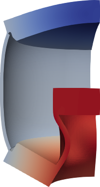
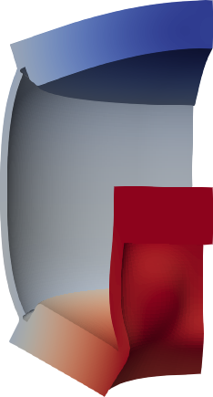
(a) Testing case 1                  (b) Testing case 2

Figure 13: Thermo-mechanical pressure vessel problem: final displacement and configuration for the two testing cases in Table 4, obtained by running Albany in FOM mode.

In this example, we trained the ROM over four sets of parameters, summarized in the top part of Table 4. Snapshots were collected every continuation step, and POD bases of various numbers of modes, from 2 to 790, were constructed using our ensemble of 2160 snapshots. Once our ROMs were constructed, they were evaluated in the predictive regime on two additional cases, summarized in the bottom part of Table 4. The final displacement FOM solutions and configurations for the two testing cases are plotted in Figure 13. The reader can observe that the solutions are noticeably different, indicating that our parameter variations led to nontrivial changes in the problem solution.

Table 4: Thermo-mechanical pressure vessel problem: summary of parameters specified in the material model in block $\mathcal{B}_{b}$ for the training and testing stages of the ROM process.

Regime	Case	$E_{b}(\times 10^{9})\mbox{ }[\mbox{Pa}]$	$\nu_{b}$	$\rho_{b}(\times 10^{-3})\mbox{ }[\mbox{kg}/\mbox{m}^{3}]$	$T_{b,\text{ref}}\mbox{ }[\mbox{K}]$
training	1	1.64424	0.39524	8.33058	311.094
	2	1.77118	0.300065	9.67843	267.396
	3	1.9893	0.32161	7.17625	223.746
	4	1.45551	0.266385	6.67746	331.116
testing	1	2.06416	0.391368	7.79804	252.102
	2	1.703	0.32	7.92	293

The main results for thermo-mechanical pressure vessel problem are summarized in Figures 14–18. Similar to the thermo-mechanical beam problem considered in Section 5.3.2, the unpreconditioned LSPG ROMs fail to converge for the two larger basis dimensions evaluated. The ideal preconditioned ROM solution is not plotted, as calculating this solution is too computationally expensive for this problem. Figure 14 plots the global relative errors $\epsilon$ (50) as a function of the basis dimension for the two testing cases of interest. The reader can observe that the unpreconditioned LSPG approach is unable to deliver a solution with a relative error smaller than $\mathcal{O}(10\%)$. In contrast, all three preconditioned LSPG ROMs produce solutions that are between four and six orders of magnitude more accurate. This result is confirmed by Figure 15, which plots the final displacement and configuration obtained using the FOM and two LSPG ROMs having 32 modes, an unpreconditioned LSPG ROM and an LSPG ROM preconditioned using the Gauss-Seidel preconditioner, for testing case 1. It can be seen that the preconditioned LSPG ROM (Figure 15(c)) is indistinguishable from the FOM (Figure 15(a)); in contrast, the unpreconditioned ROM solution (Figure 15(b)) is visibly incorrect. Turning our attention back to Figure 14, it can be seen that, by improving the preconditioner, it is possible to improve solution accuracy.

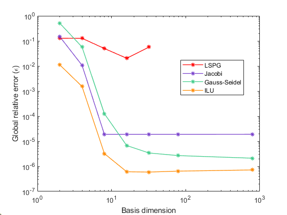
(a) Testing case 1	(b) Testing case 2

Figure 14: Thermo-mechanical pressure vessel problem: global relative errors $\mathcal{\epsilon}$ (50) for various ROMs as a function of the basis dimension for the two testing cases in Table 4.

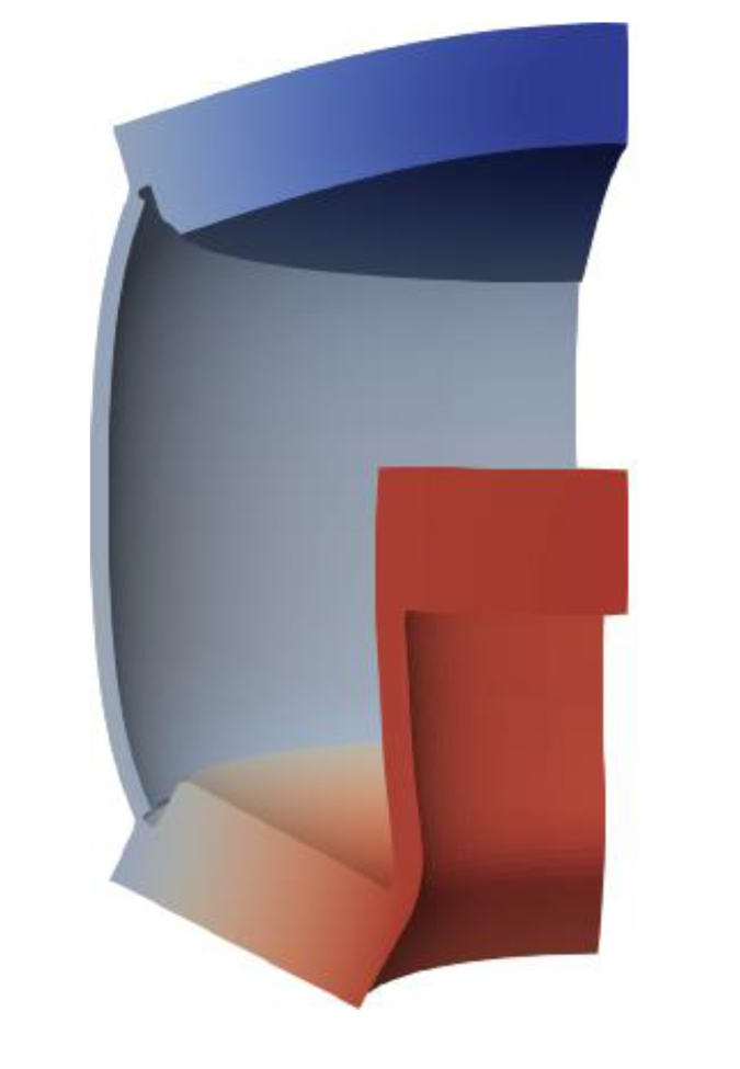
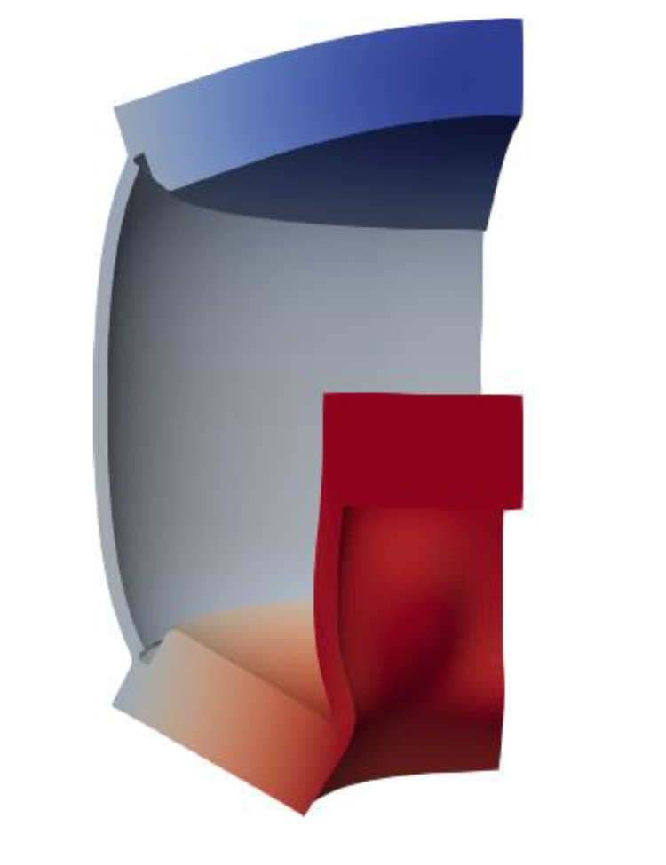
(a) FOM (b) LSPG ROM (c) Gauss-Seidel Preconditioned LSPG ROM

Figure 15: Thermo-mechanical pressure vessel problem: comparison of FOM and $M=32$ ROM solutions (final displacement and configuration) for testing case 1.

Figure 16 depicts the wall times required to run the various LSPG ROMs evaluated for each of the testing cases. Our simulations for the thermo-mechanical pressure vessel problem were performed on 64 cores (4 nodes) of the Skybridge high-capacity cluster located at Sandia National Laboratories, which contains 1848 nodes, each having 16 2.6 GHz Intel Sandy Bridge processors. It can be seen from this figure that a speedup of as large as $12\times$ is attainable through the introduction of preconditioning into the LSPG ROM formulation. Figures 14 and 16 together demonstrate that LSPG ROMs are substantially faster and more accurate than unpreconditioned LSPG ROMs. This result is reinforced by Figure 17, which depicts a Pareto plot and front for the thermo-mechanical pressure vessel problem. As before, it is possible to use this figure to determine the ideal preconditioner to use based on one’s error and CPU-time requirements.

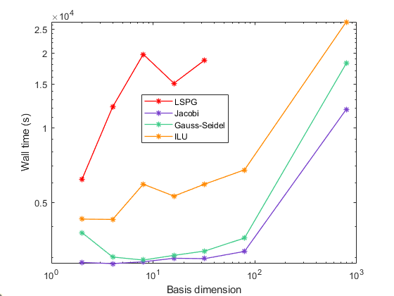
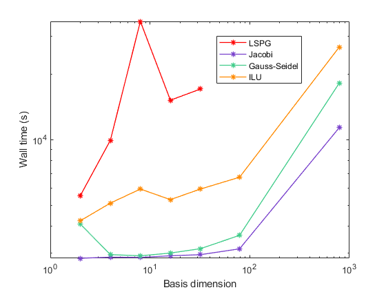
(a) Testing case 1	(b) Testing case 2

Figure 16: Thermo-mechanical pressure vessel problem: wall times (in s, averaged over 64 processors) for various ROMs as a function of the basis dimension for the two testing cases in Table 4.

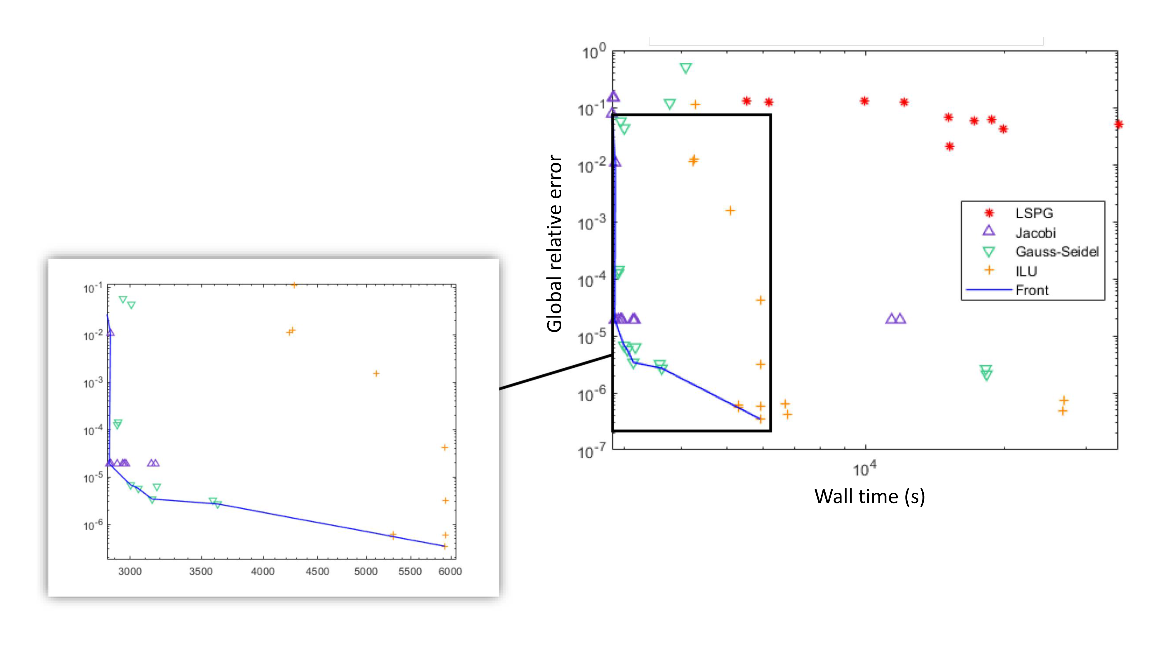
Figure 17: Thermo-mechanical pressure vessel problem: Pareto plot showing the total wall time (in s, averaged over 4 processors) versus the global relative error $\epsilon$. Results for all four testing cases in Table 3 are used to generate this figure.

Our final figure, Figure 18, plots the total number of nonlinear iterations required to attain a convergent solution for the various ROMs evaluated in this section. We present this result in lieu of the average condition number of the reduced Jacobian ${\bm{J}}_{\text{PPG}}^{(k)}$, as the thermo-mechanical pressure vessel problem is too large to calculate the latter quantity. Comparing Figure 18 with Figure 16, one can see that the wall time improvements achieved through the introduction of preconditioning are likely due to the reduction in the total number of nonlinear iterations required to achieve a convergent ROM solution: by preconditioning the LSPG formulation, one can reduce the number of nonlinear iterations by up to a factor of $12\times$. It is interesting to observe that, unlike for the classical LSPG formulation, the number of nonlinear iterations remains approximately constant regardless of the basis dimension for the preconditioned LSPG ROMs. The reduction in the number of nonlinear iterations when preconditioning is employed can be attributed to the scaling effect of the ROM preconditioner for this multi-scale and multi-physics problem.

(a) Testing case 1	(b) Testing case 2

Figure 18: Thermo-mechanical pressure vessel problem: total number of nonlinear iterations for various ROMs as a function of the basis dimension for the two testing cases in Table 4.

6 Conclusions

Projection-based model reduction can enable real-time and multi-query analyses in a variety of applications. The LSPG method to building projection-based ROMs has shown particular promise, as it can generate stable and accurate solutions for applications where standard Galerkin techniques have failed [17, 18, 75, 77, 76, 15]. Despite its superior performance over Galerkin projection, we have observed that, when run in the predictive regime, the LSPG method sometimes exhibits a lack of convergence or delivers a solution whose error surpasses the engineering tolerance required by the application. The approach is most likely to suffer from these deficiencies when applied to problems with disparate scales, such as dimensional PDEs or multi-physics problems [81, 26, 56]. This is because, when there are differences in scale between components of a PDE system, residual components corresponding to certain variables can be very large compared to the residual components corresponding to other variables, which can bias the residual minimization procedure underlying the LSPG formulation.

In this paper, we have demonstrated that the accuracy, robustness, efficiency and convergence properties of the LSPG method for projection-based model reduction can be improved substantially through the introduction of preconditioning. While this approach can reduce the condition number of the matrix problems arising in the LSPG iteration procedure, it is unlike other existing ROM preconditioning approaches (e.g., [30, 29, 69]), as the preconditioning is introduced directly into the LSPG residual minimization problem. Doing so ensures that all residual components are on approximately the same scale, even when the method is applied to multi-scale and multi-physics problems having variables of drastically different magnitudes. We demonstrated that preconditioning the LSPG method in this way is equivalent to modifying the norm in which residual minimization is performed, which can improve the residual-based stability constant bounding the method’s error. We additionally showed that, by designing a preconditioner that approximates the inverse of the Jacobian matrix, it is possible to create an LSPG ROM whose accuracy approaches the upper limit on ROM accuracy for a given reduced basis: an ideal preconditioned ROM, which is equivalent to the projection of the FOM solution increment onto the reduced basis.

We studied the efficacy of the proposed approach using one mechanical and two thermo-mechanical examples simulated using the Albany HPC multi-physics finite element code [65], into which we have implemented the POD/LSPG method to model reduction. Our test cases include a realistic simulation involving a thermo-mechanical vessel pressurized from the inside, having approximately 370,000 dofs. We developed a partitioned/“blocking vector” approach for applying ROM Dirichlet boundary conditions strongly within this code, which does not remove the constrained dofs from the global finite element system prior to performing its numerical solution. We considered three simple preconditioners, a Jacobi preconditioner, a Gauss-Seidel preconditioner, and an ILU preconditioner, implemented within the Ifpack Trilinos library, on which Albany has a dependence. Our ROMs were evaluated in the predictive regime, with prediction performed across the material parameter space. For the first test case, known as the mechanical beam problem, the classical LSPG method failed to deliver a convergent solution regardless of the basis dimension. In contrast, all three preconditioned ROMs converged robustly and efficiently, with global relative errors as small as $\mathcal{O}(0.01\%)$. While the classical LSPG method achieved convergence for the smaller basis dimensions considered in our two thermo-mechanical test cases, we demonstrated that the introduction of preconditioning can reduce the global relative error by up to six orders of magnitude and the wall time by as much as $12\times$. The wall time gains are attributed to a reduction in the reduced Jacobian condition number and a reduction in the total number of nonlinear iterations required for convergence, both achieved via the proposed preconditioning strategy. For thermo-mechanical problems, which exhibit extreme differences in scale between the displacement and temperature solutions, the introduction of even a simple preconditioner such as Jacobi reduced the reduced Jacobian condition number by as many as ten orders of magnitude.

The results discussed herein pave the way for several subsequent studies, which will be the subject of future work. First, we plan to extend our preconditioned LSPG formulation to include hyper-reduction using Lagrangian structure-preserving methods such as [33, 24, 32, 20, 23], and intend to repeat the present numerical experiments with hyper-reduction enabled. It would additionally be interesting to study: (1) the efficacy of more sophisticated preconditioners within our framework, e.g., multi-grid preconditioners that take advantage of rigid body mode information and block preconditioners for multi-physics applications, and (2) the performance of our framework with more sophisticated reduced bases, e.g., nonlinear manifold reduced bases constructed using an auto-encoder or some other type of neural network [35, 48, 46]. Lastly, we plan to investigate the viability of our approach for a larger set of applications, including problems in the field of Computational Fluid Dynamics (CFD) and problems in which the ROM is used to perform prediction in time. Our preliminary results [76, 14] suggest that preconditioning improves accuracy and efficiency in problems involving compressible cavity flows, hypersonic aerodynamics, thermal ablation and reacting hypersonic flows.

7 Acknowledgements

Support for this work was received through the U.S. Department of Energy’s (DOE) Advanced Simulation and Computing (ASC) Program at Sandia National Laboratories. The writing of this manuscript was funded in part by the third author’s Presidential Early Career Award for Scientists and Engineers (PECASE). Sandia National Laboratories is a multi-mission laboratory managed and operated by National Technology and Engineering Solutions of Sandia, LLC., a wholly owned subsidiary of Honeywell International, Inc., for the U.S. Department of Energy’s National Nuclear Security Administration under contract DE-NA0003525.

The numerical results presented herein were generated by running the Albany open-source HPC code. The version of the code that was used can be downloaded from the following URL: https://github.com/sandialabs/Albany/releases/tag/MOR_support_end. Additionally, to ensure transparency and reproducibility, we have made available the Albany input files needed to reproduce our results. These input files can be downloaded from the following github repository: https://github.com/ikalash/PrecondLSPGROMsSM.

The authors wish to thank Alejandro Mota for assisting with the formulation of the mechanical and thermo-mechanical problems described herein. The authors would also like to thank Eric Parish for providing useful feedback on the first full draft of this work, which resulted in an improved manuscript.

References

- [1] Structure-preserving model reduction for mechanical systems. Physica D: Nonlinear Phenomena, 184(1):304–318, 2003.
- [2] Anasazi: a block eigensolvers package. https://docs.trilinos.org/dev/packages/anasazi/doc/html/index.html, 2020.
- [3] MOR support end tag. https://github.com/SNLComputation/Albany/releases/tag/MOR_support_end, 2020.
- [4] NOX and LOCA: object-oriented nonlinear solver and continuation packages. https://docs.trilinos.org/dev/packages/nox/doc/html, 2020.
- [5] R. Abgrall and R. Crisovan. Model reduction using l1-norm minimization as an application to nonlinear hyperbolic problems. International Journal for Numerical Methods in Fluids, 87(12):628–651, 2018.
- [6] M. Ahmad, D. Szyld, and M. van Guzen. Preconditioned multishift BiCG for H2-optimal model reduction. SIAM J. Matrix Anal. Appl., 38:401–424, 2017.
- [7] H. Anzt, E. Chow, J. Saak, and J. Dongarra. Updating incomplete factorization preconditioners for model order reduction. Numer. Algor., 73:611–630, 2016.
- [8] P. Astrid, S. Weiland, K. Willcox, and T. Backx. Missing point estimation in models described by proper orthogonal decomposition. IEEE Transactions on Automatic Control, 53(10):2237–2250, 2008.
- [9] O. Balabanov. Randomized linear algebra for model order reduction. Ph.D. Thesis, Universitat Politecnica de Catalunya, 2019.
- [10] M. Balajewicz, I. Tezaur, and E. Dowell. Minimal subspace rotation on the stiefel manifold for stabilization and enhancement of projection-based reduced order models for the compressible navier-stokes equations. J. Comput. Phys., 321:224–241, 2016.
- [11] M.J. Balajewicz, E.H. Dowell, and B.R. Noack. Low-dimensional modelling of high-Reynolds-number shear flows incorporating constraints from the Navier-Stokes equation. J. Fluid Mech., 729:285–308, 2013.
- [12] M.F. Barone, I. Kalashnikova, M.R. Brake, and D.J. Segalman. Reduced order modeling of fluid/structure interaction. Sandia National Laboratories Report, SAND No. 2009-7189, Sandia National Laboratories, Albuquerque, NM, 2009.
- [13] M.F. Barone, I. Kalashnikova, D.J. Segalman, and H. Thornquist. Stable Galerkin reduced order models for linearized compressible flow. J. Comput. Phys., 288:1932–1946, 2009.
- [14] P. Blonigan. Personal correspondence, 2021.
- [15] K. Carlberg, M. Barone, and H. Antil. Galerkin v. least-squares Petrov–Galerkin projection in nonlinear model reduction. J. Comput. Phys., 330:693–734, 2017.
- [16] K. Carlberg, J. Cortial, D. Amsallem, M. Zahr, and C. Farhat. The GNAT nonlinear model reduction method and its application to fluid dynamics problems. AIAA Paper 2011-3112, 6th AIAA Theoretical Fluid Mechanics Conference, Honolulu, HI, June 27–30, 2011.
- [17] K. Carlberg, C. Farhat, and C. Bou-Mosleh. Efficient non-linear model reduction via a least-squares Petrov–Galerkin projection and compressive tensor approximations. International Journal for Numerical Methods in Engineering, 86(2):155–181, April 2011.
- [18] K. Carlberg, C. Farhat, J. Cortial, and D. Amsallem. The GNAT method for nonlinear model reduction: Effective implementation and application to computational fluid dynamics and turbulent flows. J. Comput. Phys., 24(2):623–647, 2013.
- [19] K. Carlberg, V. Forstall, and R. Tuminaro. Krylov-subspace recycling via the POD-augmented conjugate-gradient method. SIAM Journal on Matrix Analysis and Applications, 37(3):1304–1336, 2016.
- [20] K. Carlberg, R. Tuminaro, and P. Boggs. Efficient structure-preserving model reduction for nonlinear mechanical systems with application to structural dynamics. AIAA Paper 2012-1969, 53rd AIAA/ASME/ASCE/AHS/ASC Structures, Structural Dynamics and Materials Conference, Honolulu, HI, April 23–26, 2012.
- [21] K. Carlberg, R. Tuminaro, and P. Boggs. Preserving Lagrangian structure in nonlinear model reduction with application to structural dynamics. SIAM J. Sci. Comput., 2:B153–B184, 2015.
- [22] K. Carlberg, R. Tuminaro, and P. Boggs. Preserving lagrangian structure in nonlinear model reduction with application to structural dynamics. SIAM J. Sci. Comput, 47(2):B153–B184, 2015.
- [23] K. Carlberg, R. Tuminaro, and P. Boggs. Preserving Lagrangian structure in nonlinear model reduction with application to structural dynamics. SIAM Journal on Scientific Computing, 37(2):B153–B184, 2015.
- [24] Todd Chapman, Philip Avery, Pat Collins, and Charbel Farhat. Accelerated mesh sampling for the hyper reduction of nonlinear computational models. International Journal for Numerical Methods in Engineering, 109(12):1623–1654, 2017.
- [25] S. Chaturantabut and D.C. Sorensen. Nonlinear model reduction via discrete empirical interpolation. SIAM J. Sci. Comput., 32:2737–2764, 2010.
- [26] D. Ching, P. Blonigan, F. Rizzi, and J. Fike. Reduced order modeling of hypersonic aerodynamics with grid tailoring. AIAA SciTech Forum, January 3-7, 2022, San Diego, CA and virtual, 2022.
- [27] Y. Choi and K. Carlberg. Space-time least-squares petrov-galerkin projection for nonlinear model reduction. arXiv e-Print, (1703.04560), 2017.
- [28] Gary Collins, Krzysztof Fidkowski, and Carlos E. Cesnik. Petrov-Galerkin Projection-Based Model Reduction with an Optimized Test Space.
- [29] H. Elman and Virginia Forstall. Preconditioning techniques for reduced basis methods for parameterized elliptic partial differential equations. SIAM J. Sci. Comput., 37, 2015.
- [30] Howard C. Elman and Virginia Forstall. Numerical solution of the parameterized steady-state navier-stokes equations using empirical interpolation methods. Computer Methods in Applied Mechanics and Engineering, 317(C), 12 2016.
- [31] R. Everson and L. Sirovich. Karhunen-Loeve procedure for gappy data. J. Optical Society of America A, pages 1657–1664, 1995.
- [32] Charbel Farhat, Philip Avery, Todd Chapman, and Julien Cortial. Dimensional reduction of nonlinear finite element dynamic models with finite rotations and energy-based mesh sampling and weighting for computational efficiency. International Journal for Numerical Methods in Engineering, 98(9):625–662, 2014.
- [33] Charbel Farhat, Todd Chapman, and Philip Avery. Structure-preserving, stability, and accuracy properties of the energy-conserving sampling and weighting method for the hyper reduction of nonlinear finite element dynamic models. International Journal for Numerical Methods in Engineering, 102(5):1077–1110, 2015.
- [34] Jennifer Frederick, Alejandro Mota, Irina Tezaur, and Diana Bull. A thermo-mechanical terrestrial model of arctic coastal erosion. Journal of Computational and Applied Mathematics, 397:113533, 2021.
- [35] S. Fresca, L. Dede, and A. Manzoni. A Comprehensive Deep Learning-Based Approach to Reduced Order Modeling of Nonlinear Time-Dependent Parametrized PDEs. Journal of Scientific Computing, 87(61), 2021.
- [36] X. Gao, E. Nielsen, R. Muller, R. Young, A. Salinger, N. Bishop, M. Lilly, and M. Carroll. Quantum computer aided design simulation and optimization of semiconductor quantum dots. Journal of Applied Physics, 114:1–19, 2013.
- [37] S. Gugercin and A.C. Antoulas. A survey of model reduction by balanced truncation and some new results. Int. J. Control, 77(8):748–766, 2004.
- [38] M. Heroux. AztecOO User Guide. Sandia Report, SAND2014-3796, 2014.
- [39] M. Heroux, R. Bartlett, V. Howle, R. Hoekstra, J. Hu, T. Kolda, R. Lehoucq, K. Long, R. Pawlowski, E. Phippsand A. Salinger, H. Thornquist, R. Tuminaro, J. Willenbring, A. Williams, and K. Stanley. An overview of the trilinos project. ACM Trans. Math. Softw., 31:397–423, 2005.
- [40] Chi Hoang, Youngsoo Choi, and Kevin Carlberg. Domain-decomposition least-squares Petrov–Galerkin (DD-LSPG) nonlinear model reduction. Computer Methods in Applied Mechanics and Engineering, 384:113997, 2021.
- [41] P. Holmes, J.L. Lumley, and G. Berkooz. Turbulence, Coherent Structures, Dynamical Systems and Symmetry. Cambridge University Press, 1996.
- [42] G. Holzapfel. Nonlinear solid mechanics: a continuum approach for engineering. Wiley, 1st edition, 2000.
- [43] R. Jiang. Pressure preconditioning using proper orthogonal decomposition. M.S. Thesis, Stanford University, Stanford, CA (Advisor: H. Tchelepi), 2013.
- [44] I. Kalashnikova, S. Arunajatesan, M.F. Barone, B.G. van Bloemen Waanders, and J.A. Fike. Reduced order modeling for prediction and control of large-scale systems. Sandia National Laboratories Report, SAND No. 2014-4693. Sandia National Laboratories, Albuquerque, NM, 2014.
- [45] I. Kalashnikova and M.F. Barone. On the stability and convergence of a Galerkin reduced order model (ROM) of compressible flow with solid wall and far-field boundary treatment. J. Comput. Phys.Int. J. Numer. Meth. Engng., 83:1345–1375, 2010.
- [46] Y. Kim, D. Widemann, Y. Choi, and T. Zohdi. Efficient nonlinear manifold reduced order model. ArXiV pre-print, https://arxiv.org/pdf/2011.07727.pdf, 2021.
- [47] Sanjay Lall, Petr Krysl, and Jerrold E Marsden. Structure-preserving model reduction for mechanical systems. Physica D: Nonlinear Phenomena, 184(1):304–318, 2003. Complexity and Nonlinearity in Physical Systems – A Special Issue to Honor Alan Newell.
- [48] Kookjin Lee and Kevin T. Carlberg. Model reduction of dynamical systems on nonlinear manifolds using deep convolutional autoencoders. Journal of Computational Physics, 404:108973, 2020.
- [49] P. LeGresley. Application of proper orthogonal decomposition (pod) to design decomposition methods. Ph.D. thesis, Stanford University, 2006.
- [50] B. Moore. Principal component analysis in linear systems: Controllability, observability, and model reduction. IEEE Transactions on Automatic Control, 26(1), 1981.
- [51] A. Mota, I. Tezaur, and G. Phlipot. The Schwarz alternating method for dynamic solid mechanics. Int. J. Numer. Meth. Engng (in press), 2022.
- [52] Alejandro Mota, Irina Tezaur, and Coleman Alleman. The schwarz alternating method in solid mechanics. Computer Methods in Applied Mechanics and Engineering, 319:19 – 51, 2017.
- [53] N.C. Nguyen, A.T. Patera, and J. Peraire. A ‘best points’ interpolation method for efficient approximation of parametrized functions. Int. J. Numer. Meth. Engng., 73:521–543, 2008.
- [54] N.C. Nguyen and J. Peraire. An efficient reduced-order modeling approach for non-linear parametrized partial differential equations. Int. J. Numer. Meth. Engng., 76:27–55, 2008.
- [55] B. Noack, R. Papas, and P. Monkewitz. The need for a pressure-term representation in empirical galerkin models of incompressible shear flows. Journal of Fluid Mechanics, 523:339–365, 2005.
- [56] E. Parish and F. Rizzi. On the impact of dimensionally-consistent and physics-based inner products for pod-galerkin and least-squares model reduction of compressible flows. ArXiV pre-print, 2022.
- [57] Eric J Parish and Kevin T Carlberg. Windowed least-squares model reduction for dynamical systems. Journal of Computational Physics, 426:109939, 2021.
- [58] Damiano Pasetto, Massimiliano Ferronato, and Mario Putti. A reduced order model-based preconditioner for the efficient solution of transient diffusion equations. International Journal for Numerical Methods in Engineering, 109(8):1159–1179, 2017.
- [59] R. Pawlowski, R. Bartlett, N. Belcourt, R. Hooper, and R. Schmidt. A therory manual for multi-physics code coupling in LIME. Sandia National Laboratories Report, SAND No. 2011-2195, Sandia National Laboratories, Albuquerque, NM, 2011.
- [60] D. Rempfer and H.F. Fasel. Dynamics of three-dimensional coherent structures in a flat-plate boundary layer. Journal of Fluid Mechanics, 275:257–283, 1994.
- [61] C.W. Rowley. Model reduction for fluids using balanced proper orthogonal decomposition. Int. J. Bif. Chaos, 15(3):997–1013, 2005.
- [62] C.W. Rowley, T. Colonius, and R.M. Murray. Model reduction for compressible flows using POD and Galerkin projection. Physica D, 189:115–129, 2004.
- [63] G. Rozza. Reduced basis approximation and error bounds for potential flows in parametrized geometries. Commun. Comput. Phys., 9(1):1–48, 2011.
- [64] M. Sala and M. Heroux. Robust algebraic preconditioners with IFPACK 3.0. Technical Report SAND-0662, Sandia National Laboratories, 2005.
- [65] A. Salinger, R. Bartlett, A. Bradley, Q. Chen, I. Demeshko, X. Gao, G. Hansen, A. Mota, R. Muller, E. Nielsen, J. Ostien, R. Pawlowski, M. Perego, E. Phipps, W. Sun, and I. Tezaur. Albany: Using agile components to develop a flexible, generic multiphysics analysis code. Int. J. Multiscale Comput. Engng, 14:415–438, 2016.
- [66] A. Salinger, I. Tezaur, M. Perego, et al. Component-based application code development, part 1: The agile components strategy and albany code. Advancing X-cutting Ideas for Computational Climate Science (AXICCS) 2016, Rockville, MD, 2016.
- [67] Alexander Schein, Kevin T Carlberg, and Matthew J Zahr. Preserving general physical properties in model reduction of dynamical systems via constrained-optimization projection. International Journal for Numerical Methods in Engineering, 122(14):3368–3399, 2021.
- [68] P.J. Schmid. Dynamic mode decomposition of numerical and experimental data. Journal of Fluid Mechanics, 656:5–28, 2010.
- [69] N. P. Singh and K. Ahuja. Reusing preconditioners in projection based model order reduction algorithms. IEEE Access, 8:133233–133247, 2020.
- [70] Navneet Pratap Singh and Kapil Ahuja. Preconditioned linear solves for parametric model order reduction. International Journal of Computer Mathematics, 97(7):1484–1502, 2020.
- [71] S. Sirisup and G.E. Karniadakis. A spectral viscosity method for correcting the long-term behavior of POD models. J. Comput. Phys., 194:92–116, 2004.
- [72] L. Sirovich. Turbulence and the dynamics of coherent structures, part iii: dynamics and scaling. Q. Appl. Math., 45(3):583–590, 1987.
- [73] W. Spotz, T. Smith, I. Demeshko, and J. Fike. Aeras: A next generation global atmosphere model. Procedia Computer Science, 51:2097–2106, 2015.
- [74] W. Sun, J. Ostien, and A. Salinger. A stabilized assumed deformation gradient finite element formulation for strongly coupled poromechanical simulations at finite strain. International Journal for Numerical and Analytical Methods in Geomechanics, 37:2755–2788, 2013.
- [75] I. Tezaur, J. Fike, K. Carlberg, M. Balajewicz, M. Barone, and E. Mussoni. Model reduction for compressible cavity simulations towards uncertainty quantification of structural loading. Sandia National Laboratories Report, Sand No. 2016-9463. Sandia National Laboratories, Albuquerque, NM, 2016.
- [76] I. Tezaur, J. Fike, K. Carlberg, and M. Barone. Captive carry reduced order modeling. Sandia National Laboratories Report, Sand No. 2018-10824. Sandia National Laboratories, Albuquerque, NM, 2018.
- [77] I. Tezaur, J. Fike, K. Carlberg, M. Barone, D. Maddix, E. Mussoni, and M. Balajewicz. Advanced fluid reduced order models for compressible flow. Sandia National Laboratories Report, Sand No. 2017-10335. Sandia National Laboratories, Albuquerque, NM, 2017.
- [78] I. Tezaur, M. Perego, A. Salinger, R. Tuminaro, and S. Price. Albany/felix: A parallel, scalable and robust finite element higher-order stokes ice sheet solver built for advanced analysis. Geoscientific Model Development, 8:1–24, 2015.
- [79] P. Tiso and D. Rixen. Discrete empirical interpolation method for finite element structural dynamics. Topics in Nonlinear Dynamics, 1:203–212, 2013.
- [80] K. Veroy and A.T. Patera. Certified real-time solution of the parametrized steady incompressible Navier-Stokes equations: rigorous reduced-bases a posteriori error bounds. J. Num. Meth. Fluids, 47:773–788, 2005.
- [81] K. Washabaugh. Faster fidelity for better design. Ph.D. Thesis, Stanford University, 2016.
- [82] K. Willcox and J. Peraire. Balanced model reduction via the proper orthogonal decomposition. AIAA Journal, 40(11):2323–2330, 2002.
- [83] O. Zahm and A. Nouy. Interpolation of inverse operators for preconditioning parameter-dependent equations. SIAM J. Sci. Comput., 38:A1044–A1074, 2016.