Daniel Friedan New High Energy Theory Center and Department of Physics and Astronomy,
Rutgers, The State University of New Jersey,
Piscataway, New Jersey 08854-8019 U.S.A. and Science Institute, The University of Iceland, Reykjavik, Iceland dfriedan@gmail.com   physics.rutgers.edu/​~friedan March 22, 2022

Abstract
The dark matter in the CGF cosmology is a cosmological SU(2)-weak gauge field (the CGF). The TOV stellar structure equations are solved numerically for stars composed of this dark matter. The star mass $M$ can take any value up to a maximum $9.14\,{\times}\,10^{-6}\,\textup{M}_{\odot}$. For each value of $M$ the star radius $R$ lies between $5.23\,\text{cm}$ and $13.6\,\text{cm}$. More than one value of $R$ is possible when $M>5.09\,{\times}\,10^{-6}\,\textup{M}_{\odot}$. For those stars, a transition from larger to smaller $R$ would release gravitational energy on the order of $10^{41}\,\mathrm{J}$ in a time on the order of $10^{-10}\,\mathrm{s}$.

Contents

1. 1 Introduction
2. 2 Tolman-Oppenheimer-Volkoff equations
3. 3 CGF equation of state
4. 4 The solutions
5. 5 Abundance, clouds, seeds, binding energy
6. 6 Dark matter stars probing energies beyond the Standard Model
7. Acknowledgments

1  Introduction

The CGF cosmology is a complete theory of the Standard Model cosmological epoch, from the electroweak transition onward [1, 2]. The theory has no free parameters and assumes no physical laws beyond the Standard Model and General Relativity. All of cosmology is given by the time evolution of a uniquely determined highly symmetric semi-classical initial state in the period leading up to the electroweak transition. The CGF universe in the leading order, classical approximation contains only dark matter, no ordinary matter. The dark matter is a cosmological SU(2)-weak gauge field (the CGF). The relatively small amount of ordinary matter in the universe is a next to leading order correction to the dark matter universe from the small fluctuations of the Standard Model fields around the classical CGF. The CGF behaves effectively as a perfect fluid. Its equation of state was derived in [2] in the leading order, classical approximation. Initial fluctuations of the CGF presumably collapsed gravitationally to form self-gravitating objects. Here, the Tolman-Oppenheimer-Volkoff stellar structure equations for stars composed of CGF dark matter are solved numerically. The results are presented and some features are noted. The numerical calculations are done in SageMath [3] using the mpmath arbitrary-precision floating-point arithmetic library [4]. The Sagemath notebooks along with printouts of the notebooks are provided in the Supplemental Materials [5].

2  Tolman-Oppenheimer-Volkoff equations

The scale of the CGF fluid is set by the density (in $c=1$ units)

$$\rho_{b}=\frac{m_{\scriptscriptstyle\mathrm{Higgs}}^{4}}{\hbar^{3}}=5.68\,{\times}\,10^{28}\,{\mathrm{kg}}/{\mathrm{m}^{3}}$$ (2.1)

which is $10^{11}$ times larger than the density of a neutron star. $m_{\scriptscriptstyle\mathrm{Higgs}}$ is the mass of the Higgs boson. The associated gravitational distance and mass scales are

$$r_{b} =(4\pi G\rho_{b})^{-1/2}=1.45\,{\times}\,10^{-10}\,\text{\footnotesize s}=4.34\,\text{cm}$$ (2.2)

$$m_{b} =G^{-1}r_{b}=5.85\,{\times}\,10^{25}\,\mathrm{kg}=2.94\,{\times}\,10^{-5}\textup{M}_{\odot}=5.26\,{\times}\,10^{42}\,\text{J}$$

The TOV stellar structure equations describe the spherically symmetric static configurations of a self-gravitating perfect fluid such as the CGF. The TOV equations in dimensionless variables are

$$\begin{gathered}\frac{d\hat{p}}{d\hat{r}}=-\frac{(\hat{\rho}+\hat{p})(\hat{m}+\hat{r}^{3}\hat{p})}{\hat{r}(\hat{r}-2\hat{m})}\qquad\frac{d\hat{m}}{d\hat{r}}=\hat{r}^{2}\hat{\rho}\hat{\qquad}\frac{d\hat{e}}{d\hat{r}}=\hat{r}^{2}\hat{\rho}\left(1-\frac{2\hat{m}}{\hat{r}}\right)^{-1/2}\\[8.61108pt] \hat{r}=\frac{r}{r_{b}}\qquad\hat{m}=\frac{m}{m_{b}}\qquad\hat{e}=\frac{E_{\mathrm{tot}}}{m_{b}}\qquad\hat{\rho}=\frac{\rho}{\rho_{b}}\qquad\hat{p}=\frac{p}{\rho_{b}}\end{gathered}$$ (2.3)

$\hat{r}$ is the radial distance, $\hat{m}(\hat{r})$ and $\hat{e}(\hat{r})$ are the mass and the total energy inside $\hat{r}$, $\hat{\rho}(\hat{r})$ and $\hat{p}(\hat{r})$ are the density and pressure at $\hat{r}$. Given an equation of state relating $\hat{p}$ and $\hat{\rho}$, the TOV equations can be integrated starting from $\hat{r}=0$ with initial condition the central density $\hat{\rho}(0)$.

3  CGF equation of state

The CGF equation of state derived in [2] is

$${\begin{array}[]{cll}\hat{\rho}\geq\hat{\rho}_{\scriptscriptstyle\mathrm{EW}}\colon&\hat{p}=\frac{1}{3}\left(\hat{\rho}-c_{b}\,\hat{\rho}_{\scriptscriptstyle\mathrm{EW}}\right)&\hat{\rho}_{\scriptscriptstyle\mathrm{EW}}=7.97\quad c_{b}=0.243\\[4.30554pt] \hat{\rho}\leq\hat{\rho}_{\scriptscriptstyle\mathrm{EW}}\colon&\hat{\rho},\,\hat{p}=\hat{\rho}_{\scriptscriptstyle\mathrm{CGF}}(k^{2}),\,\hat{p}_{\scriptscriptstyle\mathrm{CGF}}(k^{2})&0\leq k^{2}\leq\frac{1}{2}\end{array}}$$ (3.1)

At densities $\hat{\rho}\geq\hat{\rho}_{\scriptscriptstyle\mathrm{EW}}$ the CGF fluid is a simple mixture of radiation and vacuum energy. The numbers $\hat{\rho}_{\scriptscriptstyle\mathrm{EW}}$ and $c_{b}$ are algebraic expressions in the Higgs coupling constant $\lambda$ and the SU(2) gauge coupling constant $g$. For $\hat{\rho}\leq\hat{\rho}_{\scriptscriptstyle\mathrm{EW}}$ the equation of state is defined implicitly by analytic functions $\hat{\rho}_{\scriptscriptstyle\mathrm{CGF}}(k^{2})$ and $\hat{p}_{\scriptscriptstyle\mathrm{CGF}}(k^{2})$ of the parameter $k^{2}$. The precise form of the two analytic functions is not illuminating. They are algebraic expressions in $k^{2}$, $\lambda$, $g$, and the complete elliptic integrals $K(k)$ and $E(k)$. The density $\hat{\rho}_{\scriptscriptstyle\mathrm{CGF}}(k^{2})$ decreases monotonically from $\hat{\rho}_{\scriptscriptstyle\mathrm{EW}}$ to $0$ as the parameter $k^{2}$ decreases from $1/2$ to $0$. The equation of state simplifies in the limit $\hat{\rho}\rightarrow 0$ to

$$\hat{p}=\frac{c_{a}}{2}\hat{\rho}^{2}+O(\hat{\rho}^{3})\qquad c_{a}=0.992$$ (3.2)

$c_{a}$ is another algebraic expression in $\lambda$ and $g$. Figure 1 plots the equation of state.

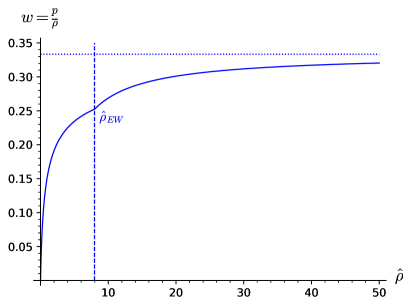
Figure 1:

4  The solutions

The TOV equations are solved numerically. The calculations are shown in the Supplemental Materials [5]. For every central density $\hat{\rho}(0)>0$ the solution reaches $\hat{\rho}=\hat{p}=0$ at a finite radial distance $\hat{r}=\hat{R}$. So each star has a well-defined radius $\hat{R}$, a well-defined mass $\hat{M}=\hat{m}(\hat{R})$, and a well-defined total energy $\hat{E}=\hat{e}(\hat{R})$.

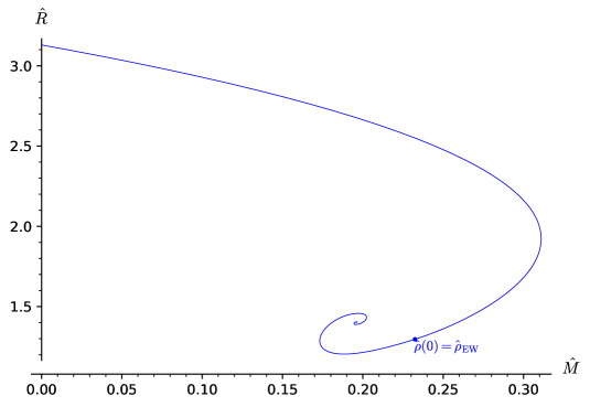
Figure 2:

Figure 2 shows the stars plotted in the $\hat{M},\hat{R}$ plane. The curve of stars is parametrized by $\hat{\rho}(0)$, starting at $\hat{\rho}(0)=0$, $M=0$. The curve spirals inward with increasing central density. The plots in Figure 3 are successive blowups showing the curve spiraling towards a fixed point. This asymptotic behavior is explained by the TOV equations for a pure radiation fluid ($w=1/3$). When the CGF central density is large, most of the evolution in $\hat{r}$ takes place with equation of state very close to that of pure radiation. The TOV equations for pure radiation are the flow equations of a vector field in the plane with a fixed point [5]. In Figure 2 the labeled point on the curve is the star with $\hat{\rho}(0)=\hat{\rho}_{\scriptscriptstyle\mathrm{EW}}$. At central densities larger than $\hat{\rho}_{\scriptscriptstyle\mathrm{EW}}$, i.e. inwards along the spiral, the star consists of a core satisfying the high density equation of state and an outer shell satisfying the low density equation of state. Within the core, the CGF holds the Higgs field at $\phi=0$. In the shell, $\phi^{\dagger}\phi$ increases from 0 at the core-shell boundary to the vacuum expectation value $v^{2}/2$ at the stellar surface. Outwards on the spiral from $\hat{\rho}_{\scriptscriptstyle\mathrm{EW}}$, at central densities $\hat{\rho}(0)\leq\hat{\rho}_{\scriptscriptstyle\mathrm{EW}}$, the stars are coreless.

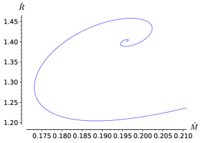
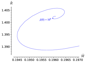
Figure 3:

5  Abundance, clouds, seeds, binding energy

The minimum radius is $\hat{R}=1.20$, $R=5.23\,\text{cm}$. The maximum radius is $\hat{R}=3.13$, $R=13.6\,\text{cm}$. The maximum star mass is $\hat{M}=0.311$, $M=1.82\,{\times}\,10^{25}\,\mathrm{kg}=9.14\,{\times}\,10^{-6}\textup{M}_{\odot}$. The abundance distribution on the star curve is calculable from first principles in the CGF cosmology, but that is beyond the scope of this paper. Microlensing observations put an upper limit $M<10^{-11}\textup{M}_{\odot}$ on compact objects as the halo dark matter [6]. Therefore most of the abundance distribution will have to be concentrated at small mass on the dark matter star curve, the limit $\hat{\rho}(0)\rightarrow 0$. The equation of state in the $\hat{\rho}(0)\rightarrow 0$ limit is $\hat{p}=\frac{1}{2}c_{a}\hat{\rho}^{2}$. The TOV equations are non-relativistic at leading order in $\hat{\rho}(0)$ and can be solved.

$$\begin{gathered}\hat{r}=c_{a}^{1/2}\theta\qquad\hat{\rho}(\hat{r})=\frac{\sin\theta}{\theta}\hat{\rho}(0)\qquad\hat{m}(\hat{r})=c_{a}^{3/2}\left(\sin\theta-\theta\cos\theta\right)\hat{\rho}(0)\\[4.30554pt] \hat{R}=\pi c_{a}^{1/2}=3.13\qquad\hat{M}=\pi c_{a}^{3/2}\hat{\rho}(0)=3.11\,\hat{\rho}(0)\\[4.30554pt] \hat{E}-\hat{M}=\frac{3\pi c_{a}^{5/2}}{4}\hat{\rho}(0)^{2}=2.31\,\hat{\rho}(0)^{2}\end{gathered}$$ (5.1)

All the small mass stars have almost exactly the same radius $\hat{R}=3.13$, $R=13.6\,\text{cm}$. We might speculate that the initial CGF fluctuations condense gravitationally to an ensemble of dark matter stars. A small fraction of the total mass is in massive dark matter stars. These become seeds for ordinary stars. The halos become populated by low mass dark matter stars — geometrically identical spheres of dark matter at low density. For mass $\hat{M}>0.173$, $M>5.09\,{\times}\,10^{-6}\textup{M}_{\odot}$ more than one value of the radius $\hat{R}$ is possible. Suppose that one of the solutions at mass $\hat{M}$ is stable and the others metastable. A star at a metastable radius might be provoked by an external influence to drop to a radius at lower gravitational energy, releasing the difference in energy. If massive dark matter stars served as seeds for formation of ordinary stars, some metastable dark matter stars might lurk in the centers of ordinary stars until provoked to release such an outburst of gravitational energy. Metastable dark matter stars might also wander without ordinary matter, emitting a burst of energy when provoked, say by a near collision. The duration of an outburst from a metastable dark matter star will be on the order of the star radius, $10^{-10}\,\text{\footnotesize s}$. To get a handle on the outburst energy, Figure 4 shows the binding energy $\hat{\mathrm{BE}}=\hat{E}-\hat{M}$ and the ratio ${\mathrm{BE}}/M=\hat{\mathrm{BE}}/\hat{M}$ (both plotted so that going downwards is energetically favored). The curve of binding energies shows that the lowest energy state for given $\hat{M}$ is the state of lowest radius. The drops in binding energy range up to about $0.05\,m_{b}=10^{41}\,\mathrm{J}$. This is about $10^{-3}$ of the energy released in a supernova. The slope of the binding energy curve shows that fusion of low mass stars with stars of almost any mass is energetically favorable. Bubbling off a small mass star is not favored. The curve of binding energy/mass shows that fission of high mass stars is not favored. Ultimately (on some time scale) all the stars will end at the bottom of the $\hat{\mathrm{BE}}/\hat{M}$ curve.

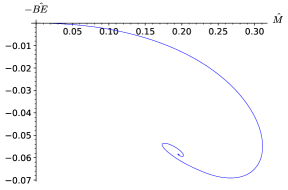
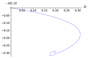
Figure 4:

6  Dark matter stars probing energies beyond the Standard Model

The energy scale at the center of the star is $\hat{\rho}(0)^{1/4}m_{\scriptscriptstyle\mathrm{Higgs}}$ so high central density stars probe energies beyond the standard model. The marked star in Figure 3 is at central density $\hat{\rho}(0)=10^{8}$. The energy scale at the star center is $10\,\mathrm{TeV}$. All the stars inward from there along the spiral curve probe energies $>10\,\mathrm{TeV}$. They would be metastable, with a rich set of possible transitions.

References

- [1] D. Friedan, “Origin of cosmological temperature,” arXiv:2005.05349 [astro-ph.CO]. May, 2020.
- [2] D. Friedan, “A theory of the dark matter,” arXiv:2203.12405 [astro-ph.CO]. March, 2022.
- [3] The Sage Developers, SageMath, the Sage Mathematics Software System (Version 9.4), 2021. https://www.sagemath.org.
- [4] F. Johansson et al., mpmath: a Python library for arbitrary-precision floating-point arithmetic (version 1.2.0), 2021. http://mpmath.org.
- [5] The accompanying Supplemental Material consists of two SageMath notebooks performing numerical calculations, along with printouts of the notebooks. The Supplemental Material is also available at physics.rutgers.edu/~friedan and cocalc.com/dfriedan/DM/SM.
- [6] H. Niikura et al., “Microlensing constraints on primordial black holes with Subaru/HSC Andromeda observations,” Nature Astron. 3 no. 6, (2019) 524–534, arXiv:1701.02151 [astro-ph.CO].