Targeted Function Balancing††thanks: I thank Chad Hazlett for advising me throughout the course of this project. I also thank Erin Hartman, Onyebuchi Arah, Mark Handcock, Avi Feller, Yixin Wang, the UCLA Causality Reading Group, and anonymous reviewers for their valuable comments and suggestions.
Abstract
This paper introduces Targeted Function Balancing (TFB), a covariate balancing weights framework for estimating the average treatment effect of a binary intervention. TFB first regresses an outcome on covariates, and then selects weights that balance functions (of the covariates) that are probabilistically near the resulting regression function. This yields balance in the regression function’s predicted values and the covariates, with the regression function’s estimated variance determining how much balance in the covariates is sufficient. Notably, TFB demonstrates that intentionally leaving imbalance in some covariates can increase efficiency without introducing bias, challenging traditions that warn against imbalance in any variable. Additionally, TFB is entirely defined by a regression function and its estimated variance, turning the problem of how best to balance the covariates into how best to model the outcome. Kernel regularized least squares and the LASSO are considered as regression estimators. With the former, TFB contributes to the literature of kernel-based weights. As for the LASSO, TFB uses the regression function’s estimated variance to prioritize balance in certain dimensions of the covariates, a feature that can be greatly exploited by choosing a sparse regression estimator. This paper also introduces a balance diagnostic, Targeted Function Imbalance, that may have useful applications.
Keywords: Augmented estimator, average treatment effect, balancing weight, causal inference, kernel, propensity score
1 Introduction
Weighting is commonly employed to estimate the causal effect of an intervention, , on an outcome of interest, . When the average treatment effect on the treated is the target estimand, and given covariates, , that make up all confounders, investigators seek weights that render the control (i.e., untreated) group more similar to the treated group on . Weights based on the probability of being treated given , or the propensity score (Rosenbaum and Rubin,, 1983), equate the distribution of in the control group to that in the treated group in expectation, and yield a weighted difference in means, , that is unbiased. But these weights require to be known or consistently estimated, which is unrealistic, and misspecifying can bring large biases (e.g., Kang and Schafer,, 2007). Another approach is to find weights that make the means of more similar between the groups, referred to here as “balancing”, or seeking “balance” in, . This can be easily extended to weights that instead, or additionally, balance a transformation of (e.g., its squares and pair-wise interactions) by replacing with, or adding to it, said transformation.
One family of balancing methods includes those that equate the means of in both groups, or balance “exactly” (e.g., Hainmueller,, 2012; Chan et al.,, 2016). However, these methods have two limitations — one of feasibility, and one of specification. On feasibility, such weights may not exist (e.g., when is of large dimension) or have high variance, resulting in a high variance . On specification, such weights only guarantee an unbiased when the conditional expectation function of given and without treatment, , is linear in . Further, these limitations compound each other — exactly balancing a high-dimensional transformation of (e.g., high-degree polynomial terms) would yield an unbiased estimator for a wider range of , but may not be possible. Thus, methods that balance “approximately”, or reduce the “imbalance” (i.e., differences in the means) to a level within some small threshold, have entered the literature in recent years (e.g, Zubizarreta,, 2015; Wang and Zubizarreta,, 2020). This approach allows weights that instead balance high-dimensional transformations of , such as basis functions from a reproducing kernel Hilbert space (e.g, Kallus,, 2020; Hirshberg et al.,, 2021; Wong and Chan,, 2018; Hazlett,, 2020; Tarr and Imai,, 2021), linear functions of which can approximate any smooth . Approximate balancing weights may thus avoid bias stemming from misspecifying . However, feasibility remains an issue — is still susceptible to bias because these weights leave imbalance in , with the average imbalance across typically increasing as does its dimension. Further, imbalance in certain elements of can be more damaging than in others, depending on their influence on . These concerns require one to proceed cautiously when exchanging with its high-dimensional transformation or prioritizing balance in select dimensions of , if at all.
But while balance in , or a transformation of it, may be sufficient for an unbiased , it is not required — in fact, all that is required is exact balance in , i.e., equality of the means of in the treated and control groups after weighting. From this perspective, seeking balance in is excessive. To illustrate, were linear in , balance in one linear function of (i.e., ) would be sufficient, but weights that balance also balance all linear functions of it — an inefficient strategy at best, and can hinder proper balance in . This perspective motivates Targeted Function Balancing (TFB), which more directly targets balance in by estimating it with , and choosing weights that balance functions near , in hopes that is among them. In short, this yields approximate balance in and , with the estimated variance of determining how much balance in is sufficient.
More specifically, TFB has several notable characteristics. First, it is an approximate balancing method, so it may exchange with a high-dimensional transformation of . This includes basis functions from a reproducing kernel Hilbert space, building on the developing literature of weights that draw on them (e.g., Kallus,, 2020; Hazlett,, 2020; Wong and Chan,, 2018; Hirshberg et al.,, 2021; Huang et al.,, 2006; Zhao,, 2019; Tarr and Imai,, 2021), by estimating with kernel regularized least squares (Hainmueller and Hazlett,, 2014). However, TFB offers a solution to feasibility concerns by narrowing the function space that the weights seek balance in, that is, from all linear functions of , to those probabilistically near per its estimated variance. Second, and relatedly, TFB primarily seeks balance in , but additionally seeks balance in to safeguard against uncertainty in , and to a degree deemed necessary by the estimated variance of . Consequently, and in contrast to traditions that advocate for good balance on every covariate (e.g., Stuart,, 2010), TFB may intentionally leave imbalance in dimensions of because they have little to no influence on , or to offset imbalances in other dimensions. This can improve feasibility and yield efficiency gains without introducing bias, as is demonstrated below. Third, the estimated variance of determines how to prioritize balance in each dimension of , a feature that can be exploited to great effect by estimating with sparsity (e.g., the LASSO). Fourth, and finally, TFB’s weights are entirely defined by the choice of regression estimator (i.e., ) and an estimator for its variance, thus turning the problem of how best to balance the covariates into how best to model the outcome.
Combining a and weights to estimate treatment effects is a well-studied research area. It is essential to the augmented (weighted) estimator, the typical form of doubly-robust estimators (e.g., Robins et al.,, 1994; Robins and Rotnitzky,, 1995; van der Laan and Rubin,, 2006; Tan,, 2010; Rotnitzky et al.,, 2012; Chernozhukov et al.,, 2018), which are consistent in a propensity score weights setting when the investigator has correctly specified or . Augmented estimators have also been applied with approximate balancing weights (e.g. Athey et al.,, 2018, Hirshberg and Wager,, 2021). In fact, TFB performs similarly to an augmented estimator in practice, so this estimator is given particular attention below. Other methods that use a in conjunction with weights include those that allow a to inform which dimensions of to prioritize balance in, or to use to estimate for propensity score weights (e.g., Shortreed and Ertefaie,, 2017; Kuang et al.,, 2017; Ning et al.,, 2020), and methods that expand on prognostic score theory from Hansen, (2008) (e.g., Leacy and Stuart,, 2014; Antonelli et al.,, 2018), which supports seeking balance in . TFB contributes to this literature by letting the estimated variance of determine how to prioritize balance in over , and in certain dimensions of over others. Additionally, this paper introduces Targeted Function Imbalance (TFI), a balance diagnostic that TFB minimizes subject to constraints on the weights’ variance. As will be elaborated on, TFI may have applications to other methods (e.g., Nikolaev et al.,, 2013; Hazlett,, 2020; Zhao,, 2019; Pirracchio and Carone,, 2018; Imai and Ratkovic,, 2014), though these will not be fully explored here.
To outline, Section 2 details notation and assumptions, and reviews reproducing kernel Hilbert spaces, which appear throughout, and Section 3 expands on the motivation for TFB. Section 4 introduces TFB (and TFI), demonstrates its merits through simulation, and proposes a closed-form estimator for TFB’s variance. Section 4 also illuminates the connection between TFB and augmented estimation. Finally, Section 5 applies TFB to the National Supported Work Demonstration (LaLonde,, 1986) data, and Section 6 concludes. Further, the main text frames TFB as an estimator of the average treatment effect on the treated, but Appendix A extends it to other estimands.
2 Background
2.1 Notation and assumptions
Notation
Let index the units of observation and let be the density function of an arbitrary random variable. Define to be an indicator variable for receiving the treatment, with the number of treated units and the number of control units. Additionally, let be the vector of treatment statuses for the sample, and let the first units make up the control group (i.e., are the indices for the control units and are the indices for the treated units). Then, let be a -dimensional vector of covariates and let be the matrix of for the sample.
| (1) |
In accordance with the potential outcomes framework (Splawa-Neyman et al.,, 1990; Rubin,, 1974), is the outcome if control and is the outcome if treated, so is observed. Implicit here is the stable unit treatment value assumption (SUTVA), that the potential outcomes for unit are not functions of the treatment statuses of other units, and that each treatment status is administered the same across the units. Further, the tuples are assumed independent and identically distributed (iid).
Of particular importance to TFB is the conditional expectation function of given , defined here as , where is the expectation over (i.e., the super-population). This allows the model:
| (2) |
where is an error term associated with potential outcome . TFB will apply the working assumption that is linear in ,
| (3) |
(3) appears restrictive because has been defined thus far as a vector of untransformed covariates. However, exchanging with, or allowing it to include, its nonlinear transformations (e.g., polynomial terms, or basis functions) makes this representation of quite general, and is the setting in which TFB largely operates.
Assumptions
This paper assumes throughout the absence of unobserved confounding in the relationship between and , otherwise known as conditional ignorability:
Assumption 1 (Conditional Ignorability)
Note that the conditional independence in Assumption 1 extends to the and (i.e.,
), as (2) implies that .
Unobserved confounders, which would violate Assumption 1, are often a concern in real-data settings, but are beyond the scope of this paper. However, sensitivity analysis to unobserved confounders is a growing field of research, particularly for estimators that use weights — see Hong et al., (2021) and Soriano et al., (2021) for examples.
Estimands and estimators
This paper primarily considers the average treatment effect on the treated (ATT),
| (4) |
However, Appendix A adapts TFB to estimate the average treatment effect, , and the average treatment effect on the controls, .
Were it observed, the sample average treatment effect on the treated (SATT),
| (5) |
would be the ideal estimator for the ATT, but the are unobserved for treated units without strong assumptions. The class of estimators studied here thus replaces in SATT with a weighted average of the for the control units, for nonnegative weights . The resulting weighted difference in means estimator has the form
| (6) |
where is an arbitrary vector of nonnegative weights for control units,
| (7) |
These weights will have mean 1 (i.e., ) in most settings considered here. However, this condition will not be required, unless otherwise noted. Section 3 discusses the conditions that must satisfy for to be unbiased.
2.2 Background on reproducing kernel Hilbert spaces
The unbiasedness of many in the literature hinges on the specification of . Thus, some, including this paper, have turned to reproducing kernel Hilbert spaces (RKHS) to characterize a large space of functions from which , or an arbitrarily close approximation, could come. This section therefore provides a brief review of the relevant points in RKHS. For a more extensive review, see Wainwright, (2019).
Background on “positive semi-definite kernel functions” is first required. A positive semi-definite kernel function, , is a symmetric function such that for all possible choices of for arbitrary , the matrix with th element equal to is positive semi-definite. Per Hazlett, (2020), it is helpful to interpret as a similarity score. For example, the primarily employed here is the Gaussian kernel, for some bandwidth parameter . This kernel’s range is 0 to 1, with only when (i.e., when and are as similar as can be), and approaches 0 as (i.e., as and diverge).
A RKHS, , is then the unique Hilbert space of functions that contains for , and has the inner product satisfying the Reproducing Property:
| (Reproducing Property) |
and norm . If , then the Reproducing Property allows the representation for and some (see Wainwright,, 2019 for proof). Thus, within the sample, any function in can be expressed as a linear function of . This representation can be quite powerful, depending on the choice of . For example, for some choices (e.g., the Gaussian kernel for any ), a function in can approximate any smooth function to an arbitrarily close degree.111 can be represented in several ways. The first is the closure of the function space , i.e., arbitrary linear combinations of for arbitrarily many . This representation illuminates why , but does not explain why, for some , functions in can approximate any smooth function. This is more easily understood from the alternate representation of where and are eigenfunctions and eigenvalues, respectively, associated with , i.e., contains linear functions of (potentially) infinite dimensional . If is flexible, then it is plausible that linear functions of it could approximate any smooth function, just like a high degree polynomial might.
Finally, extra notation is needed. Let be the matrix with th element , otherwise known as the “gram” matrix for the full sample, and let be the th row of .
| (8) |
From a similarity score perspective, holds unit ’s similarity scores to each unit in the data. Then, letting be the first columns of with rows , the may be thought of as holding unit ’s similarity scores to each control unit in the data. Accordingly, let be the last columns of with rows .
| (9) |
Finally, let be the first rows of and let the last rows of . is also the gram matrix for the control group.
| (10) |
3 Motivation for TFB
This section motivates TFB by reframing existing approaches in the weighting literature as decisions on a set of potential to seek balance in. TFB builds on this idea by letting a , an estimate of , and its estimated variance inform this decision. Section 3.1 first reviews the role that plays in the conditions the weights must satisfy for to be unbiased.
3.1 Desirable properties of the weights
Letting for a weight function ,
| (11) |
Therefore, obtaining a consistent estimate of the ATT using requires that
| (12) |
Note that the expectation on the left-hand side of (12) is over , and the expectation on the right-hand side is over , the empirical analog of which is unobserved. Deriving desirable conditions for the weights involves rewriting (12) in terms of the observed data.
Applying the law of iterative expectations, (12) becomes
| (13) |
Assumption 1 then allows one to remove the conditioning on in the inner expectations of both sides of (13), giving
| (14) |
Note that the outer expectations in (14) are now over on the left-hand-side, and on the right-hand side, the empirical analogs of which are both observed. This is seen more clearly by applying the definition of to (14), which also yields a desired condition for the weights:
| (WC) |
which will be referred to as the “weighting condition” (WC). Empirically, WC becomes
| (EWC) |
which will be referred to as the “empirical weighting condition” (EWC). In words, WC and EWC require that the means of be equated in expectation or empirically.
EWC is given particular focus below, and is thus worthwhile to discuss further. First, define the imbalance, or difference in the means, of a function of as
| (15) |
where is an arbitrary vector-valued function. How far the weights are from satisfying EWC, to be referred to as the “EWC Bias”, then has an intuitive form as the imbalance in :
| (16) |
Furthermore, the expectation of the EWC Bias is exactly the bias of . Decomposing the difference between and SATT reveals this:
| (17) |
First, SATT is unbiased for the ATT. Then, assuming that each pair of and (and thus ) are independent given and , taking the expectation of the both sides of (17) proves the result, as the terms with are then mean-zero under Assumption 1.222Many methods in the literature (e.g., Hainmueller,, 2012; Zubizarreta,, 2015; Hazlett,, 2020) choose weights that are “honest”, or entirely defined by and , which leaves all of the independent of all of the given and . As will be discussed in later sections, TFB’s weights depend on the , but can be implemented in such a way that each pair of and are independent given and . Putting these pieces together, the bias of is driven by the remaining imbalance in after weighting.
Note also that EWC (and WC) do not require complete overlap in the conditional distributions of , or
| (18) |
where is the propensity score. This is traditionally assumed in settings with propensity score weights (Rosenbaum and Rubin,, 1983). Instead, satisfying EWC with weights with mean 1 requires a much weaker overlap condition: that the average among the treated group (i.e., ) is in the range of the among the control group. This weaker overlap condition will be revisited in Section 4.6, but I thus forgo the traditional overlap assumption in (18). See also Appendix B.4 for a simulated example where TFB is effectively unbiased, but traditional overlap is violated.
3.2 Building blocks
This section reviews two families of weighting procedures in the literature: propensity score and balancing weights, the latter of which includes TFB. Within each family, focus is given to the tension between the assumptions on required for unbiasedness and the weights’ feasibility.
Propensity score weights
WC is satisfied by
| (19) |
This offers motivation for propensity score weights (Rosenbaum and Rubin,, 1983) — were to consistently estimate , then yields a consistent .333A with is also consistent, allowing . Of note is that propensity score weights satisfy WC for any . However, this comes at the price of a specification of . An incorrect specification may lead to biased (e.g., Kang and Schafer,, 2007).
Balancing weights
Satisfying WC for any is unnecessary if one has prior knowledge about . For example, if then weights that achieve exact balance in ,
| (20) |
satisfy EWC. This motivates balancing weights, which attempt to make the imbalance in small. One subfamily, originating from calibration in the survey literature (e.g., Deming and Stephan,, 1940; Deville and Särndal,, 1992), is:
| (BAL1) |
for some , and is a function that controls the variance of or distance from base weights. The constraints and are typically added.
A common approach is to require exact balance on through BAL1 by setting (e.g., Chan et al.,, 2016). A notable example is Entropy Balancing (Hainmueller,, 2012), which chooses to be the (negative) entropy, . However, exact balance exhibits two shortcomings — one of specification and one of feasibility. On specification, the resulting is only assured to be unbiased when . On feasibility, weights that achieve the exact balance in (20) may not exist (e.g., when is of large dimension) or may be extreme, resulting in a high variance . Further, these issues compound each other. One may expand to include its nonlinear transformations, finding exact balance has become infeasible.
These concerns have motivated approximate balancing weights. Within the BAL1 framework, Zubizarreta, (2015) and Wang and Zubizarreta, (2020) relax the exact balance conditions by letting . If , then presents a bias-variance tradeoff: smaller reduce the bias of the resulting , but also shrink the space of solutions for the weights, which may increase the variance of . The choice of is thus paramount to the performance of BAL1. Additionally, if , weights found by BAL1 bound the EWC Bias for the “worst-case” , or the that yields the most bias, as
| (21) |
where the first inequality in (21) becomes an equality when is in the direction of the leftover imbalance. Thus, and can be thought of as defining a space of functions from which the worst-case may come (i.e., ). Another subfamily of balancing procedures incorporates this idea directly, finding low variance weights that minimize the EWC Bias for the worst-case over some space of functions, ,
| (BAL2) |
where the constraints and are usually added. Analogous to and in BAL1, the parametrization of determines the complexity of that BAL2 aims to balance, and the size of determines how to prioritize minimizing the squared EWC Bias relative to .444For example, if , the objective function in BAL2 becomes The resulting procedure attempts to balance the worst-case linear function of , which is determined by overall balance in . determines how much balance in is prioritized over .
By removing the requirement of exact balance, approximate balancing weights can be made to appear robust to a wide range of by allowing a high-dimensional or, analogously in BAL2, a flexible . For example, some (e.g., Kallus,, 2020; Hazlett,, 2020; Wong and Chan,, 2018, Hirshberg et al.,, 2021; Zhao,, 2019; Tarr and Imai,, 2021) assume to be of a RKHS, applying the representation , and approximately balance . However, the optimal ways to choose in BAL1 or in BAL2 are unsolved problems, despite data-driven proposals available (e.g., Wang and Zubizarreta,, 2020 and Chattopadhyay et al.,, 2020 for BAL1; Kallus,, 2020 and Wong and Chan,, 2018 for BAL2). Furthermore, BAL2 estimators that use a data-driven often center it at the zero function, . Kallus, (2020), for example, uses a ball in a RKHS: for a data-driven . The worst-case function in may then be in the opposite direction of, or orthogonal to, in (i.e., ).555An orthogonal function when is perhaps illustrative. If and , a function orthogonal to would be where . Therefore, while only has any marginal effect on , balancing the worst-case linear function of would involve balancing functions that disregard any marginal effect of on . Balance on these orthogonal functions would not grant further bias reduction, were balance in to remain constant. However, requiring good balance on these functions would, at least, increase the variance of the resulting estimator, and could, at worst, distract the weights from obtaining good balance on . Further, as is allowed to be larger and more flexible, this inefficiency could be exacerbated. This concern provides the main motivation for TFB, which can be framed as BAL2 and seeks a that contains only functions close to with a user-chosen probability (e.g., 0.95).
4 Framework for TFB
4.1 A new balance diagnostic
This section introduces Targeted Function Imbalance (TFI), the balance diagnostic that TFB minimizes over the , and approximates the EWC Bias using a linear and its estimated variance.
To motivate TFI, I consider the setting where . Recall that exchanging with, or allowing it to include, its nonlinear transformations (e.g., basis functions) makes this representation of quite general. The magnitude of the EWC Bias then simplifies to
| (22) |
Then, letting be an arbitrary estimate of , (22) can be rewritten as
| (23) |
Rewriting EWC Bias as (23) may appear unhelpful, as is still unknown, but it reveals a useful approximation — consider (23) for the worst-case close to with some high level of probability (e.g., 0.95):
| (24) |
where is a set that contains 0 and for some ( will be left arbitrary here, but Section 4.4 studies it more closely). In other words, is set of small deviations such that, with probability approximately , can be recovered by subtracting one of these small deviations from . Clearly, will be defined by the distribution of .
Proceeding further thus requires a choice of . To motivate the final expression for TFI, consider the setting where is the OLS estimate using only the control units. then has an easily computed estimated variance in the sandwich variance estimator (White,, 1980),
| (25) |
where under iid data. Here, a logical is one that, after being transformed by , becomes a ball centered at the origin in which a falls with probability . This yields , where is the th quantile of a chi-squared random variable with degrees of freedom, simplifying (24) to TFI:
| (26) |
Applying TFI above with non-OLS regressions involves simply replacing with the new estimate, and with a suitable variance estimator. To preview, I primarily consider two forms of TFI. The first form applies kernel regularized least squares (Hainmueller and Hazlett,, 2014), and the second applies LASSO regression. One concern here is that the derivation above used as motivation the fact that for OLS, which may not be the case with a regularized regression, which are typically biased. However, as will be detailed in the next section, TFI allows TFB to exhibit desirable tendencies in finite samples even without guarantees that .
4.2 Choosing weights in TFB
This section introduces TFB, which finds low variance weights that minimize TFI. TFB, like Kallus, (2020), considers minimizing the conditional mean squared error of as an estimate of the SATT,
| (27) |
where the constant does not depend on the weights. Define TFB then as
| (TFB) |
where the objective function in the above approximates the EWC Bias in (27) with TFI, and substitutes the with . The objective function is convex, and MOSEK (through the Rmosek package in R) was used to solve this problem in all demonstrations here.
A key consequence of this is that TFB’s weights are not “honest”, or entirely defined by and , most notably because TFI is a function of the through (and ). This is in contrast with many seminal methods in the weighting literature (e.g., Hainmueller,, 2012; Imai and Ratkovic,, 2014; Zubizarreta,, 2015). However, dissecting TFB’s objective function is illustrative for envisioning its strengths, which all stem from consulting the outcomes. The term penalizes imbalance in , which equals the EWC Bias if . However, even if , it is unlikely that , so the term penalizes imbalance in , with the estimated variance of each determining how to prioritize balance in the .666Note that the coefficients’ covariance also plays a role, adding penalties and rewards for the signs of the leftover imbalances. To illustrate, let be two-dimensional. Then, Therefore, if , then the imbalances in the dimensions of are penalized more if they are of the same sign, and less if they are of the opposite sign. If , then imbalances are penalized more if they are of the opposite sign, and less if they are of the same sign. This yields two desirable properties. First, TFB balances to safeguard against uncertainty in and only to a degree deemed necessary by its estimated variance. Section 4.3 also demonstrates that this, while simultaneously seeking balance in , can yield intentional imbalance in certain dimensions of that offsets imbalance in others, granting efficiency gains without inviting bias. Second, the estimated variance of each determines a hierarchy in balancing the , meaning TFB incorporates variable selection. Section 4.3 shows how estimating with sparsity (e.g., the LASSO) can exploit this. Finally, controls the resulting estimator’s variance.
These qualities are not all unique to TFB. Prognostic score theory, developed by Hansen, (2008), also supports seeking balance in , inspiring some to incorporate in propensity score matching schemes (e.g., Leacy and Stuart,, 2014; Antonelli et al.,, 2018). Both Kuang et al., (2017) and Ning et al., (2020) emphasize balance in , and, along with Shortreed and Ertefaie, (2017), develop methods that use to inform variable selection, either in which dimensions of to prioritize balance in, or which dimensions to use to estimate for propensity score weights. TFB’s contribution to this literature is its allowing to guide how to prioritize balance in over , and in certain dimensions of over others. Additionally, BAL1 and BAL2 could integrate TFB’s properties by carefully choosing and , respectively — in fact, TFB is a special case of BAL2 where and . In real-data scenarios, investigators could apply content knowledge to tune and , potentially closing any performance gap between choosing arbitrary values and applying TFB. Nevertheless, TFB’s advantage is that it is defined by and , turning the problem of how best to balance into how best to linearly model . Lastly, the augmented (weighted) estimator is a general form of estimators (e.g., Athey et al.,, 2018; Hirshberg and Wager,, 2021) that bias-correct with a . Thorough discussion of this estimator is left to Section 4.5, but TFB’s seeking balance in leads to its performing similarly to an augmented estimator in practice.
There are two potential concerns with TFB that must be addressed. First, as with any balancing method, the performance of TFB’s resulting estimator is highly dependent on whether or not . Thus, the key risk with TFB is not choosing a that contains the non-linear transformations of the original covariates required for . Therefore, although it provided motivation for TFI, TFB is not recommended when is low-dimensional and OLS estimates . In fact, there is reason to believe that this form of TFB could perform worse than a method that solely seeks balance in . This is because the term in TFB that penalizes imbalance in , , goes to 0 as increases quite generally, as under mild conditions (e.g., in (25)). TFB thus allows more imbalance in as grows, assuming balance in is sufficient. While this is a favorable result when is linear in , it could induce bias when is not linear in because balance in could yield better balance in functions of that do contribute to . TFB is thus recommended when is high-dimensional, either to start or because it is a high-dimensional transformation of a smaller set of variables, and a regularized regression estimates . In this case, is believable, while balance in every dimension is likely infeasible. But TFB will use and its estimated variance to strategically leave imbalance in a way that ideally yields a highly efficient estimator.
This recommendation leads to the second potential concern — part of the motivation when deriving TFI in Section 4.1 was that , but this is not guaranteed with regularized regressions, which are typically biased. Further, even if the chosen regression estimator is asymptotically normal, choosing a consistent variance estimator is often non-trivial. This is a valid concern, and the consistency properties of and likely have implications for TFB’s asymptotic properties, as will be discussed in Section 4.6. However, note that the qualities of TFB discussed above follow directly from its objective function — that is, TFB will always value balance in , and use to determine how to prioritize balance in over the variance of its weights, and in certain dimensions of over others. These qualities are desirable in finite samples as long as , even without a guarantee that .
Finally, I introduce the two forms of TFB that are primarily considered below, which are listed in Table 1, and both apply regularized regressions. The first form is TFB-K, which estimates with kernel regularized least squares, setting and where
| (28) |
with chosen by cross-validation.777The krls function in R (from the KRLS package) is used to implement kernel regularized least squares, and employs leave-one-out cross validation for . Hainmueller and Hazlett, (2014) prove a suitable is
| (29) |
Hainmueller and Hazlett, (2014) show that is valid under the additional assumption that the have constant variance given . While this is unlikely, note that TFB-K does not require for standard errors, but rather uses it to determine how to prioritize balance in and versus the variance of the weights. Further, Appendix B.5 demonstrates that TFB-K can still perform well under heteroscedastic error. Therefore, although generally an inconsistent variance estimator may have implications for TFB’s asymptotic properties, I suspect that a violation to the constant variance assumption for (29) is not of major consequence.
The second form is TFB-L, which estimates with LASSO regression, and obtains by residual bootstrapping.888The glmnet package in R is used to implement the LASSO. The needed for regularization is found through cross-validation with the cv.glmnet function. When bootstrapping, I re-use the chosen from this cross-validation. Knight and Fu, (2000) and Chatterjee and Lahiri, (2010) prove the residual bootstrap is inconsistent under mild conditions for the LASSO’s asymptotic variance when one of more components of are zero. However, if the residual bootstrap were to underestimate the variance of the corresponding coefficients, in the context of TFB-L, this may help the variable selection induced by the LASSO. Further, the residual bootstrap does not keep TFB-L from performing well in later demonstrations, so I forgo alternative methods (e.g., Chatterjee and Lahiri,, 2011).
| Form of TFB | Regression Estimator () | Variance Estimator () |
|---|---|---|
| TFB-K | Kernel regularized least squares | Given in (29) |
| TFB-L | LASSO | Residual bootstrap |
4.3 Demonstrations
This section demonstrates TFB’s merits in two data generating processes (DGPs). TFB is compared to honest weighting procedures to illustrate the benefits of consulting the outcome for its weights. For simplicity, key aspects of the DGPs (e.g., sample size, and overlap) are not varied here. However, Appendices B.1 and B.2 examine TFB’s performance after varying these aspects.
DGP 1
The first demonstration compares TFB-K and the kernel-based weights of Hazlett, (2020) and Kallus, (2020), which balance . By compromising between seeking balance in through balance in , and through balance in , TFB-K strategically leaves imbalances in certain confounders that offset imbalances in others, and achieves minimal bias and high efficiency. This is despite little overlap in some confounders, and approximating them with .
Consider a DGP in which is drawn from a bivariate normal distribution around , one of four equally likely (cluster) centers that are not known by the researcher,
| (30) |
Unknown to the researcher, however, and depend on the proximity of to each center, given by :
| (31) |
Each unit’s proximity to its own center then determines the probability of treatment:
| (32) |
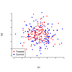
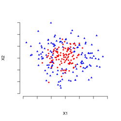
where centering the by 0.47 allows , and units closer to their center are more likely to be treated. Figure 1 shows that units with centers , , and show far more imbalance in the proximity to their center, and therefore their respective , than are units with center . Units with center will thus be referred to as those in the “easy-to-balance” cluster, and the other units will be referred to as those in the “hard-to-balance” clusters.
Finally, the outcome is linear in the ,
| (33) |
where the proximity to , captured by , is by far the most important contributor to , and there is no treatment effect (i.e., the ATT is 0). Note also that choice of results in a true of approximately 0.60.
Due to low overlap in the hard-to-balance clusters, balancing , , and would be challenging in finite samples even were they known to the researcher. However, balance in is obtainable even without balance in , , and — inducing imbalance in of the opposite sign could offset imbalance in , , and . For example, weights such that and for achieve balance in :
| (34) |
This involves reversing the sign of the original imbalance in , which is positive (see Figure 2(b)). However, due to high overlap in the easy-to-balance cluster, this may require lower variance weights than it would require to achieve exact balance in all the . Further, only slight imbalance in is needed due to the much larger influence of on than that of the other . Even though the are unobserved in reality and TFB-K must approximate them with , TFB-K should in theory be able to discern this by consulting a . Meanwhile, estimators that neglect may increase their variance by balancing the hard-to-balance clusters and unimportant dimensions of , or be too distracted by them to properly balance .
Figure 2 confirms these hypotheses, comparing TFB-K to Kernel Balancing (KBAL; Hazlett,, 2020) and Kernel Optimal Matching (KOM; Kallus,, 2020).999KBAL exactly balances (via Entropy Balancing) an -dimensional approximation (i.e., using the first eigenvectors/eigenvalues) of the gram matrix, , choosing the that minimizes the worst-case EWC Bias. The kbal function in R (from the kbal package) is used to implement KBAL. KOM fits into the BAL2 framework where is a ball in a RKHS, and with a data-driven choice of , described in Kallus, (2020). I code KOM in R from scratch, using MOSEK (through the Rmosek package in R) to solve the BAL2 problem, and the optim function in R to find . For each method, I use the Gaussian kernel, , with standardized and I forgo a kernel-selection procedure, such as that proposed by Kallus, (2020), for simplicity. Additionally, kernel regularized least squares with the Gaussian kernel and performs well here ( and are correlated at 0.936 on average), and has been found to perform well empirically (e.g., Hainmueller and Hazlett,, 2014; Schölkopf and Smola,, 2002).
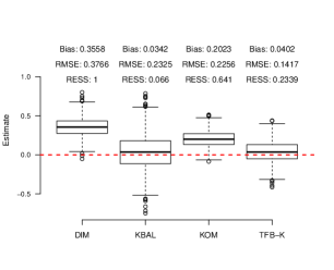
Define bias, root mean squared error (RMSE), and relative effective sample size (RESS) as
where indexes the iteration from to , and are the estimate and weight for unit , respectively, from the th iteration, and is the size of the control group in the th iteration. In Figure 2(a), TFB-K shows minimal bias, unlike KOM, and though KBAL also shows little bias, TFB-K’s RMSE is nearly two-thirds that of KBAL and KOM. Figure 2(b) reveals why this is — TFB-K leaves imbalance in of the opposite sign of the original imbalance to offset imbalance in the other . Consequently, although KBAL obtains better balance in the , its weights are higher variance than are TFB-K’s, as evidenced by TFB-K’s higher RESS (see Figure 2(a)).
TFB-K’s strategy here notably challenges traditional advice that one’s weights should attain the best balance in possible given the setting (e.g., Stuart,, 2010). However, a more universal guiding principle is that, given equal bias, a more efficient estimator is preferable. Further, TFB should in general inhibit imbalances from becoming too extreme by using the variance of to dictate how confidently it leaves imbalance. This is demonstrated in Figure 2(b) — balance is clearly a priority for TFB-K, as it successfully reduces the imbalance in each variable. Additionally, it obtains better balance in the than does KOM because, tasked with minimal overlap in the hard-to-balance clusters, KOM instead prioritizes lower variance weights, as seen in its higher RESS.101010Further discussion on KOM’s performance is warranted. Both TFB-K and KOM fit into the BAL2 framework with for some , but differ on their choices of . Presented here for KOM are the results after using the data-driven procedure suggested by Kallus, (2020) to select . However, I have found that decreasing by several factors, giving KOM more freedom to increase the variance of its weights in order to further reduce the imbalance in the , results in KOM performing on par with TFB-K in terms of bias and RMSE. Thus, TFB-K may only outperform KOM in the presented results because it happens to more effectively compromise imbalance reduction and variance in the specific DGP, rather than because it has chosen a that allows it to more effectively target balance in , which is TFB-K’s central motivation.
Finally, note that whether or not TFB-K leaves negative imbalance in at a given sample size is sensitive to (i) the for the model and (ii) the level of overlap in . Appendix B.1 explores this connection more in-depth. However, to summarize, when the is higher, TFB-K more confidently leaves imbalance in because has lower variance. Further, with more overlap in , leaving negative imbalance in is a viable strategy because it does not require outlandishly high variance weights.
DGP 2
Next, TFB can prioritize balance in the dimensions of that are most influential on by estimating with sparsity. This section demonstrates this by applying TFB-L, which estimates with LASSO regression, in a high-dimensional setting.
Consider a DGP in which contains three types of variables: (i) “confounders”, , that are related to both and ; (ii) “distractors”, , that are related to , and are difficult to balance, but are unrelated to ; and (iii) “extraneous” variables, , that are independent of both and . The outcome and the log odds of treatment are both linear in ,
| (35) | ||||
| (36) |
where the are equally imbalanced, and have varying levels of influence on . Furthermore, the ATT is 0, and allows the true to be approximately 0.50. The , the distractors (), and the extraneous variables () are then generated as
| (37) |
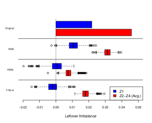
Balance in is sufficient to unbiasedly estimate the ATT. However, and , particularly which is significantly more imbalanced than is , complicate balancing the entirety of . However, TFB-L performs well by finding by LASSO regression. Figure 3 compares TFB-L with BAL1 where the are all equal.111111Specifically, BAL1 here is the method from Zubizarreta, (2015) with implied by the approx.balance function in R (from the balanceHD package) with default parameters. Further, to make the task of balancing more challenging for each method, TFB-L and BAL1 expand on , additionally (and needlessly) seeking balance in its squares and pairwise interactions, a total of 209 variables. Figure 3 also includes TFB-K to further illustrate the effect of TFB-L’s estimating with sparsity.121212As in DGP 1, TFB-K uses the Gaussian kernel with bandwidth .

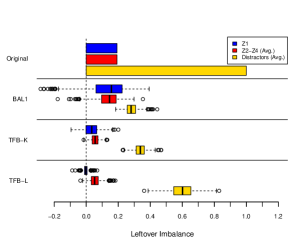
TFB-L shows minimal bias, while BAL1 is more comparable to a difference in means. TFB-L also boasts a lower RMSE than BAL1 by over a factor of two, and a higher RESS. TFB-K also performs well here, and is a marked improvement over BAL1 in both bias and RMSE, but falls short of TFB-L. Note also that TFB-L’s strong performance here persists even after varying key aspects of DGP 2 (see Appendix B.2).
As in DGP 1, the leftover imbalance in Figure 3(b) reveals why TFB-L excels. Balancing the distractors in keeps BAL1 from properly balancing and reduces its RESS. Meanwhile, TFB-L largely disregards balance in , and obtains good balance in the , particularly in , the most influential variable on . This is a byproduct of how TFB-L models — LASSO regression forces coefficients in to 0 when their respective variables are weakly correlated with , deflating their variances. Accordingly, Figure 4 shows that the distractors’, extraneous variables’, and polynomial terms’ diagonal elements in are small, illuminating why TFB-L devalues balance in those variables.
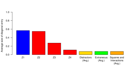
Additionally, the diagonal elements for the in increase with the size of their coefficients in the model for . Meanwhile, this variable selection does not carry over to TFB-K — it obtains balance on the distractors at almost the level of BAL1, while falling short of TFB-L’s balance in . This is because kernel regularized least squares does not estimate coefficients for with sparsity, so the diagonal entries of , given by (29), depend more on the variance of the elements of than on their contribution to . Nevertheless, TFB-K still obtains far better balance on than does BAL1, which explains its improved performance.
Discussion
First, it is important to note that in both DGPs 1 and 2, the applications of TFB either correctly specified (in DGP 2), or well-approximated with a kernel expansion (in DGP 1). However, as mentioned previously, one risk with TFB is choosing a and regression method that misspecifies or does not estimate it well. Appendix B.3 demonstrates that bias can be a consequence of this.
Second, in these demonstrations TFB achieved efficiency gains by leaving imbalance in certain variables — either to offset imbalances in other variables, or because they had little to no influence on the outcome. This presents a challenge from a diagnostics perspective, as in practice one can never know if imbalance that TFB leaves is cause for concern or if it can be safely ignored. However, note that in both DGPs 1 and 2, TFB achieved good balance on the variables that were most influential on the outcome. Thus, in practice, I suggest first confirming that TFB has obtained good balance on the variables the researcher expects to be the most influential on the outcome, determined by content knowledge, or by calculating the partial correlations between each variable and the outcome. Then, one should confirm that the variables that TFB leaves more imbalance in are the variables that one expects to be less influential. Section 5 provides an example of this on real data.
4.4 Choosing
It is now worthwhile to examine , the probability threshold in TFB. Note that influences TFB’s weights through the constant in (26). Thus, when is closer to 1, TFB prioritizes reducing the imbalance in , which could yield less bias but a higher variance estimator. When is closer to 0, reducing imbalance becomes less important, and lowering the variance of the weights is more important. Thus presents a bias-variance trade-off. Nevertheless, I recommend generally, and this is used in all demonstrations here.
To justify this recommendation, I consider two scenarios that deserve separate discussions: (i) when as and (ii) when is fixed. Starting with the first scenario, notice that this applies to TFB-K, which replaces with , and thus . This also applies to TFB-L in settings where one would add more non-linear transformations to as grows. Note here that:
| (38) |
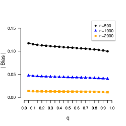
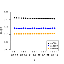
where are iid standard normal variables, is the th quantile of a , and by the Central Limit Theorem. By (38) above, for fixed and and as , meaning that the specific choice of becomes inconsequential when , and thus , is large. Figure 5 shows this empirically — TFB-K’s bias and RMSE in DGP 1 become stable across as increases. However, with smaller , there is a bias-variance trade-off — bias decreases as increases, due to the higher emphasis on reducing imbalance in , but the RMSE is mostly unchanged, implying a higher variance esimator. See Appendices B.5 and B.6, respectively, for similar findings for TFB-K in an extension to DGP 1 that has heteroscedastic error, and DGP 2.
Now consider the setting where is fixed. This will never be the case for TFB-K, but applies to TFB-L in cases where one would not expand were their sample size to grow, and simply would like to take advantage of the LASSO’s variable selection. In this setting, quite generally, so TFB will devalue overall balance in as grows. A near 1 may thus be preferable in this case because it will yield better balance on , which may be valuable if has been misspecified (i.e., is not linear in ). Therefore, because appears to be inconsequential in the case where , and near 1 is advisable when is fixed, seems a reasonable choice.
4.5 Connection to augmented estimation
That TFB allows to inform its weights is key to its merits. However, using estimates of in conjunction with weights, even honest ones, is not novel — it is essential for the augmented (weighted) estimator, the typical form of estimators that do so (e.g., Abadie and Imbens,, 2011; Chernozhukov et al.,, 2018; Athey et al.,, 2018; Hirshberg and Wager,, 2021). This section thus explores the connection between TFB and the augmented estimator.
Recall from Section 3.1 that the expectation of the EWC Bias is exactly the bias of . Consider then bias-correcting by estimating the EWC Bias with a , and subtracting the resulting estimate from :
| (39) |
is the augmented estimator, and the common form of doubly-robust estimators (Robins et al.,, 1994; Robins and Rotnitzky,, 1995; van der Laan and Rubin,, 2006; Chernozhukov et al.,, 2018), which employ propensity score weights, and are consistent when or has been correctly specified.131313Tan, (2010) provides an illuminating review of doubly robust estimators that can be expressed as . Augmented estimators have also been applied with approximate balancing weights (e.g. Athey et al.,, 2018, Hirshberg and Wager,, 2021), and synthetic control (Ben-Michael et al., 2021b, ).
Noting that in TFB reveals its connection to augmented estimators, as the estimated EWC Bias subtracted from to form is
| (40) |
the magnitude of which TFB penalizes. Therefore, often, in TFB, implying . Figure 6 confirms this suspicion in DGPs 1 and 2 — TFB’s augmented and weighted difference in means estimators are numerically identical.
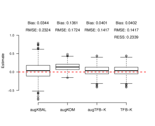
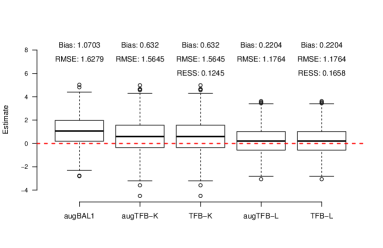
Figure 6 also shows that TFB still achieves lower RMSE than do augmented forms of the estimators examined in Figure 2(a) and 3(a), among them special cases of the estimators studied by Athey et al., (2018) and Hirshberg and Wager, (2021), though the gap in performance has shrunk.141414The residualBalance.ate function in R (from the balanceHD package) is used to implement augBAL1.
That TFB is often approximately equal to an augmented estimator in practice reveals an important connection to the “augmented minimax linear estimator” explored by Hirshberg and Wager, (2021). This class of estimator can be expressed as with BAL2 weights with and a general .151515Hirshberg and Wager, (2021) describe as a function space that contains the difference between a and (i.e., ), rather than itself. However, because is left general, this is ultimately only a difference in framing. Recall that TFB chooses BAL2 weights as well with and . Thus, it seems plausible that TFB is asymptotically equivalent to an augmented minimax linear estimator with the same and .
4.6 Variance estimation and confidence intervals
Given that TFB’s weights are continuous, a bootstrap may be valid for variance estimation and confidence intervals. However, because high-dimensional regression estimators are recommended for TFB, the computation time required for a bootstrap may be impractical. This section thus proposes a closed-form estimated variance, and resulting confidence interval, for TFB. Asymptotic validity is not formally proven, but it is shown to perform well in DGPs 1 and 2 above.
Conditions for the asymptotic normality of a general and a consistent variance estimator
First, consider sufficient conditions for the asymptotic normality of for general weights estimated from the data:
Theorem 1 (Conditions for asymptotic normality of a general )
Given Assumption 1, further assume the following conditions: (i) for a function ;
(ii) ;
(iii) such that ;
(iv) ; (v) such that
and (vi) . Then, where
Proof is given in Appendix C.1. Condition (i) requires that not depend on the given and . Conditions (ii) and (v) then restrict how extreme the can be in asymptopia. Conditions (iii) and (v) restrict the moments of , and condition (iv) restricts the variance of the individual-specific treatment effects (i.e. ). Finally, condition (vi) is key to the -consistency of a , requiring that the bias of converges in probability to 0 at a fast enough rate.
Note again that Theorem 1 does not specify the conditions under which TFB is asymptotically normal, but rather when a with general weights is asymptotically normal. Nevertheless, it is worthwhile discussing conditions (i) and (vi) in the context of TFB. First, note that condition (i) would be satisfied with honest weights, but is violated by TFB as defined. However, sample splitting, as in Chernozhukov et al., (2018), allows condition (i) to hold individually within each of two splits of the sample. The proposed variance estimator leverages this fact, as will be detailed later. Next, it should be emphasized that condition (vi) is far from trivial — for example, Abadie and Imbens, (2006) show it does not hold generally for the matching estimators they examine if . However, there is precedent for balancing weights estimators, and particularly augmented estimators, satisfying this condition under additional assumptions (e.g., Athey et al.,, 2018; Hirshberg and Wager,, 2021). In particular, the close connection between TFB and augmented minimax estimation may imply asymptotic normality under assumptions similar to those proven in Hirshberg and Wager, (2021), among them that has several consistency properties for . Hirshberg and Wager, (2021) also make assumptions on the function space for the BAL2 weights they examine. Thus, because (along with ) determines the analogous for TFB, the properties of likely also play a role here. Further, although it does not appear that complete overlap in the conditional distributions of (as in (18)) is essential (see Appendix B.4), assurance that there exist weights that satisfy EWC in asymptopia would likely be required. Proving the exact assumptions needed for TFB to satisfy condition (vi), along with conditions (ii) and (v), is left to future work. Nevertheless, Theorem 1, and Theorem 2 below, still suggest a closed-form variance estimator.
Turning back to general weights that are estimated from the data, assuming that is a consistent estimator of suggests the plug-in estimator for ,
| (41) |
where . Theorem 2 describes conditions under which .
Theorem 2 (Consistency of )
See Appendix C.2 for proof. Conditions (vii) and (ix) quantify how accurate an estimator of that must be in terms of unweighted and -weighted mean squared error, respectively. Additionally, conditions (viii) and (ix) allow to be robust to heteroscedastic .
Sample splitting, and proposed variance estimator and confidence interval
Theorems 1 and 2 suggest as a variance estimator for TFB. However, TFB violates condition (i) from Theorem 1 as defined. I propose sample splitting to address this, and thus sample splitting was done in all demonstrations of TFB here.
Sample splitting with TFB requires randomly splitting the full sample into two non-overlapping (sub-)samples: Samples 1 and 2. Let the superscripts and denote values that come from Samples 1 and 2, respectively (e.g., . First, use Sample 2 to obtain , and apply them to TFB in Sample 1 to form and . Next, switch the roles of the two sub-samples to obtain from Sample 1, and and from Sample 2. The final estimate is then the average of the estimates from each sub-sample:
| (42) |
With sample splitting, condition (i) from Theorem 1 holds for the estimator from each sub-sample, with respective variances and . Then, following Theorem 2, let and be the variance estimators from the two sub-samples. This leads to the proposed variance estimator:
| (43) |
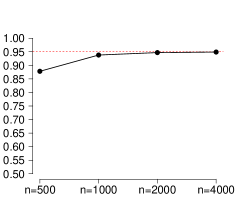
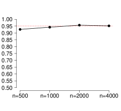
confidence intervals can then be obtained using the normal approximation: . Figure 7 shows that 95% confidence intervals with the proposed variance estimator achieve essentially 95% coverage as increases. The undercoverage for TFB-K when in DGP 1 is likely because TFB-K still shows bias at that sample size (see Figure 5). Note that in extensions to DGPs 1 and 2 in Appendices B.1 and B.2 that vary aspects of the DGPs (e.g., , overlap, and sample size), the proposed confidence intervals reach, or fall just below, the target coverage rate of 95% when TFB’s bias is low.
Note that the asymptotic validity of in (43) (given the other conditions from Theorems 1 and 2) requires that the estimates from each sub-sample are asymptotically uncorrelated. Proving this is left to future work, but Table 2 demonstrates that it is plausible, despite the estimates’ being correlated in finite samples (the in Sample 1 contribute to from Sample 2, and vice versa). The correlation between the estimates appears to disappear as increases in DGPs 1 and 2.
| DGP 1 (TFB-K) | 0.103* | 0.076* | 0.037 | 0.011 |
|---|---|---|---|---|
| DGP 2 (TFB-L) | 0.104* | 0.07* | -0.008 | 0.005 |
Finally, when sample-splitting in real-data applications, it is prudent to examine estimates from many random splits of the sample. However, if a single estimate is required for reporting, Chernozhukov et al., (2018) suggest the median. Let be the TFB estimate from the th split of the sample and let consistently estimate its variance. Then, let be the median of the . Results from Chernozhukov et al., (2018) imply the variance estimator
| (44) |
% confidence intervals can be obtained through the normal approximation: .
5 Application
This section assesses TFB’s performance on the National Supported Work (NSW) Demonstration data, accessible from Dehejia, (2023). NSW was a labor training program in the mid-1970s that randomly selected its participants from a group of candidates. In addition to experimental treated and control groups drawn from the program candidates, data on comparison groups of non-candidates are available. LaLonde, (1986) and Dehejia and Wahba, (1999) use these data to compare non-experimental estimates of NSW’s impact on 1978 earnings (the outcome here) to the unbiased experimental estimate. Defining the treated (185 units), experimental control (260), and non-candidate comparison (2,490) groups as in Dehejia and Wahba, (1999) yields an experimental estimate of $1,794 and a naive observational estimate (i.e., the unweighted difference in means between the experimental treated and non-candidate comparison groups) of -$15,205.
The available covariates are age, years of education, an indicator of having a high school degree, 1974 and 1975 earnings, indicators of unemployment in 1974 and 1975, marital status, and several indicators of race/ethnicity. Figure 8 compares TFB-L, where is estimated by LASSO regression, and TFB-K, where is estimated by kernel regularized least squares, to seven other estimators.
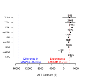
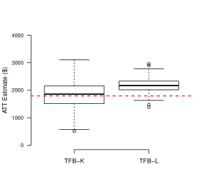
The first of these estimators is Entropy Balancing (EBAL; Hainmueller,, 2012), which is an exact balancing method (see Section 3.2). The next three estimators are the same approximate balancing methods that were used in the demonstrations from Section 4.3: BAL1 where all the are equal (see Section 3.2), Kernel Balancing (KBAL; Hazlett,, 2020), and Kernel Optimal Matching (KOM; Kallus,, 2020). The final three estimators are augmented forms (see Section 4.5) of the three approximate balancing methods.161616The ebalance function in R (from the ebal package) was used to implement EBAL. Each other method’s specifics are consistent with Sections 4.3 and 4.5. The kernel-based approximate balancing methods (i.e., TFB-K, KBAL, and KOM) use the Gaussian kernel with bandwidth , and their corresponding augmented forms use from kernel regularized least squares. augABAL uses from LASSO regression. TFB-K uses from (29) and TFB-L finds by residual bootstrapping. Both TFB-K and TFB-L set , per Section 4.4. TFB-K, EBAL, (aug)KBAL, and (aug)KOM are limited to the 10 untransformed covariates, while (aug)BAL1 and TFB-L additionally use the covariates’ squared terms and pairwise interactions, a total of 52 covariates.171717Following Hainmueller, (2012), I exclude various squares and interactions. These are the interaction between the indicator for high school degree and years of education, the interactions of the race/ethnicity indicators, and the squares and interactions of real earnings in 1974 and 1975. TFB-L and TFB-K both employ sample splitting here (see Section 4.6), so estimates across 100 random splits of the sample are provided in Figure 8(b), and Figure 8(a) reports the median estimate.
As are the other estimators, TFB-K and TFB-L are large improvements over the naive estimate of -$15,205, and are the first and fifth closest (of nine), respectively, to the experimental benchmark. However, as this is just one realization of the data, drawing conclusions from these minute differences is challenging. It is more affirming that TFB performs comparably to other well-known estimators and that the experimental estimate falls within TFB-K’s and TFB-L’s 95% confidence intervals (as do the other estimators excluding augBAL1).
Finally, Table 3(a) reports the standardized imbalance in the covariates for each weighting method.
| Partial Corr. | Initial Imbal. | TFB-K | TFB-L | EBAL | BAL1 | KBAL | KOM | |
| Age | -0.08 | -0.86 | -0.13 | -0.33 | 0 | -0.03 | -0.1 | -0.11 |
| Years of Education | 0.11 | -0.58 | -0.05 | 0.04 | 0 | -0.05 | 0 | -0.03 |
| Ethnicity (Black) | -0.02 | 1.3 | 0.08 | 0.17 | 0 | 0.05 | 0.03 | 0.05 |
| Ethnicity (Hispanic) | 0.04 | 0.15 | 0.04 | 0.06 | 0 | 0.05 | -0.06 | 0.02 |
| Married | 0.04 | -1.76 | -0.08 | -0.23 | 0 | -0.06 | -0.04 | -0.06 |
| No HS Degree | 0.02 | 0.85 | 0.06 | 0.05 | 0 | 0.06 | 0.06 | 0.05 |
| Earnings (1974) | 0.18 | -1.26 | -0.01 | 0.01 | 0 | -0.02 | 0 | -0.05 |
| Earnings (1975) | 0.32 | -1.26 | -0.03 | -0.01 | 0 | -0.06 | 0.01 | -0.07 |
| Unemployed (1974) | 0.02 | 1.85 | 0.02 | 0.06 | 0 | 0.06 | 0 | 0.08 |
| Unemployed (1975) | -0.03 | 1.46 | -0.02 | -0.06 | 0 | 0.06 | -0.01 | 0.02 |
TFB shows similar tendencies here as in previous demonstrations. TFB obtains very good balance on 1974 and 1975 earnings, which have the highest partial correlations with the outcome. Furthermore, because TFB-K does not estimate with sparsity, TFB-K obtains good balance in all of the covariates, even those with low partial correlation with the outcome. Meanwhile, TFB-L leaves imbalance in age, the indicator of being Black, and the indicator of being married, the latter two of which show low partial correlation with the outcome.
6 Conclusion
This paper has introduced TFB, an approximate balancing framework that first regresses the outcome on the observed covariates, and then uses the resulting regression function and its estimated variance to determine how to balance the covariates. As a result, TFB seeks balance in the predicted values of the regression function and in the covariates, allowing the regression function’s variance to determine how much of the latter is necessary. In simulated examples, TFB showed promising results when compared to applications of existing approximate balancing methods that disregarded the outcome (i.e., are “honest”) and any potential background knowledge (e.g., which covariates are most influential on the outcome) when balancing the covariates. In real-data scenarios, investigators could apply background knowledge to tune these methods, potentially closing any performance gap that might exist between these methods and TFB. Nevertheless, TFB’s advantage is that the choice of regression estimator and an estimator for its variance entirely determines how it balances the covariates. This turns the problem of how best to balance the covariates into how best to model the outcome. TFB does, however, require different weights for different outcomes. This is a practical disadvantage in that it complicates analyses, and can be time-consuming. But it is also a potential advantage, particularly in settings with minimal overlap in the covariates — while it may be impossible to find a single set of weights that is appropriate for all outcomes, TFB may be able to find a different sets of weights that are individually appropriate for some (or all) of the outcomes.
One consequence of TFB is that it may intentionally leave imbalance in the covariates even when exact balance is feasible, either because certain dimensions appear conditionally unrelated to the outcome, or even to use imbalances in some dimensions to offset imbalances in others. Intentional imbalance is not a novel idea — several existing methods also leave imbalance in the name of variance reduction (e.g., Zubizarreta,, 2015) or to prioritize balance in more predictive dimensions (e.g., Ning et al.,, 2020). However, the motivation behind this characteristic of TFB does challenge traditional advice (e.g., Stuart,, 2010) that the ultimate goal of weighting is to equate the distributions of the covariates in the treated and control groups, with a particular focus on mean balance in the covariates as a benchmark for success. TFB instead argues that any balance in the covariates should only be a byproduct of balance in , which is all that is required for unbiased estimation. It is understandable to be suspicious of this perspective in practice, given TFB’s reliance on a , not . However, note that it is theoretically sound, and is shown here to potentially yield efficiency gains. Further, recall that TFB still does value overall balance in the covariates, using it to safeguard against an over-reliance on .
As for implementation, TFB is recommended in high-dimensional settings, particularly the forms that use kernel regularized least squares to regress the outcome, or an estimator that induces sparsity, such as the LASSO. However, I do not recommend a form of TFB that regresses the outcome with OLS in a low-dimensional setting. Furthermore, when applying TFB, a probability threshold () close to 1 is recommended (e.g., ). I also suggest performing sample splitting, calculating estimates across multiple random splits of the sample, and ultimately reporting the median. As for diagnostics, I suggest confirming that TFB obtains good balance on variables one would expect are the most influential on the outcome (determined by content knowledge or partial correlation), and that the variables with more imbalance are those that are expected to be less influential on the outcome. Note also that while this paper has framed TFB as an estimator for the average treatment effect on the treated (ATT), Appendix A adapts it to estimate the average treatment effect (ATE) and the average treatment effect on the controls (ATC).
There are several avenues for future work. First, although this paper has demonstrated TFB’s merits in finite samples, proving its asymptotic properties would be a major contribution. The connection between TFB and augmented minimax linear estimation studied by Hirshberg and Wager, (2021) may be key here. Ben-Michael et al., 2021a , which studies the asymptotic properties of estimators that use balancing weights, may also be helpful. Second, this paper has focused on forms of TFB that use a regression estimator with a linear representation (i.e., ). Extending TFB so it may use regression estimators that do not have a linear representation (e.g., generalized linear models or tree-based methods) would be worthwhile, given the popularity of such models. Third, TFB was compared to honest weighting procedures in all demonstrations here. Comparing TFB to other procedures that allow the outcome to inform the weights (e.g., Tan,, 2010; Rotnitzky et al.,, 2012; Shortreed and Ertefaie,, 2017; Ning et al.,, 2020; Kuang et al.,, 2017) would be extremely interesting. Finally, this paper has also introduced TFI, a balance diagnostic that TFB minimizes over weights, subject to constraints on their variance. However, this is not TFI’s only possible application. It could incorporated into best subset matching (e.g., Nikolaev et al.,, 2013), where TFI (and other components) would be minimized over for some whole number . TFI could also be integrated into a loss function used to estimate the parameters for a propensity score (e.g., Zhao,, 2019; Pirracchio and Carone,, 2018). The resulting propensity score weighted estimator might then be doubly robust. TFI might also have uses in other methods, such as a diagnostic for choosing the dimension of the approximation of the gram matrix in Kernel Balancing (Hazlett,, 2020). Note, however, that because TFI is a function of the outcomes, incorporating it would make an otherwise honest weighting procedure non-honest. As seen in Section 4.6, this could have implications for asymptotic behavior, which should be studied before committing to integrating TFI.
References
- Abadie and Imbens, (2006) Abadie, A. and Imbens, G. W. (2006). Large sample properties of matching estimators for average treatment effects. Econometrica, 74(1):235–267.
- Abadie and Imbens, (2011) Abadie, A. and Imbens, G. W. (2011). Bias-corrected matching estimators for average treatment effects. Journal of Business & Economic Statistics, 29(1):1–11.
- Antonelli et al., (2018) Antonelli, J., Cefalu, M., Palmer, N., and Agniel, D. (2018). Doubly robust matching estimators for high dimensional confounding adjustment. Biometrics, 74(4):1171–1179.
- Athey et al., (2018) Athey, S., Imbens, G. W., and Wager, S. (2018). Approximate residual balancing: Debiased inference of average treatment effects in high dimensions. Journal of the Royal Statistical Society: Series B (Statistical Methodology), 80(4):597–623.
- (5) Ben-Michael, E., Feller, A., Hirshberg, D. A., and Zubizarreta, J. R. (2021a). The balancing act in causal inference. arXiv preprint arXiv:2110.14831.
- (6) Ben-Michael, E., Feller, A., and Rothstein, J. (2021b). The augmented synthetic control method. Journal of the American Statistical Association, 0(0):1–15.
- Chan et al., (2016) Chan, K. C. G., Yam, S. C. P., and Zhang, Z. (2016). Globally efficient non-parametric inference of average treatment effects by empirical balancing calibration weighting. Journal of the Royal Statistical Society: Series B (Statistical Methodology), 78(3):673–700.
- Chatterjee and Lahiri, (2010) Chatterjee, A. and Lahiri, S. N. (2010). Asymptotic properties of the residual bootstrap for lasso estimators. Proceedings of the American Mathematical Society, 138(12):4497–4509.
- Chatterjee and Lahiri, (2011) Chatterjee, A. and Lahiri, S. N. (2011). Bootstrapping lasso estimators. Journal of the American Statistical Association, 106(494):608–625.
- Chattopadhyay et al., (2020) Chattopadhyay, A., Hase, C. H., and Zubizarreta, J. R. (2020). Balancing versus modeling approaches to weighting in practice. Statistics in Medicine, 39(24):3227–3254.
- Chernozhukov et al., (2018) Chernozhukov, V., Chetverikov, D., Demirer, M., Duflo, E., Hansen, C., Newey, W., and Robins, J. (2018). Double/debiased machine learning for treatment and structural parameters. Econometrics Journal, 21(1):C1–C68.
- Dehejia, (2023) Dehejia, R. (2023). data download. https://users.nber.org/~rdehejia/data/.nswdata2.html. Accessed: 2023-06-26.
- Dehejia and Wahba, (1999) Dehejia, R. H. and Wahba, S. (1999). Causal effects in nonexperimental studies: Reevaluating the evaluation of training programs. Journal of the American Statistical Association, 94(448):1053–1062.
- Deming and Stephan, (1940) Deming, W. E. and Stephan, F. F. (1940). On a least squares adjustment of a sampled frequency table when the expected marginal totals are known. The Annals of Mathematical Statistics, 11(4):427–444.
- Deville and Särndal, (1992) Deville, J.-C. and Särndal, C.-E. (1992). Calibration estimators in survey sampling. Journal of the American Statistical Association, 87(418):376–382.
- Hainmueller, (2012) Hainmueller, J. (2012). Entropy balancing for causal effects: A multivariate reweighting method to produce balanced samples in observational studies. Political Analysis, 20(1):25–46.
- Hainmueller and Hazlett, (2014) Hainmueller, J. and Hazlett, C. (2014). Kernel regularized least squares: Reducing misspecification bias with a flexible and interpretable machine learning approach. Political Analysis, 22(2):143–168.
- Hansen, (2008) Hansen, B. B. (2008). The prognostic analogue of the propensity score. Biometrika, 95(2):481–488.
- Hazlett, (2020) Hazlett, C. (2020). Kernel balancing: A flexible non-parametric weighting procedure for estimating causal effects. Statistica Sinica, 30(1):1155–1189.
- Hirshberg et al., (2021) Hirshberg, D. A., Maleki, A., and Zubizarreta, J. R. (2021). Minimax linear estimation of the retargeted mean. arXiv preprint arXiv:1901.10296v2.
- Hirshberg and Wager, (2021) Hirshberg, D. A. and Wager, S. (2021). Augmented minimax linear estimation. The Annals of Statistics, 49(6):3206–3227.
- Hong et al., (2021) Hong, G., Yang, F., and Qin, X. (2021). Did you conduct a sensitivity analysis? a new weighting-based approach for evaluations of the average treatment effect for the treated. Journal of the Royal Statistical Society Series A: Statistics in Society, 184(1):227–254.
- Huang et al., (2006) Huang, J., Smola, A. J., Gretton, A., Borgwardt, K. M., and Schölkopf, B. (2006). Correcting sample selection bias by unlabeled data. Advances in Neural Information Processing Systems, 19:601–608.
- Imai and Ratkovic, (2014) Imai, K. and Ratkovic, M. (2014). Covariate balancing propensity score. Journal of the Royal Statistical Society: Series B (Statistical Methodology), 76(1):243–263.
- Kallus, (2020) Kallus, N. (2020). Generalized optimal matching methods for causal inference. Journal of Machine Learning Research, 21:1–54.
- Kang and Schafer, (2007) Kang, J. D. Y. and Schafer, J. L. (2007). Demystifying double robustness: A comparison of alternative strategies for estimating a population mean from incomplete data. Statistical Science, 22(4):523–539.
- Knight and Fu, (2000) Knight, K. and Fu, W. (2000). Asymptotics for lasso-type estimators. The Annals of Statistics, 28(5):1356–1378.
- Kuang et al., (2017) Kuang, K., Cui, P., Li, B., Jiang, M., and Yang, S. (2017). Estimating treatment effect in the wild via differentiated confounder balancing. In Proceedings of the 23rd ACM SIGKDD International Conference on Knowledge Discovery and Data Mining, pages 265–274.
- LaLonde, (1986) LaLonde, R. J. (1986). Evaluating the econometric evaluations of training programs with experimental data. The American Economic Review, 76(4):604–620.
- Leacy and Stuart, (2014) Leacy, F. P. and Stuart, E. A. (2014). On the joint use of propensity and prognostic scores in estimation of the average treatment effect on the treated: A simulation study. Statistics in Medicine, 33(20):3488–3508.
- Nikolaev et al., (2013) Nikolaev, A. G., Jacobson, S. H., Cho, W. K. T., Sauppe, J. J., and Sewell, E. C. (2013). Balance optimization subset selection (BOSS): An alternative approach for causal inference with observational data. Operations Research, 61(2):398–412.
- Ning et al., (2020) Ning, Y., Peng, S., and Imai, K. (2020). Robust estimation of causal effects via a high-dimensional covariate balancing propensity score. Biometrika, 107(3):533–554.
- Pirracchio and Carone, (2018) Pirracchio, R. and Carone, M. (2018). The balance super learner: A robust adaptation of the super learner to improve estimation of the average treatment effect in the treated based on propensity score matching. Statistical Methods in Medical Research, 27(8):2504–2518.
- Robins and Rotnitzky, (1995) Robins, J. M. and Rotnitzky, A. (1995). Semiparametric efficiency in multivariate regression models with missing data. Journal of the American Statistical Association, 90(429):122–129.
- Robins et al., (1994) Robins, J. M., Rotnitzky, A., and Zhao, L. P. (1994). Estimation of regression coefficients when some regressors are not always observed. Journal of the American Statistical Association, 89(427):846–866.
- Rosenbaum and Rubin, (1983) Rosenbaum, P. R. and Rubin, D. B. (1983). The central role of the propensity score in observational studies for causal effects. Biometrika, 70(1):41–55.
- Rotnitzky et al., (2012) Rotnitzky, A., Lei, Q., Sued, M., and Robins, J. M. (2012). Improved double-robust estimation in missing data and causal inference models. Biometrika, 99(2):439–456.
- Rubin, (1974) Rubin, D. B. (1974). Estimating causal effects of treatments in randomized and nonrandomized studies. Journal of Educational Psychology, 66(5):688–701.
- Schölkopf and Smola, (2002) Schölkopf, B. and Smola, A. J. (2002). Learning with kernels: Support vector machines, regularization, optimization, and beyond. MIT Press.
- Shortreed and Ertefaie, (2017) Shortreed, S. M. and Ertefaie, A. (2017). Outcome-adaptive lasso: Variable selection for causal inference. Biometrics, 73(4):1111–1122.
- Soriano et al., (2021) Soriano, D., Ben-Michael, E., Bickel, P. J., Feller, A., and Pimentel, S. D. (2021). Interpretable sensitivity analysis for balancing weights. arXiv preprint arXiv:2102.13218.
- Splawa-Neyman et al., (1990) Splawa-Neyman, J., Dabrowska, D. M., and Speed, T. (1990). On the application of probability theory to agricultural experiments. Essay on principles. Section 9. Statistical Science, 5(4):465–472.
- Stuart, (2010) Stuart, E. A. (2010). Matching methods for causal inference: A review and a look forward. Statistical Science, 25(1):1–21.
- Tan, (2010) Tan, Z. (2010). Bounded, efficient and doubly robust estimation with inverse weighting. Biometrika, 97(3):661–682.
- Tarr and Imai, (2021) Tarr, A. and Imai, K. (2021). Estimating average treatment effects with support vector machines. arXiv preprint arXiv:2102.11926v2.
- van der Laan and Rubin, (2006) van der Laan, M. J. and Rubin, D. (2006). Targeted maximum likelihood learning. The International Journal of Biostatistics, 2(1):1–38.
- Wainwright, (2019) Wainwright, M. J. (2019). High-dimensional statistics: A non-asymptotic viewpoint. Cambridge University Press, first edition.
- Wang and Zubizarreta, (2020) Wang, Y. and Zubizarreta, J. R. (2020). Minimal dispersion approximately balancing weights: Asymptotic properties and practical considerations. Biometrika, 107(1):93–105.
- White, (1980) White, H. (1980). A heteroskedasticity-consistent covariance matrix estimator and a direct test for heteroskedasticity. Econometrica, 48(4):817–838.
- Wong and Chan, (2018) Wong, R. K. W. and Chan, K. C. G. (2018). Kernel-based covariate functional balancing for observational studies. Biometrika, 105(1):199–213.
- Zhao, (2019) Zhao, Q. (2019). Covariate balancing propensity score by tailored loss functions. The Annals of Statistics, 47(2):965–993.
- Zubizarreta, (2015) Zubizarreta, J. R. (2015). Stable weights that balance covariates for estimation with incomplete outcome data. Journal of the American Statistical Association, 110(511):910–922.
Appendix A Extensions to the ATC and the ATE
Although this paper describes TFI and TFB in the context of estimating the ATT, they are both easily extended to estimate the ATC and the ATE. This appendix details how to do so. Although it is a slight abuse of notation, let be a general vector of positive weights. When in the context of the ATC, these weights will only be defined for treated units. When in the context of the ATE, these weights will be defined for the full sample.
A.1 Weighted difference in mean estimators for the ATC and the ATE
I first define the weighted difference in means estimators that will be used to estimate the ATC and the ATE.
ATC
A weighted difference in means estimator for the ATC takes the form
| (45) |
where all and, often, .
ATE
A weighted difference in means estimator for the ATE takes the form
| (46) |
where all and, often, and .
A.2 TFI for the ATC and the ATE
This section extends TFI to weighted difference in means estimators of the ATC and the ATE. Like when estimating the ATT, these extensions of TFI are approximations of the bias of and in estimating the ATC and ATE, respectively.
First, however, we require extra notation. Define
| (47) |
where is an arbitrary vector-valued function. In words, is the imbalance in between the unweighted control group and the weighted treated group. Then, define
| and | (48) |
In words, is the imbalance in between the full sample and the weighted group with treatment status . Finally, let for be the coefficients from regression estimators , and let be estimates of their variances.
ATC
TFI for a is defined as
| (49) |
As before, is a probability threshold chosen by the researcher.
ATE
Define TFI for a as
| (50) |
Again, is a probability threshold chosen by the user.
A.3 TFB for the ATC and the ATE
This section details how TFB finds weights to estimate the ATC and the ATE.
ATC
Similar to when estimating the ATT, TFB chooses weights to estimate the ATC that minimize the corresponding TFI subject to constraints on the weights’ variance. In other words,
| where | (51) |
where .
ATE
To estimate the ATE, TFB chooses
| where | (52) |
where and .
A.4 Variance estimation for the ATC and the ATE
Finally, this section proposes variance estimators for TFB estimators of the ATC and ATT.
ATC
Theorem 3 describes sufficient conditions to determine the asymptotic normality of a with general weights estimated from the data. Then, Theorem 4 introduces an estimator of the asymptotic variance of and describes sufficient conditions for the estimator’s consistency.
Theorem 3 (Conditions for asymptotic normality of a general )
Given Assumption 1, further assume the following conditions: (i) for a function ; (ii) ; (iii) such that ; (iv) ; (v) such that
and (vi) . Then, where
Theorem 4 (Estimating )
The proofs for Theorems 3 and 4 are omitted here because the ATC is simply the negative of the ATT for the reversed treatment, , and potential outcomes, (i.e., . Therefore, the proofs for Theorems 3 and 4 follow nearly identical steps to those for Theorems 1 and 2 (in Appendices C.1 and C.2), respectively.
I emphasize that Theorems 3 and 4 are for an estimator with general weights, not TFB specifically. However, as with the ATT, these theorems provide motivation for a closed-form variance estimator for TFB. I again propose sample splitting. First, randomly split the full sample into two non-overlapping (sub-)samples: Samples 1 and 2. Use Sample 2 to obtain , and apply them to TFB in Sample 1 to form and . Next, switch the roles of the two sub-samples to obtain from Sample 1, and from Sample 2. The final estimate is then average of the estimates from each sub-sample:
| (53) |
The proposed variance estimator is then:
| (54) |
confidence intervals can then be obtained using the normal approximation: .
ATE
Theorem 5 describes sufficient conditions to determine the asymptotic normality of a with general weights estimated from the data. Then, Theorem 6 introduces an estimator of the asymptotic variance of and describes sufficient conditions for the estimator’s consistency.
Theorem 5 (Conditions for asymptotic normality of a general )
Given Assumption 1, further assume the following conditions: (i) for a function ; (ii) and ; (iii) such that and ; (iv) ; (v) such that
and (vi) and . Then, where
Theorem 6 (Estimating )
I emphasize that Theorems 5 and 6 are for an estimator with general weights, not TFB specifically. However, as with the ATT, these theorems provide motivation for a closed-form variance estimator for TFB. I again propose sample splitting. First, randomly split the full sample into two non-overlapping (sub-)samples: Samples 1 and 2. Use Sample 2 to obtain , and apply them to TFB in Sample 1 to form and . Next, switch the roles of the two sub-samples to obtain from Sample 1, and from Sample 2. The final estimate is then average of the estimates from each sub-sample:
| (55) |
The proposed variance estimator is then:
| (56) |
confidence intervals can then be obtained using the normal approximation: .
Appendix B Simulations
B.1 Extension to DGP 1
This section investigates how TFB-K performs after varying important aspects of DGP 1 from Section 4.3. As in DGP 1, is drawn from a bivariate normal distribution around , one of four equally likely (cluster) centers that are unknown to the researcher,
| (57) |
Though and again depend on for ,
| (58) |
which are unknown to the researcher.
Several aspects of the probability of treatment and model for the outcome are varied. The probability of treatment is:
| (59) |
where , the coefficient on , takes values . controls the extent of overlap in the distributions of between the treated and control groups — grants the most overlap, grants the least overlap, and grants medium overlap. The level of overlap for , , and is not varied here because the goal is to see if TFB still leaves imbalance in to overcome low overlap in the other for different levels of overlap in .
The model for the outcome is:
| (60) |
where , the variance of the error term , is varied so that the model takes values in (60) The is varied to see how the maximum predictive power of a influences TFB-K’s performance. Finally, two sample sizes are tried: To summarize, the following aspects are varied:
-
•
in (59)
-
•
-
•
Note that , and essentially recreates DGP 1 in Section 4.3.
As in Section 4.3, TFB-K is compared to to Kernel Balancing (KBAL; Hazlett,, 2020) and Kernel Optimal Matching (KOM; Kallus,, 2020). All methods are implemented in the same way as in Section 4.3. Also included in the comparison are the augmented forms of KBAL (augKBAL) and KOM (augKOM), both using kernel regularized least squares as their regression function, as in Section 4.5. Figure 9(g) reports the RMSE of each estimator, Figure 10(g) reports the bias, Figure 11(g) reports the median imbalance in , and Figure 12(g) reports the coverage rate of 95% confidence intervals found through the proposal in Section 4.6 across the 200 iterations from each setting.
Starting with RMSE in Figure 9(g), as expected, the RMSE for each method tends to increase as overlap in decreases (i.e., increases), and RMSE tends to decrease as and increase. The exceptions are KBAL and augKBAL, whose RMSEs are fairly consistent as and overlap change. In the vast majority of settings, TFB-K has the lowest RMSE. augKOM has the second lowest RMSE in the large majority of settings.
Figure 10(g) shows that TFB-K does not always have the least bias in every setting — KBAL tends to have the least bias, except when with or 0.90 and high or medium overlap. Note also that the settings in which TFB-K shows little to no bias — when there is high or medium overlap combined with and , or — are all settings in which TFB-K’s median imbalance for is negative (see Figure 11(g)), i.e. the opposite sign of the original imbalance. Recall that in the original DGP 1 this allowed TFB-K to be nearly unbiased. That this occurs when the is high and there is high or medium overlap makes sense. When the is high, is more predictive of the outcome and thus has lower variance, meaning TFB-K can more confidently leave imbalance in . Further, when there is high or medium overlap, leaving negative imbalance in does not require outlandishly high variance weights. Finally, Figure 12(g) shows that the proposed confidence intervals for TFB-K from Section 4.6 reach, or fall just below, the target coverage rate of 0.95 in the same settings in which TFB-K shows little bias (i.e., when when there is high or medium overlap combined with and , or ).
In summary, TFB-K performs well even after varying important aspects of DGP 1 — it consistently has the lowest RMSE among the comparison methods tried. It also shows little bias when the model is higher, and there is acceptable overlap in key confounders. When the model and the overlap are lower, TFB-K appears to prioritize lower variance weights, leaving imbalance in confounders that induces bias. However, even in these settings, TFB-K often still has the lowest RMSE. Finally, the proposed confidence intervals from Section 4.6 perform well when TFB-K shows little bias.
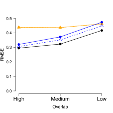
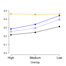
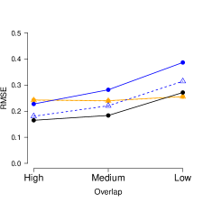
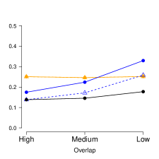
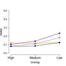
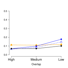
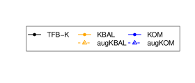
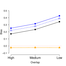
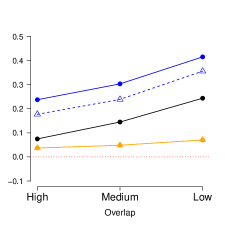
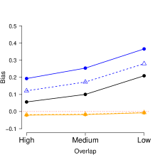
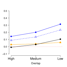
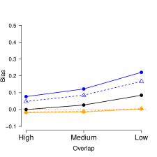
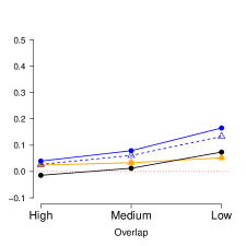

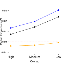
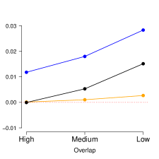
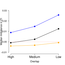
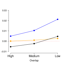
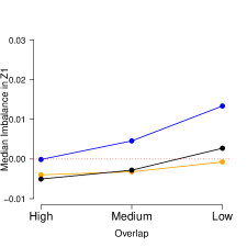
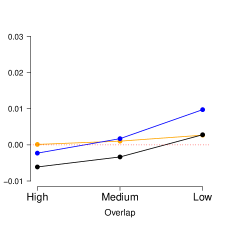


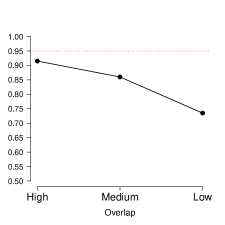
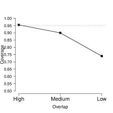
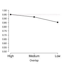
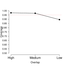

B.2 Extension to DGP 2
This section investigates how TFB performs after varying important aspects of DGP 2 from Section 4.3. As in DGP 2, contains three types of variables: (i) “confounders”, , that are related to both and ; (ii) “distractors”, , that are related to , and are difficult to balance, but are unrelated to ; and (iii) “extraneous” variables, , that are independent of both and . The are again generated as
| (61) |
and the log odds of treatment is again linear in ,
| (62) |
Here, the of the model for the outcome, and the dimensions of the distractor and extraneous variables are varied. First, the outcome is linear in ,
| (63) |
where , the variance of the error term , is varied so that the takes values . The is varied to examine how the maximum predictive power of a influences TFB’s performance.
Then, the distractors () and the extraneous variables () are generated as
| (64) |
where . In other words, I consider settings with distractors and extraneous variables (), distractors and extraneous variables (), and distractors and extraneous variables (). Finally, two samples sizes are tried: To summarize, the following aspects are varied:
Note that , and essentially recreates DGP 2 in Section 4.3.
As in Section 4.3, TFB-L and TFB-K are compared to an application of BAL1 that does not prioritize balance in any dimensions of . All methods are implemented in the same way as in Section 4.3. Note that for TFB-L and BAL1, this involves adding to all its squares and pairwise interactions — when (5 distractors and 10 extraneous variables) this totals 209 variables, when (10 distractors and 20 extraneous variables) this totals 629 variables, and when (15 distractors and 30 extraneous variables) this totals 1274 variables. Also included in the comparison is the augmented form of BAL1 (augBAL1), which uses the LASSO for its regression function, as in Section 4.5. Figure 13(g) reports the RMSE of each estimator, Figure 14(g) reports the bias, and Figure 15(g) reports the coverage rate of 95% confidence intervals found through the proposal in Section 4.6 across 200 iterations from each setting.
Starting with RMSE in Figure 13(g), TFB-L has the lowest RMSE in every setting. TFB-K has about the same, or a slightly higher, RMSE as does augBAL1 in most of the settings, except when and . Figure 14(g) shows that TFB-L consistently has the lowest bias of all of the estimators tried here. However, TFB-L does show bias until . Further, TFB-K has the second lowest bias in most settings, though performs about the same as does augBAL1 when . Finally, Figure 15(g) shows that the proposed confidence intervals for TFB-L from Section 4.6 reach, or fall just below, the target coverage rate of 0.95 when TFB-L’s bias is lowest in Figure 14(g) (i.e., when and , or when ).
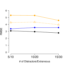
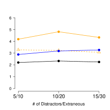
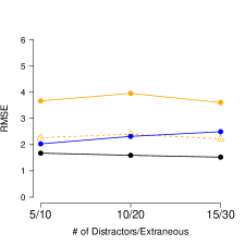
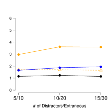
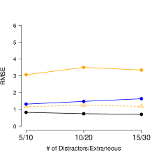
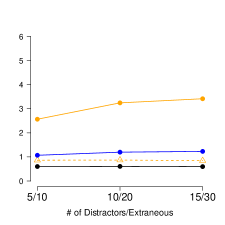

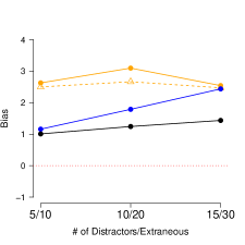
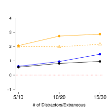
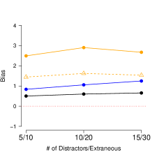
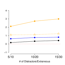
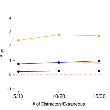
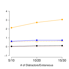
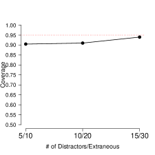
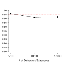

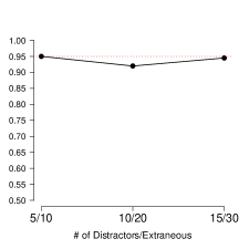
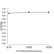
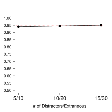
B.3 Danger of misspecifying in TFB
In both DGPs 1 and 2 from Section 4.3, the applications of TFB either correctly specify or (in the case of TFB-K) is well-approximated by a from kernel regularized least squares. This section demonstrates the bias that can occur when TFB-L incorrectly specifies .
An extension to DGP 2 is considered here. As in DGP 2, contains three types of variables: (i) “confounders”, , that are related to both and ; (ii) “distractors”, , that are related to , and are difficult to balance, but are unrelated to ; and (iii) “extraneous” variables, , that are independent of both and . The , , and are again generated as
| (65) |
The difference from DGP 2 comes in the propensity store and model for the outcome. Instead of both the log odds of treatment and being linear in , the key transformation of ,
| (66) |
is very influential in both models:
| (67) | ||||
| (68) |
Centering by 0.66 in the propensity score allows , and choosing allows the model to be approximately 0.50.
As in Section 4.3, TFB-L is compared to an application of BAL1 that does not prioritize balance in any dimensions of . Also included in the comparison is the augmented form of BAL1 (augBAL1), which uses the LASSO for its regression function. All methods are implemented in the same way as in Section 4.3 and 4.5. Note that this involves adding to all its squares and pairwise interactions, which totals 209 variables. However, this does not include , meaning that all methods should expect bias. This bias is confirmed in Figure 16 — all methods, including TFB-L, show noticeable bias at and .
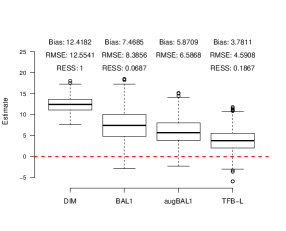
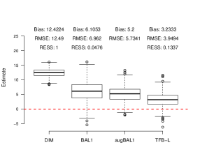
B.4 Obviating complete overlap
Section 3.1 discusses how the traditional assumption of complete overlap in the conditional distributions of , often written as (18), is not required for EWC. In fact all that is needed is for the average in the treated group to be in the range of the in the control group. For example, consider the following DGP:
| where | ||||
| and | (69) |
Here this no overlap in the distribution of — the control group only has values less than 0, and the treated group only has values greater than 0. Thus, both propensity score methods and any balancing method that requires exact balance on would be impossible. However, , and the among the control group have a range of . Thus, EWC is often possible.
Consider now applying TFB to this DGP. Here, for simplicity, TFB will use an OLS that regresses on to estimate , and the sandwich variance estimator ( in (25)). Figure 17 reports TFB’s performance in this DGP, and investigates the leftover imbalance in and after weighting. Despite the lack of overlap in , TFB is effectively unbiased at . Per Figure 17(b), TFB achieves this by inducing imbalance in to offset imbalance in .
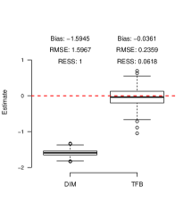
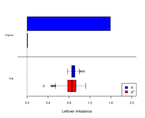
There are a couple things to note. First, note that even though OLS with a small number of regressors was applied here for TFB, I still do not recommend this practice in general. In this example, the OLS perfectly specifies , which is unlikely in practice. However, despite this, it is still an important result that should have implications for the assumptions required for TFB’s asymptotic properties. It is clear that, depending on the consistency of the regression estimator , one may only need a very weak overlap assumption in order for TFB to be asymptotically unbiased.
B.5 Heteroscedastic error in DGP 1
This section considers an extension to DGP 1 from Section 4.3 in which the error in the model for in (33) is heteroscedastic. Here, the , , and are generated exactly as they are in DGP 1. However the model for is now:
| (70) |
where the conditional variance of the is now a function of . Furthermore, dividing by 8 in the variance of results in a true of approximately 0.60, just like in the original DGP 1.
I consider the same estimators in this extension as the demonstrations on DGP 1 in Section 4.3 and 4.5. The goal of this experiment is to see if TFB-K’s performance, which uses in (29) as its variance estimator, is sensitive to heteroscedastic error. As mentioned previously, Hainmueller and Hazlett, (2014) show that is valid only under homoscedastic error.
Figure 18 compares the estimators’ performance in this extension, and investigates the leftover imbalance in the after weighting. As in Section 4.3 and 4.5, TFB-K still has the lowest RMSE and shows little bias. Further, comparing Figure 18(b) to Figure 2(b), we see that TFB-K shows similar tendencies in the original DGP 1 and this extension — it leaves imbalance in of the opposite sign to offset imbalance in the other . Figure 19 then examines the bias and RMSE of TFB-K in this extension for varying . Comparing Figure 19 to Figure 5, we again see very similar trends. With smaller , there a bias-variance trade-off in that the bias decreases as increases, but the RMSE is relatively stable. When , both the bias and RMSE are quite stable across all values of .
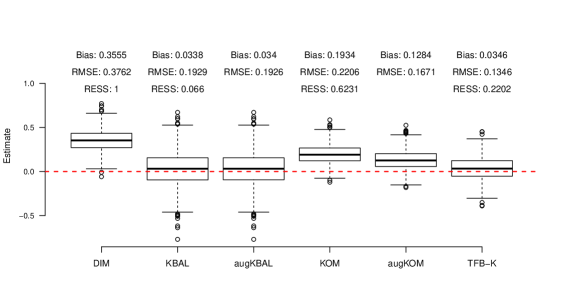
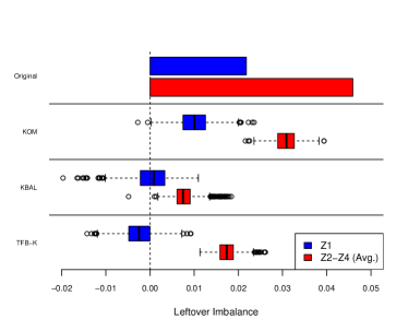
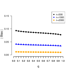
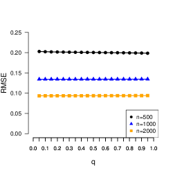
B.6 Performance of TFB-K in DGP 2 across different values of
Figure 20 reports the performance of TFB-K in DGP 2 across varying . At every sample size, TFB-K’s bias and RMSE are stable across all values of tried.
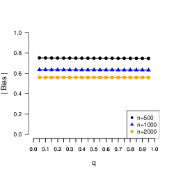
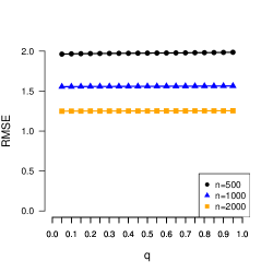
Appendix C Proofs
C.1 Proof of Theorem 1
can be written as the sum of three terms that I analyze separately:
| (71) |
For , first notice that
| (72) |
where Assumption 1 allows the second line in (C.1) above. Therefore,
| (73) |
Thus, the Central Limit Theorem applies to by (C.1) and iid data, meaning that
| (74) |
where by condition (iv) for the theorem. Some manipulation then gives that
| (75) |
Moving to , I first consider its distribution given and . To begin, under Assumption 1, iid data, and condition (i) for the theorem,
| (76) |
Additionally, under conditions (iii) and (v) for the theorem, such that
| (77) |
To see this, Assumption 1, iid data, and conditions (i) and (iii) give
| (78) |
Then, by condition (v) for the theorem, that allow (C.1) to continue as
| (79) |
Therefore, satisfies the Lyapunov condition conditional on and , meaning that, by the Lindberg-Feller theorem,
| (80) |
which also implies here that
| (81) |
or, after some manipulation, that
| (82) |
where by condition (ii).
Putting these pieces together, and are asymptotically independent because they are independent given and and (80) holds given and . Therefore, by (71), (75), and (82)
| (83) |
Further, by condition (vi) for the theorem. Thus, (C.1) can be rewritten as
| (84) |
Finally, examining , it is then evident that
| (85) |
C.2 Proof of Theorem 2
can be rewritten as:
| (86) |
I prove the theorem by showing that and that .
Starting with ,
| (87) |
Given iid data, and thus by the Law of Large Numbers,
| (88) |
where by condition (iv) for Theorem 1. By condition (vii) of the theorem,
| (89) |
and, by the Cauchy-Schwartz Inequality, along with (88) and (89),
| (90) |
Then, under the conditions for Theorem 1, , so
| (91) |
and, by iid data, and thus by the Law of Large Numbers,
| (92) |
| (93) |
Therefore, applying (88), (89), (90), (91), (92), and (93) to (C.2) yields
| (94) |
Moving to in (C.2),
| (95) |
By condition (viii) for the theorem,
| (96) |
Then, by condition (ix) for the theorem,
| (97) |
and using the Cauchy-Schwartz Inequality and (96),
| (98) |
Then, because is finite by condition (ii) for Theorem 1, we find that in (C.2) is . Additionally using (97) allows (C.2) to continue as
| (99) |
Therefore, applying (96), (97), and (99) to (C.2) gives
| (100) |
Finally, applying (94) and (100) to (C.2) completes the proof.
C.3 Proof of Theorem 5
can be written as the sum of four terms that I analyze separately:
| (101) |
For , first notice that
| (102) |
Therefore,
| (103) |
Thus, the Central Limit Theorem applies to by (C.3) and iid data, meaning that
| (104) |
where by condition (iv) for the theorem.
As for and , I only thoroughly derive the asymptotic distribution of , because that of comes from a similar argument. I begin by considering the distribution of given and . Notice that under Assumption 1, iid data, and condition (i) for the theorem,
| (105) |
Additionally, under conditions (iii) and (v) for the theorem, such that
| (106) |
To see this, Assumption 1, iid data, and conditions (i) and (iii) give
| (107) |
Then, by condition (v) for the theorem, that allow (C.3) to continue as
| (108) |
Therefore, satisfies the Lyapunov condition conditional on and , meaning that, by the Lindberg-Feller theorem,
| (109) |
which also implies here that
| (110) |
or, after some manipulation, that
| (111) |
where by condition (ii).
Moving to , the steps to derive its asymptotic distribution are nearly identical to those for , so I omit them here and simply state the final results. One finds that
| (112) |
which also means that
| (113) |
and, after some manipulation, that
| (114) |
where by condition (ii).
Putting these pieces together, , , and are asymptotically independent because they are independent given and and (109) and (112) both hold given and . Therefore, by (C.3), (104), (111), and (114)
| (115) |
Further, by condition (vi) for the theorem. Thus, (C.3) can be rewritten as
| (116) |
Finally, examining , it is then evident that
| (117) |
C.4 Proof of Theorem 6
can be rewritten as:
| (118) |
I prove the theorem by showing that , , and .
Starting with ,
| (119) |
Given iid data, and thus by the Law of Large Numbers,
| (120) |
where is finite by condition (iv) for Theorem 5. By condition (vii) of the theorem,
| (121) |
| (122) |
and, by the Cauchy-Schwartz Inequality, along with (120), (121), and (122)
| (123) |
| (124) |
Then, under the conditions for Theorem 5, , so
| (125) |
and, by iid data, and thus by the Law of Large Numbers,
| (126) |
| (127) |
Therefore, applying (120), (121), (122), (C.4), (124), (125), (126), and (127) to (C.4) yields
| (128) |
Moving to in (C.4),
| (129) |
By condition (viii) for the theorem,
| (130) |
Then, by condition (ix) for the theorem,
| (131) |
and using the Cauchy-Schwartz Inequality and (130),
| (132) |
Then, because is finite by condition (ii) for Theorem 5, we find that in (C.4) is . Additionally using (131) allows (C.4) to continue as
| (133) |
Therefore, applying (130), (131), and (133) to (C.4) gives
| (134) |
As for , deriving its probability limit follows nearly identical steps as does deriving the probability limit of . Therefore, I omit the derivation for and simply state the result. One finds that
| (135) |