Adaptive and Cascaded Compressive Sensing

Abstract

Scene-dependent adaptive compressive sensing (CS) has been a long pursuing goal which has huge potential in significantly improving the performance of CS. However, without accessing to the ground truth image, how to design the scene-dependent adaptive strategy is still an open-problem and the improvement in sampling efficiency is still quite limited. In this paper, a restricted isometry property (RIP) condition based error clamping is proposed, which could directly predict the reconstruction error, i.e. the difference between the currently-stage reconstructed image and the ground truth image, and adaptively allocate samples to different regions at the successive sampling stage. Furthermore, we propose a cascaded feature fusion reconstruction network that could efficiently utilize the information derived from different adaptive sampling stages. The effectiveness of the proposed adaptive and cascaded CS method is demonstrated with extensive quantitative and qualitative results, compared with the state-of-the-art CS algorithms.

1 Introduction

Compressive sensing (CS) has attracted wide attention since it was first proposed in 2006 [10], for it can greatly reduce the sampling rate required for accurate reconstruction. Thus, CS has been applied in many fields, including but not limited to image acquisition [11, 26], accelerated magnetic resonance imaging (MRI) [20] and wireless broadcast [17], etc.

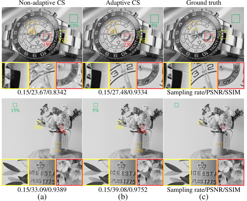
Figure 1: The non-adaptive CS method ISTA-Net+ [37] adopts the same sampling rate for each region of the target scene, which is redundant for some regions, but not enough for other regions. The proposed adaptive CS method can adaptively adjust the sampling rate of different regions according to the characteristics of the target scene, so as to improve the image reconstruction quantity. The percentage number of different colors in the figure represents the sampling rate of the corresponding framed region.

Traditionally, the CS problem can be formulated as

$$\arg\min_{x\in\mathbb{R}^{n}}\|\Psi x\|_{1}\quad\textnormal{s.t. }\Phi x+\epsilon=y,$$ (1)

where $\Phi\in R^{m\times n}$ is the compressive measurement matrix. $\epsilon\in R^{m}$ and $y\in R^{m}$ denote the measurement noise and the compressive measurement. The number of measurements $m$ is commonly much smaller than $n$ and $\Psi$ denotes the sparse transform operator. In this model, the sampling matrix is fixed and predefined, with spatially uniform sampling rate for the entire image. However, depending on the image content, different image regions could be of different complexities, requiring quite different sampling rates for similar reconstruction quality. As shown in Fig. 1, the original image patch can be well recovered at a very low sampling rate for the smooth regions such as the wall and the background. However, a higher sampling rate is required for the regions with more complex textures, such as the pointer of the dial or words on the vase. Therefore, scene-dependent adaptive sampling is quite-promising in achieving much higher sampling efficiency than traditional CS methods.

Adaptive CS has been a long pursuing goal for efficient and adaptive information sampling. The most challenging part in adaptive CS is how to design the adaptive strategy when the ground truth image is not accessible. Previous methods [25, 29, 24] propose to focus on sampling regions with high feature density, according to the intermediate restored image from existing measurements. However, these methods are to-some-extent heuristic and the improvement in CS efficiency are still limited.

In this paper, enlightened by the restricted isometry property (RIP) in CS theory, we propose an efficient adaptive and cascaded CS neural network (ACCSNet).

By utilizing the RIP-condition based clamping on the preceding measurement error maps, the unknown reconstruction errors can be revealed by the known measurement errors. Then, the error-guided adaptive scheme is proposed to realize the adaptive sampling. A cascaded reconstruction network is proposed to collaborate with the multi-stage adaptive sampling strategy. With the stage-to-stage feature fusion mechanism, information among stages can be fully fused and exploited, further improving the quality of reconstruction results. Through comparison with the state-of-the-art CS algorithms, we demonstrate the effectiveness of the proposed method both quantitatively and qualitatively.

In all, the contributions of the proposed method are concluded as below.

• We propose ACCSNet to implement adaptive compressive sampling based on the RIP property in CS theory, which enables to locate and adaptively sample image regions with high reconstruction errors and realize CS imaging with high-efficiency.

• We propose a cascaded information fusion method in the CS reconstruction neural network which could facilitate sufficient information exploration among different stages of adaptive CS and further improve the CS reconstruction quality.

• The effectiveness of the proposed method is extensively demonstrated through comparing with state-of-the-art methods and ablation study.

2 Related Work

From conventional optimization methods [7, 4] to deep-learning based reconstruction methods [33, 37, 23, 16, 32, 34, 6, 27], the performance in CS imaging have been significantly improved. Most of these methods take the samples without considering scene contents, leaving the room for improvement in the performance.

Adaptive Sampling CS imaging

Conventionally, to realize adaptive sampling, compressive measurements are sampled in different stages and the sampling region of the next stage is decided based upon the analysis of the reconstructed results of the previous stages. To decide the sampling region at the next stage, different heuristic methods are proposed to analyze the image characteristic of current-state reconstruction and locate the image region of high density in edges, wavelet coefficients or discrete cosine transform (DCT) coefficients, etc. The adaptive sampling scheme based on wavelet transform [1, 35, 28, 25, 29] adopts cascaded sampling and reconstruction method, which starts from the lowest resolution and obtains a higher resolution image after each stage of sampling and reconstruction. The sampling of each stage is based on the wavelet transform coefficients of the previous low resolution reconstruction results. With these adaptive strategies, the regions with large wavelet coefficients are sampled, and the regions with small wavelet transform coefficients are often discarded. Similar ideas are also applied to other transform domains, e.g. DCT [19], Fourier transform [14]. However, since regions with fine textures can often be neglected in the case of low resolution or low quality, incorporating only the feature characteristics of the intermediate reconstruction to guide the adaptive sampling process is inaccurate and prevents CS imaging of complex images with high accuracy. Recently, inspired by the animal visual mechanism, Phillips et al. [24] proposed an adaptive foveated single-pixel imaging system, which can adaptively sample with a foveated pattern centered at the position of the moving target in the video streams. However, it is for adaptive video CS, which can not be applied to single image CS.

In all, how to design the scene-dependent adaptive CS imaging method without access to the ground truth image is still an open problem, and the potential of the scene-dependent information is still not well-explored with existing adaptive methods. In this paper, we propose an adaptive CS method for single image CS imaging. Through fully exploiting the RIP theory, we propose an adaptive CS imaging method that could directly locate the image regions with high reconstruction error, leading to highly efficient adaptive CS imaging.

Cascaded Compressive Reconstruction

Cascaded CS reconstruction methods propose to reconstruct images of different sampling rates with the same network, which greatly increase the scalability of the imaging system. Xu et al. [32] proposed a multi-stage Laplacian pyramid reconstructive adversarial network named LAPRAN, which can generate images of different resolutions following the concept of Laplacian pyramids. Shi et al. [27] proposed an end-to-end cascaded structure for simultaneously training the sampling matrix and reconstruction network. With the scalable structure and greedy method, multiple sampling rates can be realized with only one network with high quality. However, these multi-stage methods do not take the full advantage of the information among stages, only the sampling results [32] or the reconstruction results [27] are fused between adjacent stages, and all the feature maps generated by the different stages are discarded. In this paper, we propose a cascade information fusion method that could enforce sufficient information fusion among different adaptive stages and further improve the efficiency of adaptive CS imaging.

3 Adaptive and Cascaded CS Net

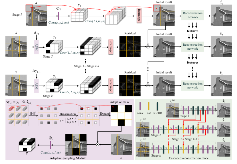
Figure 2: The diagram of k-stage ACCSNet.

Different from the traditional CS model in Eq. 1, we propose to model the CS problem with an multi-stage adaptive and cascaded model,

$$y_{i} =\Phi_{i}x+\epsilon$$ (2)

$$\hat{x_{i}} =\mathcal{N}_{i}(y_{1},y_{2},...,y_{i})$$

$$\Phi_{i+1} =\mathcal{H}(\Delta{y_{i}}),$$

where $x$ is the latent image, $y_{i}$ is the measurement vector of i-th stage, $\Phi_{i}$ is the corresponding sampling matrix, $\mathcal{N}_{i}(\cdot)$ indicates the reconstruction mapping function of i-th stage and is implemented by the cascaded feature fusion network, $\mathcal{H}(\cdot)$ denotes the adaptive sampling module that is realized by the error-induced adaptive sampling module. Expanding the recursive expression in Eq. 2, all modules of multi-stages combine an entire network named ACCSNet. Fig. 2 shows the structure of the k-stage ACCSNet, which can realize different sampling rates and multi-stage reconstruction within only one model.

As for the sampling matrix $\Phi_{i}$, we use a patch-based learnable scheme. The input image $x$ is divided into several non-overlapping $p\times p\times c$ patches $x^{j}$, where $p$ and $c$ denote spacial size and the number of input channels, respectively. In our paper, only grayscale images are applied for the experiment, so the input channel is set to 1. In practice, we use one learnable convolution layer conv(p, p, 1, m) without bias to implement the sampling model, in which the kernel size is $p\times p$, the stride is also $p$, and the number of output channels is $m$. Assuming that the sampling rate of this patch is $r$, then $m$ can be calculated as $\lfloor rp^{2}\rceil$. $\lfloor.\rceil$ represents the rounding calculation.

Adaptive sampling module (ASM) takes $\Delta y_{i}$ of the stage i as input and outputs a binary adaptive mask to determine which regions should be sampled at the stage i+1, as shown in the bottom left of Fig. 2. Except for the first stage, the sampling model of each stage adaptively adjusts the sampling strategy according to the sampling and reconstruction results of the previous stage. The reconstruction model of each stage will continuously fuse feature maps of the previous stage to make full use of the information sampled before, as shown in the top and the bottom right of Fig. 2. In the following, we will introduce the proposed ACCSNet in detail.

3.1 Error-induced Adaptive Sampling Module

Figure 3: Reconstruction results and absolute error image with sampling rate $=0.05$. (a) reconstruction results, (b) absolute error map, (c) ground truth image in Set11 [16].

The core idea of adaptive sampling is how to choose the next sampling strategy according to the existing information. Fig. 3 shows an intuitive example, one intermediate reconstruction result of Set11 [16] at the stage 1 with sampling rate $r=0.05$, the corresponding reconstruction error map and the ground truth image are present in Fig. 3(a-c) respectively. Obviously, the reconstruction error of this uniformly sampled case is not uniform. Therefore, on the next sampling stage, if we can allocate more samples to the regions with larger error, the entire sampling scheme could be more efficient. In other words, we can achieve better sampling efficiency and thus lead to higher reconstruction quality with the same total sampling rate.

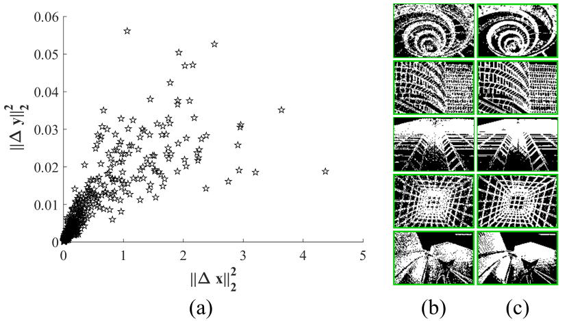
Figure 4: Visual display of the relationship between $||\Delta y||_{2}^{2}$ and $||\Delta x||_{2}^{2}$. (a) statistical diagram of $||\Delta y||_{2}^{2}$ and $||\Delta x||_{2}^{2}$, (b) binary $||\Delta y||_{2}^{2}$, (c) binary $||\Delta x||_{2}^{2}.$

RIP condition based error clamping

The key problem of adaptive sampling is how to estimate the reconstruction error $||\Delta x_{i}||_{2}$ of the stage i without the ground truth image? According to the relationship between the sampling measurements and reconstruction results, we can calculate the measurements error from reconstruction error by

$$\Delta y_{i}=\Phi_{1}\Delta x_{i}=\Phi_{1}(x-\hat{x}_{i})=y_{1}-\Phi_{1}\hat{x}_{i},$$ (3)

where $y_{1}$ and $\Phi_{1}$ are sampling measurements and sampling matrix of stage 1, $\hat{x_{i}}$ denote the reconstruction results of the stage i, and $x$ is the ground truth image, respectively. $\Delta y_{i}$ can be regarded as a sampling measurement of $\Delta x_{i}$. Therefore, the problem becomes how to estimate $||\Delta x_{i}||_{2}$ from the known $||\Delta y_{i}||_{2}$, which is an ill-posed problem. Thanks to the restricted isometry property(RIP) proposed in [5], if the sampling matrix $\Phi_{1}$ satisfies the RIP which is the basic premise of CS, the reconstruction errors could be campled by the measurement errors with the inequality

$$\frac{||\Delta y||_{2}^{2}}{(1+\delta)}\leq||\Delta x||_{2}^{2}\leq\frac{||\Delta y||_{2}^{2}}{(1-\delta)},$$ (4)

where $\delta\in(0,1)$. RIP provides a double side clamping for the $l_{2}$ norm of the reconstruction errors $\Delta x$. Therefore, it is reasonable to conclude that if the measurement error $||\Delta y||_{2}^{2}$ is relatively large, the corresponding reconstruction error $||\Delta x||_{2}^{2}$ is probably large as well, and vice versa.

Here, we verify the effectiveness of estimating $||\Delta x||_{2}^{2}$ from $||\Delta y||_{2}^{2}$ according to the statistical results and comparison of the quantized adaptive masks. From the statistical results shown in Fig. 4(a), $||\Delta y||_{2}^{2}$ and $||\Delta x||_{2}^{2}$ have a nearly linear relationship. We also calculate the adaptive masks according to $||\Delta x||_{2}^{2}$ and $||\Delta y||_{2}^{2}$, and demonstrate the results in Fig. 4(b) and (c) respectively. Each element of the binarization mask corresponds to a region, with first $\alpha$ ($\alpha=70\%$ in this paper) larger $||\Delta y||_{2}^{2}$ as 1 and the rest as 0. It can be seen that the adaptive masks calculated according to $||\Delta x||_{2}^{2}$ and $||\Delta y||_{2}^{2}$ are highly consistent. To sum up, by calculating $||\Delta y||_{2}^{2}$, we can get which regions have larger reconstruction errors, which provides a basis for the next sampling.

Error based adaptive strategy

The lower left corner of Fig. 2 shows the schematic diagram of the adaptive sampling module. The error based adaptive strategy determines which image patches should be sampled at the stage i according to the measurement error of the stage i-1 of each image patch. Except for the stage 1, according to the adaptive mask calculated by the adaptive sampling module, the ACCSNet only samples the regions with relatively poor reconstruction quality of the previous stage. Through this adaptive and cascaded sampling mechanism, different regions of an image are sampled with different sampling rates efficiently. The details of Error based adaptive strategy are concluded in Alg. 1.

Algorithm 1 Error based adaptive strategy

0:  Sampling scale factor $\alpha$, patch size $p$, samping measurement $y_{1}$ and sampling matrix $\Phi_{1}$ of the stage 1, reconstruction result $\hat{x}_{i-1}$ of the stage i+1, ground truth image $x$ with scale $H\times W$

0:  Sampling measurement $y_{i}$ of the stage i

1:  Calculate the measurement error: $\Delta y_{i-1}=y_{1}-\Phi_{1}\hat{x}_{i-1}$

2:  Calculate the $l_{2}$ norm of each patch j: $V=[\|\Delta y_{i-1}^{1}\|_{2}^{2},\|\Delta y_{i-1}^{2}\|_{2}^{2},...,\|\Delta y_{i-1}^{j}\|_{2}^{2}]$

3:  Calculate the number of patches not sampled of the stage i: $N_{a}=(1-\alpha^{i-1})\times\frac{H}{p}\times\frac{W}{p}$

4:  Sort $V$ from small to large: $V_{\mathrm{sorted}}=\mathrm{sort}_{\uparrow}(V)$

5:  Find the $N_{a}-th$ smallest value of V as the threshold $T$ of binarization: $T=V_{\mathrm{sorted}}(N_{a})$

6:  Binarize V based on $T$:

$$B_{a}=\left\{\begin{array}[]{rcl}1&{V>T}\\ 0&{V\leq T}\end{array}\right.$$

7:  Expand $B_{a}$ to generate a pixel-wise adaptive mask $E_{a}$

8:  Sample patches based on the adaptive mask $E_{a}$: $y_{i}=\Phi_{i}(E_{a}\odot x)$

9:  return $y_{i}$

3.2 Cascaded Feature Fusion Network Structure

As shown in Fig. 2, the reconstruction model of each stage contains an initial linear layer and a reconstruction network. The initial linear layer of the stage 1 is a linear transformation, which maps the sampling results of $m_{i}$ channels to $p^{2}c$ channels through only one $1\times 1$ convolution layer, and then obtains the initial reconstruction result of the same size as the input image through rearrange operation. The rearrange operation includes a reshape layer and a concatenate layer. Specifically, reshape the one-dimensional reconstruction result of each image patch with the length of $p^{2}c$ into a three-dimensional image patch with the dimension of $p\times p\times c$, and then concatenate them into the original dimension of the image in the spatial dimension. The initial reconstruction network of stage 2 or later stages have the same $1\times 1$ convolution layer with stage 1, but different parameters. Also, there is an addition layer after the convolution layer, through the addition layer, the output of the $1\times 1$ convolution layer is added to the initial reconstruction result of the previous stage to obtain the initial reconstruction result of the current stage. Because of the design of the addition layer, the goal of the later stage is to reconstruct the residual between the previous stage initial reconstruction result and the ground truth image.

The reconstruction network of the stage 1 adopts a symmetrical hourglass network with residual learning [12], which contains four convolution layers (two at both ends) and three RRDBs [30] (in the middle). All these convolution layers are followed by the LeakyRelu [31] nonlinear activation function. The reconstruction network of the stage 2 and the later stages take the initial reconstruction result of the current stage as input, and fuse the feature maps from the previous stage to output the final reconstruction result of the current stage. The reconstruction network of stage i (i $>$ 1) is similar to the deep reconstruction network of stage 1, but the former has three more convolution layers and three concatenate layers than the latter as shown in the lower right corner of Fig. 2.

3.3 Loss Function and Training Strategy

For network training, we adopt $l_{1}$ loss to supervise the initial reconstruction result and the final reconstruction result for each stage. Given input image $x$, the learnable sampling matrix $\Phi_{i}$, the samping measurements of the stage i can be denoted as $\mathcal{F}_{\Phi_{i}}(x)$. Therefore, for the i-th stage, the loss function can be expressed as:

$$\mathcal{L}_{i} =\mathcal{L}_{i}^{\mathrm{final}}+\beta\ \mathcal{L}_{i}^{\mathrm{init}}$$

$$=\|\mathcal{N}_{i}^{\mathrm{final}}(\mathcal{F}_{\Phi_{i}}(x))-x\|_{1}+\beta\|\mathcal{N}_{i}^{\mathrm{init}}(\mathcal{F}_{\Phi_{i}}(x))-x\|_{1},$$

where $\beta$, $\mathcal{N}^{\mathrm{final}}_{i}(.)$ and $\mathcal{N}^{\mathrm{init}}_{i}(.)$ denotes the loss balance hyper-parameter, the full reconstruction network and the initial reconstruction network respectively. We train the k-stage model gradually, which means we fix the parameters of the previous stage after we complete the training process of the previous stage and then train the next stage until we complete the training of the whole model.

4 Experiments

4.1 Dataset and implementation details

We use 200 images from BSDS500 trainset [2] and 91 images from [8] to train our model, and the validation set from BSDS500 is used for validation. Set5 [3], Set11 [16], Set14 [36], BSD68 [21], the testsets from BSDS500, General100 [9], Urban100 [13] and Manga109 [22] are used for testing. For the experiments, the Y channel of the images in YUV color space are utilized. We randomly crop $128\times 128$ image patches from the training dataset during the training process. Batchsize is set as $2$. $\beta$ is chosen empirically as $1$. In Sec. 4.2 and Sec. 4.3, we set the image patch size $p$ and sampling scale factor $\alpha$ to 8 and 0.7, respectively. Adam optimizer [15] is adopted with $\beta_{1}=0.9$, $\beta_{2}=0.999$ and $\epsilon=1\times 10^{-8}$. We set the number of CS reconstruction stages to 4 and sampling rate to 0.05 for each stage. The proposed adaptive sampling strategy is introduce at stage 2 to 4. We train 500k iterations at each stage, the initial learning rate is set to $2\times 10^{-4}$, and multiplied by $0.5$ every other 100k iterations. All the experiments are implemented on the PyTorch platform with a NVIDIA RTX 3090 GPU.

4.2 Comparison with state-of-the-art CS algorithms

Table 1: Performance comparison with state-of-the-art CS algorithms on Set11 [16], BSDS500 testset [2], Urban100 [13], General100 [9] and Manga109 [22]. The best performance is highlighted in red (1st best) and blue (2nd best).

Datasets	Rate	ReconNet  [16]		LAPRAN  [32]		ISTA-Net+  [37]		SCSNet  [27]		MAC-Net  [6]		Ours
		PSNR	SSIM	PSNR	SSIM	PSNR	SSIM	PSNR	SSIM	PSNR	SSIM	PSNR	SSIM
Set11	0.05	22.24	0.6352	21.58	0.5913	22.70	0.6661	24.65	0.7290	22.77	0.7067	26.61	0.8162
	0.1	24.80	0.7284	23.78	0.6893	26.53	0.7992	28.16	0.8506	25.91	0.8042	29.76	0.8847
	0.15	25.55	0.7733	24.27	0.6897	28.67	0.8541	29.75	0.8875	27.56	0.8478	31.86	0.9139
	0.2	27.39	0.8110	26.04	0.7727	30.56	0.8900	31.30	0.9132	29.08	0.8797	33.61	0.9309
BSDS500	0.05	24.07	0.6189	23.58	0.5812	24.18	0.6289	26.77	0.6972	23.77	0.6489	26.72	0.7310
	0.1	25.79	0.6881	25.11	0.6517	26.50	0.7306	28.57	0.7844	25.97	0.7341	29.33	0.8292
	0.15	26.39	0.7337	25.38	0.6500	28.10	0.7874	29.79	0.8509	27.06	0.7800	31.11	0.8713
	0.2	27.63	0.7665	26.77	0.7271	29.38	0.8295	31.10	0.8731	28.35	0.8210	32.67	0.8976
Urban100	0.05	21.36	0.5761	20.85	0.5331	21.89	0.6117	23.28	0.6514	21.56	0.6347	24.89	0.7444
	0.1	23.31	0.6622	22.51	0.6171	24.87	0.7392	26.03	0.7873	24.23	0.7404	27.80	0.8422
	0.15	24.18	0.7146	23.03	0.6294	26.88	0.8054	27.36	0.8348	25.54	0.7896	29.62	0.8793
	0.2	25.47	0.7535	24.28	0.7027	28.35	0.8499	28.60	0.8700	27.01	0.8326	31.08	0.9009
General100	0.05	25.28	0.6990	24.66	0.6600	26.11	0.7182	28.06	0.7702	26.42	0.7482	30.07	0.8308
	0.1	27.91	0.7702	26.81	0.7333	29.82	0.8218	31.88	0.8754	29.54	0.8276	33.54	0.9013
	0.15	27.90	0.8094	26.91	0.7254	31.95	0.8683	33.63	0.9107	31.18	0.8658	35.64	0.9267
	0.2	29.91	0.8375	29.07	0.8047	33.66	0.8996	35.23	0.9341	32.93	0.8968	37.23	0.9418
Manga109	0.05	23.04	0.7025	22.24	0.6570	24.17	0.7518	25.10	0.7520	23.77	0.7786	28.26	0.8731
	0.1	25.96	0.7830	24.64	0.7418	28.84	0.8675	30.17	0.8968	27.67	0.8675	33.27	0.9384
	0.15	26.65	0.8254	25.14	0.7414	31.69	0.9099	32.36	0.9292	29.83	0.9039	36.45	0.9567
	0.2	28.96	0.8553	27.33	0.8199	33.90	0.9347	34.48	0.9508	31.92	0.9294	38.70	0.9652

In this section, we compare with other CS algorithms proposed in recent years, i.e. ReconNet [16], LAPRAN [32], ISTA-Net+ [37], SCSNet [27] and MAC-Net [6]. For comparison, we use the code provided by the author and the settings of training and testing are chosen according to the original paper. The quantitative results comparison is shown in Tab. 1. It can be seen that the reconstruction performance of the proposed adaptive CS algorithm are largely improved than the existing CS algorithms in both PSNR and SSIM, especially at the sampling rates of 0.1, 0.15 and 0.2, when the ASM is introduced.

Fig. 5 shows the reconstruction results with the sampling rates of 0.1, 0.15 and 0.2 respectively. It can be seen that at a sampling rate of 0.1, our method can reconstruct the head of the parrot more accurately, with much higher visual quality. With the proposed ASM, different sampling rates are allocated for different regions according to the reconstruction error of different regions. During the adaptive sampling process, since the reconstruction error of the head area is high, the sampling rate of that region is then adaptively increased and thus enables to achieve better reconstruction results at the same sampling rates. The same comparison results are shown at the lizard and night scene at the sampling rates of 0.15 and 0.2 respectively in Fig. 5. As are shown, the reconstruction accuracy of the structures on the head of the lizard and the appearance of the house are largely improved, with the same overall CS sampling rates with the other methods.

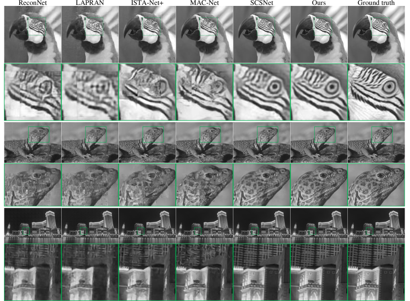
Figure 5: Visual comparison with the state-of-the-art CS algorithms. Top rows: Parrots from Set11 [16] with sampling rate = 0.1, middle rows: 41096 from BSDS500 testset [2] with sampling rate = 0.15, bottom rows: img_085 from Urban100 [13] with sampling rate = 0.2.

4.3 Ablation study

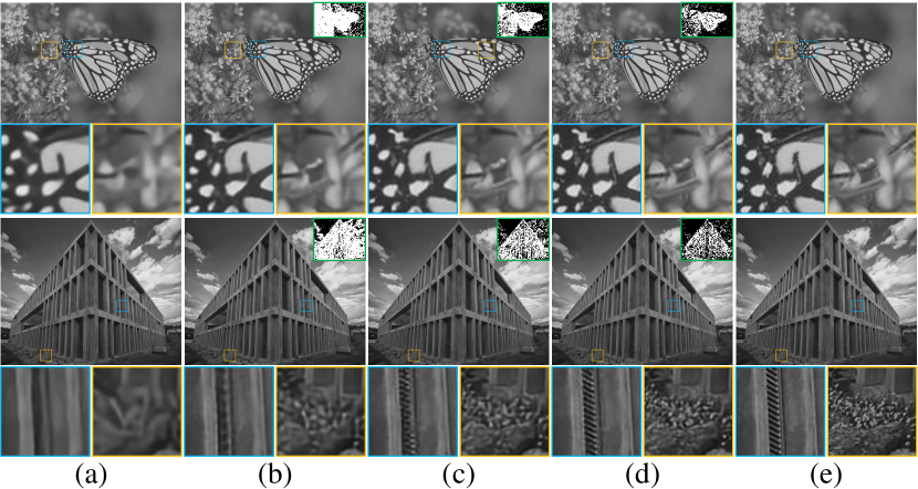
Figure 6: Reconstruction results of four stages, the corresponding adaptive mask is displayed in the top right of the image, which is narrowed and framed with a green box. (a) Stage 1, sampling rate = 0.05, (b) stage 2, sampling rate = 0.1, (c) stage 3, sampling rate = 0.15, (d) stage 4, sampling rate = 0.2, (e) ground truth.

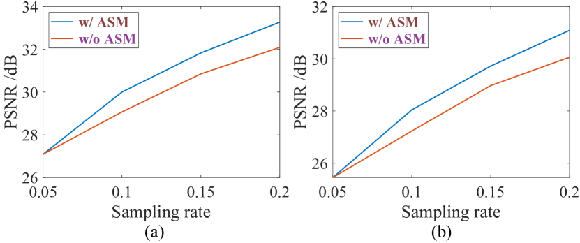
Figure 7: Ablation study of ASM on (a) Set14 [36], (b) BSD68 [21]. w/o and w/ denote without and with respectively.

Figure 8: Ablation study of ASM with sampling rate = 0.1 on test040 (1st and 2nd row) from BSD68 [21] and sampling rate = 0.15 on PPT3 (3rd and 4th row) from Set14 [36]. The adaptive masks generated by ASM are placed in the upper left corner of the images of the 2nd column and framed with a green box. (a) Without ASM, (b) with ASM, (c) ground truth.

Effectiveness of ASM

Fig. 6 shows the reconstruction results of different stages and the corresponding binary adaptive masks. The binary adaptive masks adaptively focus on the regions with more reconstruction errors, and the reconstruction results are gradually improved. We implement an ablation study to verify the effectiveness of the proposed ASM. Fig. 7 shows the PSNR of our algorithm in the reconstruction results with the ASM and without the ASM. Except for stage 1, the proposed ASM can bring about 1dB improvement in PSNR. From the visual reconstruction results shown in Fig. 8, the model with the ASM can reconstruct more accurate image details, while there are serious artifacts in the reconstruction results without the ASM at the same overall sampling rate.

Table 2: Quantitative reconstruction results with and without feature fusion on Set5 [3] and BSDS500 testset [2].

Datasets	Rate	w/o feature fusion		w/ feature fusion
		PSNR	SSIM	PSNR	SSIM
Set5	0.05	30.01	0.8602	30.01	0.8602
	0.1	33.95	0.9210	34.04	0.9216
	0.15	35.58	0.9354	35.89	0.9380
	0.2	36.70	0.9438	37.19	0.9477
BSDS500	0.05	26.72	0.7310	26.72	0.7310
	0.1	29.25	0.8276	29.33	0.8292
	0.15	30.90	0.8693	31.11	0.8713
	0.2	32.28	0.8920	32.67	0.8976

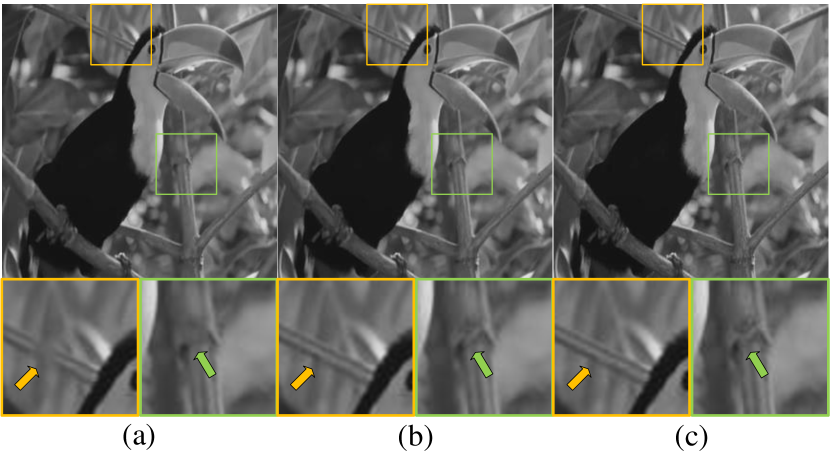
Figure 9: Ablation study of feature fusion on bird from Set5 [3] with sampling rate = 0.15. (a) Without feature fusion, (b) with feature fusion, (c) ground truth.

Effectiveness of feature fusion

We propose cascaded feature-fusion connections between different stages to fuse the features of the previous stage into the reconstruction network of the current stage and assist the proposed ASM in highly-efficient image reconstruction. Tab. 2 shows the quantitative results with and without feature fusion connections between stages. Note that the improvement with cascaded feature fusion starts from stage 2, the improvement of introducing the cascaded feature fusion starts from stage 2. From comparison results, we can see that the quantitative results of the reconstruction results of our method with cascaded feature fusion are better than those without cascaded feature fusion among stages. Fig. 9 shows the visual reconstruction results of different models. The model with cascaded feature fusion can reconstruct elegantly higher quality and better visual results. As compared, the cascaded feature fusion enables the information of the previous stage to be transmitted to the later stage, and can make full use of the information among stages for further reconstruction quality improvement.

4.4 Exploration of model hyper-parameters

Table 3: Quantitative results with different patch sizes on Set14 [36] and General100 [9].

Datasets	Rate	patch size = 8		patch size = 16		patch size = 32
		PSNR	SSIM	PSNR	SSIM	PSNR	SSIM
Set14	0.05*	27.09	0.7467	27.30	0.7525	27.16	0.7449
	0.1	30.00	0.8343	29.99	0.8331	29.84	0.8257
	0.15	31.83	0.8700	31.86	0.8676	31.28	0.8609
	0.2	33.27	0.8918	32.76	0.8861	32.35	0.8805
General100	0.05*	29.81	0.8261	30.08	0.8315	29.94	0.8251
	0.1	33.54	0.9013	33.44	0.8977	33.21	0.8917
	0.15	35.64	0.9267	35.52	0.9238	34.76	0.9172
	0.2	37.23	0.9418	36.52	0.9371	35.93	0.9319

• When the sampling rate is 0.05, one of the main reasons for the difference of reconstruction results is the error introduced when calculating the number of corresponding sampling points by rounding method. For example, when the patch size is 8, the number of sampling points of each patch should be calculated as $\lfloor 0.05\times 8^{2}\rceil=3$, and the corresponding real sampling rate should be $3/64=0.0469$. Similarly, when the patch size is 16, the corresponding real sampling rate should be 0.0508.

Exploration of different image patch size

The sampling model proposed in this paper divides the image into non-overlapping small patches and samples different patches respectively. In the sampling model of stage 2 and later stages, the adaptive module determines whether different patches need to be sampled or not. If the image is divided with smaller patch size, the proposed ASM can determine the adaptive sampling distribution with finer scale, which could help to reconstruct the whole image with higher quality. In order to choose a proper patch size, we conduct the patch-size analysis experiments and the quantitative results are concluded in Tab. 3. As shown, the overall performance at patch size 8, 16, 32 are slightly different and the difference increases as the sampling rate increases. According to the quantitative comparison results, we choose 8 as the patch size in our experiments.

Table 4: Average quantitative results of different sampling rates at different sampling scale factors $\alpha$ on Set5  [36] and BSDS500  [9].

Datasets	$\alpha$ = 0.5	$\alpha$ = 0.6	$\alpha$ = 0.7	$\alpha$ = 0.8
	PSNR/SSIM	PSNR/SSIM	PSNR/SSIM	PSNR/SSIM
Set5	34.20/0.9144	34.27/0.9164	34.28/0.9169	34.08/0.9164
BSDS500	30.01/0.8275	30.02/0.8310	30.02/0.8323	29.72/0.8307

Exploration of sampling scale factor $\alpha$

Different sampling scale factors $\alpha$ will affect the proportion of 1 in the adaptive mask, that is, the number of sampling regions of each adaptive sampling stage. A larger sampling scale factor $\alpha$ can allocate more regions of the image at each adaptive stage, but for a fixed overall sampling rate, the number of adaptive sampling stages will be reduced. With reduced adaptive stage number, the resolution of sampling rate will be reduced, limiting the potential of adaptive sampling. On the other hand, if the sampling scale factor $\alpha$ is too small, the number of adaptive stages is too big and the speed of the adaptive imaging will be slow. In order to choose a proper sampling factor, we conduct parameter analysis upon $\alpha$. The quantitative results are shown in Tab. 4, with $\alpha$ ranging from 0.5 to 0.8. As is shown, when $\alpha$ increases from 0.5 to 0.7, the overall performance gradually increases. However, when we increase $\alpha$ from $0.7$ to $0.8$, the reconstructed quality starts to decrease. Therefore, according to our experimental results, we choose $\alpha=0.7$ to obtain the best performance in our experiments.

5 Discussion

In this paper, we propose an adaptive compressive sensing method which could adaptively adjust the sampling region among stages and realize state-of-the art performance. Since the adaptive sampling module requires the reconstruction results of the previous stage as one of the inputs, the inferencing of the reconstruction neural network will be the bottleneck in the real-time CS imaging. However, we need to note that the main contribution of the proposed method in this paper is to develop an highly-efficient adaptive CS imaging principle, based upon the RIP condition theory, and we believe that through adopting techniques such as network compression, quantization, or pruning [18], the inferencing speed could be greatly accelerated and the proposed method could be readily applied for real-time adaptive CS imaging. We will leave the network acceleration of the proposed method as further work.

6 Conclusion

In conclusion, we propose an adaptive and cascaded CS method, which can adaptively sample natural images with scene-dependent information, based on the RIP theory. Cascaded feature fusion between stages are proposed for CS reconstruction, which makes full use of the information among stages and elegantly helps to further improve the reconstruction efficiency. Quantitative and qualitative experiments are conducted and demonstrate the state-of-the-art CS effectiveness of the proposed method.

References

- Amann and Bayer [2013] Marc Amann and Manfred Bayer. Compressive adaptive computational ghost imaging. Scientific reports, 3(1):1–5, 2013.
- Arbelaez et al. [2010] Pablo Arbelaez, Michael Maire, Charless Fowlkes, and Jitendra Malik. Contour detection and hierarchical image segmentation. IEEE transactions on pattern analysis and machine intelligence, 33(5):898–916, 2010.
- Bevilacqua et al. [2012] Marco Bevilacqua, Aline Roumy, Christine Guillemot, and Marie Line Alberi-Morel. Low-complexity single-image super-resolution based on nonnegative neighbor embedding. 2012.
- Boyd et al. [2011] Stephen Boyd, Neal Parikh, and Eric Chu. Distributed optimization and statistical learning via the alternating direction method of multipliers. Now Publishers Inc, 2011.
- Candes [2008] Emmanuel J Candes. The restricted isometry property and its implications for compressed sensing. Comptes rendus mathematique, 346(9-10):589–592, 2008.
- Chen et al. [2020] Jiwei Chen, Yubao Sun, Qingshan Liu, and Rui Huang. Learning memory augmented cascading network for compressed sensing of images. In Proceedings of the European Conference on Computer Vision, pages 513–529, 2020.
- Daubechies et al. [2004] Ingrid Daubechies, Michel Defrise, and Christine De Mol. An iterative thresholding algorithm for linear inverse problems with a sparsity constraint. Communications on Pure and Applied Mathematics, 57(11):1413–1457, 2004.
- Dong et al. [2014] Chao Dong, Chen Change Loy, Kaiming He, and Xiaoou Tang. Learning a deep convolutional network for image super-resolution. In Proceedings of the European Conference on Computer Vision, pages 184–199, 2014.
- Dong et al. [2016] Chao Dong, Chen Change Loy, and Xiaoou Tang. Accelerating the super-resolution convolutional neural network. In Proceedings of the European Conference on Computer Vision, pages 391–407. Springer, 2016.
- Donoho [2006] David L Donoho. Compressed sensing. IEEE Transactions on information theory, 52(4):1289–1306, 2006.
- Duarte et al. [2008] Marco F Duarte, Mark A Davenport, Dharmpal Takhar, Jason N Laska, Ting Sun, Kevin F Kelly, and Richard G Baraniuk. Single-pixel imaging via compressive sampling. IEEE signal processing magazine, 25(2):83–91, 2008.
- He et al. [2016] Kaiming He, Xiangyu Zhang, Shaoqing Ren, and Jian Sun. Deep residual learning for image recognition. In Proceedings of the IEEE Conference on Computer Vision and Pattern Recognition, pages 770–778, 2016.
- Huang et al. [2015] Jia-Bin Huang, Abhishek Singh, and Narendra Ahuja. Single image super-resolution from transformed self-exemplars. In Proceedings of the IEEE Conference on Computer Vision and Pattern Recognition, pages 5197–5206, 2015.
- Jiang et al. [2017] Hongzhi Jiang, Shuguang Zhu, Huijie Zhao, Bingjie Xu, and Xudong Li. Adaptive regional single-pixel imaging based on the fourier slice theorem. Optics express, 25(13):15118–15130, 2017.
- Kingma and Ba [2014] Diederik P Kingma and Jimmy Ba. Adam: A method for stochastic optimization. arXiv preprint arXiv:1412.6980, 2014.
- Kulkarni et al. [2016] Kuldeep Kulkarni, Suhas Lohit, Pavan Turaga, Ronan Kerviche, and Amit Ashok. Reconnet: Non-iterative reconstruction of images from compressively sensed measurements. In Proceedings of the IEEE Conference on Computer Vision and Pattern Recognition, pages 449–458, 2016.
- Li et al. [2013] Chengbo Li, Hong Jiang, Paul Wilford, Yin Zhang, and Mike Scheutzow. A new compressive video sensing framework for mobile broadcast. IEEE Transactions on Broadcasting, 59(1):197–205, 2013.
- Liang et al. [2021] Tailin Liang, John Glossner, Lei Wang, Shaobo Shi, and Xiaotong Zhang. Pruning and quantization for deep neural network acceleration: A survey. Neurocomputing, 461:370–403, 2021.
- Liu and Ling [2017] Jiying Liu and Cong Ling. Adaptive compressed sensing using intra-scale variable density sampling. IEEE Sensors Journal, 18(2):547–558, 2017.
- Lustig et al. [2007] Michael Lustig, David Donoho, and John M Pauly. Sparse mri: The application of compressed sensing for rapid mr imaging. Magnetic Resonance in Medicine, 58(6):1182–1195, 2007.
- Martin et al. [2001] David Martin, Charless Fowlkes, Doron Tal, and Jitendra Malik. A database of human segmented natural images and its application to evaluating segmentation algorithms and measuring ecological statistics. In Proceedings of the IEEE International Conference on Computer Vision, volume 2, pages 416–423, 2001.
- Matsui et al. [2017] Yusuke Matsui, Kota Ito, Yuji Aramaki, Azuma Fujimoto, Toru Ogawa, Toshihiko Yamasaki, and Kiyoharu Aizawa. Sketch-based manga retrieval using manga109 dataset. Multimedia Tools and Applications, 76(20):21811–21838, 2017.
- Metzler et al. [2017] Christopher A Metzler, Ali Mousavi, and Richard G Baraniuk. Learned d-amp: Principled neural network based compressive image recovery. arXiv preprint arXiv:1704.06625, 2017.
- Phillips et al. [2017] David B Phillips, Ming-Jie Sun, Jonathan M Taylor, Matthew P Edgar, Stephen M Barnett, Graham M Gibson, and Miles J Padgett. Adaptive foveated single-pixel imaging with dynamic supersampling. Science advances, 3(4):e1601782, 2017.
- Rousset et al. [2016] Florian Rousset, Nicolas Ducros, Andrea Farina, Gianluca Valentini, Cosimo D’Andrea, and Françoise Peyrin. Adaptive basis scan by wavelet prediction for single-pixel imaging. IEEE Transactions on Computational Imaging, 3(1):36–46, 2016.
- Sankaranarayanan et al. [2012] Aswin C Sankaranarayanan, Christoph Studer, and Richard G Baraniuk. Cs-muvi: Video compressive sensing for spatial-multiplexing cameras. In IEEE International Conference on Computational Photography, pages 1–10, 2012.
- Shi et al. [2019] Wuzhen Shi, Feng Jiang, Shaohui Liu, and Debin Zhao. Scalable convolutional neural network for image compressed sensing. In Proceedings of the IEEE Conference on Computer Vision and Pattern Recognition, pages 12290–12299, 2019.
- Soldevila et al. [2015] Fernando Soldevila, Eva Salvador-Balaguer, P Clemente, Enrique Tajahuerce, and Jesús Lancis. High-resolution adaptive imaging with a single photodiode. Scientific reports, 5(1):1–9, 2015.
- Wang et al. [2019] Qiong Wang, Qiurong Yan, Suhui Deng, Hui Wang, Chenglong Yuan, and Yuhao Wang. Iterative adaptive photon-counting compressive imaging based on wavelet entropy automatic threshold acquisition. IEEE Photonics Journal, 11(5):1–13, 2019.
- Wang et al. [2018] Xintao Wang, Ke Yu, Shixiang Wu, Jinjin Gu, Yihao Liu, Chao Dong, Yu Qiao, and Chen Change Loy. Esrgan: Enhanced super-resolution generative adversarial networks. In Proceedings of the European conference on computer vision workshops, pages 0–0, 2018.
- Xu et al. [2015] Bing Xu, Naiyan Wang, Tianqi Chen, and Mu Li. Empirical evaluation of rectified activations in convolutional network. arXiv preprint arXiv:1505.00853, 2015.
- Xu et al. [2018] Kai Xu, Zhikang Zhang, and Fengbo Ren. Lapran: A scalable laplacian pyramid reconstructive adversarial network for flexible compressive sensing reconstruction. In Proceedings of the European Conference on Computer Vision, pages 485–500, 2018.
- Yang et al. [2016] Yan Yang, Jian Sun, Huibin Li, and Zongben Xu. Deep admm-net for compressive sensing mri. In Proceedings of the 30th international conference on neural information processing systems, pages 10–18, 2016.
- Yao et al. [2019] Hantao Yao, Feng Dai, Shiliang Zhang, Yongdong Zhang, Qi Tian, and Changsheng Xu. Dr2-net: Deep residual reconstruction network for image compressive sensing. Neurocomputing, 359:483–493, 2019.
- Yu et al. [2014] Wen-Kai Yu, Ming-Fei Li, Xu-Ri Yao, Xue-Feng Liu, Ling-An Wu, and Guang-Jie Zhai. Adaptive compressive ghost imaging based on wavelet trees and sparse representation. Optics express, 22(6):7133–7144, 2014.
- Zeyde et al. [2010] Roman Zeyde, Michael Elad, and Matan Protter. On single image scale-up using sparse-representations. In International conference on curves and surfaces, pages 711–730. Springer, 2010.
- Zhang and Ghanem [2018] Jian Zhang and Bernard Ghanem. Ista-net: Interpretable optimization-inspired deep network for image compressive sensing. In Proceedings of the IEEE Conference on Computer Vision and Pattern Recognition, pages 1828–1837, 2018.