Tripartite entanglement and matrix inversion quantum algorithm
Abstract
The role of entanglement is discussed in the Harrow-Hassidim-Lloyd (HHL) algorithm. We compute all tripartite entanglement at every steps of the HHL algorithm. The tripartite entanglement is generated in the first quantum phase estimation (QPE) step. However, it turns out that amount of the generated entanglement is not maximal except very rare cases. In the second rotation step some tripartite entanglement is annihilated. Thus, the net tripartite entanglement is diminished. At the final inverse-QPE step the matrix inversion task is completed at the price of complete annihilation of the entanglement. An implication of this result is discussed.
I Introduction
In quantum information processing quantum entanglementtext ; schrodinger-35 ; horodecki09 plays an important role as a physical resource. It is used in various quantum information processing, such as quantum teleportationteleportation ; Luo2019 , superdense codingsuperdense , quantum cloningclon , quantum cryptographycryptography ; cryptography2 , quantum metrologymetro17 , and quantum computerqcreview ; computer ; supremacy-1 . Furthermore, quantum computers with hundred qubits were already constructed in IBM and Google. In this reason the development of quantum algorithms becomes important more and more to use the quantum computers efficiently.
The representative of the quantum algorithm are Shor’ factoringshor94 and Grover’s searchgrover96 algorithms. Few years ago another quantum algorithmhhl called Harrow-Hassidim-Lloyd (HHL) algorithm was developed. It is a quantum algorithm, which can compute the inverse of sparse matrix. If is a sparse matrix, HHL algorithm completes the inversion task with a runtime of , where is the maximum number of non-zero entries in row or column, the condition number, and the precision. Since same task can be implemented in the classical computer with a runtime of even though the most efficient algorithm is adopted, one can say that the HHL algorithm improves exponentially in the matrix inversion task over the best classical algorithm. This algorithm is based on the efficient Hamiltonian simulationberry05 . Subsequently, there was a proposals to deal with dense matricesdense . Also a hybrid algorithmhybrid was proposed, where both classical and quantum computers are used appropriately.
In this paper we examine a question: ‘how much the HHL algorithm uses the quantum entanglement efficiently?’. In order to explore this issue we compute the tripartite entanglement in every steps of the HHL algorithm by choosing an experimental realization of the algorithm presented in Ref. exp-hhl-1 . Since the HHL algorithm is known to be optimalhhl in the matrix inversion task and entanglement is known as a physical resource, we expect that much entanglement is created and finally annihilated during the process of the algorithm. However, it turns out that maximal tripartite entanglement is not created except very rare cases. As expected, all created entanglement is annihilated at the final step of the algorithm.
This paper is organized as follows. In Sec. II we discuss the role of entanglement in the Grover’s algorithm. In Sec. III we compute the three-tangleckw of some rank- mixture. The result of this section will be used in Sec. V. In Sec. IV we briefly review the HHL algorithm. In Sec. V we compute the tripartite entanglement at every steps of the HHL algorithm. In Sec. VI a conclusion and further discussion are presented. In appendix A the quantum phase estimation (QPE) is discussed when the unitary operator is operated to the non-eigenvector . The result of this appendix is used in Sec. IV.
II Entanglement in Grover’s algorithm
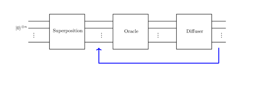
Let us consider a set with . Grover’s algorithmgrover96 ; grover97 is a quantum algorithm, which tries to find a particular quantum state . Grover’s algorithm consists of three unitary transformations called superposition, oracle, and diffuser. The superposition transforms the initial state to a superposed state, where all states in are superposed with equal probability amplitude. This can be achieved by making use of the Hadamard gate
| (3) |
Therefore, after superposition transformation the initial state is changed into
| (4) |
where . The oracle and diffuser are described by the unitary operators and , respectively. The oracle changes a sign of in . The diffuser increases the probability amplitude of from . Given the oracle and diffuser transformations are repeated roughly timesbennett97 ; boyer96 ; grover98 222As proved in Ref. grover98 , the optimal number of queries is when is very large. for large . The schematic quantum circuit of the Grover’s algorithm is plotted in Fig. 1.
The role of entanglement manifestly appears when . If we assume in this case, transforms into
| (5) |
Since the concurrence, one of the bipartite entanglement measure, is defined as for two qubit pure state form2 ; form3 , changes the separable state into the maximally entangled state . Then, exactly detects , which means . Therefore, creates an entanglement maximally and increases the probability amplitude of maximally at the price of complete annihilation of entanglement.
Table I: Entanglement flow in Grover’s algorithm when
Even though Grover’s algorithm is optimal as a quantum searching algorithmzalka99 , such maximal creation and complete annihilation of entanglement do not occur for large . For example, let us consider case. If , Grover’s algorithm changes the quantum state as
| (6) | |||
The three-tangles ckw for and concurrencesform2 ; form3 for the reduced mixed states are summarized in Table I. As Table I shows, transforms the separable state to , whose three-tangle is . Since maximum three-tangle is 333Maximal three-tangle is realized in the Greenberger-Horne-Zeilinger (GHZ) statedur00-1 and its local unitary transformed states., is only partially entangled state. Thus, maximal entanglement creation does not occur in this case. changes into , whose three-tangle is . Therefore, the complete annihilation of tripartite entanglement also does not occur. Same is true for and . Similar behavior occurs in the bipartite entanglement.
III three-tangle for rank- mixed state
In this section we compute the three-tangle of following rank- mixed state for later use. The state is given by
| (7) |
where and
| (8) | |||
with and . It is straightforward to show that the three-tangles of and are the same as . Therefore, the three-tangle of should satisfy
| (9) |
For mixed states the three-tangle is defined by a convex-roof methodbenn96 ; uhlmann99-1 as follows:
| (10) |
where the minimum is taken over all possible ensembles of pure states. The pure state ensemble corresponding to the minimum is called optimal decomposition. It is in general difficult to derive the optimal decomposition for arbitrary mixed states. The three-tangle for nontrivial rank- mixed state was explicitly computed in tangle2 . In Ref. convex_hull it was shown that the three-tangle can be computed by constructing the convex hull in the minimum of characteristic curves. Using such a method the three-tangles for higher-rank mixed states were computedtangle4 ; tangle5 .
In order to compute the three-tangle of for arbitrary we define
| (11) |
where
| (12) |
Then, one can show that the three-tangle for is given by
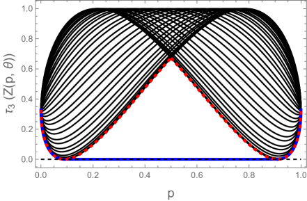
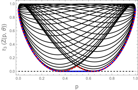
The is plotted in Fig. 2 when (a) and (b) with choosing from to as an interval . Both figures show that is minimized by
| (14) |
This curve is plotted in Fig. 2 as thick dashed red lines. Fig. 2 also show that at , where
| (15) |
One can show that is negative in some region depending on and between and . Therefore, , the convex hull of , can be written in a form
| (18) |
This is plotted in Fig. 2 as thick blue line.
IV Brief Review of HHL algorithm
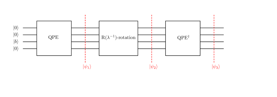
The HHL algorithmhhl consists of three steps, which are QPEQPE1 ; QPE2 ; QPE3 , -rotation, and inverse QPE. The schematic quantum circuit of the HHL algorithm is plotted in Fig. 3. These three steps were experimentally and explicitly realized in Ref. exp-hhl-1 444 In Fig. 1 of Ref. exp-hhl-1 the rotations and should be interchanged. by selecting a linear equation , where
| (23) |
where . If is not hermitian, one can change the linear equation by where is a hermitian matrix given by .
At the QPE stage we perform the QPE-algorithm by applying the unitary operator to . As shown in the appendix A, after the QPE stage the quantum state becomes
| (24) |
if one chooses . In Eq. (24) and are the eigenvalue and corresponding eigenvector of and is defined by . The last qubit is an ancilla, which will be used at the next stage. For the case of Eq. (23) we should choose and
| (25) | |||
Thus, if the QPE stage is perfectly implemented in quantum computer, the quantum state reduces to
| (26) |
In -rotation stage we implement the controlled rotations to the ancilla qubit, whose angles are proportional to . Using , the quantum state becomes approximately
| (27) |
after this stage, where is some appropriate nonzero constant. For the case of Eq. (23) is chosen as . If, therefore, this stage is perfectly implemented, after this stage becomes approximately
| (28) |
V tripartite entanglement in HHL algorithm
In this section we discuss how much the HHL algorithm utilizes the entanglement efficiently as we discussed previously in the Grover’s algorithm. In this reason we will compute the entanglement at each stage of the HHL algorithm. For simplicity, we will consider only the case of Eq. (23). Thus, the three-tangleckw and -tangleou07-1 will be computed explicitly after taking a partial trace over the ancilla qubit in Eqs. (26), (28), and (30).
Since the ancilla qubit is decoupled in of Eq. (26), the first three-qubit state after the QPE stage is simply
| (36) |
From Eq. (28) one can compute . It turns out that is rank- mixed state and its spectral decomposition is
| (37) |
where
| (38) |
In Eq. (37) and are the same with Eq. (8) if
| (39) |
where
| (40) | |||
Similarly, can be computed by making use of Eq. (30), whose spectral decomposition is
| (41) |
where
| (42) |
with
| (43) | |||
One can show explicitly. In Eq. (41) and are
| (44) |
where
| (45) |
with
| (46) |
V.1 Three-tangle
Using Ref. ckw it is easy to compute the three-tangle of :
| (47) |
From Eq. (15) for is
| (48) |
where and . Thus, making use of Eq. (18) one can compute the three-tangle of , whose explicit expression is
| (51) |
where with
| (52) |
Of course, , , and are given in Eqs. (38) and (40). Since and are fully separable states, the three-tangle of is
| (53) |
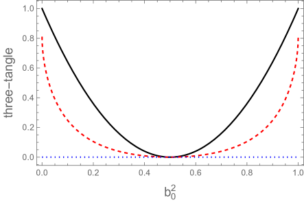
The three-tangles for , , and are plotted in Fig. 4(a) as a function of . The black solid, red dashed, and blue dotted lines correspond to , , and . From this figure we understand that the QPE stage generates the three-tangle represented by the black solid line. This three-tangle reduces to red dashed line in the -rotation stage. Finally, the matrix inversion task is accomplished in the stage at the price of complete annihilation of the three-tangle.
V.2 -tangle
The -tangle is a global negativityvidal01-1 -based tripartite entanglement measureou07-1 . While three-tangle cannot detect the tripartite entanglement of the W-state class, -tangle can detect it. For a three-qubit state the global negativities are given by
| (54) |
where , and the superscripts , and represent the partial transposes of with respect to the qubits , and respectively. Using the separability criterion based on partial transpose peres96 ; horod96 ; horod97 , it is easy to show that the global negativities vanish for separable states. It is worthwhile noting that the computation of the global negativities is relatively simple compared to the concurrence or three-tangle for mixed states since it does not need the convex-roof extension defined in Eq. (10). In addition, the negativities also satisfy the monogamy inequality
| (55) |
like concurrence. Then, the -tangle is defined as
| (56) |
where
| (57) |
It is easy to show that the -tangles for and become
| (58) |
where
| (59) |
Thus, the -tangle detects W-like(as well as GHZ-like) entanglement.
It is straightforward to compute the -tangle of , , and . The final result is
| (60) |
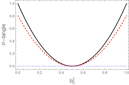
This is plotted in Fig. 4(b) as a function of . The black solid, red dashed, and blue dotted lines correspond to , , and . The behavior of the -tangle is similar to that of the three-tangle. The only difference is that is generally smaller than . This means that the decrease of -tangle in the -rotation stage is smaller compared to the three-tangle.
VI Conclusion
In this paper we examine a question ‘how much the HHL algorithm exploits the quantum entanglement efficiently?’. In this reason we computed the tripartite entanglement explicitly at the every steps of the HHL algorithm by choosing the explicit example (23).
As Fig. 4 shows, the three-tangle and -tangle exhibit similar behavior. At the QPE stage the tripartite entanglement is generated. The amount of it is dependent on . If or , maximal tripartite entanglement is generated at this stage. For other case partial entanglement is generated. At the -rotation stage some entanglement is used. Thus, the net tripartite entanglement is reduced. At the final stage the matrix inversion task is completed at the price of vanishing all entanglement.
The HHL algorithm is known as an optimalhhl in the matrix inversion task. It is also known that entanglement is a physical resource in quantum information processing. Then, the following question arises: why maximal creation of entanglement and complete annihilation of it do not occur? As discussed in Sec. II similar phenomenon happens in the Grover’s algorithm for large even though it is known to be optimalzalka99 in the quantum searching task. This means that from an aspect of entanglement, both algorithms do not use entanglement efficiently to some extent. We think there are additional quantities as well as entanglement, which may play important role in the quantum algorithm. Similar situation happens in the quantum illuminationlloyd08 ; tan08 ; eylee-22-1 . In this case the quantum discord is known to be importantdiscord1 ; discord2 .
Even though we have not presented explicitly in the paper, one can show that all bipartite entanglement of , , and are zero. This means that and are in the GHZ-classdur00-1 . We do not exactly understand why the W-type entanglement does not arise. All the questions will be discussed in the future.
References
- (1) M. A. Nielsen and I. L. Chuang, Quantum Computation and Quantum Information (Cambridge University Press, Cambridge, England, 2000).
- (2) E. Schrödinger, Die gegenwärtige Situation in der Quantenmechanik, Naturwissenschaften, 23 (1935) 807.
- (3) R. Horodecki, P. Horodecki, M. Horodecki, and K. Horodecki, Quantum Entanglement, Rev. Mod. Phys. 81 (2009) 865 [quant-ph/0702225] and references therein.
- (4) C. H. Bennett, G. Brassard, C. Crepeau, R. Jozsa, A. Peres and W. K. Wootters, Teleporting an Unknown Quantum State via Dual Classical and Einstein-Podolsky-Rosen Channles, Phys.Rev. Lett. 70 (1993) 1895.
- (5) Y. H. Luo et al., Quantum Teleportation in High Dimensions, Phys. Rev. Lett. 123 (2019) 070505 [arXiv:1906.09697 (quant-ph)].
- (6) C. H. Bennett and S. J. Wiesner, Communication via one- and two-particle operators on Einstein-Podolsky-Rosen states, Phys. Rev. Lett. 69 (1992) 2881.
- (7) V. Scarani, S. Lblisdir, N. Gisin and A. Acin, Quantum cloning, Rev. Mod. Phys. 77 (2005) 1225 [quant-ph/0511088] and references therein.
- (8) A. K. Ekert , Quantum Cryptography Based on Bell’s Theorem, Phys. Rev. Lett. 67 (1991) 661.
- (9) C. Kollmitzer and M. Pivk, Applied Quantum Cryptography (Springer, Heidelberg, Germany, 2010).
- (10) K. Wang, X. Wang, X. Zhan, Z. Bian, J. Li, B. C. Sanders, and P. Xue, Entanglement-enhanced quantum metrology in a noisy environment, Phys. Rev. A97 (2018) 042112 [arXiv:1707.08790 (quant-ph)].
- (11) T. D. Ladd, F. Jelezko, R. Laflamme, Y. Nakamura, C. Monroe, and J. L. O’Brien, Quantum Computers, Nature, 464 (2010) 45 [arXiv:1009.2267 (quant-ph)].
- (12) G. Vidal, Efficient classical simulation of slightly entangled quantum computations, Phys. Rev. Lett. 91 (2003) 147902 [quant-ph/0301063].
- (13) F. Arute et al.,Quantum supremacy using a programmable superconducting processor, Nature 574 (2019) 505. Its supplementary information is given in arXiv:1910.11333.
- (14) P. W. Shor, Algorithms for Quantum Computation: Discrete Logarithms and Factoring, Proc. 35th Annual Symposium on Foundations of Computer Science (1994) 124.
- (15) L. K. Grover, A fast quantum mechanical algorithm for database search, Proc. 28th Annual ACM Symposium on the Theory of Computing (1996) 212 [quant-ph/9605043].
- (16) A. W. Harrow, A. Hassidim, and S. Lloyd, Quantum algorithm for solving linear systems of equations, Phys. Rev. Lett. 15 (2009) 150502 [arXiv:0811.3171 (quant-ph)].
- (17) D. W. Berry, G. Ahokas, R. Cleve, and B. C. Sanders, Efficient quantum algorithms for simulating sparse Hamiltonians, Comm. Math. Phys. 270 (2007) 359 [arXiv:quant-ph/0508139 (quant-ph)].
- (18) L. Wossnig, Z. Zhao, and A. Prakash, A quantum linear system algorithm for dense matrices, Phys. Rev. Lett. 120 (2018) 050502 [arXiv:1704.06174 (quant-ph)].
- (19) Y. Lee, J. Joo, and S. Lee, Hybrid quantum linear equation algorithm and its experimental test on IBM Quantum Experience, Scientific Reports 9 (2019) 4778 [arXiv:1807.10651 (quant-ph)].
- (20) J. Pan, Y. Cao, X. Yao, Z. Li, C. Ju, X. Peng, S. Kais, and J. Du, Experimental realization of quantum algorithm for solving linear systems of equations, Phys. Rev. A 89 (2014) 022313 [arXiv:1302.1946 (quant-ph)].
- (21) V. Coffman, J. Kundu and W. K. Wootters, Distributed entanglement, Phys. Rev. A61 (2000) 052306 [quant-ph/9907047].
- (22) L. K. Grover, Quantum Mechanics helps in searching for a needle in a haystack, Phys. Rev. Lett. 79 (1997) 325 [quant-ph/9706033].
- (23) C H. Bennett, E. Bernstein, G. Brassard, and U. Vazirani, Strengths and Weaknesses of Quantum Computing, SIAM Journal on Computing, 26 (1997) 1510 [quant-ph/9701001].
- (24) M. Boyer, G. Brassard, P. Hoeyer, and A. Tapp, Tight bounds on quantum searching, Fortschritte der Physik, 46 (1998) 493 [quant-ph/9605034].
- (25) L. K. Grover, How fast can a quantum computer search?, quant-ph/9809029.
- (26) S. Hill and W. K. Wootters, Entanglement of a Pair of Quantum Bits, Phys. Rev. Lett. 78 (1997) 5022 [quant-ph/9703041].
- (27) W. K. Wootters, Entanglement of Formation of an Arbitrary State of Two Qubits, Phys. Rev. Lett. 80 (1998) 2245 [quant-ph/9709029].
- (28) C. Zalka, Grover’s quantum searching algorithm is optimal, Phys.Rev. A 60 (1999) 2746 [quant-ph/9711070].
- (29) W. Dür, G. Vidal, and J. I. Cirac, Three qubits can be entangled in two inequivalent ways, Phys. Rev. A62 (2000) 062314 [quant-ph/0005115].
- (30) C. H. Bennett, D. P. DiVincenzo, J. A. Smokin and W. K. Wootters, Mixed-state entanglement and quantum error correction, Phys. Rev. A54 (1996) 3824 [quant-ph/9604024].
- (31) A. Uhlmann, Fidelity and concurrence of conjugate states, Phys. Rev. A 62 (2000) 032307 [quant-ph/9909060].
- (32) R. Lohmayer, A. Osterloh, J. Siewert and A. Uhlmann, Entangled Three-Qubit States without Concurrence and Three-Tangle, Phys. Rev. Lett. 97 (2006) 260502 [quant-ph/0606071].
- (33) A. Osterloh, J. Siewert, and A. Uhlmann, Tangles of superpositions and the convex-roof extension, Phys. Rev. A 77 (2008) 032310 [arXiv:0710.5909 (quant-ph)].
- (34) E. Jung, M. R. Hwang, D. K. Park and J. W. Son, Three-tangle for Rank- Mixed States: Mixture of Greenberger-Horne-Zeilinger, W and flipped W states, Phys. Rev. A79 (2009) 024306, arXiv:0810.5403 (quant-ph).
- (35) E. Jung, M. R. Hwang, D. K. Park, and S. Tamaryan, Three-Party Entanglement in Tripartite Teleportation Scheme through Noisy Channels, Quant. Inf. Comp. 40 (2010) 0377 [arXiv:0904.2807 (quant-ph)].
- (36) R. Cleve, A. Ekert, C. Macchiavello, and M. Mosca, Quantum Algorithms Revisited, quant-ph/9708016.
- (37) A. Luis and J. Per̆ina, Optimum phase-shift estimation and the quantum description of the phase difference, Phys. Rev. A 54 (1996) 4564.
- (38) see also https://qiskit.org/textbook/ch-algorithms/quantum-phase-estimation.html.
- (39) Y. U. Ou and H. Fan, Monogamy Inequality in terms of Negativity for Three-Qubit States, Phys. Rev. A75 (2007) 062308 [quant-ph/0702127].
- (40) G. Vidal and R. F. Werner, Computable measure of entanglement, Phys. Rev. A65 (2002) 032314 [quant-ph/0102117].
- (41) A. Peres, Separability Criterion for Density Matrices, Phys. Rev. Lett. 77 (1996) 1413 [quant-ph/9604005].
- (42) M. Horodecki, P. Horodecki and R. Horodecki, Separability of mixed states: necessary and sufficient conditions, Phys. Lett. A 223 (1996) 1 [quant-ph/9605038].
- (43) P. Horodecki, Separability criterion and inseparable mixed states with partial transposition, Phys. Lett. A 232 (1997) 333 [quant-ph/9703004].
- (44) S. Lloyd, Enhanced Sensitivity of Photodetection via Quantum Illumination, Science, 321, 1463 (2008).
- (45) S.-H. Tan, B. I. Erkmen, V. Giovannetti, S. Guha, S. Lloyd, L. Maccone, S. Pirandola, and J. H. Shapiro, Quantum Illumination with Gaussian States, Phys. Rev. Lett. 101, 253601 (2008) [arXiv:0810.0534 (quant-ph)].
- (46) E. Jung and D. K. Park, Quantum Illumination with three-mode Gaussian State, Quant. Inf. Proc. 21 (2022) 71 [arXiv:2107.05203 (quant-ph)].
- (47) C. Weedbrook, S. Pirandola, J. Thompson, V. Vedral, and M. Gu, How discord underlies the noise resilience of quantum illumination, New J. Phys. 18 (2016) 043027.
- (48) M. Bradshaw, S. M. Assad, J. Y. Haw, S. H. Tan, P. K. Lam, M. Gu, Overarching framework between Gaussian quantum discord and Gaussian quantum illumination, Phys. Rev. A 95 (2017) 022333 [arXiv:1611.10020 (quant-ph)].
-
(49)
see also https://qiskit.org/textbook/ch-algorithms/quantum-fourier-transform.html.
Appendix A: Quantum Phase Estimation (QPE)
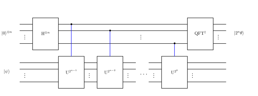
In this appendix QPE will be discussed in detail and Eq. (24) will be derived explicitly. The quantum circuit of QPEQPE3 is plotted in Fig. 5. In Fig. 5 QFT stands for quantum Fourier transformtext ; shor94 ; QFT1 , which is defined by the unitary operator obeying
| (A.1) |
where is arbitrary -qubit state and . As Fig. 5 shows, QPE consists of two registers. First register starts with , which we will call ‘c-register’. Second register starts with some quantum state , which we will call ‘t-register’. In the figure is a certain unitary operator.
If is an eigenvector of in a form
| (A.2) |
the quantum circuit in Fig. 5 generates in the c-register and t-register respectively at the final stage. If the whole process of QPE is represented by an unitary operator , this fact implies
| (A.3) |
Thus, measuring the c-register at the final step, one can estimate the phase . For example, if the outcome is , one can conjecture 555If is not a form of , the quantum circuit produces an inequality , where decreases with increasing .
Now, let us consider the case that is not an eigenvector of . Let the eigenvectors of be obeying
| (A.4) |
Since a set is a complete, can be expressed as a linear combination of in a form
| (A.5) |
Using a fact that is a linear operator, it is straightforward to show
| (A.6) |
in this case.
Since and in the HHL algorithm and they obey
| (A.7) |
the final state after QPE becomes
| (A.8) |
Thus, if is chosen as , one can derive Eq. (24).