Delving into the Estimation Shift of Batch Normalization in a Network

Abstract

Batch normalization (BN) is a milestone technique in deep learning. It normalizes the activation using mini-batch statistics during training but the estimated population statistics during inference. This paper focuses on investigating the estimation of population statistics. We define the estimation shift magnitude of BN to quantitatively measure the difference between its estimated population statistics and expected ones. Our primary observation is that the estimation shift can be accumulated due to the stack of BN in a network, which has detriment effects for the test performance. We further find a batch-free normalization (BFN) can block such an accumulation of estimation shift. These observations motivate our design of XBNBlock that replace one BN with BFN in the bottleneck block of residual-style networks. Experiments on the ImageNet and COCO benchmarks show that XBNBlock consistently improves the performance of different architectures, including ResNet and ResNeXt, by a significant margin and seems to be more robust to distribution shift.

1 Introduction

Input normalization is extensively used in training neural networks for decades [20] and shows good theoretical properties in optimization for linear models [21, 50]. It uses population statistics for normalization that can be calculated directly from the available training data. A natural idea is to extend normalization for the activation in a network. However, normalizing activation is more challenging since the distribution of internal activation varies, which leads to the estimation of population statistics for normalization inaccurate [30, 7]. A network with activation normalized by the population statistics shows the training instability [12].

Batch normalization (BN) [17] addresses itself to normalize the activation using mini-batch statistics during training, but the estimated population statistics during inference/test. BN ensures the normalized mini-batch output standardized over each iteration, enabling stable training, efficient optimization  [17, 1, 39, 13] and potential generalization [13, 3, 51]. It has been extensively used in varieties of architectures [9, 48, 57, 47, 11, 53], and successfully proliferated throughout various areas [37, 25, 12].

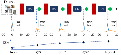
(a)

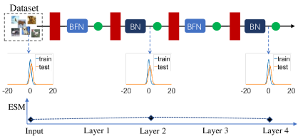
(b)

Figure 1: Illustration of the main observations. The red rectangle and green round represent a linear and non-linear transformation, respectively. Given the training and test data with distribution shift, we show the distributions of normalized output after each BN layer during training and test, and calculate the magnitude of difference between the estimated population statistics and expected ones (refer to as ESM, and see Section 4.2 for details).

Despite the common success of BN, it still suffers from problems when applied in certain scenarios [12, 4]. One notorious limitation of BN is its small-batch-size problem — BN’s error increases rapidly as the batch size becomes smaller [51, 44]. Besides, a network with a naive BN gets significantly degenerated performance, if there exists covariate shift between the training and test data [23, 40, 31, 2]. While these problems raise across different scenarios and contexts, the estimated population statistics of BN used for inference seems to be the link between them: 1) the small-batch-size problem of BN can be relieved if its estimated populations statistics are corrected during test [44, 46]; 2) and a model is more robust for unseen domain data (corrupted images) if the estimated population statistics of BN are adapted based on the available test data [23, 40, 2].

This paper investigates the estimation of population statistics in a systematic way. We introduce expected population statistics of BN, considering the ill-defined population statistics of the activation with a varying distribution during training (see Section 4.2 for details). We refer to as estimation shift of BN if its estimated population statistics do not equal to its expected ones, and design experiments to quantitatively investigate how the estimation shift affects a batch normalized network.

Our primary observation is that the estimation shift of BN can be accumulated in a network (Figure 1 (a)). This observation provides clues to explain why a network with BN has significantly degenerated performance under small-batch-size training, and why the population statistics of BN need to be adapted if there exists distribution shift for input data during test. We further find that a batch-free normalization (BFN)—normalizing each sample independently without across batch dimension—can block the accumulation of the estimation shift of BN. This relieves the performance degeneration of a network if a distribution shift occurs.

These observations motivate our design of XBNBlock that replaces one BN with BFN in the bottleneck of residual-style networks [9, 53]. We apply the proposed XBNBlock to ResNet [9] and ResNeXt [53] architectures and conduct experiments on the ImageNet [37] and COCO [25] benchmarks. XBNBlock consistently improves the performance for both architectures, with absolute gains of $0.6\%\sim 1.1\%$ in top-1 accuracy for ImageNet, $0.86\%\sim 1.62\%$ in bounding box AP for COCO using Faster R-CNN [36], and $0.56\%\sim 2.06\%$ ( $0.22\%\sim 1.18\%$) in bounding box AP (mask AP) for COCO using Mask R-CNN [8]. Besides, XBNBlock seems to be more robust to the distribution shift.

2 Related Work

Estimating and exploiting population statistics.

Batch normalization (BN) suffers from small-batch-size problem, since the estimation of population statistics could be inaccurate. To address this issue, a variety of batch-free normalization (BFN) are proposed [1, 51, 22], e.g., layer normalization (LN) [1] and group normalization (GN) [1]. These works perform the same normalization operation for each sample during training and inference. Another way to reduce the discrepancy between training and inference is to combine the estimated population statistics with mini-batch statistics for normalization during training [16, 6, 54, 43, 56, 55]. These work may outperform BN trained with a small batch size, where estimation is the main issue[17, 18, 27], but they usually have inferior performance when the batch size is moderate.

Some works focus on estimating corrected normalization statistics during inference only, either for domain adaptation [23], corruption robustness [40, 31, 2], or small-batch-size training  [44, 46]. These strategies do not affect the training scheme of the model. Li et al. [23] propose adaptive batch normalization (AdaBN) for domain adaptation, where the estimation of BN statistics for the available target domain is modulated during test. This idea is further exploited to improve robustness under covariate shift of the input data with corruptions [40, 2]. Another line of works correct the normalization statistics for small-batch-size training by optimizing  [44, 46] the sample weight during inference, seeking for that the normalized output by population statistics are similar to those observed using mini-batch statistics during training. Besides, there are works considering the prediction-time batch settings [45, 31] for deep generative model [45] and preventing covariate shift of the test data [31], where the mini-batch statistics from the test data are used for inference.

Compared to the works shown in above, our work focuses on investigating the estimation shift of BN in a network. Our observation, that the estimation shift of BN can be accumulated in a network, provides clues to explain why a network with stacked BNs has significantly degenerated performance under small-batch-size training, and why the population statistics of BN in each layer needs to be adapted if there exists covariate shift for input data during test. Besides, we design XBNBlock with BN and BFN mixed to block the accumulation of estimation shift of BNs.

Combining BN with other normalization methods.

Researches have also be conducted to build a normalization module in a layer by combining different normalization strategies. Luo et al. propose switchable normalization (SN) [27], which switches among the different normalization methods by learning their importance weights, computed by a softmax function. This idea is further extended by introducing the sparsity constraints [42], whitening operation [34], and dynamic calculation of the importance weights [59]. Other methods address the combination of normalization methods in specific scenarios, including image style transfer [32], image-to-image translation [19], domain generalization [41] and meta-learning scenarios [5]. Different from these methods which aim to build a normalization module in a layer, our proposed XBNBlock is a building block with BN and BFN mixed in different layers. Furthermore, our observation, that a BFN can block the accumulation of estimation shift of BNs in a network, provides a new view to explain the successes of above methods combining BN with other normalization methods.

Our work is closely related to IBN-Net [33], which carefully integrates instance normalization (IN) [49] and BN as building blocks, and can be wrapped into several deep networks to improve their performances. Note that IBN-Net carefully designs the position of an IN and its channel number, while the design of our XBNBlock is simplified. Moreover, IBN-Net is motivated by that IN can learn style-invariant features [49] thus benefiting generalization, while our XBNBlock is motivated by that a BFN can relieve the estimation shift of BN, thus avoiding its degenerated test performance if inaccurate estimation exists. Here, we highlight our observation that a BFN (e.g., IN) can block the accumulation of estimation shift of BNs also provide a reasonable explanation to the success of IBN-Net in its test performance, especially in the scenarios with distribution shift [33].

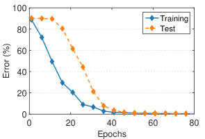
(a)

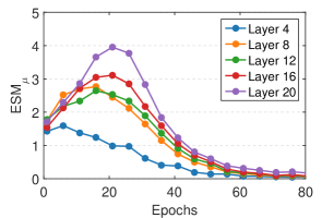
(b)

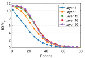
(c)

Figure 2: Experiments with the training set $\mathbf{S}$ equaling to the test set $\mathbf{S^{\prime}}$. We train a 20-layer MLP with 128 neurons in each layer for MNIST classification. $\mathbf{S}$ and $\mathbf{S^{\prime}}$ are the original test set of MNIST with 10,000 samples. We use full-batch gradient descent to train 80 epochs (iterations) with a learning rate of 0.1. The estimated population statistics of BN are calculated by the commonly used running average (Eqn. 2) with update factor $\alpha=0.9$. We also try other configurations (e.g., varying the learning rate, update factor $\alpha$ and depth of the network), and further conduct experiments on convolutional neural networks (CNNs). We obtain similar results (see Appendix  A for details).

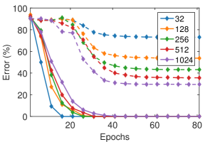
(a)

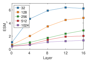
(b)

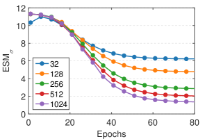
(c)

Figure 3: Experiments using the training set $\mathbf{S}$ sampled from the test set $\mathbf{S^{\prime}}$. We follow the same experimental setup in Figure 2 except that we use the training set with varying size $|\mathbf{S}|=\{32,128,256,512,1024\}$. We use $\|\sqrt{\sigma^{2}_{train}}-\sqrt{\sigma^{2}_{test}}\|_{2}$ to evaluate the distribution shift of the input (referred to as $ESM_{\sigma}$ w.r.t.  layer 0), where $\sigma^{2}_{train}$ ($\sigma^{2}_{test}$) is the variance of the training (test) set.

3 Preliminary

Batch normalization.

Let $\mathbf{x}\in\mathbb{R}^{d}$ be the $d$-dimensional input to a given layer of multi-layer perceptron (MLP). During training, batch normalization normalizes each neuron/channel within $m$ mini-batch data by

$$\hat{\mathbf{x}}_{j}=BN_{train}(\mathbf{x}_{j})=\frac{\mathbf{x}_{j}-\mu_{j}}{\sqrt{\sigma^{2}_{j}+\epsilon}},~{}~{}j=1,2,...,d,$$ (1)

where $\mu_{j}=\frac{1}{m}\sum_{i=1}^{m}\mathbf{x}_{j}^{(i)}$ and $\sigma^{2}_{j}=\frac{1}{m}\sum_{i=1}^{m}(\mathbf{x}_{j}^{(i)}-\mu_{j})^{2}$ are the mini-batch mean and variance for each neuron, respectively, and $\epsilon$ is a small number to prevent numerical instability. During inference/test, the population mean $\tilde{\mu}$ and variance $\tilde{\sigma}^{2}$ of the layer input are required for BN to make a deterministic prediction [17] as:

$$\hat{\mathbf{x}}_{j}=BN_{inf}(\mathbf{x}_{j})=\frac{\mathbf{x}_{j}-\tilde{\mu}_{j}}{\sqrt{\tilde{\sigma}^{2}}},~{}~{}j=1,2,...,d.$$ (2)

Even though the population statistics $\{\tilde{\mu},\tilde{\sigma}^{2}\}$ of the layer input are ill-defined (illustrated in Section 4.1), their estimation $\{\hat{\mu},\hat{\sigma}^{2}\}$ are usually used in Eqn. 2 by calculating the running average of mini-batch statistics over different training iterations $t$ with an update factor $\alpha$ as follows:

$$\begin{cases}\quad\hat{\mu}^{t}=(1-\alpha)\hat{\mu}^{t-1}+\alpha\mu^{t-1},\\ \quad(\hat{\sigma}^{t})^{2}=(1-\alpha)(\hat{\sigma}^{t-1})^{2}+\alpha(\sigma^{t-1})^{2}.\end{cases}$$ (3)

The discrepancy of BN during training and inference limits its usage in recurrent neural network [1], or harms the performance for small-batch-size training [51], since the estimation of population statics can be inaccurate.

Batch-free normalization.

There exists batch-free normalization for avoiding normalization along the batch dimension, and thus avoiding the estimation of population statistics. These methods use consistent operations during training and inference. One representative method is layer normalization (LN) [1] that standardizes the layer input within the neurons for each training sample, as:

$$\hat{\mathbf{x}}_{j}=LN(\mathbf{x}_{j})=\frac{\mathbf{x}_{j}-\mu}{\sqrt{\sigma^{2}+\epsilon}},~{}~{}j=1,2,...,d,$$ (4)

where $\mu=\frac{1}{d}\sum_{i=1}^{d}\mathbf{x}_{j}$ and $\sigma^{2}=\frac{1}{d}\sum_{i=1}^{d}(\mathbf{x}_{j}-\mu)^{2}$ are the mean and variance for each sample, respectively. LN is further generalized by group normalization (GN) [51] that divides the neurons into groups and performs the standardization within the neurons of each group independently. By changing the group number, GN is more flexible than LN, enabling it to achieve good performance on visual tasks limited to small-batch-size training (e.g., object detection and segmentation [51]). While these BFN methods can work well on certain scenarios, they cannot match the performance of BN in most situations and are not commonly used in CNN architectures.

4 Estimation Shift of Batch Normalization

We begin with illustrating the ill-defined population statics of BN, and then design comprehensive experiments for investigating the estimation shift of BN.

4.1 Expected Population Statistics of BN

Let $\mathbf{S}$ be the training set and $\{S^{t}\}_{t=1}^{T}$ the mini-batch data sampled from $\mathbf{S}$ during training. Considering a neural network with a BN $F_{\psi,\theta}(S)=F^{post}_{\psi}(BN(F^{pre}_{\theta}(S)))$, we denote $X=F^{pre}_{\theta}(S)$ and $\widehat{X}=BN(X)$. The population statistics of the certain training set $\mathbf{S}$ are well-defined and they can be well estimated straightforwardly using the mini-batch statistics of $\{S^{t}\}_{t=1}^{T}$. However, the population statistics of the activation $\mathbf{X}=F^{pre}_{\theta}(\mathbf{S})$ are ill-defined, because $\mathbf{X}$ is varying during training due to the update of parameter $\theta$ in each iteration. Indeed, the mini-batch samples of $\mathbf{X}$ are $X^{t}=F^{pre}_{\theta^{t}}(S^{t}),$ for$~{}t=1,...,T$, which depends not only on the mini-batch input $S^{t}$, but also on the model sequences $\{F^{pre}_{\theta^{t}}(\cdot)\}_{t=1}^{T}$. Therefore, the population statistics of $\mathbf{X}$ should be a function of the training set $\mathbf{S}$ and the varying model sequences $\{F^{pre}_{\theta^{t}}(\cdot)\}_{t=1}^{T}$ during training. Even though it is difficult to explicitly define the population statistics of $\mathbf{X}$ from the statistical view, we note that the mini-batch input $\widehat{X}^{t}$ of sub-network $F^{post}_{\psi}(\cdot)$ is always a standardized distribution for each iteration. Therefore, the ideal population statistics of $\mathbf{X}$ should ensure the normalized output standardized over the test set. We implicitly define the expected population statistics of BN as follows.

Definition 1

Let $F_{\tilde{\psi},\tilde{\theta}}(\cdot)$ be the trained model on training set $\mathbf{S}$. Given the test set $\mathbf{S^{\prime}}$, we refer to $\{\tilde{\mu},\tilde{\sigma}^{2}\}$ are the expected population statistics of BN, where $\tilde{\mu}$ ($\tilde{\sigma}^{2}$) is the mean (variance) of BN’s input $\mathbf{X}=F^{pre}_{\tilde{\theta}}(\mathbf{S^{\prime}})$.

Note that the expected population statistics of BN are defined on the trained model $F_{\tilde{\psi},\tilde{\theta}}(\cdot)$ conditioned on the input from the test set $\mathbf{S^{\prime}}$ rather than the training set $\mathbf{S}$, because the population statistics of $\mathbf{X}=F^{pre}_{\tilde{\theta}}(\mathbf{S})$ consider only the last trained model $F^{pre}_{\tilde{\theta}}(\cdot)$ rather than the model sequences $\{F^{pre}_{\theta^{t}}(\cdot)\}_{t=1}^{T}$. Indeed, the population statistics of $\mathbf{X}=F^{pre}_{\tilde{\theta}}(\mathbf{S})$ can be readily calculated once the model is trained, as introduced in  [17, 27, 52]. However, they usually have worse generalization performance than the one used by running average shown in Eqn. 3.

4.2 An Investigation into the Estimation Shift

Given the expected population statistics of the BN defined, we refer to as estimation shift of BN if its estimated population statistics do not equal to its expected ones. It is important to investigate how the estimation shift of BN affects the performance of batch normalized network. We thus seek to quantitatively measure the magnitude of the difference between estimated statistics and its expected ones.

Definition 2

Let $\tilde{\mu}$ ($\tilde{\sigma}^{2}$) is the expected population mean (variance) of BN and $\hat{\mu}$ ($\hat{\sigma}^{2}$) is the estimated one. We define the estimation shift magnitude (ESM) as the $L^{2}$-norm of their difference. E.g., $ESM_{\mu}=\|\hat{\mu}-\tilde{\mu}\|_{2}$ and $ESM_{\sigma}=\|\sqrt{\hat{\sigma}^{2}}-\sqrt{\tilde{\sigma}^{2}}\|_{2}$.

In the following sections, we design experiments to investigate how the estimation shift  of BN affects the performance of batch normalized network and how it can be rectified.

4.2.1 Accumulation of Estimation Shift in a Network

We consider two experimental setups: 1) in setup one, we use the training set $\mathbf{S}$ equaling to the test set $\mathbf{S^{\prime}}$ for investigating estimation shift of BN under the scenario without distribution shift of the input data; 2) in setup two, the training set $\mathbf{S}$ is sampled from the test set $\mathbf{S^{\prime}}$. We vary the size of $\mathbf{S}$ to modulate the distribution shift between training and test set.

Setup one.

The details of experimental setup and the results are shown in Figure 2. We observe that there are significant gaps between the training and test errors in the first 30 epochs. Note that the training and test errors in this setup should be the same over iterations if BN adopts the same operation during training and inference. In Figure 2 (b) and (c), $ESM_{\mu}$ and $ESM_{\sigma}$ of BN in certain layers are significantly larger than zero in the first 30 epochs and then gradually converge to zero. This phenomenon clearly shows that the error gaps between training and test are mainly caused by the inaccurate estimation of the population statistics of BN.

One important observation is that the $ESM_{\mu}$ and $ESM_{\sigma}$ of BN in deeper layers have potentially higher values during the first 30 epochs. This observation implies that the estimation of BN in lower layers will affect the one in upper layer. The estimation shift of BN in upper layer will be amplified if the BN in lower layer suffers from estimation shift which causes a distribution shift of the input into upper layer between training and test. Therefore, the inaccurate estimation of population statistics can be potentially accumulated/compounded due to the stack of BN layers.

Setup two.

In this setup, the training set $\mathbf{S}$ is sampled from the test set $\mathbf{S^{\prime}}$ and we vary the size of training set $|\mathbf{S}|$ to modulate the distribution shift between the training and test set. We expect to see how the varying distribution shift affects the estimation of BN’s population statistics in a network. The details of experimental setup and results are shown in Figure 3. We find that the distribution shift can be potentially larger when decreasing the size of sampled training set from Figure 3 (b). Furthermore, the $ESM_{\sigma}$ of all the BN layers are significantly larger than zero, and a BN layer in a model trained with fewer samples has higher $ESM_{\sigma}$. Besides, in Figure 3 (a), we observe that all the models can be trained with an zero training error, while the test error is significantly higher if a model is trained on the training set with fewer samples. These observations imply that the distribution shift of the input between the training and test set can cause the estimation shift of BN, which has a detriment effect on the test performance. E.g., we find that the model without BN obtains a test error of $57.73\%$ when using 32 training samples, compared to the model with BN having a test error of $73.02\%$.

One important observation is that $ESM_{\sigma}$ of BN in deeper layers have potentially higher value at the end of training. This observation shows remarkable evidences to support that the estimation shift of BN can be accumulated due to the stack of BN layers. Moreover, the estimation shift is graver if the model is trained with fewer training samples and stronger distribution shift of the input data.

Here, we highlight that it is important to define the expected population statistics of BN on $F_{\tilde{\theta}}(\mathbf{S^{\prime}})$ rather than $F_{\tilde{\theta}}(\mathbf{S})$. We note that the $ESM_{\sigma}$ of BN gradually converges to a stable value (Figure  3 (c)) in this experiment, which suggests that the estimation used by the running average (Eqn. 2) converges to the estimation on the trained model over the training set [17, 27] (i.e., $F_{\tilde{\theta}}(\mathbf{S})$). $ESM_{\sigma}$ will be zero if $ESM_{\sigma}$ is define on $F_{\tilde{\theta}}(\mathbf{S})$. This is not what we expect, because it provides no information to diagnose the degenerated test performance of a model trained on the training set with fewer samples that suffers larger distribution shift over the test set, as shown in this experiment.

In summary, according to the experiments above, we argue that estimation shift of BN can be potentially accumulated in a network with stacked BNs, which probably has a detriment effect on the test performance of the network, especially with the distribution shift occurred.

(a)

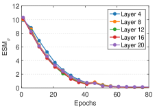
(b)

Figure 4: Experiments on a network with BN and GN mixed. We follow the same setup shown in Figure 2, except that we replace the BNs of the odd layers with GNs in the network (referred to as ‘GNBN’). Here, we use GN with a group number of 4. We also try different group numbers and obtain similar observations (see Appendix  A for details).

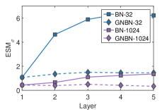
(a)

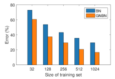
(b)

Figure 5: Experiments on a network with BN and GN mixed. We follow the same setup shown in Figure 3, except that we replace the BNs of odd layers with GNs in the network. Here, ‘-N’ indicates that the model is trained on the training set with N samples.

4.2.2 Blocking the Accumulation of Estimation Shift

We experimentally show that the accumulation of estimation shift of BN can be relieved if a BFN is inserted in a network. We replace the BNs of the odd layers with GNs, and refer to this network as ‘GNBN’. We follow the previous two experimental setups shown in Section 4.2.1 and show the results in Figure 4 and 5, respectively. We find that the error gaps between the training and test are significantly reduced in the first 30 epochs from Figure 4 (a). Importantly, we observe that $ESM_{\sigma}$ of BN among all layers are nearly the same during training from Figure 4 (b). This implies that the GN in the odd layer potentially blocks the accumulation of estimation shift of BNs in its two adjacent layers.

In Figure 5(a), we observe that $ESM_{\sigma}$ of BNs in the ‘GNBN’ is significant lower than the original network (‘BN’). Furthermore, there is no remarkable difference for $ESM_{\sigma}$ of BN among different layers at the end of training. These observations further corroborate that GN can block the accumulation of estimation shift of BNs in its two adjacent layers. We attribute this to the consistent operation of GN between training and inference (for each sample) which ensures that the input of later layers have nearly the same distribution. The blocked accumulation of estimation shift ensures a significantly improved performance for a network, as shown in the comparison of ‘GNBN’ to ‘BN’ in Figure 5(b).

According to the experiments above, we argue that a BFN (e.g., GN) can block the accumulation of estimation shift of BN in a network, which can relieve the performance degeneration of a network if distribution shifts exist.

5 Evaluation on Visual Recognition Tasks

In this section, we first design a kind of convolution block, and then validate its effectiveness on ImageNet classification [37], as well as COCO detection and segmentation [25].

5.1 Proposed XBNBlock

We design XBNBlock that replaces one BN with BFN in the bottleneck (Figure 6 (a)) which is widely used in the residual-style networks [9, 53]. Figure 6 (b) shows the proposed ‘XBNBlock-P2’ in which we replace the second BN layer with BFN. We also consider other positions and compare their performance in Section 5.2.1.

For the convolutional input $\mathbf{X}\in\mathbb{R}^{d\times m\times H\times W}$, where $H$ and $W$ are the height and width of the feature maps, BN and BFN used in CNNs both calculate the mean/variance over the $H$ and $W$ dimensions. This paper mainly uses GN as BFN (referred to as XBNBlock_GN), considering GN is more flexible to control the constraints on the distribution of normalized output by changing its group number [15]. We also experiments with IN which calculates the mean/variance only over the $H$ and $W$ dimensions for each channel of a sample, and provides stronger constraints on the normalized output. E.g., IN ensures the distribution of each channel standardized, while GN ensures the distribution of each group (multiple channels) standardized.

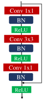
(a)

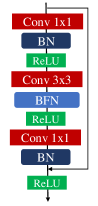
(b)

Figure 6: Bottleneck vs  our ‘XBNBlock-P2’ that replaces the second BN of a bottleneck with a BFN.

Methods	Accuracy (%)
Baseline (BN)	76.29
GN	75.73
XBNBlockGN-P1	77.08
XBNBlockGN-P2	77.40
XBNBlockGN-P3	76.76

Table 1: Results of different positions when applying a GN in XBNBlock. We evaluate the top-1 validation accuracy.

5.2 ImageNet Classification

We conduct experiments on the ImageNet dataset with 1,000 classes  [37]. We use the official 1.28M training images as a training set, and evaluate the top-1 accuracy on a single-crop of 224$\times$224 pixels in the validation set with 50k images. Our implementation is based on PyTorch [35]. We mainly apply our XBNBlock in the ResNet [9] and ResNeXt [53] models to validate its effectiveness. Please refer to Appendix B.1 for more results on other architectures.

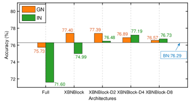
Figure 7: Top-1 validation accuracy of different positions when applying a XBNBlock in a network. ‘Full’ indicates a network with all the BNs replaced with GN/IN.

Figure 8: Top-1 validation accuracy with different noise magnitudes imposed on the estimated population statistics. The results are averaged over 5 random seeds. We refer to a bottleneck/XBNBlock as ‘disturbed block’ if its first BN uses $\{\hat{\mu}_{\delta},\hat{\sigma}^{2}_{\delta}\}$ for normalization during inference. Here the first six blocks of ResNet-50 are ‘disturbed block’. We also perform experiments using other blocks as ‘disturbed block’ and obtain similar observations (see Appendix B for details).

Method	ResNet-50	ResNet-101	ResNeXt-50	ResNeXt-101
Baseline (BN) [17]	76.29	77.65	77.06	79.17
GN [51]	75.73	77.18	75.67	78.02
IBN-Net* [33]	77.46	78.61	–	79.12
SN* [27]	76.90	77.99	–	–
XBNBlockGN (ours)	77.40	78.21	77.66	79.84
XBNBlockGN-D2 (ours)	77.39	78.63	77.63	79.72

Table 2: Top-1 accuracy ($\%$) on ResNets [9] and ResNeXts [53] for ImageNet. ‘*’ indicates the results are from the corresponding papers.

	LS	MixUp	COS	LS + MixUP + COS
Baseline (BN)	76.70	76.75	76.72	77.16
XBNBlockGN	77.41	77.70	77.60	78.22

Table 3: Top-1 accuracy ($\%$) on ResNet-50 using advanced training strategies. ‘LS’ indicates label smoothing and ‘COS’ indicates cosine learning rate decay.

5.2.1 Ablation Studies on ResNet-50

We adopt the widely used training protocol to compare the performance of ResNets/ResNeXt for ImageNet classification [9]: we apply stochastic gradient descent (SGD) using a mini-batch size of 256, momentum of 0.9 and weight decay of 0.0001. We train over 100 epochs. The initial learning rate is set to 0.1 and divided by 10 at 30, 60 and 90 epochs. Our baseline is the ResNet-50 trained with BN [17].

Positions of BFN in an XBNBlock.

We investigate the position where to apply BFN in an XBNBlock. We use GN (with group number $g$=64) as BFN. We consider three XBNBlock variants that replace the first, second and third BN in the bottleneck and refer to them as ‘XBNBlock-P1’, ‘XBNBlock-P2’ and ‘XBNBlock-P3’, respectively. We substitute these XBNBlocks for all the bottlenecks of ResNet-50 and report the results in Table 1. We can see that all the networks with XBNBlock outperform the baseline by a clear margin. Note that the network in which all the BNs are replaced with GNs has only $75.63\%$ validation accuracy, which is worse than the baseline. This result implies that the estimation shift of BN probably exists due to the accumulation of multiple stacked BNs, even for training under a moderate batch-size. GN can block the accumulation of estimation shift of BN and thus improve the performance of the network with BN. We observe that ‘XBNBlock-P2’ obtain the best performance, and we refer to ‘XBNBlock-P2’ (Figure 6) as our XBNBlock by default in the following experiments.

Positions of XBNBlock in a network.

We also investigate the positions where to apply XBNBlock in a network. There are 16 bottlenecks in ResNet-50, and we consider three variants to alternatively substitute XBNBlocks for the bottlenecks: (1) XBNBlock-D2: the $\{2n,n=1,2,...,8\}$-th bottlenecks are replaced with XBNBlocks; (2) XBNBlock-D4: the $\{4n,n=1,2,3,4\}$-th bottlenecks are replaced with XBNBlocks; (3) XBNBlock-D8: the $\{8n,n=1,2\}$-th bottlenecks are replaced with XBNBlocks. We investigate GN and IN in the XBNBlock and refer to as ‘XBNBlock_GN’ and ‘XBNBlock_IN’. The results are shown in Figure 7. We observe that all the ‘XBNBlock_GN’ models have better validation accuracy than the baseline, and a network with fewer XBNBlock_GN has worse performance. We also find that ‘XBNBlock_IN-D4’ obtains a validation accuracy of $77.19\%$, better than the baseline ( $76.29\%$) while XBNBlock_IN has only $74.99\%$. We attribute this phenomenon to that IN provides stronger constraints on the normalized output, which can affect the representation ability of the model, e.g., XBNBlock_IN has only a training accuracy of $77.93\%$, significantly lower than the baseline with $80.29\%$ training accuracy. In the following section, we show that such constraints make a model more robust.

Robustness to distribution shift.

As discussed in Section 4.2.2, a BFN can block the accumulation of the estimation shift of BN, which suggests that a model with BFN could be more robust than the distribution shift. We design experiments to validate this arguments. We disturb the estimated mean and variance of BN as follows:

$$\begin{cases}\quad\hat{\mu}_{\delta}=(1+\delta_{\mu})\hat{\mu},~{}~{}~{}~{}\delta_{\mu}\sim uniform(-\Delta,\Delta)\\ \quad\hat{\sigma}^{2}_{\delta}=(1+\delta_{\sigma})\hat{\sigma}^{2},~{}~{}~{}~{}\delta_{\sigma}\sim uniform(-\Delta,\Delta),\end{cases}$$ (5)

where $\Delta$ represents noise magnitude. Figure 8 shows that the baseline (‘BN’) has significantly reduced validation accuracy as noise magnitude increases, while XBNBlock_GN/XBNBlock_IN is more stable for such a disturbance. This suggests that the consistent normalization operations during training and inference of a BFN can potentially reduce the distribution shift in a layer and improve the robustness of models. We also note that XBNBlock_IN is more robust than XBNBlock_GN, we attribute this to that IN indeed provides stronger constraints than GN on the normalized output, which gives a more stable distribution to prevent the distribution shift.

	ResNet-50				ResNext-101
	2fc head box		4conv1fc head box		2fc head box		4conv1fc head box
Method	APbbox	APmask	APbbox	APmask	APbbox	APmask	APbbox	APmask
$BN^{{\dagger}}$	37.40	34.01	37.51	33.68	42.13	37.78	42.24	37.53
GN	37.55	34.06	39.02	34.37	41.47	37.17	42.18	37.53
XBNBlockGN	38.19	34.57	39.57	34.86	42.69	38.00	43.43	38.68

Table 4: Detection and segmentation results ($\%$) on COCO using the Mask R-CNN framework implemented in [29]. Models based on ResNet-50 backbone are trained by 1x lr scheduling (90k iterations), with a batch size of 16 on eight GPUs. Models based on ResNeXt-101 backbone are trained by 1x lr scheduling (180k iterations), with a batch size of 8 on eight GPUs.

5.2.2 Experiments on Larger Models

We validate the effectiveness of XBNBlock on ResNet-101 [9], ResNeXt-50 and ResNeXt-101 [53]. The baselines are the original networks trained with BN, and we also train the models with GN. The results are shown in Table 2. We can see that our method consistently improves the baseline (BN) by a significant margin over all architectures. Our method obtains comparable performance to IBN-Net [33]. Note that IBN-Net carefully designs the position of IN in a network and its channel number, while the design of our XBNBlock is simplified. We argue our observation, that a BFN (e.g., IN) can block the accumulation of estimation shift of BN, also provides a reasonable explanation to the success of IBN-Net in its good performance, especially in the scenarios with distribution shift (e.g., domain adaptation and transfer learning tasks. [33]).

Advanced training strategies.

Besides the standard training strategy described in Section 5.2.1, we also conduct experiments using more advanced training strategies: 1) cosine learning rate decay with 100 epochs trained [26]; 2) label smoothing [10] with a smoothing factor of 0.1; 3) mixup [58] training with a mix factor of 0.2. XBNBlock also consistently outperforms the baseline by a significant margin. Table 3 shows the results on ResNet-50 and please see Appendix B for results on ResNet-101 and ResNeXt-50.

Towards whitening.

Note that our method can also use the recently proposed group whitening (GW) [15] as a BFN. By applying GW in our design, our XBNBlock outperforms the state-of-the-art normalization (whitening) methods. E.g., our method obtains validation accuracy of $79.18\%$ on ResNet-101, compared to the baseline (BN) of $77.65\%$, with a gain of $1.53\%$. Please see the Appendix B for details.

Method	2fc head box	4conv1fc head box
$BN^{{\dagger}}$	36.31	36.85
GN	36.62	37.86
XBNBlockGN	37.17	38.47

Table 5: Detection results ($\%$) on COCO using the Faster R-CNN framework implemented in [29]. We use ResNet-50 as the backbone, combined with FPN. All models are trained by 1x lr scheduling (90k iterations), with a batch size of 16 on eight GPUs.

5.3 Detection and Segmentation on COCO

We conduct experiments for object detection and segmentation on the COCO benchmark [25]. We use the Faster R-CNN [36] and Mask R-CNN [8] frameworks based on the publicly available codebase ‘maskrcnn-benchmark’ [29]. We train the models on the COCO $train2017$ set and evaluate on the COCO $val2017$ set. We report the standard COCO metrics of average precision (AP) for bounding box detection (AP^bbox) and instance segmentation (AP^mask) [25]. We experiment with both fine-tuning from pre-trained models and training from scratch.

5.3.1 Fine-tuning from Pre-trained Models

In this section, we fine-tune the models trained on ImageNet for object detection and segmentation on the COCO benchmark [25]. For BN, we use its frozen version (indicated by $BN^{{\dagger}}$) when fine-tuning for object detection [51].

Object detection using Faster R-CNN.

We use Faster R-CNN framework for object detection and use the ResNet-50 models pre-trained on ImageNet (Table 2) as the backbones, combined with the feature pyramid network (FPN) [24]. We consider two setups: 1) we use the box head consisting of two fully connected layers (‘2fc’) without a normalization layer, as proposed in [24]; 2) following [51], we replace the ‘2fc’ box head with ‘4conv1fc’ and apply GN to the FPN and box head for both ‘GN’ and our ‘XBNBlock_GN’. We use the default hyperparameter configuration from the training scripts provided by the codebase [29] for Faster R-CNN. The results are reported in Table 5. The XBNBlock pre-trained model consistently outperform $BN^{{\dagger}}$ and GN by a remarkable margin. E.g., XBNBlock_GN obtains $38.47\%$ AP under the setup of ‘4conv1fc’ head box, compared to the baseline of $36.85\%$, with a gain of $1.62\%$.

Results on Mask R-CNN.

We use Mask R-CNN framework for object detection and instance segmentation. We use both the ResNet-50 and the ResNeXt-101 [53] models pre-trained on ImageNet (Table 2) as the backbones, combined with FPN. We consider both the ‘2fc’ and ‘4conv1fc’ setups. We again use the default hyperparameter configuration from the training scripts provided by the codebase for Mask R-CNN [29]. The results are shown in Table 4. The XBNBlock pre-trained model consistently outperforms $BN^{{\dagger}}$ and GN by a significantly margin, over both the backbones and setups.

5.3.2 Training from Scratch

One main concern for XBNBlock is that it cannot work well under small-batch-size training scenarios, due to the exist of BNs. Here, we train Faster R-CNN from scratch and use normal BN which is not frozen. We use ResNet-50 as the backbone and follow the same setup as in the previous experiment, except that:1) we vary the batch size (BS) in $\{2,4,8\}$ on each GPU; 2) we search the learning rate in $\{0.01,0.02,0.04\}$ considering that BS varies, and report the best performance. Table 6 shows the results. We can see XBNBlock_GN obtains significantly better performance than BN and GN under the batch size of 4 and 8. Under the batch size of 2, even though XBNBlock_GN has slightly worse performance than GN, it significantly outperforms BN by a gain of $2.1\%$ AP. We believe that the small-batch-size problem of BN may consist of: 1) the inaccurate estimation between training and inference distribution of a BN layer; 2) the accumulated estimation shift of BNs in a network. We argue that the GN in XBNBlock blocks the accumulation of estimation shift, thus mitigates the small-batch-size problem of the BNs in a network.

Method	$BS=2$	$BS=4$	$BS=8$
BN	25.35	29.33	29.56
GN	28.19	27.36	28.22
XBNBlockGN	27.45	30.51	30.58

Table 6: Detection results ($\%$) on COCO by training from scratch. We use ResNet-50 as the backbone, combined with FPN. All models are trained by 1x lr scheduling (90k iterations) on eight GPUs, with a varying batch size (BS) in $\{2,4,8\}$ on each GPU.

6 Conclusion

This paper found that the estimation shift of BN can be accumulated in a network, which can lead to a detriment effect for a network during test, and that a batch-free normalization can block such accumulation of estimation shift, which can relieve the performance degeneration of a network if distribution shifts occur. These observations can potentially contribute to understanding the application of normalization in different scenarios, and designing architectures for better performance. We believe our designed XBNBlock is a practical method that has potentialities to be used in broader architectures and applications.

Acknowledgement This work was partially supported by the National Key Research and Development Plan of China under Grant 2021ZD0112901, National Natural Science Foundation of China (Grant No. 62106012, 61972016 and 62106043).

Appendix A Investigation of Estimation Shift on MNIST

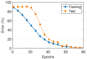
(a)

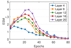
(b)

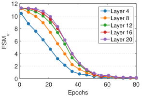
(c)

Figure A1: Experiments with training set $\mathbf{S}$ equaling to the test set $\mathbf{S^{\prime}}$. We follow the same experimental setup as the one in Figure 2 of the paper, except that we use a learning rate of 0.05.

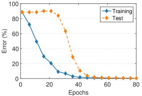
(a)

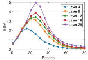
(b)

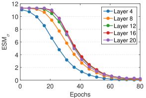
(c)

Figure A2: Experiments with training set $\mathbf{S}$ equaling to the test set $\mathbf{S^{\prime}}$. We follow the same experimental setup as the one in Figure 2 of the paper, except that we use an update factor of $\alpha=0.1$ for the running average in calculate population statistics of BN.

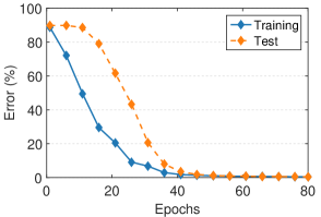
(a)

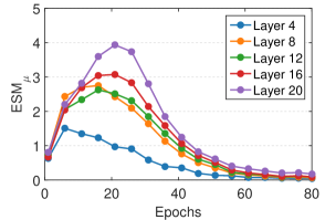
(b)

(c)

Figure A3: Experiments with training set $\mathbf{S}$ equaling to the test set $\mathbf{S^{\prime}}$. We follow the same experimental setup as the one in Figure 2 of the paper, except that we use an update factor of $\alpha=0.5$ for the running average in calculate population statistics of BN.

In Figure 2 of the paper, we show the results of setup one where the training set $\mathbf{S}$ equals to the test set $\mathbf{S^{\prime}}$. The experiments are conducted using a learning rate of 0.1 and an update factor $\alpha=0.9$, trained on the 20-layer multi-layer perceptron (MLP) architecture.

Here, we provide the results under different configurations, including varying the learning rate (Figure A1), varying the update factor $\alpha$ (Figure A2 and A3), varying the depth of the network (Figure A4), and further experiments on convolutional neural networks (Figure A5). We have the similar observations as the ones shown in Figure 2 of the paper: 1) there are significant gaps between the training and test errors in the first dozens of epochs, and these error gaps between training and test are mainly caused by the inaccurate estimation of the population statistics of batch normalization (BN) [17]; 2) the $ESM_{\mu}$ and $ESM_{\sigma}$ of BN in deeper layers have potentially higher values during the first dozens of epochs.

Group normalization with different groups.

In Figure 4 of the paper, we show the results using group normalization (GN) [51] with group number $g=4$. Here, we provide results of GN with group numbers $g=1$ (Figure A6) and $g=16$ (Figure A7). Note that GN with $g=1$ is equivalent to layer normalization (LN) [1]. We have the similar observations as the ones shown in Figure 4 of the paper: 1) the gaps of training and test errors of ‘GNBN’ are significantly reduced in the first 30 epochs; 2) the $ESM_{\sigma}$ of BNs in each layer of ‘GNBN’ nearly are the same during training.

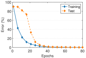
(a)

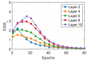
(b)

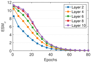
(c)

Figure A4: Experiments with training set $\mathbf{S}$ equaling to the test set $\mathbf{S^{\prime}}$. We follow the same experimental setup as the one in Figure 2 of the paper, except that we train a 10-layer MLP.

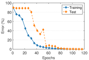
(a)

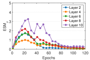
(b)

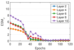
(c)

Figure A5: Experiments with training set $\mathbf{S}$ equaling to the test set $\mathbf{S^{\prime}}$. We train a 14-layer convolutional neural network (CNN) for MNIST classification. $\mathbf{S}$ and $\mathbf{S^{\prime}}$ are the original test set of MNIST with 10,000 samples. We use full-batch gradient descent to train 120 epochs (iterations) with a learning rate of 0.1. The estimated population statistics of BN are calculated by the commonly used running average with update factor $\alpha=0.9$.

Appendix B More Results on ImageNet Classification

In this section, we provide more results on large-scale ImageNet classification [37].

Different group number.

In Section 5.2.1 of the paper, we mention that we use GN with group number $g=64$ as BFN in the XBNBlock. Here, we compare the results between GNs with $g=64$ and $g=32$, under different positions where a GN is used in an XBNBlock. Figure A8 shows the results. We observe that all the models with different group numbers outperform the baseline (BN) significantly. Besides, There are no remarkable differences in performance between the models using GN with $g=64$ and $g=32$.

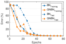
(a)

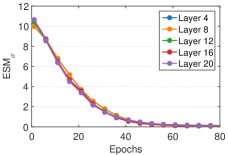
(b)

Figure A6: Estimation shift experiments on a network with BN and GN mixed (referred to as ‘GNBN’). We follow the same experimental setup as the one in Figure 4 of the paper, except that we use GN with a group number of 1.

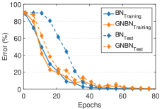
(a)

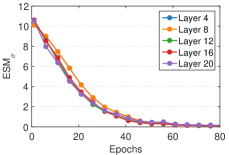
(b)

Figure A7: Estimation shift experiments on a network with BN and GN mixed (referred to as ‘GNBN’). We follow the same experimental setup as the one in Figure 4 of the paper, except that we use GN with a group number of 16.

Figure A8: Comparison of the results (top-1 validation accuracy) between GNs with $g=64$ and $g=32$, under different positions where a GN is used in an XBNBlock. ‘XBNBlock-P1’, ‘XBNBlock-P2’ and ‘XBNBlock-P3’ indicate that the first, second and third BN in the bottleneck are replaced with GN, respectively.

Robustness to distribution shift.

In Figure 8 of the paper, we conduct experiments on model robustness to distribution shift. We show the results on ResNet-50 with its first six blocks being ‘disturbed block’. Here, we provide more results on ResNet-50 with different blocks being ‘disturbed block’, and the results are shown in Figure A9. We obtain similar observations as the ones in Figure 8 of the paper. Besides, we observe that BN has significant performance degeneration, even though only one BN’s population statistics are disturbed (Figure A9 (a)), while XBNBlock_GN and XBNBlock_IN have no remarkable performance degeneration in this case (Figure A9 (a)).

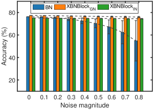
(a)

(b)

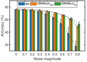
(c)

Figure A9: Top-1 validation accuracy with different noise magnitude imposed on the estimated population statistics. The results are averaged over 5 random seeds. We refer to a bottleneck/XBNBlock as ‘disturbed block’ if its first BN uses $\{\hat{\mu}_{\delta},\hat{\sigma}^{2}_{\delta}\}$ for normalization during inference. (a) the first block of ResNet-50 is ‘disturbed block’; (b) the first 6 blocks of ResNet-50 are ‘disturbed block’; (c) the first 13rd blocks of ResNet-50 are ‘disturbed block’.

Advanced training strategies.

In Section 5.2.2 of the paper, we conduct experiments using more advanced training strategies and show the results on ResNet-50 [9]. Here, we provide the results on ResNet-101 [9] and ResNext-50 [53] (Table A1). We also observe that XBNBlock consistently outperforms the baseline by a remarkable margin.

	ResNet-101		ResNext-50
Training strategies	Baseline (BN)	XBNBlockGN	Baseline (BN)	XBNBlockGN
label smooth (LS)	78.25	78.85	77.83	78.46
MixUp	78.67	79.14	78.20	78.73
cosine learning (COS)	78.51	78.91	77.91	78.31
LS + MixUP + COS	79.10	79.41	78.84	79.27

Table A1: Top-1 accuracy ($\%$) on ResNet-101 and ResNeXt-50 using advanced training strategies.

Towards whitening.

We also apply the recently proposed group whitening (GW) [15] as a BFN in our XBNBlock, referred to as XBNBlock_GW. We use the released code provided in  [15]. The results are shown in Table A2. By applying GW in our design, our XBNBlock outperforms the state-of-the-art whitening methods. E.g., our method ‘XBNBlock_GW-D4’ obtains $79.18\%$ top-1 accuracy on ResNet-101. Note that XBNBlock_GW-D4 has only $7\%$ additional time cost.

Method	ResNet-50	ResNet-101
Baseline (BN) [17]	76.29	77.65
BW [14]	77.21	78.27
SW [34]	77.93	79.13
GW [15]/XBNBlockGW	77.72	78.71
XBNBlockGW-D2 (ours)	77.89	79.12
XBNBlockGW-D4 (ours)	77.56	79.18

Table A2: Comparison of top-1 validation accuracy (%) between methods with whitening module. We compare our method to batch whitening (BW) [14], switchable whitening (SW)  [34] and group whitening (GW)  [15]. Note that the ResNet-50 (ResNet-101) with GW used in paper  [15] is equivalent to the ResNet-50 (ResNet-101) with our XBNBlock_GW used.

Method	Standard training	Advanced training
Baseline (BN)	66.59	70.83
XBNBlockGN	70.81	72.69

Table A3: Top-1 accuracy (%) on MobileNet-V2 for ImageNet classification.

B.1 Experiments on other Architectures

In Section 5.2 of the paper, we show the results experimented on ResNet and ResNeXt architectures. Here, we provide the results on MobileNet-V2 [38] and ShuffleNet-V2 [28] architectures which are designed for more efficient computations. We conduct experiments using XBNBlock-P2 that replace the second BN of the original block of MobileNet-V2 (Figure A10) and ShuffleNet-V2 (Figure A11) with a BFN. We again use GN as BFN.

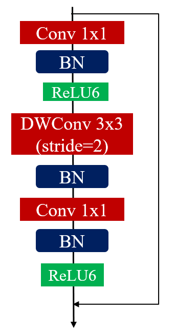
(a)

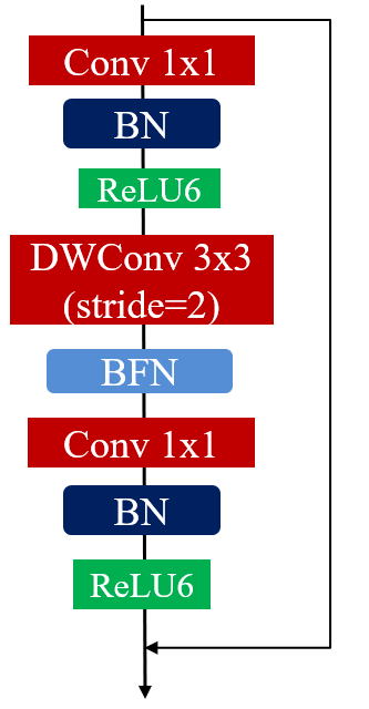
(b)

Figure A10: Inverted residual block of MobileNet-V2 vs our XBNBlock-P2 that replaces its second BN with a BFN. Note that ‘DWconv’ indicates the depth-wise convolutions.

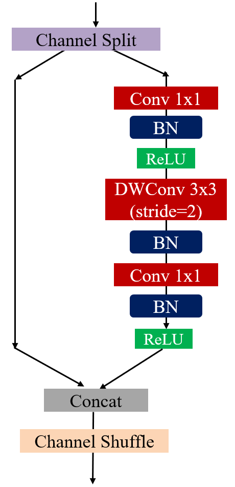
(a)

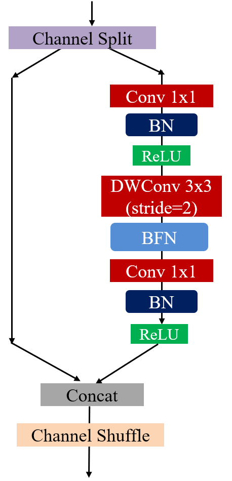
(b)

Figure A11: Basic block of ShuffleNet-V2 vs our XBNBlock-P2 that replaces its second BN with a BFN.

B.1.1 MobileNet-V2

Following the experimental setup shown in the paper, we consider two training protocols:

(1) Standard training protocol: We apply stochastic gradient descent (SGD) using a mini-batch size of 256, momentum of 0.9 and weight decay of 0.0001. We train over 100 epochs. The initial learning rate is set to 0.1 and divided by 10 at 30, 60 and 90 epochs.

(2) Advanced training protocol: We train 150 epochs with cosine learning rate decay, and use a weight decay of 0.00004, under which the baseline model (MobileNet) obtains a better performance.

The results are shown in Table A3. We observe that the proposed XBNBlock consistently improves the performance of the original MobileNet-V2 architecture.

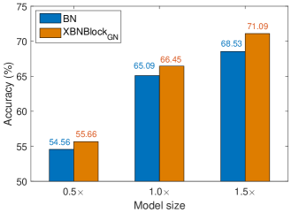
(a)

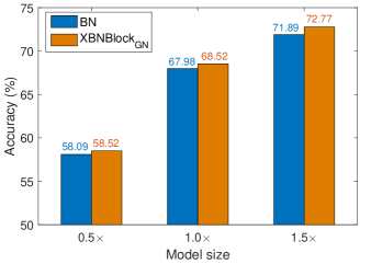
(b)

Figure A12: Top-1 accuracy (%) on ShuffleNet-V2 for ImageNet classification.

B.1.2 ShuffleNet-V2

Here, we also consider two training protocols:

(1) Standard training protocol: We apply SGD using a mini-batch size of 256, momentum of 0.9 and weight decay of 0.0001. We train over 100 epochs. The initial learning rate is set to 0.1 and divided by 10 at 30, 60 and 90 epochs.

(2) Advanced training protocol: We train 150 epochs with cosine learning rate decay, and use a weight decay of 0.00004. We also further use the label smoothing with a smoothing factor of 0.1. The baseline (ShuffleNet-V2) has a better performance under this training protocol.

Table A3 show the results of ShuffleNet-V2 with different model sizes, including the ‘$0.5\times$’, ‘$1.0\times$’ and ‘$1.5\times$’ [28]. We observe that the proposed XBNBlock consistently improve the performance of the original ShuffleNet-V2 architecture, under different training protocols and model sizes.

Appendix C More Results of Detection and Segmentation on COCO

In Section 5.3 the paper, we only report the average precision (AP) for bounding box detection (AP^bbox) and instance segmentation (AP^mask) [25], due to space limit. Here, we report more COCO metrics including the results at different scales (AP₅₀, AP₇₅, AP_s, AP_m and AP_l) for both bounding box detection and instance segmentation. Table A4 and Table A5 show the results using ResNet-50 and ResNeXt-101 respectively as the backbone.

2fc head box
Method	APbbox	AP${}^{bbox}_{50}$	AP${}^{bbox}_{75}$	AP${}^{bbox}_{s}$	AP${}^{bbox}_{m}$	AP${}^{bbox}_{l}$	APmask	AP${}^{mask}_{50}$	AP${}^{mask}_{75}$	AP${}^{mask}_{s}$	AP${}^{mask}_{m}$	AP${}^{mask}_{l}$
$BN^{{\dagger}}$	37.40	59.01	40.43	21.87	40.91	48.17	34.01	55.72	35.9	15.56	37.05	49.86
GN	37.55	59.36	40.87	21.99	40.49	48.43	34.06	55.97	35.76	15.58	36.86	49.61
XBNBlockGN	38.19	60.09	41.65	22.48	41.50	48.73	34.57	56.79	36.58	16.14	37.49	50.58
4conv1fc head box
Method	APbbox	AP${}^{bbox}_{50}$	AP${}^{bbox}_{75}$	AP${}^{bbox}_{s}$	AP${}^{bbox}_{m}$	AP${}^{bbox}_{l}$	APmask	AP${}^{mask}_{50}$	AP${}^{mask}_{75}$	AP${}^{mask}_{s}$	AP${}^{mask}_{m}$	AP${}^{mask}_{l}$
$BN^{{\dagger}}$	37.51	58.26	40.65	21.88	40.72	48.00	33.68	54.90	35.62	15.44	36.60	48.88
GN	39.02	59.87	42.71	23.29	42.14	50.48	34.37	56.56	36.47	15.86	37.16	50.17
XBNBlockGN	39.57	60.64	42.93	24.15	42.32	51.12	34.86	57.06	36.95	17.12	37.41	50.65

Table A4: Detection and segmentation results ($\%$) on COCO using the Mask R-CNN framework implemented in [29]. We use ResNet-50 as the backbone, combined with FPN. All models are trained by 1x lr scheduling (90k iterations), with a batch size of 16 on eight GPUs.

2fc head box
Method	APbbox	AP${}^{bbox}_{50}$	AP${}^{bbox}_{75}$	AP${}^{bbox}_{s}$	AP${}^{bbox}_{m}$	AP${}^{bbox}_{l}$	APmask	AP${}^{mask}_{50}$	AP${}^{mask}_{75}$	AP${}^{mask}_{s}$	AP${}^{mask}_{m}$	AP${}^{mask}_{l}$
$BN^{{\dagger}}$	42.13	63.98	46.35	24.94	45.98	54.87	37.78	60.37	40.34	17.74	40.69	55.43
GN	41.47	63.54	44.76	25.36	45.33	53.20	37.17	60.23	39.31	17.92	40.24	54.12
XBNBlockGN	42.69	64.98	46.20	25.39	46.72	55.03	38.00	61.03	40.39	17.99	40.95	55.52
4conv1fc head box
Method	APbbox	AP${}^{bbox}_{50}$	AP${}^{bbox}_{75}$	AP${}^{bbox}_{s}$	AP${}^{bbox}_{m}$	AP${}^{bbox}_{l}$	APmask	AP${}^{mask}_{50}$	AP${}^{mask}_{75}$	AP${}^{mask}_{s}$	AP${}^{mask}_{m}$	AP${}^{mask}_{l}$
$BN^{{\dagger}}$	42.18	63.22	46.00	25.01	45.60	54.90	37.53	60.18	39.99	17.80	40.49	55.04
GN	42.24	63.00	46.19	25.27	45.76	54.94	37.53	59.82	39.96	18.00	40.42	54.52
XBNBlockGN	43.43	64.56	47.51	25.89	46.65	56.65	38.68	61.62	41.34	18.52	41.60	56.68

Table A5: Detection and segmentation results ($\%$) on COCO using the Mask R-CNN framework and using ResNeXt-101 as the backbone, combined with FPN. All models are trained by 1x lr scheduling (180k iterations), with a batch size of 8 on eight GPUs.

References

- [1] Lei Jimmy Ba, Ryan Kiros, and Geoffrey E. Hinton. Layer normalization. arXiv preprint arXiv:1607.06450, 2016.
- [2] Philipp Benz, Chaoning Zhang, Adil Karjauv, and In So Kweon. Revisiting batch normalization for improving corruption robustness. In WACV, 2021.
- [3] Johan Bjorck, Carla Gomes, and Bart Selman. Understanding batch normalization. In NeurIPS, 2018.
- [4] Andy Brock, Soham De, Samuel L Smith, and Karen Simonyan. High-performance large-scale image recognition without normalization. In ICML, 2021.
- [5] John Bronskill, Jonathan Gordon, James Requeima, Sebastian Nowozin, and Richard E Turner. Tasknorm: Rethinking batch normalization for meta-learning. In ICML, 2020.
- [6] Vitaliy Chiley, Ilya Sharapov, Atli Kosson, Urs Koster, Ryan Reece, Sofia Samaniego de la Fuente, Vishal Subbiah, and Michael James. Online normalization for training neural networks. In NeurIPS, 2019.
- [7] Guillaume Desjardins, Karen Simonyan, Razvan Pascanu, and koray kavukcuoglu. Natural neural networks. In NeurIPS, 2015.
- [8] Kaiming He, Georgia Gkioxari, Piotr Dollár, and Ross B. Girshick. Mask R-CNN. In ICCV, 2017.
- [9] Kaiming He, Xiangyu Zhang, Shaoqing Ren, and Jian Sun. Deep residual learning for image recognition. In CVPR, 2016.
- [10] Tong He, Zhi Zhang, Hang Zhang, Zhongyue Zhang, Junyuan Xie, and Mu Li. Bag of tricks for image classification with convolutional neural networks. In CVPR, 2019.
- [11] Gao Huang, Zhuang Liu, and Kilian Q. Weinberger. Densely connected convolutional networks. In CVPR, 2017.
- [12] Lei Huang, Jie Qin, Yi Zhou, Fan Zhu, Li Liu, and Ling Shao. Normalization techniques in training dnns: Methodology, analysis and application. arXiv preprint arXiv:2009.12836, 2020.
- [13] Lei Huang, Dawei Yang, Bo Lang, and Jia Deng. Decorrelated batch normalization. In CVPR, 2018.
- [14] Lei Huang, Lei Zhao, Yi Zhou, Fan Zhu, Li Liu, and Ling Shao. An investigation into the stochasticity of batch whitening. In CVPR, 2020.
- [15] Lei Huang, Yi Zhou, Li Liu, Fan Zhu, and Ling Shao. Group whitening: Balancing learning efficiency and representational capacity. In CVPR, 2021.
- [16] Sergey Ioffe. Batch renormalization: Towards reducing minibatch dependence in batch-normalized models. In NeurIPS, 2017.
- [17] Sergey Ioffe and Christian Szegedy. Batch normalization: Accelerating deep network training by reducing internal covariate shift. In ICML, 2015.
- [18] Pavel Izmailov, Dmitrii Podoprikhin, Timur Garipov, Dmitry Vetrov, and Andrew Gordon Wilson. Averaging weights leads to wider optima and better generalization. arXiv preprint arXiv:1803.05407, 2018.
- [19] Junho Kim, Minjae Kim, Hyeonwoo Kang, and Kwang Hee Lee. U-gat-it: Unsupervised generative attentional networks with adaptive layer-instance normalization for image-to-image translation. In ICLR, 2020.
- [20] Yann LeCun, Leon Bottou, Genevieve B. Orr, and Klaus-Robert Muller. Efficient backprop. In Neural Networks: Tricks of the Trade, 1998.
- [21] Yann LeCun, Ido Kanter, and Sara A. Solla. Second order properties of error surfaces. In NeurIPS, 1990.
- [22] Boyi Li, Felix Wu, Kilian Q Weinberger, and Serge Belongie. Positional normalization. In NeurIPS, 2019.
- [23] Yanghao Li, Naiyan Wang, Jianping Shi, Jiaying Liu, and Xiaodi Hou. Revisiting batch normalization for practical domain adaptation. arXiv preprint arXiv:1603.04779, 2016.
- [24] Tsung-Yi Lin, Piotr Dollár, Ross B. Girshick, Kaiming He, Bharath Hariharan, and Serge J. Belongie. Feature pyramid networks for object detection. In CVPR, 2017.
- [25] Tsung-Yi Lin, Michael Maire, Serge Belongie, James Hays, Pietro Perona, Deva Ramanan, Piotr Dollár, and C. Lawrence Zitnick. Microsoft coco: Common objects in context. In ECCV, 2014.
- [26] Ilya Loshchilov and Frank Hutter. SGDR: stochastic gradient descent with restarts. In ICLR, 2017.
- [27] Ping Luo, Jiamin Ren, Zhanglin Peng, Ruimao Zhang, and Jingyu Li. Differentiable learning-to-normalize via switchable normalization. In ICLR, 2019.
- [28] Ningning Ma, Xiangyu Zhang, Hai-Tao Zheng, and Jian Sun. Shufflenet v2: Practical guidelines for efficient cnn architecture design. In ECCV, 2018.
- [29] Francisco Massa and Ross Girshick. maskrcnn-benchmark: Fast, modular reference implementation of Instance Segmentation and Object Detection algorithms in PyTorch. https://github.com/facebookresearch/maskrcnn-benchmark, 2018. Accessed: 09-26-2019.
- [30] Grégoire Montavon and Klaus-Robert Müller. Deep Boltzmann Machines and the Centering Trick, volume 7700 of LNCS. Springer, 2nd edn edition, 2012.
- [31] Zachary Nado, Shreyas Padhy, D Sculley, Alexander D’Amour, Balaji Lakshminarayanan, and Jasper Snoek. Evaluating prediction-time batch normalization for robustness under covariate shift. arXiv preprint arXiv:2006.10963, 2020.
- [32] Hyeonseob Nam and Hyo-Eun Kim. Batch-instance normalization for adaptively style-invariant neural networks. In NeurIPS, 2018.
- [33] Xingang Pan, Ping Luo, Jianping Shi, and Xiaoou Tang. Two at once: Enhancing learning and generalization capacities via ibn-net. In ECCV, 2018.
- [34] Xingang Pan, Xiaohang Zhan, Jianping Shi, Xiaoou Tang, and Ping Luo. Switchable whitening for deep representation learning. In ICCV, 2019.
- [35] Adam Paszke, Sam Gross, Soumith Chintala, Gregory Chanan, Edward Yang, Zachary DeVito, Zeming Lin, Alban Desmaison, Luca Antiga, and Adam Lerer. Automatic differentiation in PyTorch. In NeurIPS Autodiff Workshop, 2017.
- [36] Shaoqing Ren, Kaiming He, Ross Girshick, and Jian Sun. Faster R-CNN: Towards real-time object detection with region proposal networks. In NeurIPS, 2015.
- [37] Olga Russakovsky, Jia Deng, Hao Su, Jonathan Krause, Sanjeev Satheesh, Sean Ma, Zhiheng Huang, Andrej Karpathy, Aditya Khosla, Michael Bernstein, Alexander C. Berg, and Li Fei-Fei. ImageNet Large Scale Visual Recognition Challenge. International Journal of Computer Vision (IJCV), 115(3):211–252, 2015.
- [38] Mark Sandler, Andrew G. Howard, Menglong Zhu, Andrey Zhmoginov, and Liang-Chieh Chen. Mobilenetv2: Inverted residuals and linear bottlenecks. In CVPR, 2018.
- [39] Shibani Santurkar, Dimitris Tsipras, Andrew Ilyas, and Aleksander Madry. How does batch normalization help optimization? In NeurIPS, 2018.
- [40] Steffen Schneider, Evgenia Rusak, Luisa Eck, Oliver Bringmann, Wieland Brendel, and Matthias Bethge. Improving robustness against common corruptions by covariate shift adaptation. In NeurIPS, 2020.
- [41] Seonguk Seo, Yumin Suh, Dongwan Kim, Jongwoo Han, and Bohyung Han. Learning to optimize domain specific normalization for domain generalization. In ECCV, 2020.
- [42] Wenqi Shao, Tianjian Meng, Jingyu Li, Ruimao Zhang, Yudian Li, Xiaogang Wang, and Ping Luo. Ssn: Learning sparse switchable normalization via sparsestmax. In CVPR, 2019.
- [43] Sheng Shen, Zhewei Yao, Amir Gholami, Michael W Mahoney, and Kurt Keutzer. Powernorm: Rethinking batch normalization in transformers. In ICML, 2020.
- [44] Saurabh Singh and Abhinav Shrivastava. Evalnorm: Estimating batch normalization statistics for evaluation. In ICCV, 2019.
- [45] Jiaming Song, Yang Song, and Stefano Ermon. Unsupervised out-of-distribution detection with batch normalization. arXiv preprint arXiv:1910.09115, 2019.
- [46] Cecilia Summers and Michael J. Dinneen. Four things everyone should know to improve batch normalization. In ICLR, 2020.
- [47] Christian Szegedy, Sergey Ioffe, and Vincent Vanhoucke. Inception-v4, inception-resnet and the impact of residual connections on learning. In AAAI, 2017.
- [48] Christian Szegedy, Vincent Vanhoucke, Sergey Ioffe, Jonathon Shlens, and Zbigniew Wojna. Rethinking the inception architecture for computer vision. In CVPR, 2016.
- [49] Dmitry Ulyanov, Andrea Vedaldi, and Victor S. Lempitsky. Instance normalization: The missing ingredient for fast stylization. arXiv preprint arXiv:1607.08022, 2016.
- [50] Simon Wiesler and Hermann Ney. A convergence analysis of log-linear training. In NeurIPS, 2011.
- [51] Yuxin Wu and Kaiming He. Group normalization. In ECCV, 2018.
- [52] Yuxin Wu and Justin Johnson. Rethinking ”batch” in batchnorm. arXiv preprint arXiv:2105.07576, 2021.
- [53] Saining Xie, Ross B. Girshick, Piotr Dollár, Zhuowen Tu, and Kaiming He. Aggregated residual transformations for deep neural networks. In CVPR, 2017.
- [54] Junjie Yan, Ruosi Wan, Xiangyu Zhang, Wei Zhang, Yichen Wei, and Jian Sun. Towards stabilizing batch statistics in backward propagation of batch normalization. In ICLR, 2020.
- [55] Zhuliang Yao, Yue Cao, Shuxin Zheng, Gao Huang, and Stephen Lin. Cross-iteration batch normalization. In CVPR, 2021.
- [56] Hongwei Yong, Jianqiang Huang, Xiansheng Hua, and Lei Zhang. Gradient centralization: A new optimization technique for deep neural networks. In ECCV, 2020.
- [57] Sergey Zagoruyko and Nikos Komodakis. Wide residual networks. In BMVC, 2016.
- [58] Hongyi Zhang, Moustapha Cisse, Yann N. Dauphin, and David Lopez-Paz. mixup: Beyond empirical risk minimization. In ICLR, 2018.
- [59] Ruimao Zhang, Zhanglin Peng, Lingyun Wu, Zhen Li, and Ping Luo. Exemplar normalization for learning deep representation. In CVPR, 2020.