Graph Convolutional Neural Networks Sensitivity under Probabilistic Error Model

Abstract

Graph Neural Networks (GNNs), particularly Graph Convolutional Networks (GCNs), have emerged as pivotal instruments in machine learning and signal processing for processing graph-structured data. This paper presents a thorough investigation of the sensitivity and robustness of GCNs, an important class of GNNs, under graph perturbations. We concentrate on the perturbed graph shift operator (GSO) and propose a sensitivity analysis framework based on it. The results yield explicit analytical expressions for error bounds and unveil a linear inequality relationship between the output variances of the original and perturbed GCNs and the GSO error. The proposed approach for probabilistic error model in GSO is also extended to two popular GCN variants, namely, Graph Isomorphism Network (GIN) and Simple Graph Convolution Network (SGCN). Extensive experiments provide empirical validation of the theoretical derivations, underlining our approach’s efficacy in discerning the stability performance of GCNs. Ultimately, our work provides insights into the effects of structural perturbations on graph-structured data processing, thus fostering the evolution of more resilient GNN architectures.

I Introduction

Graph neural networks have steadily gained prominence as an innovative instrument in machine learning and signal processing, exhibiting unparalleled efficiency in processing data encapsulated within complex graph structures [1, 2, 3]. Uniquely designed, GNNs utilize a system of intricately coupled graph filters with nonlinear activation functions, enabling the effective transformation and propagation of information within the graph [4, 5].

Different GNN architectures can be delineated based on the graph filters (GFs) that they use, which is an integral component for the functioning of GNNs. A notable example of these architectures uses graph-convolutional filters. The GNN employing this design is known as the Graph Convolutional Network (GCN). Some notable examples of GCNs include the vanilla GCN [6], Graph Isomorphism Network (GIN) [6], Simple Graph Convolution Network (SGCN) [7, 8], and Cayley Graph Convolutional Network (CayleyNet) [9]. In contrast to the aforementioned GCNs, there exist non-convolutional GNNs such as the Graph Attention Network (GAT) [10] and Edge Varying Graph Neural Network (EdgeNet) [11], which utilize edge-varying graph filters [12].

This paper delves into the GCN, which blends graph convolutional filters with nonlinear activation functions. Graph convolutional filters couple the data and graph with the underlying graph matrix, named graph shift operator (GSO), which can be, for example, the graph adjacency matrix or graph Laplacian, which encodes the interactions between data samples [13]. Based on the GSO, the graph filter captures the structural information by aggregating the data propagated within its $k-$hop neighborhoods, and feeds it to the next layer after processing, which can be applying graph coarsening and pooling [14, 15]. As the key component of GCNs, GSO presents the graph structure, and is typically assumed to be perfectly known. The precise estimation of the hidden graph structure is essential for successfully performing feature propagation in a convolution layer [16, 17, 18].

GSOs form the foundation of GCN structures, establishing the complex interactions between nodes and influencing the propagation of signals across the network. Therefore, any perturbation in the graph structure has a direct bearing on the operations of a GCN. Modeling and processing under deterministic and stochastic perturbations on GSOs have been performed in the existing literature on graph signal processing (GSP) and GNN. A probabilistic graph error model for a partially correct estimation of the adjacency matrix is proposed in [19], where a perturbed graph is modeled as a combination of the true adjacency matrix and a perturbation term specified by Erdös-Rényi (ER) graph. In [20], a graph error model is constructed by successively connecting two nodes that are not connected to study the relation between algebraic connectivity with an increasing number of edges. Complementarily, [21] discusses the strategy of rewiring edge selection for the most significant increase in algebraic connectivity. With increased connectivity, the network is more robust against attacks and failures. In [22], a GSO perturbation strategy is formulated leveraging a general first-order optimization method, which concurrently imposes a constraint on the extent of edge perturbation. In [23], closed-form expressions of perturbed eigenvector pairs under edge perturbation are derived using small perturbation analysis, and signal processing algorithms that are robust to graph errors are given. The work [24] explores errors in graphs using random edge sampling, a scheme characterized by the stochastic deletion of existing edges.

The robustness of a GCN under perturbations in GSOs gives rise to a more nuanced perspective on the network’s resilience. In [25], a comprehensive stability bound for GCN within a semi-supervised framework is presented. The authors highlight the correlation between the algorithmic stability of a GCN and the maximum absolute eigenvalue of its graph convolution filter. The impact of generic graph perturbations on GNN performance is scrutinized in [26], where the authors establish the stability of GCNs featuring integral Lipschitz filters under relative graph perturbations. They further derive an analytical upper bound, controlled by the operator norm of the error matrix. The scope for improvement arises due to the general graph error model utilized, suggesting potential enhancements through specification of the error model and network architecture. Continuing along the analytical framework, [26] and [27] offer an in-depth analysis of the GCN’s robustness under slight perturbations including modifications in translation-invariant kernels, node distributions, and graph signal alterations within the context of a large random graph. The work [28] explores the concept of robustness certificates for GCN graph perturbations. By limiting the number of non-zero elements in the adjacency matrix, the authors present a nuanced perspective on the network’s resilience.

Somewhat contradictory stability results have been reported between the signal processing (SP) and computer science (CS) communities. In SP, the works [26, 24, 29] suggest that GCNs maintain stability under perturbations, provided that the perturbation budget is constrained. On the contrary, in CS, research such as [30, 31, 32, 33] has pointed to vulnerabilities of GCN models to adversarial attacks on graphs. These vulnerabilities, despite the models’ effectiveness in graph learning tasks, have been empirically demonstrated through experiments involving edge dropping and adversarial training. These contrasting perspectives on GCN stability call for a fresh approach. In response, this paper introduces a sensitivity analysis framework specifically designed to address perturbations on the GSO and, subsequently, on GCNs. To demonstrate the utility and adaptability of this framework, we apply it to an error model well received within the SP community [19], that is based on the probabilistic Erdös-Rényi model to specify the GSO error. Furthermore, to specify the GCN output, we incorporate GIN and SGCN with two different GSOs. These GSOs’ sensitivity, analyzed within our proposed framework, further substantiates the effectiveness of our methodology.

We aim to develop a generic sensitivity analysis framework for GCNs to reconcile the aforementioned discrepancies, taking into account the varying error types or models. Our detailed contributions are listed as follows.

1. Proposal of a Generic Framework: The principal contribution is the development of a generic GCN sensitivity analysis framework for GSO perturbations. Although the currently used error model does not encapsulate all forms of adversarial attacks, it paves the way for the integration of these attacks as statistical models in future studies. Our framework introduces a comprehensive approach to understanding contradictory results in stability and enhances the development of robust and reliable GCN models.

2. Analysis of GSO Error Model: We employ a well-accepted GSO error model to derive

   • Analytical expressions for the error of the GSO using the $\ell_{1}$ norm, which is closely linked to node degree alteration. This provides valuable insights into the impact of structural perturbations on the graph.

   • Analytical expressions for error bounds that highlight the GSO’s resilience, an element crucial to both GFs and GCNs.

3. Empirical Validation: We have conducted an in-depth examination of the GF and GCN performance under perturbations, providing detailed analytical expressions for their respective error bounds. Our analysis concentrates on two widely used GCN variants, GIN and SGCN, which utilize an augmented adjacency matrix and a normalized adjacency matrix, respectively. We have shown empirically a linear inequality relationship between the output difference of the original and perturbed GCNs and the GSO error, which is in parallel with the theoretical result. This study illustrates that any variation in the GCN output due to the perturbed graph can be bounded linearly, even without explicit knowledge of the perturbed graph’s structure. The numerical results obtained from our comprehensive experiments confirm our theoretical derivations, thereby substantiating our sensitivity analysis model’s reliability.

The structure of the remainder of this paper is as follows. In Sections II and III, we establish the fundamentals of GCNs and proceed to formulate the problem under examination, respectively. In Section IV, we conduct an exhaustive analytical study on the sensitivity of GSO to probabilistic graph perturbations, with particular emphasis on two cases: the graph adjacency matrix and its normalized version. Following the GSO sensitivity analysis, Section V explores and establishes the linearity between the GCN output difference and the GSO distance for both GF and two GCN variants, SGCN and GIN. Subsequently, we utilize the numerical experiments conducted in Section VI to validate and corroborate the theorems we propose. Finally, Section VII concludes the paper.

Notation. Boldface lower case letters such as ${\mathbf{x}}$ represent column vectors, while boldface capital letters like ${\mathbf{X}}$ denote matrices. A vector full of ones is symbolized as $\mathbf{1}_{N}$, and a $N\times N$ matrix full of ones is expressed as $\mathbf{1}_{N\times N}=\mathbf{1}_{N}\mathbf{1}_{N}^{\top}$. The identity matrix of size $N\times N$ is represented as ${\mathbf{I}}_{N\times N}$. The $i$-th row or column of the matrix ${\mathbf{A}}$ is given as ${\mathbf{A}}_{i}$, and the $(i,j)$-th element in matrix ${\mathbf{A}}$ is denoted as $[{\mathbf{A}}]_{i,j}$. Matrix norms are defined as follows: the $\ell_{1}$ norm is represented as $\|{\mathbf{A}}\|_{1}=\max_{i}\sum_{j}|{\mathbf{A}}_{i,j}|$, the $\ell_{2}$ norm as $\|{\mathbf{A}}\|=\|{\mathbf{A}}\|_{2}$, the $\ell_{\infty}$ norm as $\|{\mathbf{A}}\|_{\infty}=\max_{j}\sum_{i}|{\mathbf{A}}_{i,j}|$. In addition , the Hadamard product is expressed with the symbol $\circ$. We use $\textrm{Pr}(\cdot)$ for probability, ${\mathbb{E}}(\cdot)$ for expectation, $\mathrm{Var}(\cdot)$ for variance, and $\text{Cov}(\cdot,\cdot)$ for covariance.

II Preliminaries

Graph theory, GSP, and GCN form the cornerstone of data analysis in irregular domains. The GSO in particular plays a key role in directing information flow across the graph, thereby enabling the creation of GFs and the design of GNNs.

The stability analysis of the GSO, which essentially involves matrix sensitivity analysis, provides an empirical insight into the system’s resilience to perturbations. The GCN, with its local architecture, maintains most of the properties of the graph convolutional filter, making it an ideal tool for stability analysis. These preliminary concepts are essential for the implementation of stability analysis in a graph-based context.

Graph basics. Consider an undirected and unweighted graph ${\mathcal{G}}=({\mathcal{V}},{\mathcal{E}},{\mathcal{W}})$, where the node set ${\mathcal{V}}=\{1,\ldots,N\}$ consists of $N$ nodes, the edge set ${\mathcal{E}}$ is a subset of ${\mathcal{V}}\times{\mathcal{V}}$, and the edge weighting function ${\mathcal{W}}:{\mathcal{E}}\to\{0,1\}$ assigns binary edges. For an edge $(i,j)\in{\mathcal{E}}$, we have ${\mathcal{W}}(i,j)={\mathcal{W}}(j,i)=1$ due to our focus on undirected and unweighted graphs. We define the $1$-hop neighboring set of a node $i$ as ${\mathcal{N}}_{i}=\{j\in{\mathcal{V}}:(i,j)\in{\mathcal{E}}\}$, the degree of node $i$ as $d_{i}$, and the minimum degree of nodes around $i$ as $\tau_{i}=\min_{j\in{\mathcal{N}}_{i}}d_{j}$.

GSO. The Graph Shift Operator (GSO) ${\mathbf{S}}\in{\mathbb{R}}^{N\times N}$ symbolizes the structure of a graph and guides the passage and fusion of signals between neighboring nodes. It is often represented by the adjacency matrix ${\mathbf{A}}$, the Laplacian ${\mathbf{L}}$, or their normalized counterparts. These representations capture the graph’s connectivity patterns, marking them indispensable tools for data analysis in both regular and irregular domains [34]. The adjacency matrix, denoted by ${\mathbf{A}}$, incorporates both the weighting function and the graph topology ${\mathcal{G}}$, where $[{\mathbf{A}}]_{ij}=1$ if $(i,j)\in{\mathcal{E}}$ and $[{\mathbf{A}}]_{ij}=0$ if $(i,j)\not\in{\mathcal{E}}$. The Laplacian matrix ${\mathbf{L}}$ is defined by the adjacency matrix and a diagonal degree matrix ${\mathbf{D}}$. Specifically, ${\mathbf{L}}={\mathbf{D}}-{\mathbf{A}}$, where ${\mathbf{D}}=\text{diag}({\mathbf{A}}{\mathbf{1}}_{N})$ is a diagonal matrix, and $[{\mathbf{D}}]_{ii}=d_{i}$. The value $d_{i}=\sum_{j\in{\mathcal{N}}_{i}}[{\mathbf{A}}]_{ij}$ denotes the degree of node $i$. Moreover, normalized versions of the adjacency and Laplacian matrices are defined as ${\mathbf{A}}_{\textrm{n}}={\mathbf{D}}^{-1/2}{\mathbf{A}}{\mathbf{D}}^{-1/2}$ and ${\mathbf{L}}_{\textrm{n}}={\mathbf{D}}^{-1/2}{\mathbf{L}}{\mathbf{D}}^{-1/2}$, respectively. These normalized versions help maintain consistency and manage potential variations in the scale of the data.

Graph Convolutional Filter. Using GSO, graph signals undergo shifting and averaging across their neighboring nodes. The signal on the graph is denoted by ${\mathbf{x}}\in{\mathbb{R}}^{N}$. Its $i$-th entry $[{\mathbf{x}}]_{i}=x_{i}$ specifies the data value at the node $v_{i}$. The one time shift of graph signal is simply ${\mathbf{S}}{\mathbf{x}}$, whose value at node $i$ is $[{\mathbf{S}}{\mathbf{x}}]_{i}=\sum_{j\in{\mathcal{N}}_{i}}s_{ij}x_{j}$. After one graph shift, the value at node $i$ is given by moving a local linear operator over its neighborhood values $\{x_{j}\}_{j\in{\mathcal{N}}}$. Based on the graph shifting, a graph convolutional filter ${\mathbf{h}}({\mathbf{S}})$ with $K$ taps is defined via polynomials of GSO and the filter weights ${\mathbf{h}}=\{h_{k}\}_{k=0}^{K}$ in the graph convolution

$${\mathbf{y}}=h_{0}{\mathbf{S}}^{0}{\mathbf{x}}+\cdots+h_{K}{\mathbf{S}}^{K}{\mathbf{x}}=\sum_{k=0}^{K}h_{k}{\mathbf{S}}^{k}{\mathbf{x}}={\mathbf{H}}({\mathbf{S}}){\mathbf{x}},$$ (1)

where ${\mathbf{y}}$ is the filter’s output and ${\mathbf{H}}({\mathbf{S}})=\sum_{k=0}^{K}h_{k}{\mathbf{S}}^{k}$ is a shift-invariant graph filter with $K$ taps, and denotes the weight of local information after $K$-hop data exchanges. These filters are then stacked with nonlinearities, forming the primary components of a GCN. GCNs extend this concept by stacking layers of graph convolutional filters followed by nonlinearities.

Graph Perceptron and GCN. A Graph Perceptron [35] is a simple unit of transformation in the GCN. The functionality of a graph perceptron can be seamlessly extended to accommodate graph signals with multiple features. Specifically, a multi-feature graph signal can be denoted by ${\mathbf{X}}=[{\mathbf{x}}_{1},\cdots,{\mathbf{x}}_{d}]\in{\mathbb{R}}^{N\times d}$, where $d$ signifies the number of features. The architecture of an $L$-layer GCN is built upon cascading multiple graph perceptrons. It operates such that the output of a graph perceptron in a preceding layer serves as the input to the graph perceptron at the subsequent layer $\ell$, where $\ell$ spans from $1$ to $L$. We denote the feature fed to the first layer as ${\mathbf{X}}_{0}={\mathbf{X}}$. For an $L$-layer GCN, the graph perceptron at layer $\ell$ can be represented as

$$\begin{split}{\mathbf{Y}}_{\ell}=\sum_{k=1}^{K}{\mathbf{S}}^{k}{\mathbf{X}}_{\ell-1}{\mathbf{H}}_{\ell k},\ \ {\mathbf{X}}_{\ell}=\sigma_{\ell}\left({\mathbf{Y}}_{\ell}\right),\end{split}$$ (2)

Here, ${\mathbf{Y}}_{\ell}$ signifies the intermediate graph filter output, $\sigma_{\ell}(\cdot)$ denotes the nonlinear activation function at layer $\ell$, and graph signals at each layer are ${\mathbf{X}}_{\ell}$ and ${\mathbf{X}}_{\ell-1}$ with sizes of ${\mathbb{R}}^{N\times F_{\ell}}$ and ${\mathbb{R}}^{N\times F_{\ell-1}}$, respectively, where $F_{\ell}$ denotes the number of features at the $\ell$-th layer. The bank of filter coefficients is represented by ${\mathbf{H}}=\{{\mathbf{H}}_{\ell k}\}_{\ell=1,\ldots,L;k=1,\ldots,K}$. By recursively using equation (2) until $\ell=L$, a general GCN can be formulated as:

$$\boldsymbol{\Phi}({\mathbf{X}};{\mathbf{H}},{\mathbf{S}})={\mathbf{X}}_{L}.$$ (3)

This hierarchical arrangement facilitates the flow of information through successive layers, thus enabling effective learning from graph-structured data. Several variations of GCNs have nuances in their specific forms of graph convolution and nonlinearity. Given the intermediate graph filter output ${\mathbf{Y}}_{\ell}$, and the graph signals in each layer, ${\mathbf{X}}_{\ell}$ and ${\mathbf{X}}_{\ell-1}$, we denote ${\mathbf{X}}_{\ell}=\sigma({\mathbf{Y}}_{\ell})$. Therefore, the operation of a general GCN can be defined as a sequence of operations applied recursively over each layer until we reach the final layer $L$. This can be expressed as

$$\boldsymbol{\Phi}({\mathbf{X}};{\mathbf{H}},{\mathbf{S}})={\mathbf{X}}_{L}=\sigma({\mathbf{S}}{\mathbf{X}}_{L-1}{\mathbf{H}}_{Lk}).$$ (4)

This representation captures the recursive nature of GCN operations, going through each layer and applying the corresponding transformation defined by the graph signal, filter coefficients, and non-linearity function. It also directly ties the GCN output to the final layer’s graph signal.

III Problem Formulation

A pivotal aspect of understanding the stability of a GCN is the consideration of potential alterations in the underlying graph structure. These alterations can be broadly construed as perturbations to the GSO, intrinsically linking to changes in the graph topology. In the simplest form, any perturbation to the GSO can be depicted as

$${\hat{\mathbf{S}}}={\mathbf{S}}+{\mathbf{E}},$$ (5)

where ${\hat{\mathbf{S}}}$ signifies the perturbed GSO, ${\mathbf{S}}$ is the original GSO, and ${\mathbf{E}}$ represents the error term. The spectral norm of this error term is denoted by

$$d({\hat{\mathbf{S}}},{\mathbf{S}})=\|{\hat{\mathbf{S}}}-{\mathbf{S}}\|=\|{\mathbf{E}}\|.$$ (6)

Inspired by a previous work [19], we utilize a stochastic error model to represent graph perturbations, where each edge of the graph is subject to perturbation independently. In this context, we primarily focus on the alterations occurring within the neighborhood of a particular node $u\in{\mathcal{V}}$. More specifically, the perturbed neighborhood may encompass additional nodes (${\mathcal{A}}_{u}$), deleted nodes (${\mathcal{D}}_{u}$), and remaining nodes (${\mathcal{R}}_{u}$), which ultimately leads to changes in node degree and modifications to the adjacency matrix. We aim to quantify the sensitivity of GSO in relation to these perturbations. To this end, we adopt and expand upon the notation used in [29, 36] for clarity and consistency.

When the graph undergoes perturbations, it transforms into $\hat{{\mathcal{G}}}=({\mathcal{V}},\hat{{\mathcal{E}}},\hat{{\mathcal{W}}})$, with the node set remaining unaffected. We express degrees of node $u\in{\mathcal{V}}$ in original and perturbed graphs as $d_{u}=\sum_{j}|[{\mathbf{A}}_{u}]_{j}|$ and ${\hat{d}}_{u}=\sum_{j}|{\hat{\mathbf{A}}}_{u,j}|=d_{u}+\delta_{u}$, respectively. Here, ${\hat{\mathbf{A}}}$ denotes the adjacency matrix of the perturbed graph $\hat{{\mathcal{G}}}$, and $\delta_{u}=\delta_{u}^{+}-\delta_{u}^{-}$ is the degree change at node $u$, with $\delta_{u}^{+}=|{\mathcal{A}}_{u}|$ and $\delta_{u}^{-}=|{\mathcal{D}}_{u}|$ corresponding to the number of edges added and deleted, respectively. We will further delve into the assumptions for the error model and its effects on the GCN’s performance in the following discussion.

III-A Probabilistic Graph Error Model

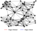
(a) $\epsilon_{1}=0,\epsilon_{2}=0$

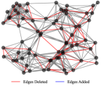
(b) $\epsilon_{1}=0.3,\epsilon_{2}=0$

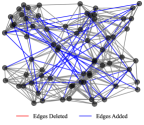
(c) $\epsilon_{1}=0,\epsilon_{2}=0.1$

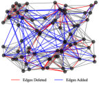
(d) $\epsilon_{1}=0.3,\epsilon_{2}=0.1$

Figure 1: Visual representation of the probabilistic graph error model applied to a random geometric graph. From left to right: (a) Original graph; (b) Graph after edge deletions ($\epsilon_{1}=0.3,\epsilon_{2}=0$); (c) Graph after edge additions ($\epsilon_{1}=0,\epsilon_{2}=0.1$); (d) Graph after both edge deletions and additions ($\epsilon_{1}=0.3,\epsilon_{2}=0.1$). Deleted edges are marked in red and added edges are marked in blue. The transformations effectively illustrate the impact of perturbations modeled by (7).

In this work, we utilize an Erdös-Rényi (ER) graph-based model for perturbations on a graph adjacency matrix, following the approach proposed in [19]. The adjacency matrix of an ER graph is characterized by a random $N\times N$ matrix $\mathbf{\Delta}_{\epsilon}$, where each element of the matrix is generated independently, satisfying $\textrm{Pr}([\mathbf{\Delta}_{\epsilon}]_{i,j}=1)=\epsilon$ and $\textrm{Pr}([\mathbf{\Delta}_{\epsilon}]_{i,j}=0)=1-\epsilon$ for all $i\neq j$. The diagonal elements are zero, i.e., $[\mathbf{\Delta}_{\epsilon}]_{i,i}=0$ for $i=1,\dots,N$, eliminating the possibility of self-loops. For the sake of our analysis, we also assume that the perturbed graph $\hat{{\mathcal{G}}}$ does not contain any isolated nodes, meaning that for all $u\in\hat{{\mathcal{V}}}$, ${\hat{d}}_{u}\geq 1$. For undirected graphs, the model can be adapted by employing the lower triangular matrix $\boldsymbol{\Delta}_{\epsilon}^{l}$, and then defining $\boldsymbol{\Delta}_{\epsilon}=\boldsymbol{\Delta}_{\epsilon}^{l}+(\boldsymbol{\Delta}_{\epsilon}^{l})^{\top}$. Consequently, by specifying the error term in (5), the perturbed adjacency matrix of a graph signal can be expressed as

$${\hat{\mathbf{A}}}={\mathbf{A}}-\boldsymbol{\Delta}_{\epsilon_{1}}\circ{\mathbf{A}}+\boldsymbol{\Delta}_{\epsilon_{2}}\circ(\mathbf{1}_{N\times N}-{\mathbf{A}}),$$ (7)

where the first term is responsible for edge removal with probability $\epsilon_{1}$, and the second term accounts for edge addition with probability $\epsilon_{2}$. This error model can be conceptualized as superimposing two ER graphs on top of the original graph. To better illustrate this model, we utilize visual aids based on a random geometric graph [37, 38]. Fig. 1 visually represents the transition from the original graph to perturbed versions, which include the graph with only edge deletions ($\epsilon_{1}=0.3,\epsilon_{2}=0$), the graph with only edge additions ($\epsilon_{1}=0,\epsilon_{2}=0.1$), and the graph with both edge deletions and additions ($\epsilon_{1}=0.3,\epsilon_{2}=0.1$). Each state depicts the progressive impacts of the perturbations.

In this context, the impact of the perturbation on the degree of a given node $u\in{\mathcal{V}}$ can be computed as follows. The effect of edge deletion is represented by $(-\boldsymbol{\Delta}_{\epsilon_{1}}\circ{\mathbf{A}})_{u}$, where each non-zero element in ${\mathbf{A}}_{u}$ has a probability of $\epsilon_{1}$ being deleted. Thus, the total number of deleted edges $\delta_{u}^{-}$ is the sum of $d_{u}$ independent and identically distributed (i.i.d.) Bernoulli random variables, each with a probability of $\epsilon_{1}$. Similarly, the effect of edge addition is denoted by $\left(\boldsymbol{\Delta}_{\epsilon_{2}}\circ(\mathbf{1}_{N\times N}-{\mathbf{A}})\right)_{u}$, and the total number of added edges $\delta_{u}^{+}$ is the sum of $d_{u}^{*}$ i.i.d. Bernoulli random variables, each with a probability of $\epsilon_{2}$, where $d_{u}^{*}=N-d_{u}-1$. Hence, we can express the number of deleted edges $\delta_{u}^{-}$ and the number of added edges $\delta_{u}^{+}$ as following binomial distributions:

$$\begin{split}\delta_{u}^{-}\sim\textrm{Bin}(d_{u},\epsilon_{1}),\ \delta_{u}^{+}\sim\textrm{Bin}(d_{u}^{*},\epsilon_{2}),\end{split}$$ (8)

where $\textrm{Bin}(n,p)$ represents a binomial distribution with parameters $n$ and $p$.

IV GSO Sensitivity

IV-A Error Bound for Unnormalized GSO Using $\ell_{1}$ Norm

Building on the foundation laid by the discussion of graph structure perturbations and the proposed error model, we now outline the primary theoretical contributions of this study. Our focus here is to detail the probabilistic bounds that help quantify the sensitivity of the GSO to graph structure perturbations. We examine the case where the adjacency matrix serves as the GSO, implying ${\hat{\mathbf{S}}}={\hat{\mathbf{A}}}$ and ${\mathbf{S}}={\mathbf{A}}$. The error model derived in (7) can be expressed as

$${\mathbf{E}}={\hat{\mathbf{A}}}-{\mathbf{A}}=-\boldsymbol{\Delta}_{\epsilon_{1}}\circ{\mathbf{A}}+\boldsymbol{\Delta}_{\epsilon_{2}}\circ(\mathbf{1}_{N\times N}-{\mathbf{A}}).$$ (9)

We can link the change in degree with the $\ell_{1}$ norm of error term in (9) as

$$\|{\mathbf{E}}\|_{1}=\max_{u\in{\mathcal{V}}}\|{\mathbf{E}}_{u}\|_{1},$$ (10)

where

$$\begin{split}\|{\mathbf{E}}_{u}\|_{1}=|{\mathcal{D}}_{u}|+|{\mathcal{A}}_{u}|=\delta_{u}^{-}+\delta_{u}^{+}.\end{split}$$ (11)

Let $Y_{u}=\delta_{u}^{-}+\delta_{u}^{+},u\in{\mathcal{V}}$ and $Y\triangleq\max_{u\in{\mathcal{V}}}Y_{u}$. Since $\delta_{u}^{-}$ and $\delta_{u}^{+}$ are independent random variables, it is not appropriate to give deterministic upper bounds. Instead, we present expected value bounds, which are better suited for analyzing the degree changes of nodes given the probabilistic nature of the model. Our goal is to derive a closed-form expression for the expectation of the maximum node degree error, i.e.,

$${\mathbb{E}}[\|{\mathbf{E}}\|_{1}]={\mathbb{E}}[\max_{u\in{\mathcal{V}}}\|{\mathbf{E}}_{u}\|_{1}].$$ (12)

The probability mass function (PMF) of $Y_{u}$ can be found by convolving the PMFs of $\delta_{u}^{-}$ and $\delta_{u}^{+}$, which are independent random variables. Following binomial distributions in (8), we can obtain the following PMFs

$$\text{Pr}_{\delta_{u}^{-}}(k) =\begin{pmatrix}d_{u}\\ k\end{pmatrix}\epsilon_{1}^{k}(1-\epsilon_{1})^{d_{u}-k},\ k=0,\ldots,d_{u},$$ (13)

$$\text{Pr}_{\delta_{u}^{+}}(k) =\begin{pmatrix}d_{u}^{*}\\ k\end{pmatrix}\epsilon_{2}^{k}(1-\epsilon_{2})^{d_{u}^{*}-k},\ k=0,\ldots,d_{u}^{*},$$ (14)

where $d_{u}^{*}=N-d_{u}-1$, $\text{Pr}_{\delta_{u}^{-}}(k)$ and $\text{Pr}_{\delta_{u}^{+}}(k)$ represent the probabilities of $\delta_{u}^{-}$ and $\delta_{u}^{+}$ taking the value $k$, respectively. Then, the PMF of $Y_{u}$ can be computed as

$$\begin{split}\text{Pr}_{Y_{u}}(k)&=\sum_{i=\max\{0,k-d_{u}^{*}\}}^{\min\{k,d_{u}\}}\text{Pr}_{\delta_{u}^{-},\delta_{u}^{+}}(i,k-i)\\ &=\sum_{i=\max\{0,k-d_{u}^{*}\}}^{\min\{k,d_{u}\}}\text{Pr}_{\delta_{u}^{-}}(i)\text{Pr}_{\delta_{u}^{+}}(k-i)\end{split}$$ (15)

where $k=0,...,N-1$. Using (15), the cumulative distribution function (CDF) of $Y$ is computed as

$$\text{F}_{Y}(k)=\text{Pr}(Y\leq k)=\text{Pr}(\max(Y_{1},\ldots,Y_{N})\leq k)$$

$$=\text{Pr}(Y_{1}\leq k,\ldots,Y_{N}\leq k)=\prod_{u=1}^{N}\text{Pr}(Y_{u}\leq k).$$

Given that $Y_{u}$ for $u\in{\mathcal{V}}$ are i.i.d. and for $k=1,\ldots,N-1$, the CDFs for $Y$ and $Y_{u}$ are as follows

$$\text{F}_{Y}(k)=\prod_{u=1}^{N}\text{F}_{Y_{u}}(k),\quad\text{F}_{Y_{u}}(k)=\sum_{j=0}^{k}\text{Pr}_{Y_{u}}(j).$$ (16)

With the PMF of $Y$ taking on a specific value $k$ being $\text{Pr}_{Y}(k)=\text{F}_{Y}(k)-\text{F}_{Y}(k-1)$, the expectation of $Y$ can be represented as

$${\mathbb{E}}[Y] =\sum_{k=1}^{N-1}k\text{Pr}_{Y}(k)=\sum_{k=1}^{N-1}k\left[\text{F}_{Y}(k)-\text{F}_{Y}(k-1)\right]$$ (17)

which provides a closed-form expression for ${\mathbb{E}}[Y]={\mathbb{E}}[\|{\mathbf{E}}\|_{1}]$. The variance of $Y$ can also be given as

$$\mathrm{Var}[Y]=\mathrm{Var}[\|{\mathbf{E}}\|_{1}]={\mathbb{E}}[Y^{2}]-({\mathbb{E}}[Y])^{2},$$ (18)

where ${\mathbb{E}}[Y^{2}]=\sum_{k=1}^{N-1}k^{2}\text{Pr}_{Y}(k)$.

IV-B Bridging $\ell_{1}$ and $\ell_{2}$ Norms in GSO Analysis

In the analysis of graph-structured data, the spectral norm ($\ell_{2}$ norm), is often employed to quantify the graph spectral error. While [39] did furnish a spectral error bound for the GSO, the need for a more refined and interpretable bound persists to enable more comprehensive analyses. Following the approach of [36], this study utilizes the $\ell_{1}$ norm. The proposed approach of bounding $\|{\mathbf{E}}\|$ is based on assumptions of an undirected graph and perturbation ${\mathbf{E}}={\mathbf{E}}^{\top}$. Using inequalities $\|{\mathbf{E}}\|^{2}\leq\|{\mathbf{E}}\|_{1}\|{\mathbf{E}}\|_{\infty}$ and the fact in our case $\|{\mathbf{E}}\|_{1}=\|{\mathbf{E}}\|_{\infty}$, the $\ell_{2}$ norm can be bounded by the $\ell_{1}$ norm

$$\|{\mathbf{E}}\|\leq\|{\mathbf{E}}\|_{1}=\max_{u\in{\mathcal{V}}}\|{\mathbf{E}}_{u}\|_{1}.$$ (19)

The entries in the error matrix ${\mathbf{E}}$ of equation (9) are random variables. As such, it is challenging to derive a deterministic bound for (19) that is both tight and generalizable. In contrast, an expected bound

$${\mathbb{E}}[\|{\mathbf{E}}\|]\leq{\mathbb{E}}[\|{\mathbf{E}}\|_{1}]={\mathbb{E}}[\max_{u\in{\mathcal{V}}}\|{\mathbf{E}}_{u}\|_{1}],$$ (20)

provides a more reasonable estimate of the true behavior of the error matrix, as it takes into account the distribution of the random variables, as well as the structural changes of the perturbed graph. Thus, we have the following theorem,

Theorem 1.

In the context of the probabilistic error model (9), let GSO being adjacency matrix ${\mathbf{S}}={\mathbf{A}}$, and perturbed GSO being ${\hat{\mathbf{S}}}={\hat{\mathbf{A}}}$, then, a closed-form expression for the upper bound of the expectation of the GSO distance is given by

$${\mathbb{E}}\left[d({\hat{\mathbf{S}}},{\mathbf{S}})\right]\leq{\mathbb{E}}[Y],$$

where ${\mathbb{E}}[Y]$ is computed using (17), (16), and (15).

Theorem 1 provides a closed-form expression for the upper bound of GSO distance expectation under the probabilistic error model (9) with parameters $(\epsilon_{1},\epsilon_{2})$. It precisely captures the resulting structural changes induced by the probabilistic error model unlike the generic spectral bound in [39], which overlooks specific structural changes on the perturbed GSO, the theorem considers the unique structural changes resulting from the error model.

Remark 1 (Considerations for enhancing deterministic bounds analysis).

While the deterministic bounds presented in [39] provide valuable insight, certain limitations of it should be acknowledged. For instance, Lemma 2 suggests that for a certain constant $C^{\prime}$, a constant $\gamma\geq 0$ exists such that a specific condition is almost always met. Nevertheless, the utility of this bound could benefit from a more detailed interpretation as the range for $\gamma$ could be quite extensive, i.e., $[0,\infty)$. Additionally, the application of this spectral bound across diverse types of graphs, especially those with particular characteristics like degree distribution or sparsity, could be expanded. [39] does not extensively discuss its efficacy on sparse graphs, which leaves room for further exploration. Moreover, it is worth noting that deterministic bounds by their very nature focus on worst-case scenarios. Although this ensures comprehensive coverage, it could potentially lead to an overestimation, causing the bounds to be generally loose. Therefore, while the bounds offered in [39] constitute an important step towards understanding GNNs, further research is needed to provide tighter and more interpretable results.

Remark 2 (Why to use $\ell_{1}$ norm).

The $\ell_{1}$ norm can be preferred over the $\ell_{2}$ norm for providing an upper bound because it reveals the impact of structural changes denoted by $\boldsymbol{\Delta}_{\epsilon_{1}}$ and $\boldsymbol{\Delta}_{\epsilon_{2}}$ in (9), whereas the $\ell_{2}$ norm absorbs these structural changes into the overall spectral change, making it more challenging to derive a tight bound.

IV-C Error Bound for Normalized GSO

In this context, the GSO is considered as the normalized version of the adjacency matrix, i.e., ${\mathbf{S}}={\mathbf{A}}_{\textrm{n}}$. The entries of the normalized adjacency matrix are as follows, $[{\mathbf{A}}_{\textrm{n}}]_{u,v}=\frac{1}{\sqrt{d_{u}d_{v}}}$ if $(u,v)\in{\mathcal{E}}$, and $[{\mathbf{A}}_{\textrm{n}}]_{u,v}=0$ if $(u,v)\not\in{\mathcal{E}}$. In [36], a closed form for $\|{\mathbf{E}}_{u}\|_{1}$ is proposed:

$$\begin{split}\|{\mathbf{E}}_{u}\|_{1}=\sum_{v\in{\mathcal{D}}_{u}}\dfrac{1}{\sqrt{d_{u}d_{v}}}+\sum_{v\in{\mathcal{A}}_{u}}\dfrac{1}{\sqrt{{\hat{d}}_{u}{\hat{d}}_{v}}}\\ +\sum_{v\in{\mathcal{R}}_{u}}\left|\dfrac{1}{\sqrt{d_{u}d_{v}}}-\dfrac{1}{\sqrt{{\hat{d}}_{u}{\hat{d}}_{v}}}\right|,\end{split}$$ (21)

where ${\hat{d}}_{u}$ and ${\hat{d}}_{v}$ denote the degrees of node $u$ and $v$ after perturbation. However, the assumption in [36] states that the degree alteration ${\hat{d}}_{v}$ should not exceed twice the initial degree, i.e., ${\hat{d}}_{v}\leq 2d_{v},v\in\{{\mathcal{N}}_{u}\cup{u}\}$. This restriction clashes with our approach. Following the error model in (7), this limitation could easily be breached with an increased probability of edge addition $\epsilon_{2}$. By removing the restriction on the change of degree, we can derive a new bound in the context. We start with the following lemma,

Lemma 1.

Let ${\mathbf{E}}_{u}$ be defined as in (21), then its $\ell_{1}$ norm is bounded by a random variable $Z_{u}$

$$\|{\mathbf{E}}_{u}\|_{1}\leq Z_{u}=Z_{u,1}+Z_{u,2}=\sqrt{d_{u}/\tau_{u}}$$ (22)

where $Z_{u}$ is defined as the sum of $Z_{u,1}=\sqrt{d_{u}/\tau_{u}}$ and $Z_{u,2}=\sum_{v\in{\mathcal{N}}_{u}}\frac{1}{\sqrt{(d_{u}+\delta_{u}^{+}-\delta_{u}^{-})(d_{v}+\delta_{v}^{+}-\delta_{v}^{-})}}$, $d_{u}$ is the degree of node $u$, $\tau_{u}$ is the minimum degree of neighboring nodes of $u$, and $\delta_{u}^{-},\delta_{u}^{+},\delta_{v}^{-},\delta_{v}^{+}$ are random variables with binomial distributions as $\delta_{u}^{-}\sim\textnormal{Bin}(d_{u},\epsilon_{1}),\delta_{u}^{+}\sim\textnormal{Bin}(d_{u}^{*},\epsilon_{2}),\delta_{v}^{-}\sim\textnormal{Bin}(d_{v},\epsilon_{1}),\delta_{v}^{+}\sim\textnormal{Bin}(d_{v}^{*},\epsilon_{2})$ for $u\in{\mathcal{V}}$ and $v\in{\mathcal{N}}_{u}$, where $d_{u}^{*}=N-d_{u}-1$ and $d_{v}^{*}=N-d_{v}-1$.

Proof.

See Appendix A. ∎

Let $Z\triangleq\max_{u\in{\mathcal{V}}}Z_{u}$, note that $Z_{u}$ and $Z$ are discrete random variables. While the binomial random variables and degrees in the expression for $Z$ are assumed to be i.i.d., the inherent nonlinearity and high-dimensionality in the function, along with the complexity introduced by the maximization operation over all nodes, pose challenges for deriving an analytical expression for ${\mathbb{E}}[Z]$. Furthermore, the expectation of a maximum of random variables often lacks a simple closed form with only bounds often being derivable, not the exact value. On the other hand, Monte Carlo (MC) simulations provide an efficient alternative for estimating ${\mathbb{E}}[Z]$, which is given as

$${\mathbb{E}}[{\bar{Z}}]\triangleq\frac{1}{N_{\textrm{samp}}}\sum_{i=1}^{N_{\textrm{samp}}}Z_{(i)}.$$ (23)

Thus, we use the approximation

$${\mathbb{E}}\left[d({\hat{\mathbf{S}}},{\mathbf{S}})\right]\leq{\mathbb{E}}[Z]\approx{\mathbb{E}}[{\bar{Z}}],$$ (24)

where ${\mathbb{E}}[{\bar{Z}}]$ is computed using (23), and GSO is the normalized adjacency matrix ${\mathbf{S}}={\hat{\mathbf{A}}}$. The approximate upperbound above on the expected GSO distance in the setting of a probabilistic error model, focusing specifically on normalized adjacency matrices. This result complements the analysis on the unnormalized case. It leverages MC simulations to provide a computationally efficient approximation, reducing the need for complex mathematical derivations.

V GCN Sensitivity

V-A Graph Filter Sensitivity Analysis

The sensitivity of graph filters is a critical aspect that follows logically from the preceding discussion on GSO sensitivity. Having extensively delved into the properties of GSOs and their sensitivity to perturbations in the graph structure, we now turn our attention to the graph filters. Graph filters, being polynomials of GSOs, inherit the perturbations in the graph structure, manifesting as variations in filter responses.

The sensitivity of a graph filter to perturbations in the GSO is captured by the theorem below, which establishes a bound on the error in the graph filter response due to perturbations in the GSO and the filter coefficients.

Theorem 2 (Graph filter sensitivity).

Let ${\mathbf{S}}$ and ${\hat{\mathbf{S}}}$ be the GSO for the true graph ${\mathcal{G}}$ and the perturbed graph $\hat{{\mathcal{G}}}$, respectively. The filter distance between ${\mathbf{H}}({\mathbf{S}})=\sum_{k=1}^{K}{\mathbf{S}}^{k}{\mathbf{H}}_{k}$ and ${\mathbf{H}}({\hat{\mathbf{S}}})=\sum_{k=1}^{K}{\hat{\mathbf{S}}}^{k}{\mathbf{H}}_{k}$ satisfies

$$d\big{(}{\mathbf{H}}({\hat{\mathbf{S}}}),{\mathbf{H}}({\mathbf{S}})\big{)}=\|{\mathbf{H}}({\hat{\mathbf{S}}})-{\mathbf{H}}({\mathbf{S}})\|\leq\sum_{k=1}^{K}k\lambda^{k-1}\|{\mathbf{H}}_{k}\|\|{\mathbf{E}}\|,$$ (25)

where $\lambda={\max}\{\|{\hat{\mathbf{S}}}\|,\|{\mathbf{S}}\|\}$ denotes the largest of the maximum singular values of two GSOs, and ${\mathbf{H}}_{k}\in{\mathbb{R}}^{N\times F}$ denotes the filter coefficient for $k=1,\ldots,K$ with $F$ being the number of features of the output.

Proof.

See Appendix B. ∎

Theorem 2 shows that the error in graph filter distance is controlled by the filter degree $K$, the spectral distance between GSOs, $\|{\mathbf{E}}\|$, the maximum singular value of GSOs, $\lambda$, and the filter coefficients $\{{\mathbf{H}}_{k}\}_{k=1}^{K}$. A graph filter with a higher degree thus suffers more from instability than a low-degree filter.

V-B GCN Sensitivity Analysis

Based on the sensitivity analysis of graph filter, we extend this study to the sensitivity analysis of the general GCN.Instead of meticulously quantifying the specifics of each perturbed graph, we propose a probabilistic boundary that captures the potential magnitude of graph perturbations and more insightful assessment of the system’s sensitivity to graph perturbations. We present the following theorem to exemplify this approach, encapsulating the sensitivity of a general GCN to GSO perturbations.

Theorem 3 (GCN Sensitivity).

For a general GCN under the probabilistic error model (9), the expected difference of outputs at the final layer $L$ is given as

$${\mathbb{E}}\left[\left\|{\hat{\mathbf{X}}}_{L}-{\mathbf{X}}_{L}\right\|\right]\leq C_{\sigma_{L}}B_{L}{\mathbb{E}}\left[\|{\mathbf{E}}\|_{1}\right]+C_{\sigma_{L}}D_{L},$$ (26)

where $C_{\sigma_{\ell}}$ represents the Lipschitz constant for the nonlinear activation function used at layer $\ell=1,\ldots,L$, $B_{\ell}$ and $D_{\ell}$ for $\ell=1$ and then for $\ell=2,\ldots,L$ are defined as follows

$$B_{1}=\sum_{k=1}^{K}k\lambda_{k}\|{\mathbf{X}}_{0}\|\|{\mathbf{H}}_{1k}\|,D_{1}=\sum_{k=1}^{K}k\zeta_{k}\|{\mathbf{X}}_{0}\|\|{\mathbf{H}}_{1k}\|,$$

$$B_{\ell}=\sum_{k=1}^{K}\left(\lambda_{k+1}C_{\sigma_{\ell-1}}B_{\ell-1}+k\lambda_{k}\|{\mathbf{X}}_{\ell-1}\|\right)\|{\mathbf{H}}_{\ell k}\|,$$

$$D_{\ell}=\sum_{k=1}^{K}\left(\mu_{k,\ell-1}+\lambda_{k}C_{\sigma_{\ell-1}}D_{\ell-1}+k\zeta_{k}\|{\mathbf{X}}_{\ell-1}\|\right)\|{\mathbf{H}}_{\ell k}\|,$$

with constants

$$\lambda_{k}\triangleq{\mathbb{E}}[\lambda^{k-1}],\zeta_{k}\triangleq\sqrt{\mathrm{Var}[\|{\mathbf{E}}\|]\mathrm{Var}[\lambda^{k-1}]},$$

$$\mu_{k,\ell-1}\triangleq\sqrt{\mathrm{Var}[\|{\hat{\mathbf{X}}}_{\ell-1}-{\mathbf{X}}_{\ell-1}\|]\mathrm{Var}[\lambda^{k}]},$$

for $k=1,\ldots,K$.

Proof.

See Appendix C. ∎

The constants $\{\lambda_{k},\zeta_{k}\}_{k=1}^{K}$ and $\{\mu_{k,\ell-1}\}_{k=1,\ell=2}^{K,L}$ in Theorem 3 can be estimated with MC simulations. This theorem forms the bedrock of our analysis and serves as the theoretical validation of our approach, quantifying the sensitivity of a GCN under the effect of perturbations.

V-C Specifications for GCN variants

Building upon sensitivity analysis Theorem 3, our discussion now evolves towards two specific GCN variants - GIN [15] and SGCN [7, 8]. The distinction between them is the GSO chosen for feature propagation. In GIN, the GSO for each layer is chosen as a partially augmented unnormalized adjacency matrix; in SGCN, the GSO is chosen as a normalized augmented adjacency matrix. This choice is made to align with the discussions on GSO’s sensitivity in Section IV. By focusing on GIN and SGCN, we are essentially extending our theoretical understanding to practical and real-world applications.

V-C1 Specification for GIN

The GIN is designed to capture the node features and the graph structure simultaneously. The primary intuition behind GIN is to learn a function of the feature information from both the target node and its neighbors, which is related to the Weisfeiler-Lehman (WL) graph isomorphism test [40]. The chosen GSO for GIN is ${\mathbf{S}}={\mathbf{A}}+(1+\varepsilon){\mathbf{I}}$, where the learnable parameter $\varepsilon$ preserves the distinction between nodes in the graph that are connected differently, and prevents the GIN from reducing to a WL isomorphism test.

Given the GSO above, only the first order term with $K=1$ in (1) is kept, and the intermediate output of such graph filter is ${\mathbf{y}}=h_{1}{\mathbf{S}}{\mathbf{x}}$. A node Multilayer Perceptron (MLP) is then applied to the filter’s output as ${\mathbf{y}}^{\prime}=\boldsymbol{\Theta}({\mathbf{y}})$. In this way, a single GIN layer can be represented as follows:

$${\mathbf{X}}_{\ell}=\sigma_{\ell}\Bigl{(}\boldsymbol{\Theta}_{\ell}\bigl{(}{\mathbf{S}}{\mathbf{X}}_{\ell-1}{\mathbf{H}}_{\ell 1}\bigr{)}\Bigr{)}.$$ (27)

Assume in each GIN layer, the inner MLP has two layers, then, in layer $\ell$, we have ${\mathbf{X}}^{\prime}_{\ell}=\sigma^{\prime}_{\ell}\bigl{(}({\mathbf{S}}{\mathbf{X}}_{\ell-1}{\mathbf{H}}_{\ell 1}){\mathbf{W}}^{\prime}_{\ell}+{\mathbf{B}}^{\prime}_{\ell}\bigr{)}$ and ${\mathbf{X}}_{\ell}=\sigma_{\ell}({\mathbf{X}}^{\prime}_{\ell}{\mathbf{W}}^{\prime\prime}_{\ell}+{\mathbf{B}}^{\prime\prime}_{\ell})$, where $({\mathbf{W}}^{\prime},{\mathbf{B}}^{\prime},\sigma^{\prime}(\cdot))$ are weight matrix, bias matrix, and nonlinearity function in the first layer of the MLP; while $({\mathbf{W}}^{\prime\prime},{\mathbf{B}}^{\prime\prime})$ are weight matrix and bias matrix in the second layer of the MLP. For one GIN perceptron, we provide the following corollary.

Corollary 1 (The sensitivity of GIN’s perceptron).

For a perceptron of GIN in (27) under the probabilistic error model, the expected difference of outputs is given as

$${\mathbb{E}}\left[\|{\hat{\mathbf{X}}}_{\ell}-{\mathbf{X}}_{\ell}\|\right]\leq\xi_{\ell}{\mathbb{E}}\left[\|{\mathbf{E}}\|\right],$$ (28)

with constant $\xi_{\ell}\triangleq C_{\sigma^{\prime}}C_{\sigma^{\prime\prime}}\|{\mathbf{W}}^{\prime}\|\|{\mathbf{W}}^{\prime\prime}\|\|{\mathbf{X}}\|\|{\mathbf{H}}_{\ell 1}\|$, for $\ell=1,\dots,L$.

Corollary 1 shows the linearity between the output difference of a two layer MLP and the GSO difference. With easy induction by the proof for Theorem 3, we conclude that the sensitivity analysis for GIN is just one specification for the general GCN form. Thus, Theorem 3 also works for GIN.

V-C2 Specification for SGCN

The SGCN is a streamlined model, developed by aiming to simplify a multilayered GCN through the utilization of an affine approximation of graph convolution filter and the elimination of intermediate layer activation functions. The GSO chosen for SGCN is ${\mathbf{S}}={\tilde{\mathbf{D}}}^{-1/2}{\tilde{\mathbf{A}}}{\tilde{\mathbf{D}}}^{-1/2}$, where ${\tilde{\mathbf{A}}}={\mathbf{A}}+{\mathbf{I}}$ is the augmented adjacency matrix and ${\tilde{\mathbf{D}}}$ is the corresponding degree matrix of the augmented graph.

Given the normalized augmented GSO, the expression (22) changes to $Z_{u}=1/\sqrt{d_{u}}+Z_{u,1}+Z_{u,2}$. This streamlined model simplifies the structure of a vanilla GCN [6] by retaining a single layer and the $K$th order GSO in (1), so the output of the filter is ${\mathbf{y}}=h_{K}{\mathbf{S}}^{K}{\mathbf{x}}$. Note that for a SGCN, the maximum number of layers is $L=1$. Consequently, the output of a single-layer SGCN using a linear logistic regression layer is represented as

$${\mathbf{X}}_{L}=\sigma_{L}({\mathbf{S}}^{K}{\mathbf{X}}{\mathbf{H}}_{K}).$$ (29)

and thus, we can easily give the following corollary.

Corollary 2 (The sensitivity of SGCN).

For SGCN in (29) under the probabilistic error model (9) the expected difference of the outputs is given as

$${\mathbb{E}}\left[\|{\hat{\mathbf{X}}}_{L}-{\mathbf{X}}_{L}\|\right]\leq C_{\sigma_{L}}B_{L}{\mathbb{E}}\left[\|{\mathbf{E}}\|\right]+C_{\sigma_{L}}D_{L},$$ (30)

where $B_{L}=\lambda_{K}\|{\mathbf{X}}\|\|{\mathbf{H}}_{K}\|$, $D_{L}=K\zeta_{K}\|{\mathbf{X}}\|\|{\mathbf{H}}_{K}\|$, $\lambda_{K}$ and $\zeta_{K}$ are defined in Theorem 3.

With Corollary 2, we conclude that the sensitivity analysis for SGCN is a specification for the general form of GCN. Thus, Theorem 3 also works for SGCN.

VI Numerical Experiments

VI-A Theoretical Bound Corroboration

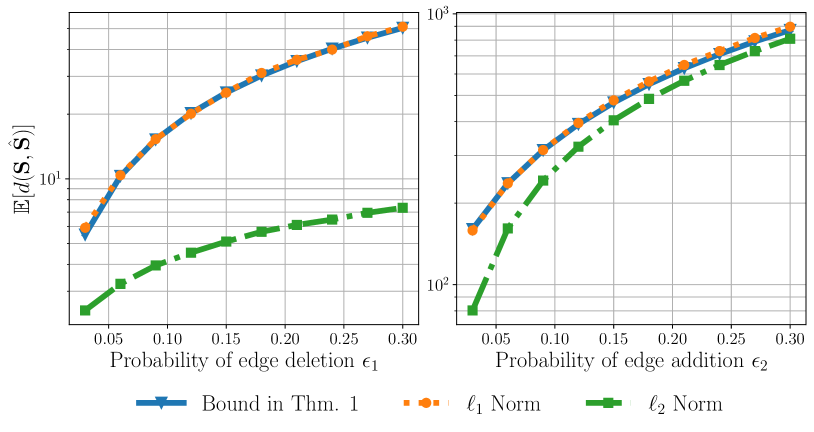
Figure 2: Perturbed Cora graph’s theoretical and empirical bounds, featuring the GSO as ${\mathbf{S}}={\mathbf{A}}$. The left side depicts the scenario with a constant $\epsilon_{2}=0$ and varying $\epsilon_{1}\in[3\times 10^{-2},3\times 10^{-1}]$, and the right side represents the case with a steady $\epsilon_{1}=5\times 10^{-1}$ and varying $\epsilon_{2}\in[3\times 10^{-2},3\times 10^{-1}]$. Our theoretical bound is in alignment with the empirical $\ell_{1}$ bound, which signifies our model’s robustness.

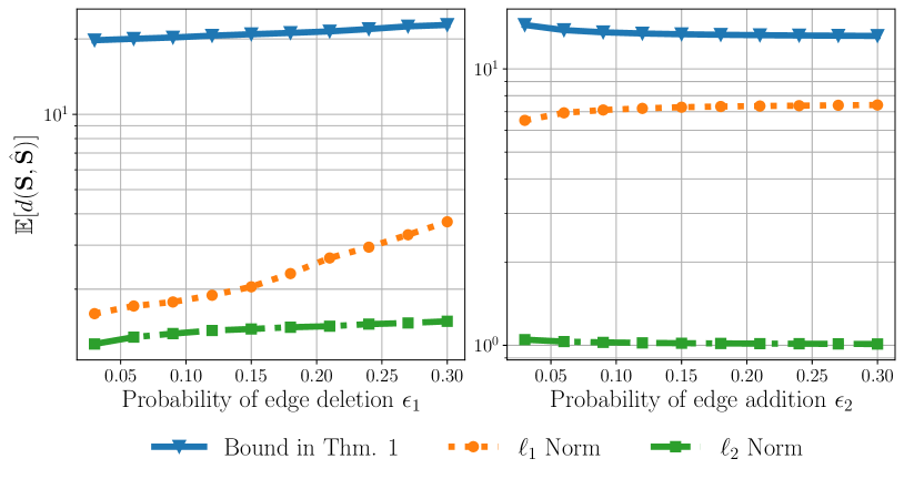
Figure 3: Perturbed Cora graph’s theoretical and empirical bounds, featuring the GSO as ${\mathbf{S}}={\mathbf{A}}_{\textrm{n}}$. The settings for $(\epsilon_{1},\epsilon_{2})$ are identical to the previous figure. It illustrates the differing responses of the bounds to variations in $\epsilon_{1}$ and $\epsilon_{2}$.

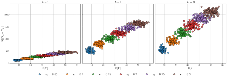
Figure 4: The correlation between observed differences in GIN output and GSO distances for varying edge deletion probabilities, $\epsilon_{1}$. Results for each edge deletion probability are depicted by different colored groups, with 101 Monte Carlo trials used to compute pairs of GSO distances and GIN output differences.

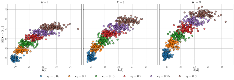
Figure 5: The correlation between observed differences in SGCN output and GSO distances for varying edge deletion probabilities, $\epsilon_{1}$. Results for each edge deletion probability are depicted by different colored groups, with 101 Monte Carlo trials used to compute pairs of GSO distances and SGCN output differences.

We utilize the undirected Cora citation graph [41], which comprises $N=2708$ nodes, and $C=7$ classes. Assuming the undirected nature of the underlying graph, we modify the original Cora graph from a directed to an undirected one. The undirected Cora graph has $|{\mathcal{E}}|=5278$ edges. We ascertain the evolution of our theoretical bounds against an increase in edge deletion probability $\epsilon_{1}$ and edge addition probability $\epsilon_{2}$. These alterations are systematically tracked along with using the $\ell_{1}$ and $\ell_{2}$ norms of the discrepancy between the original and perturbed graphs.

The analysis navigates through $\epsilon_{1}$ and $\epsilon_{2}$ values between $3\times 10^{-2}$ and $3\times 10^{-1}$, augmented in $3\times 10^{-2}$ intervals. Each step involves computing the $\ell_{1}$ and $\ell_{2}$ norms of the difference between the original and perturbed adjacency matrices, with the derived empirical data subsequently juxtaposed against theoretical bounds (Theorem 1 and approximation (24)).

In Fig. 2, we set the GSO as the unnormalized adjacency matrix ${\mathbf{S}}={\mathbf{A}}$. The figure distinguishes between scenarios where $\epsilon_{2}$ is fixed at 0 with varying $\epsilon_{1}$ (left side), and $\epsilon_{1}$ is fixed at $5\times 10^{-1}$ with varying $\epsilon_{2}$ (right side). For each bound, 101 MC iterations are performed. The resulting perturbed adjacency matrices and their associated $\ell_{1}$ and $\ell_{2}$ norms demonstrate that our proposed theoretical bound closely aligns with the empirical $\ell_{1}$ bound. Furthermore, we account for the Cora graph’s sparsity, resulting in more edge deletions than additions when edge deletion and addition probabilities are equal. Consequently, an increased $\epsilon_{2}$ generates denser perturbed graphs, which, in turn, bring the theoretical bound and empirical $\ell_{1}$ norm closer to the $\ell_{2}$ bound. This behavior suggests that our bound’s precision improves as the graphs transition from sparse to dense structures.

In Fig. 3, we set the GSO as the normalized adjacency matrix ${\mathbf{S}}={\mathbf{A}}_{\textrm{n}}$. Similar to the previous figure, we consider two scenarios: the left case sets $\epsilon_{2}$ to 0 and varies $\epsilon_{1}$, while the right case fixes $\epsilon_{1}$ at $5\times 10^{-1}$ and adjusts $\epsilon_{2}$. For each case, we execute 101 MC iterations. The analysis of the left case reveals that all three bounds tend to increase together, confirming the validity of Theorem 3, which predicts an increase in GCN output difference with growing error. However, the tightness of the bound is less satisfactory in the normalized case. On the contrary, the right-hand case illustrates a stable empirical $\ell_{2}$ norm with an increasing number of edges, while the $\ell_{1}$ norm and our bound present slight increases and decreases, respectively. These observations can be attributed to several factors: the normalization operation maintains the adjacency matrix operator norm around 1; an increase in row elements naturally escalates the corresponding $\ell_{1}$ norm; and increases in the elements in the denominator in Lemma 1 lead to a general decrease in the bound.

VI-B Specified GCN sensitivity test

The theoretical analysis outlined in Theorem 3 is further examined through experiments performed on GIN and SGCN detailed in Sections V-C1 and V-C2, respectively. These experiments are conducted on the undirected Cora citation dataset used previously. Our goal is to assess the sensitivity of GIN and SGCN to perturbed GSOs by utilizing an evasion attack. After model training and parameter fixation, we introduce GSO perturbations during the testing phase and evaluate the outcomes. For GIN, each layer is set to have $16$ hidden features, with $1,2,3$-layer GINs only differing in the number of cascaded graph filters with MLPs.

We probe the correlation between empirical differences in GCN output and GSO distances in Fig. 4 and Fig. 5. Specifically, the edge deletion probability, $\epsilon_{1}$, is set at intervals of $5\times 10^{-2}$, ranging from $5\times 10^{-2}$ to $3\times 10^{-1}$, while the edge addition probability, $\epsilon_{2}$, is fixed at $0$. Each colored group in the results corresponds to one edge deletion probability, with 101 MC trials executed within each group to compute pairs of GSO distances and GCN output differences. The y-axis is held constant across all subfigures to visualize differences across varying layers and GSO orders.

The output differences exhibited in the two figures operate within distinct scales. Those corresponding to the normalized GSO (in the case of SGCN) exhibit a relatively gradual variation with increasing perturbation probability, in contrast to those linked with the unnormalized GSO (in the case of GIN), which display a more accelerated variation. This can be attributed to the contributions of the estimated GSO spectral norm $\lambda$, the maximum GSO order $K$, and the set of GCN weights $\{{\mathbf{H}}_{\ell k}\}$.

VII Conclusion and Discussion

The paper introduces an analytical framework to investigate the sensitivity of GCNs under specific graph errors. We have also developed two distinct analytical error bounds for different GSOs in a probabilistic error scenario. Furthermore, explicit error bounds were derived for the sensitivity analysis of graph convolutional filters and GCNs, with a special focus on GIN and SGCN. We validated the theoretical results by numerical experiments, providing insights into the impact of graph structure perturbations on GCN performance.

In this work, our primary focus is on edge perturbations in graphs, while potential modifications to the graph signal and node injections are not considered. Any alterations to the graph signal could be subsumed within the spectral norm when performing sensitivity analysis. However, node injection presents a challenge that cannot be addressed using the current definition of graph distance. This is due to the discrepancy in sizes between the unperturbed and perturbed graphs as the number of nodes increases. A potential solution to this issue could involve redefining the GSO distance using a different metric. In this context, Optimal Transport (OT) and its variants emerge as viable candidates for this task [42, 43, 44]. These methods allow for the augmentation of the smaller graph, facilitating the establishment of a meaningful graph distance metric [45]. Consequently, future research could explore an encompassing approach that considers all of the aforementioned types of graph perturbations. Such an investigation has the potential to yield more comprehensive insights into the resilience of GCNs under perturbations.

Graph regularization methods are commonly used to achieve robust graph learning and estimation [46]. Research on adversarial training of GCNs typically uses specifically designed loss functions to strengthen GCNs against structural and feature perturbations, thus improving their performance resilience against certain graph disturbances [47, 48, 49, 50, 51]. In graph learning, several techniques have been developed to regulate graphs and signals based on specific graph signal assumptions to perform graph estimation [16, 17, 52, 53]. With the inclusion of effective graph regularization, our sensitivity analysis offers insight that can contribute to the development of a uniform metric, paving the way for a more transferable and robust GCN.

Appendix A Upper Bound of $\|{\mathbf{E}}_{u}\|_{1}$

Proof of Lemma 1.

We start with the first term in (21), which is bounded by $\tau_{u}\leq d_{v}$

$$\sum_{v\in{\mathcal{D}}_{u}}\dfrac{1}{\sqrt{d_{u}d_{v}}}\leq\sum_{v\in{\mathcal{D}}_{u}}\dfrac{1}{\sqrt{d_{u}\tau_{u}}}=\dfrac{\delta_{u}^{-}}{\sqrt{d_{u}\tau_{u}}}.$$ (31)

The second and third terms in (21) can be bounded using triangle inequality as follows

$$\sum_{v\in{\mathcal{A}}_{u}}\dfrac{1}{\sqrt{{\hat{d}}_{u}{\hat{d}}_{v}}}+\sum_{v\in{\mathcal{R}}_{u}}\left|\dfrac{1}{\sqrt{d_{u}d_{v}}}-\dfrac{1}{\sqrt{{\hat{d}}_{u}{\hat{d}}_{v}}}\right|$$

$$\leq\sum_{v\in{\mathcal{A}}_{u}}\dfrac{1}{\sqrt{{\hat{d}}_{u}{\hat{d}}_{v}}}+\sum_{v\in{\mathcal{R}}_{u}}\left(\dfrac{1}{\sqrt{d_{u}d_{v}}}+\dfrac{1}{\sqrt{{\hat{d}}_{u}{\hat{d}}_{v}}}\right)$$

$$=\sum_{v\in{\mathcal{R}}_{u}}\dfrac{1}{\sqrt{d_{u}d_{v}}}+\sum_{v\in{\mathcal{A}}_{u}\cap{\mathcal{R}}_{u}}\dfrac{1}{\sqrt{{\hat{d}}_{u}{\hat{d}}_{v}}}$$ (32)

For the first term in (A), we have

$$\sum_{v\in{\mathcal{R}}_{u}}\dfrac{1}{\sqrt{d_{u}d_{v}}}\leq\sum_{v\in{\mathcal{R}}_{u}}\dfrac{1}{\sqrt{d_{u}\tau_{u}}}\leq\dfrac{d_{u}-\delta_{u}^{-}}{\sqrt{d_{u}\tau_{u}}}.$$ (33)

For the second term in (A), we have

$$\sum_{v\in{\mathcal{A}}_{u}\cap{\mathcal{R}}_{u}}\dfrac{1}{\sqrt{{\hat{d}}_{u}{\hat{d}}_{v}}}$$

$$=\sum_{v\in{\mathcal{A}}_{u}\cap{\mathcal{R}}_{u}}\dfrac{1}{\sqrt{(d_{u}+\delta_{u}^{+}-\delta_{u}^{-})(d_{v}+\delta_{v}^{+}-\delta_{v}^{-})}}$$

$$\leq\sum_{v\in{\mathcal{N}}_{u}}\dfrac{1}{\sqrt{(d_{u}+\delta_{u}^{+}-\delta_{u}^{-})(d_{v}+\delta_{v}^{+}-\delta_{v}^{-})}}.$$ (34)

Thus, we have a new bound, which is more suited to our error model, that is

$$\begin{split}&\|{\mathbf{E}}_{u}\|_{1}\leq\dfrac{\delta_{u}^{-}}{\sqrt{d_{u}\tau_{u}}}+\dfrac{d_{u}-\delta_{u}^{-}}{\sqrt{d_{u}\tau_{u}}}\\ &+\sum_{v\in{\mathcal{N}}_{u}}\dfrac{1}{\sqrt{(d_{u}+\delta_{u}^{+}-\delta_{u}^{-})(d_{v}+\delta_{v}^{+}-\delta_{v}^{-})}}\\ &=\sqrt{d_{u}/\tau_{u}}+\sum_{v\in{\mathcal{N}}_{u}}\dfrac{1}{\sqrt{(d_{u}+\delta_{u}^{+}-\delta_{u}^{-})(d_{v}+\delta_{v}^{+}-\delta_{v}^{-})}}.\end{split}$$ (35)

We will adapt the general bound (35) to the probabilistic error model presented in (9). The RHS of (35) can be written as a function

$$f_{u}(\delta_{u}^{-},\delta_{u}^{+},\delta_{v}^{-},\delta_{v}^{+})$$

$$=\sqrt{d_{u}/\tau_{u}}+\sum_{v\in{\mathcal{N}}_{u}}\frac{1}{\sqrt{(d_{u}+\delta_{u}^{+}-\delta_{u}^{-})(d_{v}+\delta_{v}^{+}-\delta_{v}^{-})}},$$ (36)

where $\delta_{u}^{-}\sim\textrm{Bin}(d_{u},\epsilon_{1})$, $\delta_{u}^{+}\sim\textrm{Bin}(d_{u}^{*},\epsilon_{2})$, $\delta_{v}^{-}\sim\textrm{Bin}(d_{v},\epsilon_{1})$, $\delta_{v}^{+}\sim\textrm{Bin}(d_{v}^{*},\epsilon_{2})$, $d_{u}^{*}=N-d_{u}-1$ and $d_{v}^{*}=N-d_{v}-1$. This completes the proof. ∎

Appendix B Graph filter sensitivity

Proof of Theorem 2.

First, we recall the following result.

Lemma 2.

(Lemma 3, [54]) Suppose that $\hat{{\mathbf{S}}},{\mathbf{S}},{\mathbf{E}}\in\mathbb{R}^{N\times N}$ are Hermitian matrices satisfying $\hat{{\mathbf{S}}}={\mathbf{S}}+{\mathbf{E}}$, and $\lambda=\max\{\|{\hat{\mathbf{S}}}\|,\|{\mathbf{S}}\|\}$. Then for every $k\geq 0$

$$\|\hat{{\mathbf{S}}}^{k}-{\mathbf{S}}^{k}\|=\|({\mathbf{S}}+{\mathbf{E}})^{k}-{\mathbf{S}}^{k}\|\leq k\lambda^{k-1}\|{\mathbf{E}}\|.$$ (37)

Expand the filter representation in $\|{\mathbf{H}}({\hat{\mathbf{S}}})-{\mathbf{H}}({\mathbf{S}})\|$, as

$$\begin{split}&\|{\mathbf{H}}({\hat{\mathbf{S}}})-{\mathbf{H}}({\mathbf{S}})\|=\left\|\sum_{k=1}^{K}\left({\hat{\mathbf{S}}}^{k}{\mathbf{H}}_{k}-{\mathbf{S}}^{k}{\mathbf{H}}_{k}\right)\right\|.\end{split}$$ (38)

By Lemma 2 and repeatably using triangle inequality, (38) is bounded by

$$\begin{split}&\left\|\sum_{k=1}^{K}\left({\hat{\mathbf{S}}}^{k}{\mathbf{H}}_{k}-{\mathbf{S}}^{k}{\mathbf{H}}_{k}\right)\right\|\leq\sum_{k=1}^{K}\left\|{\hat{\mathbf{S}}}^{k}{\mathbf{H}}_{k}-{\mathbf{S}}^{k}{\mathbf{H}}_{k}\right\|\\ &\leq\sum_{k=1}^{K}\left\|{\mathbf{H}}_{k}\right\|\|{\hat{\mathbf{S}}}^{k}-{\mathbf{S}}^{k}\|\leq\sum_{k=1}^{K}k\lambda^{k-1}\|{\mathbf{H}}_{k}\|\|{\mathbf{E}}\|.\end{split}$$ (39)

This completes the proof. ∎

Appendix C GCN Sensitivity

Proof of Theorem 3.

First Layer. At the first layer $\ell=1$, the graph convolution is performed as follows

$${\mathbf{Y}}_{1}=\sum_{k=1}^{K}{\mathbf{S}}^{k}{\mathbf{X}}_{0}{\mathbf{H}}_{1k},\quad{\mathbf{X}}_{1}=\sigma_{1}({\mathbf{Y}}_{1}).$$

For a perturbed GSO ${\hat{\mathbf{S}}}$, the difference between the perturbed and clean graph convolutions is

$${\hat{\mathbf{Y}}}_{1}-{\mathbf{Y}}_{1}=\sum_{k=1}^{K}({\hat{\mathbf{S}}}^{k}-{\mathbf{S}}^{k}){\mathbf{X}}_{0}{\mathbf{H}}_{1k}.$$ (40)

Using Lemma 2, we can bound (40) as follows

$$\left\|{\hat{\mathbf{Y}}}_{1}-{\mathbf{Y}}_{1}\right\|\leq\sum_{k=1}^{K}k\lambda^{k-1}\|{\mathbf{X}}_{0}\|\|{\mathbf{H}}_{1k}\|\|{\mathbf{E}}\|.$$ (41)

The correlation between $\lambda$ and $\|{\mathbf{E}}\|$ has two cases:

1. If $\lambda=\|{\mathbf{S}}\|$,

   $$\mathbb{E}[\lambda^{k-1}\|\mathbf{E}\|]=\mathbb{E}[\lambda^{k-1}]\mathbb{E}[\|\mathbf{E}\|],$$ (42)

2. If $\lambda=\|{\hat{\mathbf{S}}}\|$,

   $$\mathbb{E}[\lambda^{k-1}\|\mathbf{E}\|]=\mathbb{E}[\lambda^{k-1}]\mathbb{E}[\|\mathbf{E}\|]+\textrm{Cov}[\|\mathbf{E}\|,\lambda^{k-1}].$$ (43)

The following proof is based on the second case (43) because the covariance term can be set to zero to include the first case. By taking the expectation of (41), we obtain

$${\mathbb{E}}\left[\left\|{\hat{\mathbf{Y}}}_{1}-{\mathbf{Y}}_{1}\right\|\right]\leq{\mathbb{E}}\left[\sum_{k=1}^{K}k\lambda^{k-1}\|{\mathbf{X}}_{0}\|\|{\mathbf{H}}_{1k}\|\|{\mathbf{E}}\|\right]$$

$$=\sum_{k=1}^{K}k\|{\mathbf{X}}_{0}\|\|{\mathbf{H}}_{1k}\|{\mathbb{E}}\left[\lambda^{k-1}\|{\mathbf{E}}\|\right]$$

$$=\sum_{k=1}^{K}k\|{\mathbf{X}}_{0}\|\|{\mathbf{H}}_{1k}\|\left({\mathbb{E}}[\lambda^{k-1}]{\mathbb{E}}\left[\|{\mathbf{E}}\|\right]+\textrm{Cov}[\|{\mathbf{E}}\|,\lambda^{k-1}]\right).$$ (44)

In (44), let

$$\lambda_{k}={\mathbb{E}}[\lambda^{k-1}]\ \text{for}\ k=1,\ldots,K.$$

Similarly, for $\{\textrm{Cov}[\|{\mathbf{E}}\|,\lambda^{k-1}]\}_{k=1}^{K}$ in (44), we have their upper bounds as

$$\textrm{Cov}[\|{\mathbf{E}}\|,\lambda^{k-1}]\leq\sqrt{\mathrm{Var}[\|{\mathbf{E}}\|]\mathrm{Var}[\lambda^{k-1}]}.$$ (45)

In (45), let

$$\zeta_{k}=\sqrt{\mathrm{Var}[\|{\mathbf{E}}\|]\mathrm{Var}[\lambda^{k-1}]}\ \text{for}\ k=1,\ldots,K.$$

Then, (44) can be written as

$${\mathbb{E}}\left[\left\|{\hat{\mathbf{Y}}}_{1}-{\mathbf{Y}}_{1}\right\|\right]\leq\sum_{k=1}^{K}k\|{\mathbf{X}}_{0}\|\|{\mathbf{H}}_{1k}\|\left(\lambda_{k}{\mathbb{E}}\left[\|{\mathbf{E}}\|\right]+\zeta_{k}\right).$$ (46)

For simplicity, let $B_{1}=\sum_{k=1}^{K}k\lambda_{k}\|{\mathbf{X}}_{0}\|\|{\mathbf{H}}_{1k}\|$, and $D_{1}=\sum_{k=1}^{K}k\zeta_{k}\|{\mathbf{X}}_{0}\|\|{\mathbf{H}}_{1k}\|$. Thus, (46) illustrates that the expectation of the graph filter distance at the first layer is bounded by a polynomial of ${\mathbb{E}}\left[\|{\mathbf{E}}\|\right]$ as

$${\mathbb{E}}\left[\left\|{\hat{\mathbf{Y}}}_{1}-{\mathbf{Y}}_{1}\right\|\right]\leq B_{1}{\mathbb{E}}[\|{\mathbf{E}}\|]+D_{1}.$$

Consider the nonlinearity function $\sigma_{1}(\cdot)$ at the first layer, which satisfies the Lipschitz condition

$$\|\sigma_{1}({\hat{\mathbf{Y}}})-\sigma_{1}({\mathbf{Y}})\|\leq C_{\sigma_{1}}\|{\hat{\mathbf{Y}}}-{\mathbf{Y}}\|.$$

Applying this Lipschitz condition to (41), we have

$${\mathbb{E}}\left[\|{\hat{\mathbf{X}}}_{1}-{\mathbf{X}}_{1}\|\right]={\mathbb{E}}\left[\left\|\sigma_{1}({\hat{\mathbf{Y}}})-\sigma_{1}({\mathbf{Y}})\right\|\right]$$

$$\leq C_{\sigma_{1}}{\mathbb{E}}\left[\left\|{\hat{\mathbf{Y}}}-{\mathbf{Y}}\right\|\right]\leq C_{\sigma_{1}}B_{1}{\mathbb{E}}\left[\|{\mathbf{E}}\|\right]+C_{\sigma_{1}}D_{1}.$$ (47)

Second Layer. At the second layer $\ell=2$, the graph convolution is performed as

$${\mathbf{Y}}_{2}=\sum_{k=1}^{K}{\mathbf{S}}^{k}{\mathbf{X}}_{1}{\mathbf{H}}_{2k},\quad{\mathbf{X}}_{2}=\sigma({\mathbf{Y}}_{2}).$$

The difference between the perturbed and clean graph convolutions is given by

$${\hat{\mathbf{Y}}}_{2}-{\mathbf{Y}}_{2}=\sum_{k=1}^{K}{\hat{\mathbf{S}}}^{k}{\hat{\mathbf{X}}}_{1}{\mathbf{H}}_{2k}-\sum_{k=1}^{K}{\mathbf{S}}^{k}{\mathbf{X}}_{1}{\mathbf{H}}_{2k}$$

$$=\sum_{k=1}^{K}({\hat{\mathbf{S}}}^{k}{\hat{\mathbf{X}}}_{1}-{\hat{\mathbf{S}}}^{k}{\mathbf{X}}_{1}+{\hat{\mathbf{S}}}^{k}{\mathbf{X}}_{1}-{\mathbf{S}}^{k}{\mathbf{X}}_{1}){\mathbf{H}}_{2k}$$

$$=\sum_{k=1}^{K}\left({\hat{\mathbf{S}}}^{k}({\hat{\mathbf{X}}}_{1}-{\mathbf{X}}_{1})+({\hat{\mathbf{S}}}^{k}-{\mathbf{S}}^{k}){\mathbf{X}}_{1}\right){\mathbf{H}}_{2k}.$$ (48)

Taking the expectation of (C) and using (43), Lemma 2 as well as the submultiplicativity of the spectral norm, we have

$${\mathbb{E}}\left[\left\|{\hat{\mathbf{Y}}}_{2}-{\mathbf{Y}}_{2}\right\|\right]$$

$$\leq{\mathbb{E}}\left[\left\|\sum_{k=1}^{K}\left({\hat{\mathbf{S}}}^{k}({\hat{\mathbf{X}}}_{1}-{\mathbf{X}}_{1})+({\hat{\mathbf{S}}}^{k}-{\mathbf{S}}^{k}){\mathbf{X}}_{1}\right){\mathbf{H}}_{2k}\right\|\right]$$

$$\leq\sum_{k=1}^{K}\|{\mathbf{H}}_{2k}\|{\mathbb{E}}\left[\left\|{\hat{\mathbf{S}}}^{k}({\hat{\mathbf{X}}}_{1}-{\mathbf{X}}_{1})\right\|+\left\|({\hat{\mathbf{S}}}^{k}-{\mathbf{S}}^{k}){\mathbf{X}}_{1}\right\|\right]$$

$$\leq\sum_{k=1}^{K}\|{\mathbf{H}}_{2k}\|\Big{(}{\mathbb{E}}[\lambda^{k}]{\mathbb{E}}\left[\|{\hat{\mathbf{X}}}_{1}-{\mathbf{X}}_{1}\|\right]+\text{Cov}\left[\|{\hat{\mathbf{X}}}_{1}-{\mathbf{X}}_{1}\|,\lambda^{k}\right]$$

$$+k\|{\mathbf{X}}_{1}\|\left({\mathbb{E}}[\lambda^{k-1}]{\mathbb{E}}\left[\|{\mathbf{E}}\|\right]+\textrm{Cov}[\|{\mathbf{E}}\|,\lambda^{k-1}]\right)\Bigr{)}.$$ (49)

For $\{\text{Cov}[\|{\hat{\mathbf{X}}}_{1}-{\mathbf{X}}_{1}\|,\lambda^{k}]\}_{k=1}^{K}$ in (49), we can bound it with constants using the similar way as in (45)

$$\text{Cov}[\|{\hat{\mathbf{X}}}_{1}-{\mathbf{X}}_{1}\|,\lambda^{k}]\leq\sqrt{\mathrm{Var}[\|{\hat{\mathbf{X}}}_{1}-{\mathbf{X}}_{1}\|]\mathrm{Var}[\lambda^{k}]}.$$ (50)

We use constants $\{\mu_{k,\ell-1}\}_{k=1,\ell=2}^{K,L}$ to denote the upper bounds $\mu_{k,1}=\sqrt{\mathrm{Var}[\|{\hat{\mathbf{X}}}_{1}-{\mathbf{X}}_{1}\|]\mathrm{Var}[\lambda^{k}]}$. By using the result from the first layer (47), we can express (49) as a function controlled by ${\mathbb{E}}[\|{\mathbf{E}}\|]$

$${\mathbb{E}}\left[\left\|{\hat{\mathbf{Y}}}_{2}-{\mathbf{Y}}_{2}\right\|\right]\leq\sum_{k=1}^{K}\|{\mathbf{H}}_{2k}\|\Bigl{(}\lambda_{k+1}{\mathbb{E}}\left[\|{\hat{\mathbf{X}}}_{1}-{\mathbf{X}}_{1}\|\right]$$

$$+\mu_{k,1}+k\lambda_{k}\|{\mathbf{X}}_{1}\|{\mathbb{E}}[\|{\mathbf{E}}\|]+k\zeta_{k}\|{\mathbf{X}}_{1}\|\Bigr{)}$$

$$\leq\sum_{k=1}^{K}\|{\mathbf{H}}_{2k}\|\Bigl{(}\left(\lambda_{k+1}C_{\sigma_{1}}B_{1}+k\lambda_{k}\|{\mathbf{X}}_{1}\|\right){\mathbb{E}}[\|{\mathbf{E}}\|]$$

$$+\mu_{k,1}+\lambda_{k}C_{\sigma_{1}}D_{1}+k\zeta_{k}\|{\mathbf{X}}_{1}\|\Bigr{)}$$

$$\leq B_{2}{\mathbb{E}}[\|{\mathbf{E}}\|]+D_{2},$$

where $B_{2}=\sum_{k=1}^{K}\left(\lambda_{k+1}C_{\sigma_{1}}B_{1}+k\lambda_{k}\|{\mathbf{X}}_{1}\|\right)\|{\mathbf{H}}_{2k}\|$ and $D_{2}=\sum_{k=1}^{K}\left(\mu_{k,1}+\lambda_{k}C_{\sigma_{1}}D_{1}+k\zeta_{k}\|{\mathbf{X}}_{1}\|\right)\|{\mathbf{H}}_{2k}\|$. Consider the second layer’s nonlinearity function $\sigma_{2}(\cdot)$, we have

$${\mathbb{E}}\left[\|{\hat{\mathbf{X}}}_{2}-{\mathbf{X}}_{2}\|\right]\leq C_{\sigma_{2}}B_{2}{\mathbb{E}}[\|{\mathbf{E}}\|]+C_{\sigma_{2}}D_{2}.$$

Generalization to Layer $\ell\geq 1$. By induction, we can generalize the result to the output difference at any layer $\ell\geq 1$

$${\mathbb{E}}\left[\left\|{\hat{\mathbf{X}}}_{\ell}-{\mathbf{X}}_{\ell}\right\|\right]\leq C_{\sigma_{\ell}}B_{\ell}{\mathbb{E}}\left[\|{\mathbf{E}}\|\right]+C_{\sigma_{\ell}}D_{\ell},$$ (51)

where

$$B_{\ell} =\sum_{k=1}^{K}\left(\lambda_{k+1}C_{\sigma_{\ell-1}}B_{\ell-1}+k\lambda_{k}\|{\mathbf{X}}_{\ell-1}\|\right)\|{\mathbf{H}}_{\ell k}\|,$$

$$D_{\ell} =\sum_{k=1}^{K}\left(\mu_{k,\ell-1}+\lambda_{k}C_{\sigma_{\ell-1}}D_{\ell-1}+k\zeta_{k}\|{\mathbf{X}}_{\ell-1}\|\right)\|{\mathbf{H}}_{\ell k}\|.$$

Finally, applying the inequality ${\mathbb{E}}[\|{\mathbf{E}}\|]\leq{\mathbb{E}}[\|{\mathbf{E}}\|_{1}]$ in (20) completes the proof. ∎

Appendix D GIN Perceptron Sensitivity

Proof.

Given the intermediate output of graph filter with original and perturbed GSOs as

$${\mathbf{Y}}_{\ell}=\boldsymbol{\Theta}_{\ell}\bigl{(}{\mathbf{S}}{\mathbf{X}}_{\ell-1}{\mathbf{H}}_{\ell 1}\bigr{)},{\hat{\mathbf{Y}}}_{\ell}=\boldsymbol{\Theta}_{\ell}\bigl{(}{\hat{\mathbf{S}}}{\mathbf{X}}_{\ell-1}{\mathbf{H}}_{\ell 1}\bigr{)}$$

then, the transformations for original and perturbed GSOs inside this MLP are ${\mathbf{X}}^{\prime}_{\ell}=\sigma^{\prime}_{\ell}\bigl{(}({\mathbf{S}}{\mathbf{X}}_{\ell-1}{\mathbf{H}}_{\ell 1}){\mathbf{W}}^{\prime}_{\ell}+{\mathbf{B}}^{\prime}_{\ell}\bigr{)},{\mathbf{Y}}_{\ell}={\mathbf{X}}^{\prime}_{\ell}{\mathbf{W}}^{\prime\prime}_{\ell}+{\mathbf{B}}^{\prime\prime}_{\ell},{\mathbf{X}}_{\ell}=\sigma_{\ell}({\mathbf{Y}}_{\ell}),$ and ${\hat{\mathbf{X}}}^{\prime}_{\ell}=\sigma^{\prime}_{\ell}\bigl{(}({\mathbf{S}}{\hat{\mathbf{X}}}_{\ell-1}{\mathbf{H}}_{\ell 1}){\mathbf{W}}^{\prime}_{\ell}+{\mathbf{B}}^{\prime}_{\ell}\bigr{)},{\hat{\mathbf{Y}}}_{\ell}={\hat{\mathbf{X}}}^{\prime}_{\ell}{\mathbf{W}}^{\prime\prime}_{\ell}+{\mathbf{B}}^{\prime\prime}_{\ell},{\hat{\mathbf{X}}}_{\ell}=\sigma_{\ell}({\hat{\mathbf{Y}}}_{\ell}),$ respectively. Using triangular inequality multiple times and ${\mathbf{E}}={\hat{\mathbf{S}}}-{\mathbf{S}}$, the expectation of outputs’ difference is as

$${\mathbb{E}}\left[\|{\hat{\mathbf{X}}}_{\ell}-{\mathbf{X}}_{\ell}\|\right]\leq C_{\sigma_{\ell}}\|{\mathbf{W}}^{\prime\prime}_{\ell}\|{\mathbb{E}}\left[\|{\hat{\mathbf{X}}}^{\prime}_{\ell}-{\mathbf{X}}^{\prime}_{\ell}\|\right],$$

where

$${\mathbb{E}}\left[\|{\hat{\mathbf{X}}}^{\prime}_{\ell}-{\mathbf{X}}^{\prime}_{\ell}\|\right]\leq C_{\sigma^{\prime}_{\ell}}\|{\mathbf{X}}_{\ell-1}\|\|{\mathbf{H}}_{\ell 1}\|\|{\mathbf{W}}^{\prime}_{\ell}\|{\mathbb{E}}\left[\|{\hat{\mathbf{S}}}-{\mathbf{S}}\|\right].$$

Thus, we conclude that

$$\begin{split}&{\mathbb{E}}\left[\|{\hat{\mathbf{X}}}_{\ell}-{\mathbf{X}}_{\ell}\|\right]\leq\xi_{\ell}{\mathbb{E}}[\|{\mathbf{E}}\|],\\ &\xi_{\ell}=C_{\sigma_{\ell}}C_{\sigma^{\prime}_{\ell}}\|{\mathbf{X}}_{\ell-1}\|\|{\mathbf{H}}_{\ell 1}\|\|{\mathbf{W}}^{\prime}_{\ell}\|\|{\mathbf{W}}^{\prime\prime}_{\ell}\|.\end{split}$$ (52)

This completes the proof. ∎

References

- [1] M. M. Bronstein, J. Bruna, Y. LeCun, A. Szlam, and P. Vandergheynst, “Geometric deep learning: Going beyond Euclidean data,” IEEE Signal Process. Mag., vol. 34, no. 4, pp. 18–42, July. 2017.
- [2] X. Dong, D. Thanou, L. Toni, M. Bronstein, and P. Frossard, “Graph signal processing for machine learning: A review and new perspectives,” IEEE Signal Process. Mag., vol. 37, no. 6, pp. 117–127, Oct. 2020.
- [3] Z. Wu, S. Pan, F. Chen, G. Long, C. Zhang, and P. S. Yu, “A comprehensive survey on graph neural networks,” IEEE Trans. Neural Netw. Learning Syst., vol. 32, no. 1, pp. 4–24, March. 2021.
- [4] E. Isufi, F. Gama, D. I. Shuman, and S. Segarra, “Graph filters for signal processing and machine learning on graphs,” arXiv:2211.08854, [eess.SP], 2022.
- [5] L. Ruiz, F. Gama, and A. Ribeiro, “Graph neural networks: Architectures, stability, and transferability,” Proc. of the IEEE, vol. 109, no. 5, pp. 660–682, Feb. 2021.
- [6] T. N. Kipf and M. Welling, “Semi-supervised classification with graph convolutional networks,” in Proc. 5th Int. Conf. Learn. Representations, Toulon, France, Apr. 24-26, 2017, pp. 1–14.
- [7] Q. Li, X.-M. Wu, H. Liu, X. Zhang, and Z. Guan, “Label efficient semi-supervised learning via graph filtering,” in Proc. 32nd Conf. Comput. Vision and Pattern Recognition, Long Beach, CA, USA, June 16-20, 2019, pp. 9574–9583.
- [8] F. Wu, T. Zhang, A. H. d. Souza, Jr, C. Fifty, T. Yu, and K. Q. Weinberger, “Simplifying graph convolutional networks,” in Proc. 36th Int. Conf. Mach. Learning, Long Beach, California, USA, June 9-15, 2019, pp. 6861–6871.
- [9] R. Levie, F. Monti, X. Bresson, and M. M. Bronstein, “Cayleynets: Graph convolutional neural networks with complex rational spectral filters,” IEEE Trans. Signal Process., vol. 67, no. 1, pp. 97–109, Nov. 2019.
- [10] P. Velickovic, G. Cucurull, A. Casanova, A. Romero, P. Liò, and Y. Bengio, “Graph attention networks,” in Proc. 6th Int. Conf. Learn. Representations, Vancouver, BC, Canada, Apr. 30 - May. 3, 2018.
- [11] E. Isufi, F. Gama, and A. Ribeiro, “EdgeNets: Edge varying graph neural networks,” IEEE Trans. Pattern Anal. Mach. Intell., vol. 44, no. 11, pp. 7457–7473, Sept. 2022.
- [12] M. Coutino, E. Isufi, and G. Leus, “Advances in distributed graph filtering,” IEEE Trans. Signal Process., vol. 67, no. 9, pp. 2320–2333, March. 2019.
- [13] A. Sandryhaila and J. M. F. Moura, “Discrete signal processing on graphs,” IEEE Trans. Signal Process., vol. 61, no. 7, pp. 1644–1656, Apr. 2013.
- [14] M. Defferrard, X. Bresson, and P. Vandergheynst, “Convolutional neural networks on graphs with fast localized spectral filtering,” in Proc. 30th Conf. Neural Inform. Process. Syst., Barcelona, Spain, Dec. 5-10, 2016, pp. 3844–3858.
- [15] K. Xu, W. Hu, J. Leskovec, and S. Jegelka, “How powerful are graph neural networks?” in Proc. 7th Int. Conf. Learn. Representations, New Orleans, LA, USA, May 6-9, 2019, pp. 1–17.
- [16] X. Dong, D. Thanou, P. Frossard, and P. Vandergheynst, “Learning laplacian matrix in smooth graph signal representations,” IEEE Trans. Signal Process., vol. 64, no. 23, pp. 6160–6173, Dec. 2016.
- [17] S. Segarra, A. G. Marques, G. Mateos, and A. Ribeiro, “Network topology inference from spectral templates,” IEEE Trans. Signal Inf. Process. Netw., vol. 3, no. 3, pp. 467–483, July. 2017.
- [18] A. Buciulea, S. Rey, and A. G. Marques, “Learning graphs from smooth and graph-stationary signals with hidden variables,” IEEE Trans. Signal Inf. Process. Netw., vol. 8, pp. 273–287, March. 2022.
- [19] J. Miettinen, S. A. Vorobyov, and E. Ollila, “Modelling and studying the effect of graph errors in graph signal processing,” Signal Process., vol. 189, 108256, pp. 1–8, Dec. 2021.
- [20] A. Ghosh and S. Boyd, “Growing well-connected graphs,” in Proc. 45th IEEE Conf. Decision, Control, San Diego, CA, USA, Dec. 13-15, 2006, pp. 6605–6611.
- [21] A. Sydney, C. Scoglio, and D. Gruenbacher, “Optimizing algebraic connectivity by edge rewiring,” Appl. Math. Comput., vol. 219, no. 10, pp. 5465–5479, Jan. 2013.
- [22] K. Xu, H. Chen, S. Liu, P.-Y. Chen, T.-W. Weng, M. Hong, and X. Lin, “Topology attack and defense for graph neural networks: An optimization perspective,” in Proc. 28th Int. Joint Conf. Artif. Intell., Macao, China, Aug. 10-16, 2019, pp. 3961–3967.
- [23] E. Ceci and S. Barbarossa, “Graph signal processing in the presence of topology uncertainties,” IEEE Trans. Signal Process., vol. 68, pp. 1558–1573, Feb. 2020.
- [24] Z. Gao, E. Isufi, and A. Ribeiro, “Stability of graph convolutional neural networks to stochastic perturbations,” Signal Process., vol. 188, 108216, pp. 1–15, Nov. 2021.
- [25] S. Verma and Z.-L. Zhang, “Stability and generalization of graph convolutional neural networks,” in Proc. 25th ACM SIGKDD Int. Conf. Knowl. Discov. & Data Mining, Anchorage, AK, USA, Aug. 4-8, 2019, pp. 1539–1548.
- [26] F. Gama, J. Bruna, and A. Ribeiro, “Stability properties of graph neural networks,” IEEE Trans. Signal Process., vol. 68, pp. 5680–5695, Sep. 2020.
- [27] N. Keriven, A. Bietti, and S. Vaiter, “Convergence and stability of graph convolutional networks on large random graphs,” in Proc. 33th Conf. Neural Inform. Process. Syst., H. Larochelle, M. Ranzato, R. Hadsell, M. Balcan, and H. Lin, Eds., vol. 33, Virtual, Dec. 7-12, 2020, pp. 21 512–21 523.
- [28] D. Zügner and S. Günnemann, “Certifiable robustness of graph convolutional networks under structure perturbations,” in Proc. 26th ACM SIGKDD Int. Conf. Knowl. Discov. & Data Mining, Virtual, July 6-10, 2020, p. 1656–1665.
- [29] H. Kenlay, D. Thano, and X. Dong, “On the stability of graph convolutional neural networks under edge rewiring,” in Proc. 46th IEEE Int. Conf. Acoustic, Speech and Signal Process., Toronto, Canada, June 6-11, 2021, pp. 8513–8517.
- [30] H. Dai, H. Li, T. Tian, X. Huang, L. Wang, J. Zhu, and L. Song, “Adversarial attack on graph structured data,” in Proc. 35th Int. Conf. Mach. Learning, vol. 80, Stockholm, Sweden, July 10-15, 2018, pp. 1115–1124.
- [31] H. Wu, C. Wang, Y. Tyshetskiy, A. Docherty, K. Lu, and L. Zhu, “Adversarial examples for graph data: Deep insights into attack and defense,” in Proc. 28th Int. Joint Conf. Artif. Intell., Macao, China, Aug. 10-16, 2019, pp. 4816–4823.
- [32] X. Wang, X. Liu, and C.-J. Hsieh, “Graphdefense: Towards robust graph convolutional networks,” arXiv:1911.04429, [cs.LG], 2019.
- [33] L. Lin, E. Blaser, and H. Wang, “Graph structural attack by perturbing spectral distance,” in Proc. 28th ACM SIGKDD Int. Conf. Knowl. Discov. & Data Mining, Washington DC, USA, Aug. 14-18 2022, p. 989–998.
- [34] D. I. Shuman, S. K. Narang, P. Frossard, A. Ortega, and P. Vandergheynst, “The emerging field of signal processing on graphs: Extending high-dimensional data analysis to networks and other irregular domains,” IEEE Signal Process. Mag., vol. 30, no. 3, pp. 83–98, Apr. 2013.
- [35] L. Ruiz, F. Gama, and A. Ribeiro, “Graph neural networks: Architectures, stability, and transferability,” Proc. IEEE, vol. 109, no. 5, pp. 660–682, Feb. 2021.
- [36] H. Kenlay, D. Thanou, and X. Dong, “Interpretable stability bounds for spectral graph filters,” in Proc. 38th Int. Conf. Mach. Learning, vol. 139, Virtual, July 18-24, 2021, pp. 5388–5397.
- [37] M. Penrose, “Random geometric graphs,” Oxford Stud. in Probab., vol. 5, 2003.
- [38] A. Hagberg, P. Swart, and D. S Chult, “Exploring network structure, dynamics, and function using networkx,” Los Alamos National Lab., Los Alamos, NM, USA, Tech. Rep., 2008.
- [39] X. Wang, E. Ollila, and S. A. Vorobyov, “Graph neural network sensitivity under probabilistic error model,” in Proc. 30th Eur. Signal Process. Conf., Belgrade, Serbia, Aug. 29-Sept. 2, 2022, pp. 2146–2150.
- [40] B. Weisfeiler and A. Lehman, “A reduction of a graph to a canonical form and an algebra arising during this reduction,” Nauchno-Technicheskaya Informatsia, vol. 2, no. 9, pp. 12–16, 1968.
- [41] P. Sen, G. Namata, M. Bilgic, L. Getoor, B. Galligher, and T. Eliassi-Rad, “Collective classification in network data,” AI Magazine, vol. 29, no. 3, p. 93, Sep. 2008.
- [42] L. Chizat, G. Peyré, B. Schmitzer, and F.-X. Vialard, “Unbalanced optimal transport: Dynamic and kantorovich formulations,” J. Funct. Anal., vol. 274, no. 11, pp. 3090–3123, June. 2018.
- [43] L. Chapel, M. Z. Alaya, and G. Gasso, “Partial optimal tranport with applications on positive-unlabeled learning,” in Proc. 33th Conf. Neural Inform. Process. Syst., H. Larochelle, M. Ranzato, R. Hadsell, M. Balcan, and H. Lin, Eds., vol. 33, Virtual, Dec. 7-12 2020, pp. 2903–2913.
- [44] H. P. Maretic, M. El Gheche, M. Minder, G. Chierchia, and P. Frossard, “Wasserstein-based graph alignment,” IEEE Trans. Signal Inf. Process. Netw., vol. 8, pp. 353–363, Apr. 2022.
- [45] C.-Y. Chuang and S. Jegelka, “Tree mover’s distance: Bridging graph metrics and stability of graph neural networks,” in Proc. 35th Conf. Neural Inform. Process. Syst., S. Koyejo, S. Mohamed, A. Agarwal, D. Belgrave, K. Cho, and A. Oh, Eds., vol. 35, New Orleans, USA, Nov. 28 - Dec. 9th 2022, pp. 2944–2957.
- [46] L. Sun, Y. Dou, C. Yang, K. Zhang, J. Wang, P. S. Yu, L. He, and B. Li, “Adversarial attack and defense on graph data: A survey,” IEEE Trans. Knowl. Data Eng., pp. 1–20, Sept. 2022.
- [47] H. Jin and X. Zhang, “Latent adversarial training of graph convolution networks,” in Proc. 36th Int. Conf. Mach. Learning Workshop Learn. Reasoning with Graph-structured Representations, Long Beach, California, USA, June 9-15, 2019, pp. 1–7.
- [48] F. Feng, X. He, J. Tang, and T.-S. Chua, “Graph adversarial training: Dynamically regularizing based on graph structure,” IEEE Trans. Knowl. Data Eng., vol. 33, no. 6, pp. 2493–2504, June. 2019.
- [49] Q. Dai, X. Shen, L. Zhang, Q. Li, and D. Wang, “Adversarial training methods for network embedding,” in Proc. 30th The World Wide Web Conf., San Francisco, CA, USA, May 13-17 2019, pp. 329–339.
- [50] J. Ren, Z. Zhang, J. Jin, X. Zhao, S. Wu, Y. Zhou, Y. Shen, T. Che, R. Jin, and D. Dou, “Integrated defense for resilient graph matching,” in Proc. 38th Int. Conf. Mach. Learning, vol. 139, Virtual, July 18-24, 2021, pp. 8982–8997.
- [51] X. Zhao, Z. Zhang, Z. Zhang, L. Wu, J. Jin, Y. Zhou, R. Jin, D. Dou, and D. Yan, “Expressive 1-lipschitz neural networks for robust multiple graph learning against adversarial attacks,” in Proc. 38th Int. Conf. Mach. Learning, vol. 139, July 18-24, 2021, pp. 12 719–12 735.
- [52] H. E. Egilmez, E. Pavez, and A. Ortega, “Graph learning from filtered signals: Graph system and diffusion kernel identification,” IEEE Trans. Signal Inf. Process. Netw., vol. 5, no. 2, pp. 360–374, June. 2018.
- [53] X. Pu, S. L. Chau, X. Dong, and D. Sejdinovic, “Kernel-based graph learning from smooth signals: A functional viewpoint,” IEEE Trans. Signal Inf. Process. Netw., vol. 7, pp. 192–207, Feb. 2021.
- [54] R. Levie, E. Isufi, and G. Kutyniok, “On the transferability of spectral graph filters,” in Proc. 13th Int. Conf. on Sampling Theory and Appl., Bordeaux, France, July 8-12, 2019, pp. 1–5.