Learning to Infer Belief Embedded Communication

Abstract

In multi-agent collaboration problems with communication, an agent’s ability to encode their intention and interpret other agents’ strategies is critical for planning their future actions. This paper introduces a novel algorithm called Intention Embedded Communication (IEC) to mimic an agent’s language learning ability. IEC contains a perception module for decoding other agents’ intentions in response to their past actions. It also includes a language generation module for learning implicit grammar during communication with two or more agents. Such grammar, by construction, should be compact for efficient communication. Both modules undergo conjoint evolution - similar to an infant’s babbling that enables it to learn a language of choice by trial and error. We utilised three multi-agent environments, namely predator/prey, traffic junction and level-based foraging and illustrate that such a co-evolution enables us to learn much quicker (50 %) than state-of-the-art algorithms like MADDPG. Ablation studies further show that disabling the inferring belief module, communication module, and the hidden states reduces the model performance by 38%, 60% and 30%, respectively. Hence, we suggest that modelling other agents’ behaviour accelerates another agent to learn grammar and develop a language to communicate efficiently. We evaluate our method on a set of cooperative scenarios and show its superior performance to other multi-agent baselines. We also demonstrate that it is essential for agents to reason about others’ states and learn this ability by continuous communication.

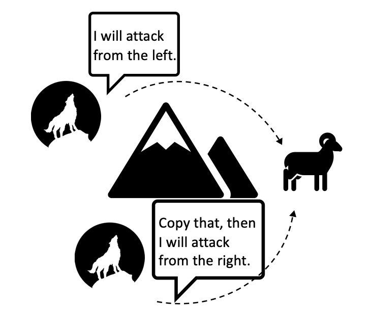
Figure 1: Motivation: To successfully achieve a cooperation based hunting task, the wolves are required to 1) compose their howl stating their strategies to surround the lamb and 2) for other wolves to correctly understand such a strategy being communicated by members of its pack.

1 Introduction

Multi-agent reinforcement learning (MARL) has drawn significant attention due to its wide applications in games (Mnih et al., 2015; Silver et al., 2016). But when moving into a multi-agent environment, agents get rewards not only depending on the state and its action but also other agents’ actions (Tian et al., 2019). Agents’ changing policies bring out the non-stationarities of the multi-agent environment; recent MARL methods mainly utilize opponent modeling (Zintgraf et al., 2021), communication (Sukhbaatar et al., 2016; Singh et al., 2018) and experience sharing (Christianos et al., 2021) to address such credit assignment problems (Christianos et al., 2021; Papoudakis & Albrecht, 2020). The multi-agent environments can be grouped into three groups, cooperative, competitive and hybrid. In this work, we mainly focus on cooperative tasks. Under such a setting, efficient and correct interpretation of others’ intentions is crucial in provisioning resources and achieving the ultimate goal. Communicating with other agents is one way of inferring such intentions.

In nature, social animals can quickly establish an adequate understanding of each other’s mental state and choose the actions based on that (Tian et al., 2020) in collaborative tasks. That’s one of their essential skills to live. Several applications (Lazaridou et al., 2016; Mordatch & Abbeel, 2018) introduce the emergence of natural language under such a multi-agent cooperation environment. The ability to infer other agent’s implicit motivation and maintain a mental state about their strategies refers to machine theory of mind (Rabinowitz et al., 2018). This work proposes a framework closer to a real situation in which agents learn to reason others’ beliefs by continuous exchanges, recursively (Figure 1). Imagine a group of wolves hunting lambs, each of the team member need to understand others’ howl and, based on its situation, draw up a response. To mimic this, we utilise variational autoencoders as a comprehension module responsible for translating the received message. The agent will first use it to reason the sender’s strategy and characteristics (Tian et al., 2019); in our work, the agent’s following observation and reward is a response to the sender’s strategy in the prior state. On one side, this information will be added to its own observation for decision making. On another side, there is a module parametrised by MLP responsible for generating the response on account of its state and inference on others. We found that with the mechanism we defined above, the agents can reach higher performance than other state-of-art methods.

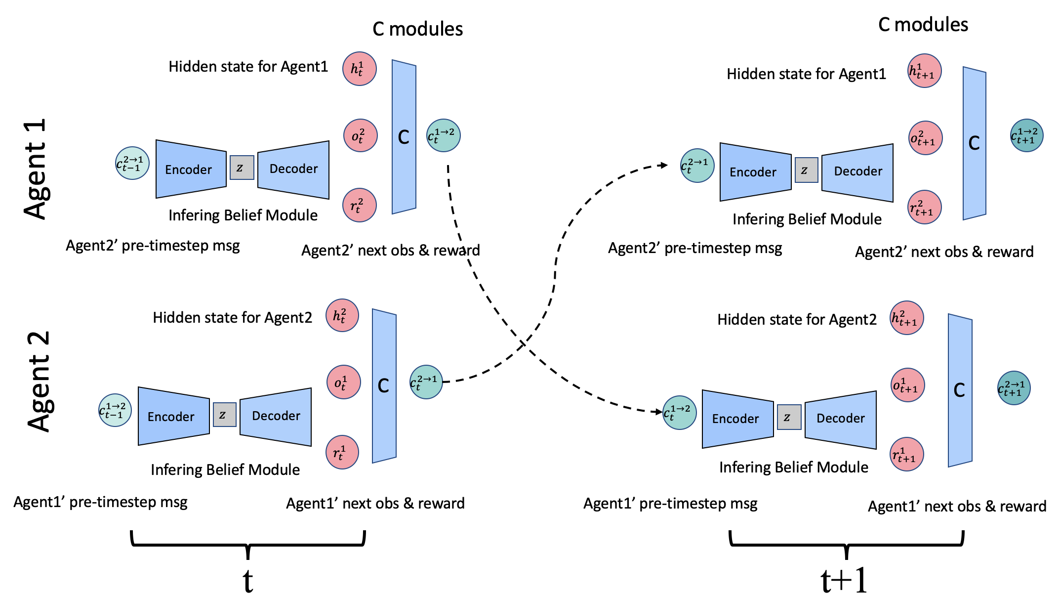
Figure 2: The communication architecture under a multi-agent setting. Suppose we have $N$ agents, each of them at time $t$ receives the observation $o_{t}$ and the communication message $c_{t}$. The message is reconstructed by a VAE component which takes in and sums up all the other agents’ hidden state.

Specifically, our architecture contains three functional modules (see Figure 2 and 3). First, each agent has an inferring beliefs module (IBM), maintaining its interpretation and modelling others under uncertainty. And a communication module (C module) learns how to compress and encode an agent’s observation and belief into compact codes. Finally, a policy module makes decisions based on the interpretation of the ongoing communication. We put forward three contributions: 1) We propose a generative module to infer other agents’ beliefs; 2) We give the agents the ability to learn how to generate effective (concise) messages; 3) We showed that our method could learn to reach higher performance with all these functionalities.

2 Related Work

2.1 Modeling Other Agents

Opponent modelling is a popular and promising research direction in multi-agent reinforcement learning (MARL). The unstable nature of the shared MARL environment has encouraged works to integrate other agents’ models into the controlled agent’s policy. By including a belief in the opponent’s behaviour, the uncertainty of the environment is partially relieved during training.

He et al. (He et al., 2016) propose DRON, building a reinforcement learning framework based on DQN, which jointly learns the policy and the opponent modelling conditioned on observations. Zhang et al. (Zhang et al., 2020) takes the model uncertainty into account while trying to make the MARL algorithm more robust. Chrisianos et al. (Christianos et al., 2021) propose SePS where they model other agents’ resulting observation and reward. They do so by pre-training a clustering mechanism. MoT (Machine theory of Mind) (Rabinowitz et al., 2018) creates two latent variables called agent character $m$ and mental state $m_{t}$ to build a belief on other agents. They use past trajectory for updating the character and current trajectory for mental state. Zintgraf et al. (Zintgraf et al., 2021) borrow this machine theory of mind idea and pass it to other agents who use Bayesian inference to obtain the predicted next action. Previous methods require access to the opponent’s information, Papoudakis et al. (Papoudakis & Albrecht, 2020) propose that the agent can reason about others by just accessing its observation.

2.2 Multi-agent RL based on Communication

For multi-agent reinforcement learning, each agent only has partial observation of the environment, leading to difficulty for learning. It’s naturally possible to introduce a communication channel to provide additional information for the agents when they’re learning cooperative or competitive tasks. This leads us to two questions. 1) How can we construct the message? and 2) Who to communicate? For the first question, CommNet (Sukhbaatar et al., 2016) propose a model that can keep a hidden state for each cooperative agent, and the message is the average value of all other agents’ hidden state. The fully-connected network brings lots of computational burden, especially as the number of agents increases, the length of the message could increase exponentially. Also, it becomes more difficult for an agent to filter the informative values among accumulated messages. IC3Net (Singh et al., 2018) add a gate mechanism on the top of CommNet, where another binary action is then generated for determining whether the agent would like to send the message. Vertex Attention Interaction Network (VAIN) (Hoshen, 2017) adds an attentional architecture for multi-agent predictive modeling. Instead of averaging the messages, they put weights in front of each vector.

3 Background

3.1 Markov Games

We formulate our environment as a Markov game (Shapley, 1953; Littman, 1994; Ye et al., 2020) with $N$ agents defined by the following tuple:

$$\mathcal{M}=(S,O_{1}\ldots O_{N},A_{1}\ldots A_{N},T,R_{1}\ldots R_{N}).$$

Here $N$ is the total number of agents. $S$ denotes the states of all agents. $O_{1}\ldots O_{N},A_{1}\ldots A_{N}$ are the sets observations and actions for each agent. $A_{i}$ is action of Agent $i$ sampled from a stochastic policy $\pi_{i}$ and the next state is generated by the state transition function $T:S\times A_{1}\times\ldots\times A_{N}\to S$. At each step, every agent gets a reward according to the state and corresponding action $r_{i}:S\times A_{i}\times\ldots\times A_{N}\to\mathbb{R}$ along with an observation of the system state $o_{i}:S\to O$. The policy of agent $i$ is $\pi_{i}$. The objective for the $i$-th agent is to learn a policy that maximizes the cumulative discounted rewards

$$\mathcal{R}(i):=\mathbb{E}\Big{[}\sum_{t=0}^{T}\gamma^{t}r_{i}^{(t)})\Big{]},$$ (1)

where $\gamma\in(0,1)$ is the discount factor and $r_{i}^{(t)}$ is the reward received at the $t$-th step.

3.2 Variational Autoencoders

Variational auto-encoder (VAE) is a generative model. It can learn a density function $p(z|x)$, where $z$ is a normally distributed latent variable, $x$ is the given input from dataset $X$. The true posterior distribution $p_{\theta}(\mathbf{z}|\mathbf{x})$ is unknown, so the goal of VAE is to approximate a distribution $q_{\phi}(\mathbf{z}|\mathbf{x})$ which is parametrized by multilayer perceptrons (MLPs). VAEs also use a MLP to approximate $p_{\theta}(x|z)$. The KL-divergence between two is following:

$$D_{KL}(q_{\phi}(\mathbf{z}|\mathbf{x}\|p_{\theta}(\mathbf{z}|\mathbf{x})=logp_{\theta}(\mathbf{x})+D_{KL}(q_{\phi}(\mathbf{z}|\mathbf{x})\parallel p_{\theta}(\mathbf{z}))$$

$$-\mathbf{E}_{z\sim q_{\phi}(\mathbf{z}|\mathbf{x})}logp_{\theta}(\mathbf{x}|\mathbf{z}),$$

which is equal to

$$logp_{\theta}(\mathbf{x})-D_{KL}(q_{\phi}(\mathbf{z}|\mathbf{x}\|p_{\theta}(\mathbf{z}|\mathbf{x})=$$

$$\mathbf{E}_{z\sim q_{\phi}(\mathbf{z}|\mathbf{x})}logp_{\theta}(\mathbf{x}|\mathbf{z})-D_{KL}(q_{\phi}(\mathbf{z}|\mathbf{x})\parallel p_{\theta}(\mathbf{z})).$$

The right side of the equation is called the evidence lower bound (ELBO). Since the second term of the left side is equal or larger than zero, we can get the following inequation:

$$logp_{\theta}(\mathbf{x})\geq\\ \mathbf{E}_{z\sim q_{\phi}(\mathbf{z}|\mathbf{x})}logp_{\theta}(\mathbf{x}|\mathbf{z})-D_{KL}(q_{\phi}(\mathbf{z}|\mathbf{x})\parallel p_{\theta}(\mathbf{z})),$$

so minimising the loss function is equivalent to maximize the ELBO. The density forms of $p(\mathbf{z})$ and $q_{\phi}(\mathbf{z}|\mathbf{x})$ are chosen to be multivariate Gaussian distribution. The empirical objective of the VAE is

$$\begin{gathered}L_{VAE}(\theta,\phi)=-\mathbf{E}_{z\sim q_{\phi}(\mathbf{z}|\mathbf{x})}logp_{\theta}(\mathbf{x}|\mathbf{z})+D_{KL}(q_{\phi}(\mathbf{z}|\mathbf{x})\parallel p_{\theta}(\mathbf{z})),\\ \theta^{*},\phi^{*}=arg\min_{\theta,\phi}L_{VAE}.\end{gathered}$$

The recognition and generative models are parametrised using multilayer perceptrons (MLPs).

4 Belief Embedded Communication

Most opponent modeling methods require direct access of other agents’ information (Papoudakis & Albrecht, 2020) or history of trajectories (He et al., 2016; Raileanu et al., 2018; Li & Miikkulainen, 2018). To lean close to real-life situations, in our hypothesis, agents can only build their beliefs by conversing with each other. Hence, we want to enable every single agent to comprehend and send the latent messages. Via the information exchange, they also learn to recursively reason, wherein they are making decisions based on the knowledge of what the opponent would do based on how they would behave (Wen et al., 2019).

4.1 Inferring Belief Module

Just as the human brain has an area for language processing to understand other agent’s conversation, we construct a similar functional module in our framework. Essentially, we utilise a VAE (Variational Auto Encoder) to represent the belief module and model the agents’ motivation. The message embeds other agents’ future states including represented by following observation and rewards. Using this module, an agent can decode intentions from other agents’ embedded messages in a decentralised manner instead of direct access to other agents’ states.

In addition, every human understands language in the real world using their own implicit model of comprehension. So unlike prior methods, the trained VAE model is not shared by all the agents. We maintain an IBM (Inferring Belief Module) for each agent, i.e., they interpret the received message.

The encoder $q$ and decoder $p$ of VAE are parametrized by $\phi$ and $\theta$ respectively. The input of the encoder are others’ embedded message $c_{t}$ at timestep $t$ which is a $C\times(N-1)$ shape tensor. $C$ is the length of communication vector, $N$ is the total number of agents. We assume each agent can faithfully receive others message without any information loss. The output of the encoder is a $m$-dimensional Gaussian distribution $N(z;\mu,\sigma^{2})$. The decoder predicts the $p(x_{t+1}|z)$, where $x_{t+1}=(o_{t+1},r_{t+1})$ is the next observation and reward.

The agents’ beliefs can be projected to the latent space $Z$ by $q_{\phi}(z|c_{t})$ and $p_{\theta}(z|x_{t+1})$. Hence the objective is to optimize $D_{KL}(q_{\phi}(z|c_{t})\parallel p_{\theta}(z|x_{t+1}))$. Since $p(x_{t+1})$ is intractable, it’s equal to optimize evidence lower bound (ELBO) which we derive as following:

$$\begin{split}logp(x_{t+1})\geq\mathbb{E}_{q_{\theta}\sim(z|c_{t})}[logp_{\theta}(x_{t+1}|z)\\ -D_{KL}(q_{\theta}(z|c)\parallel p(z))]\end{split}$$ (2)

We collect the trajectories and messages for certain period of time. The IBM of each agent is trained independently. While training, the trajectories of all agents are collected and saved to a buffer, for every 50 epochs, we train VAEs 10 times.

4.2 Policy and Message Generation Module

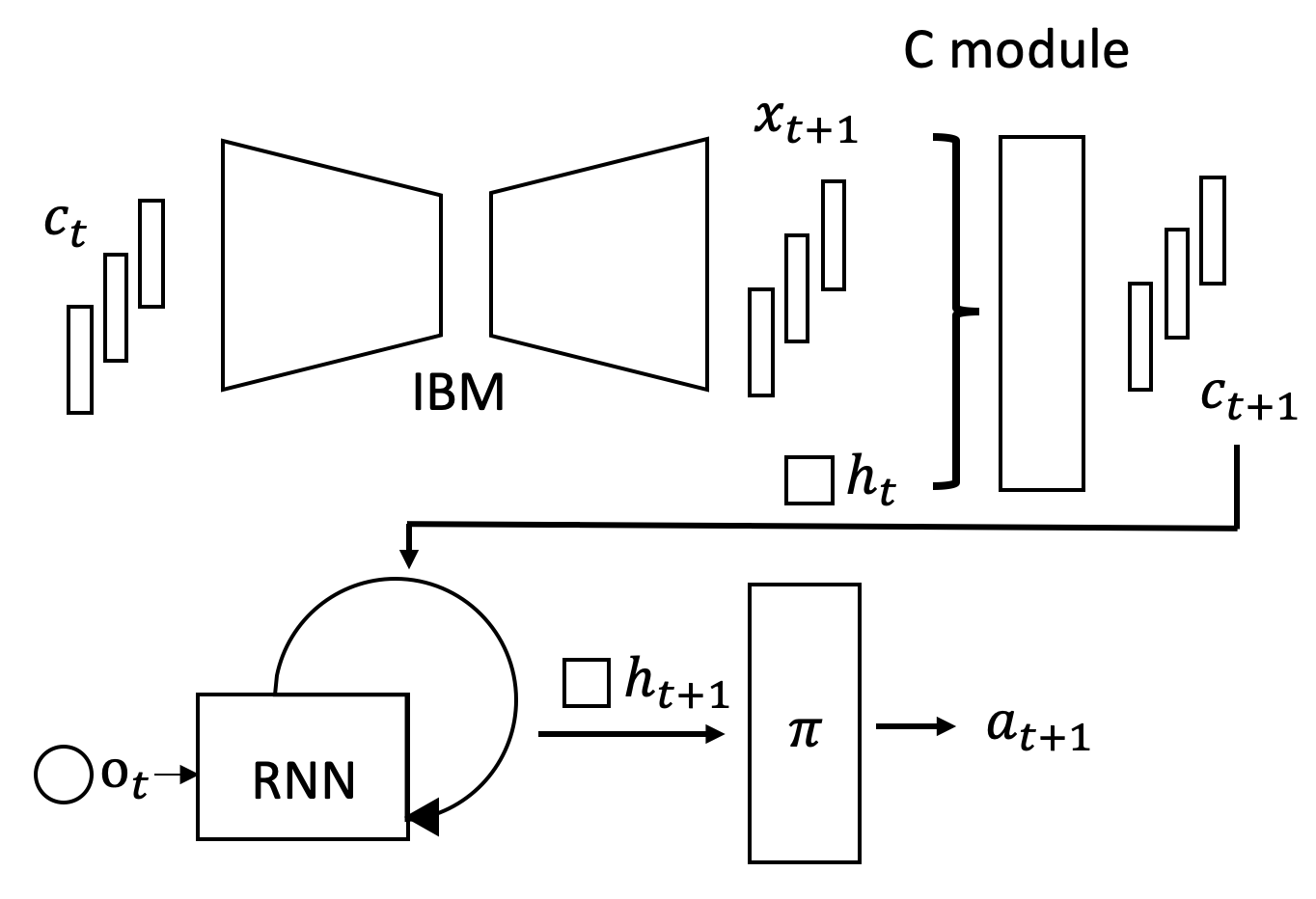
Figure 3: The variable flow graph of Message and policy generation module. The strip shaped bars and squares are the vectors flow in and out the modules. The message pass through the IBM (Intention Belief Module) to get the predictions of other agent’s intention named $x_{t+1}$. C module then utilize the predictions and agent’s own hidden state to generate next timestep’s communication vector $c_{t+1}$. The policy module add in observation and passing through a RNN and policy network outputing action $a_{t+1}$.

For agents, the policy module takes in the observation from environments and combines the beliefs of others’ intentions predicted by previous IBM. It outputs the message delivered to others and subsequent actions agents will take.

The new generated communication vector is continuous, it’s aggregated by all the IBM predictions that represent the agent’s belief and agent’s own hidden state (see Figure 3). For agent $j$, $c^{j}_{t+1}$ is the generated message to others at timestep $t$ shown as following:

$$c^{j}_{t+1}=\frac{1}{N-1}C(\sum_{j=1}^{N-1}x_{t+1}^{j}+h_{t})$$

$$x_{t+1}^{j}=IBM(c^{j}_{t})$$

$$h_{t+1}=RNN(o_{t}+c_{t+1}).$$

The message generation module $C$ is parametrised by a fully connected neural network. Previous IBM(Inferring Belief Module) decodes $x_{t+1}^{j}$. There is no importance factor multiplied by each vector. We also prepare an RNN module to keep track of the agent’s hidden state like (Singh et al., 2018; Sukhbaatar et al., 2016). Next timestep’s hidden state $h_{t+1}$ is generated by this recurrent module where the input is current step’s observation $o_{t}$ and the new generated communication $c_{t+1}$ The next action is generated using policy network implemented as fully-connected neural network $a^{j}_{t}=\pi(h_{t})$.

4.3 Implementation

0:  Total episode number $E$, Duration of each episode $T$, Number of agents $N$. VAE training interval $I$.

1:  Initialize policy $\pi_{0}$, VAE models’ parameter $\theta,\phi$, RNN module. Initialize memory buffer $\mathbf{B}$ Initialize IBM’s $N$ replay buffer $\mathbf{D}=\{D^{0},\cdots,D^{N}\}$

2:  for $k=0,\ldots,E-1$ do

3:     Play an episode using current policy $\pi_{k}$.

4:     add trajectory $\tau_{k}$ into memory buffer $\mathbf{B}$

5:     for $j=0,\ldots,N$ do

6:        add $c^{-j}$, $s^{-j}$ and $r^{-j}$ into replay buffer $D^{j}$

7:     end for

8:     Update policy $\pi_{k+1}=\pi_{k}+\beta\nabla_{\theta}{\hat{J}_{\pi}(\pi_{k})}$ and RNN using the data in memory buffer $\mathbf{B}$.

9:     if k is divisible by $I$ then

10:        for $j=0,\ldots,N$ do

11:           Update $\theta,\phi$ using samples from $D^{j}$

12:        end for

13:     end if

14:  end for

15:  return optimal $\pi^{*},\theta^{*},\phi^{*}$

Algorithm 1 Intention Embedded Communication

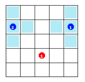
(a) PredatorPrey

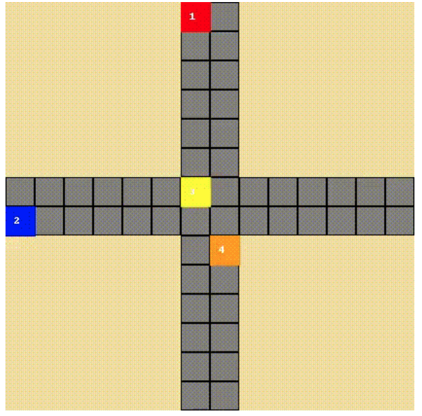
(b) TrafficJunction

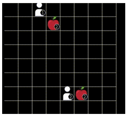
(c) Level-based Foraging

Figure 4: Environments used in our experiment. Left is PredatorPrey Env. The blue circles with numbers represent the predators and the red one is the prey. The azure blocks around the predator illustrate their (limited) visual inputs. The default grid size is $5\times 5$. In our setting, the grid size, number of agents and vision are changeable according to the different difficulty settings. The center is TrafficJunction Env. Each agent represented by colored circles need to pass the crossroads without collision. Their actions are limited to gas and brake. The right is Level-based Foraging, the largest difference of this environment and PredatorPrey is that it requires a level verification while collecting the targets.

As Algorithm 1 shows, we first initialise a policy $\pi_{0}$ and $N$ belief modules, each representing specific agent’s comprehension of the received message. We train the policy learning module and inferring belief module (IBM), separately. Since IBM is trained along with the policy, as the agents’ policy evolves, the comprehension ability updates at set intervals. Specifically, for every $I$ episode, our method collects this period of experience into buffer $\mathbf{D}=\{D^{0},\cdots,D^{N}\}$. For each agent’s buffer $D^{j}$, it contains others’ message $c^{-j}$, next state $s^{-j}$ and reward $r^{-j}$ for training. In the next update iteration, the buffers are emptied because the context between agents is changed. Memory buffer $\mathbf{B}$ collects all the interactions for each step, including the rewards, then the pairs are used to train the policy $\pi$ like standard reinforcement learning methods. By the end, we anticipate that all agents can learn to hear (inferring other’s messages correctly) and speak (generate informative messages) in an efficient way. We follow the centralized training with decentralized execution (CDTE) paradigm.

5 Experiment

The following sections present the experiments where we evaluate our approach in multiple multi-agent environments including PredatorPrey (Singh et al., 2018), TrafficJunction (Koul, 2019) and Level-base Foraging (Papoudakis et al., 2021) showing in Figure 4. These environments require effective coordination between agents. We exhaustively compare our algorithm (IEC) with other state-of-art multi-agent methods in each environment and probe into the different configurations and parameters that may affect the performance. All results presented are averaged over five independent seeds. Our algorithm’s network architecture is kept the same for all runs. The learning rate is $1\times 10^{-3}$ and batch size is $500$. The buffer size for VAE is $4\times 10^{4}$; we trained the VAE every 50 episodes.

5.1 Baselines

We compare our method with following popular multi-agent methods as baselines.

VDN: Value-decomposition Networks (Sunehag et al., 2017) factorize the joint value function into $N$ Q-functions for $N$ agents. Each agent’s value function only relies on its local trajectory.
QMIX: QMIX (Rashid et al., 2018) is a value-based off-policy algorithm that extends the VDN with a constraint that enforces the monotonic improvement.
MADDPG: Multi-Agent Deep Deterministic Policy Gradient (Lowe et al., 2017) use trajectories of all agents to learn a centralized critic. At execution phase, the actors act in decentralized manner.

5.2 PredatorPrey

In the PredatorPrey environment, $N$ predators are assigned to capture the prey. The setting is that only after all predators reach the prey’s location can the reward be given to them. The observation of a given predator is its concatenation of the nearby grid. The actions are discrete options (Forward, Backward, Left, Right, Stale) for all agents. The maximum number of steps for each episode is 20.

The first experiment we conducted is a simple cooperative setting with $5\times 5$ grid as a base map. For every episode, 2 predators and 1 prey are randomly allocated in the grid world. When all the predators reach the prey’s location, they are awarded 5 points. We sum up all predators’s rewards as an indicator of performance. We run experiments for 5 trials with independent seeds. The learning rate for our algorithm and other baselines is 0.001. As shown in Figure 6(a), our algorithm converges speedily compared to others. It uses around half of the interactions compared to the second-best MADDPG.

We then tested our algorithm on various environment settings. Specifically, we follow most settings from (Singh et al., 2018) to construct three levels of difficulty with different agents numbers, grid size and agents’ vision. The details can be found in Table 1. The communication vector length in the three environments is the default 128 lengths.

Agents Num Grid Size Agent’s Vision Easy Version 2 5 0 Medium Version 4 10 1 Hard Version 10 20 1

Table 1: Settings of different versions of the PredatorPrey environment

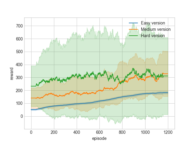
Figure 5: The learning curves of IEC on different difficulty levels of the PredatorPrey Env. It shows that as environment becomes more complicated, the variance notably increases.

As Figure 6(a) shows, when the environment becomes more difficult for the agents, the variance enlarges, since in our setting, we assign the rewards to agents only when all the agents reach the prey’s location. As the number of agents increase and the grid size expands, it’s challenging for them to finish the task in limited time steps.

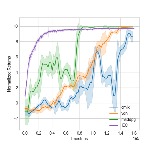
(a) PredatorPrey

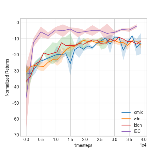
(b) TrafficJunction

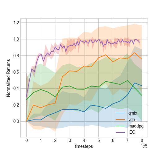
(c) Level-based Foraging

Figure 6: Performance of IEC and other baselines listed in 5.1 during the training protocol. The y-axis is normalized returns and x-axis is the total time steps the algorithm takes. As shown in three subplots, IEC can learn the task faster and achieve higher or equal returns by the end.

We conduct several experiments for investigating the influence of the message size. Our communication consists of the hidden state, and the agent’s beliefs of others. The message generation module concatenates these two together and forwards them to a trainable neural network for the final outputs. The length of the message is adjustable, so in the following experiment, we probe into the influence of the length of the different bits. We conduct experiments with 32, 64 and 128 bits of message and show their training process. As observed in the left plot of Figure 8, the length of the communication vector has a significant influence on policy optimisation. Longer bits can carry more encoded information and facilitates communication between agents.

5.3 Traffic Junction

The traffic junction environment we use references to (Singh et al., 2018) and (Koul, 2019). In this environment, cars move across intersections in which they need to avoid collisions with each other. There are adjustable routes users can set. The number of routes and agents define the three levels of difficulty named easy, medium and hard version.

We first compared our method with other baselines. As Figure 6(b) shows, agents trained by our method can learn to cooperate at a much faster speed and also furnish higher final returns. The other methods are nearly of the same performance. The TrafficJunction environment requires agents to utilise all local observations to get the other agent’s position and intention. This setting brings a great advantage for our method because the belief and cooperation information can be encoded into a message. Under our framework, the negotiation can be reached by mutual recursive reasoning to avoid a collision.

The multi-agent traffic junction environment also has three versions with incremental levels. Table 2 lists the details. Figure 7 shows that the parameters in Table 2 pulls down the converged total reward and brings more variance into cooperation among agents.

Agents Num Grid Size Max Steps Easy Version 5 6 20 Medium Version 14 10 40 Hard Version 20 18 80

Table 2: Settings of different versions TrafficJunction environment

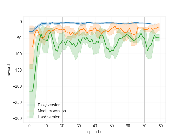
Figure 7: The learning curves of IEC on different difficulty level of TrafficJunction Env.

Same as in the Predator-Prey environment, we want to test our algorithm on different bits of message on the Traffic Junction environment. We can tell from the centre plot of Figure 8 that, unlike the predator-prey environment, the bit-length of information causes disparity in the final performance; in a traffic junction environment, it primarily affects the learning speed.

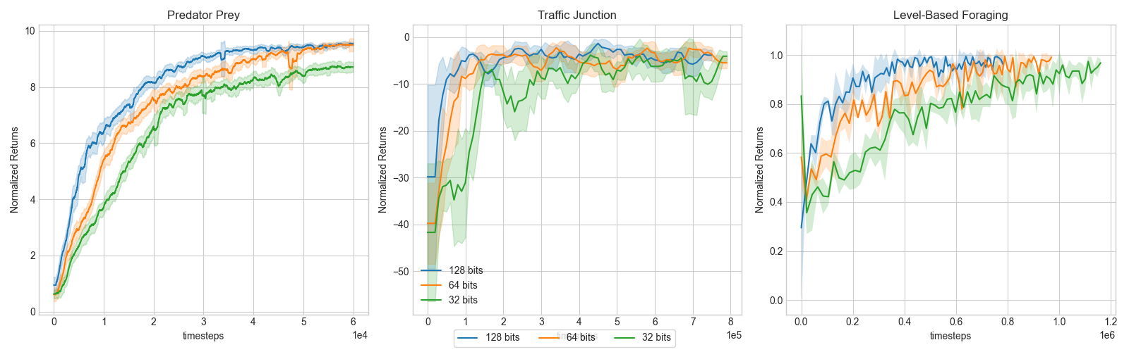
Figure 8: Learning curves with different bits (128,64,32) respectively in three environments. This figure demonstrates that the bit-length (capacity) of the communication vector – which represents the amount of information it can carry – has distinct influence on learning speed. The size of this influence varies across different tasks.

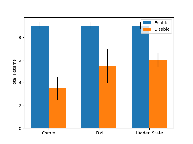
Figure 9: The blue bars are all function enabled IEC with communication vector of size 128 bits. The orange bar is the returns the algorithm can achieve after disabling the corresponding feature.

5.4 Level-based Foraging

Level-based Foraging (LBF) is a multi-agent environment focusing on the coordination of the agents involved (Papoudakis et al., 2021). Compared to the PredatorPrey environment, agents and food in this world are assigned within a level; only when the agent’s level is equal to or higher than a certain limit, can it successfully collect the food, as in Figure 4. The action space contains four directional moves and a loading action. This environment is more challenging than previous ones due to its additional limitations.

Figure 6(c) shows our algorithm obtains higher learning speed and normalised returns than QMIX and VDN. The constraint that only a certain level can elicit pick up of the food decreases the probability that the agents randomly hit the target. This also requires richer observation and more efficient cooperation, like not wasting time collecting the same food. In such a scenario, we can see our intention encoded communication plays a vital role in assisting agents in achieving their goals.

5.5 Ablation Study

This section discusses some key building modules communication, IBM, and hidden state, respectively. They have a significant influence on final performance. We conducted an ablation study by solely disabling these features compared with the fully functional IEC in the PredatorPrey environment. The difficulty level is easy, and the message length stays at 128 bits.

No Communication We analyse the functionality of the communication mechanism. In this setting, agents do not have any exchanges, which means the IBM is also unavailable due to the lack of passing messages; they can only use their observation as input for decision making. Figure 9’s first pair shows that the predator encounters greater total reward loss than the method with fully functional communication.

No IBM For validation of our Inferring Belief Module (IBM)’s functionality, we run one experiment that all predators only receive others’ hidden state as a message, i.e., agents do not exchange each other’s embedded intentions during the experiment. Figure 9’s centre plot shows that without the extra belief inference of other agents’ messages cause about $38\%$ performance decrease.

No Hidden State A hidden state is the vector we use to embed the agent’s previous state using an RNN. Details can be found in Section 4.2. As the right plot of Figure 9 shows, the algorithm reaches around 2/3 returns compared to IEC if the hidden state is missing in a transmitted message. We can see that the compact information of the agent’s state also brings some help to complete the cooperation tasks. But without IBM, it can’t reach maximal returns.

6 Conclusion

This paper proposes IEC framework that can mimic the multiple agent’s natural communication in cooperative tasks. We devise two modules: Infer Beliefs Module (IBM) and Message Generation Module. These modules abstractly represent functional areas in the brain for successful comprehension inference and grammar generation. We also adopt the idea that agents learn the communication and underlying grammar by trial and error (co-evolution). We empirically demonstrated that our algorithm could outperform other multi-agent baselines with a significant gain in data efficiency. Such an algorithm stays robust under various environment settings, like different difficulties and message length. The ablation study also investigates the processes’ key factors and reveals their contribution. In future work, we would like to explore more generative structures like GANs for inferring belief modules.

References

- Christianos et al. (2021) Christianos, F., Papoudakis, G., Rahman, A., and Albrecht, S. V. Scaling multi-agent reinforcement learning with selective parameter sharing. arXiv preprint arXiv:2102.07475, 2021.
- He et al. (2016) He, H., Boyd-Graber, J., Kwok, K., and Daumé III, H. Opponent modeling in deep reinforcement learning. In International conference on machine learning, pp. 1804–1813. PMLR, 2016.
- Hoshen (2017) Hoshen, Y. Vain: Attentional multi-agent predictive modeling. arXiv preprint arXiv:1706.06122, 2017.
- Koul (2019) Koul, A. ma-gym: Collection of multi-agent environments based on openai gym. https://github.com/koulanurag/ma-gym, 2019.
- Langley (2000) Langley, P. Crafting papers on machine learning. In Langley, P. (ed.), Proceedings of the 17th International Conference on Machine Learning (ICML 2000), pp. 1207–1216, Stanford, CA, 2000. Morgan Kaufmann.
- Lazaridou et al. (2016) Lazaridou, A., Peysakhovich, A., and Baroni, M. Multi-agent cooperation and the emergence of (natural) language. arXiv preprint arXiv:1612.07182, 2016.
- Li & Miikkulainen (2018) Li, X. and Miikkulainen, R. Dynamic adaptation and opponent exploitation in computer poker. In Workshops at the Thirty-Second AAAI Conference on Artificial Intelligence, 2018.
- Littman (1994) Littman, M. L. Markov games as a framework for multi-agent reinforcement learning. In Machine learning proceedings 1994, pp. 157–163. Elsevier, 1994.
- Lowe et al. (2017) Lowe, R., Wu, Y., Tamar, A., Harb, J., Abbeel, P., and Mordatch, I. Multi-agent actor-critic for mixed cooperative-competitive environments. arXiv preprint arXiv:1706.02275, 2017.
- Mnih et al. (2015) Mnih, V., Kavukcuoglu, K., Silver, D., Rusu, A. A., Veness, J., Bellemare, M. G., Graves, A., Riedmiller, M., Fidjeland, A. K., Ostrovski, G., et al. Human-level control through deep reinforcement learning. nature, 518(7540):529–533, 2015.
- Mordatch & Abbeel (2018) Mordatch, I. and Abbeel, P. Emergence of grounded compositional language in multi-agent populations. In Thirty-second AAAI conference on artificial intelligence, 2018.
- Papoudakis & Albrecht (2020) Papoudakis, G. and Albrecht, S. V. Variational autoencoders for opponent modeling in multi-agent systems. arXiv preprint arXiv:2001.10829, 2020.
- Papoudakis et al. (2021) Papoudakis, G., Christianos, F., Schäfer, L., and Albrecht, S. V. Benchmarking multi-agent deep reinforcement learning algorithms in cooperative tasks. In Proceedings of the Neural Information Processing Systems Track on Datasets and Benchmarks (NeurIPS), 2021.
- Rabinowitz et al. (2018) Rabinowitz, N., Perbet, F., Song, F., Zhang, C., Eslami, S. A., and Botvinick, M. Machine theory of mind. In International conference on machine learning, pp. 4218–4227. PMLR, 2018.
- Raileanu et al. (2018) Raileanu, R., Denton, E., Szlam, A., and Fergus, R. Modeling others using oneself in multi-agent reinforcement learning. In International conference on machine learning, pp. 4257–4266. PMLR, 2018.
- Rashid et al. (2018) Rashid, T., Samvelyan, M., Schroeder, C., Farquhar, G., Foerster, J., and Whiteson, S. Qmix: Monotonic value function factorisation for deep multi-agent reinforcement learning. In International Conference on Machine Learning, pp. 4295–4304. PMLR, 2018.
- Shapley (1953) Shapley, L. S. Stochastic games. Proceedings of the national academy of sciences, 39(10):1095–1100, 1953.
- Silver et al. (2016) Silver, D., Huang, A., Maddison, C. J., Guez, A., Sifre, L., Van Den Driessche, G., Schrittwieser, J., Antonoglou, I., Panneershelvam, V., Lanctot, M., et al. Mastering the game of go with deep neural networks and tree search. nature, 529(7587):484–489, 2016.
- Singh et al. (2018) Singh, A., Jain, T., and Sukhbaatar, S. Learning when to communicate at scale in multiagent cooperative and competitive tasks. arXiv preprint arXiv:1812.09755, 2018.
- Sukhbaatar et al. (2016) Sukhbaatar, S., Fergus, R., et al. Learning multiagent communication with backpropagation. Advances in neural information processing systems, 29:2244–2252, 2016.
- Sunehag et al. (2017) Sunehag, P., Lever, G., Gruslys, A., Czarnecki, W. M., Zambaldi, V., Jaderberg, M., Lanctot, M., Sonnerat, N., Leibo, J. Z., Tuyls, K., et al. Value-decomposition networks for cooperative multi-agent learning. arXiv preprint arXiv:1706.05296, 2017.
- Tian et al. (2019) Tian, Z., Wen, Y., Gong, Z., Punakkath, F., Zou, S., and Wang, J. A regularized opponent model with maximum entropy objective. arXiv preprint arXiv:1905.08087, 2019.
- Tian et al. (2020) Tian, Z., Zou, S., Davies, I., Warr, T., Wu, L., Ammar, H. B., and Wang, J. Learning to communicate implicitly by actions. In Proceedings of the AAAI Conference on Artificial Intelligence, volume 34, pp. 7261–7268, 2020.
- Wen et al. (2019) Wen, Y., Yang, Y., Luo, R., Wang, J., and Pan, W. Probabilistic recursive reasoning for multi-agent reinforcement learning. arXiv preprint arXiv:1901.09207, 2019.
- Ye et al. (2020) Ye, G., Lin, Q., Juang, T.-H., and Liu, H. Collision-free navigation of human-centered robots via markov games. In 2020 IEEE International Conference on Robotics and Automation (ICRA), pp. 11338–11344. IEEE, 2020.
- Zhang et al. (2020) Zhang, K., Sun, T., Tao, Y., Genc, S., Mallya, S., and Basar, T. Robust multi-agent reinforcement learning with model uncertainty. In NeurIPS, 2020.
- Zintgraf et al. (2021) Zintgraf, L., Devlin, S., Ciosek, K., Whiteson, S., and Hofmann, K. Deep interactive bayesian reinforcement learning via meta-learning. arXiv preprint arXiv:2101.03864, 2021.