Correlated quantization for distributed mean estimation and optimization

Abstract

We study the problem of distributed mean estimation and optimization under communication constraints. We propose a correlated quantization protocol whose leading term in the error guarantee depends on the mean deviation of data points rather than only their absolute range. The design doesn’t need any prior knowledge on the concentration property of the dataset, which is required to get such dependence in previous works. We show that applying the proposed protocol as a sub-routine in distributed optimization algorithms leads to better convergence rates. We also prove the optimality of our protocol under mild assumptions. Experimental results show that our proposed algorithm outperforms existing mean estimation protocols on a diverse set of tasks.

1 Introduction

Large-scale machine learning systems often require the distribution of data across multiple devices. For example, in federated learning (Kairouz et al., 2021), data is distributed across user devices such as cell phones, and the machine learning models are trained with adaptive stochastic gradient descent methods or their variations like federated averaging (McMahan et al., 2017). Such algorithms require multiple rounds of communication between the devices and the centralized server. At each round, the devices send model updates to the server, and the server aggregates the data and outputs a new model.

In many scenarios like federated learning, the data from devices are sent to the server over wireless channels. Communication between devices and the server, especially the uplink communication, is a bottleneck. This has resulted in a series of works on compression and quantization methods to reduce the communication cost (Konečnỳ et al., 2016; Lin et al., 2018; Alistarh et al., 2017).

At the heart of these algorithms is the distributed mean estimation protocol where each client has a model update (in the form of a vector). Each client compresses its update and transmits the compressed version to the server. The server then decompresses and aggregates the updates to approximate the mean of the updates. In this work, we study the problem of distributed mean estimation and provide the first algorithm whose leading term of the error depends on the mean deviation of the inputs rather than only their absolute range without additional side information. We then use these results to provide improved convergence guarantees for distributed optimization protocols. Before we proceed further, we need a few definitions.

Distributed mean estimation.

Let $\mathcal{X}\subset\mathbb{R}^{d}$ be the input space and $x^{n}=x_{1},x_{2},\ldots,x_{n}$ be the $n$ data points where each $x_{i}\in\mathcal{X}$. For most results, we assume $\mathcal{X}=\mathbb{B}^{d}(R)\stackrel{{\scriptstyle\mathrm{def}}}{{=}}\{x\in\mathbb{R}^{d}\mid\|x\|_{2}\leq R\}$, the $\ell_{2}$ ball of radius $R$. We denote the mean of the vectors as

$${\bar{x}}=\frac{1}{n}\sum^{n}_{i=1}x_{i}.$$

In compression, these $x_{i}$s are encoded at the clients and then decoded at the server (Mayekar and Tyagi, 2020). $Q_{i}$, the quantizer (encoder) at client $i$ is a (possibly randomized) mapping from $\mathcal{X}\to\mathcal{Y}$, where $\mathcal{Y}$ is the quantized space. With the slight abuse of notation let $Q^{n}=Q_{1},Q_{2},\ldots Q_{n}$, be the set of quantizers. Each client encodes $x_{i}$ and sends $Q_{i}(x_{i})$ to the server. The server then decodes $Q^{n}(x^{n})$ to get an estimate of the mean $\hat{x}$. Following earlier works (Suresh et al., 2017; Mayekar and Tyagi, 2020), we measure the performance of the quantizer in terms of mean squared error,

$$\mathcal{E}(Q^{n},x^{n})\stackrel{{\scriptstyle\mathrm{def}}}{{=}}\mathbb{E}\|\hat{x}-{\bar{x}}\|_{2}^{2},$$

where the expectation is over the public and private randomness of the algorithm.

Distributed optimization.

We consider solving the following optimization task using distributed stochastic gradient descent (SGD) methods. Let $F:\mathbb{R}^{d}\rightarrow\mathbb{R}$ be an objective function and the goal is to minimize the $F$ over an $\ell_{2}$-bounded space $\Omega\stackrel{{\scriptstyle\mathrm{def}}}{{=}}\{w\in\mathbb{R}^{d}\mid\|w\|_{2}\leq D\}.$ Motivated by the federated learning setting, we assume there are $T$ rounds of communication. At round $t$, a set of $n$ clients is involved, and each of them has access to a stochastic gradient oracle of $F$, denoted by ${g}$.

In distributed SGD, after selecting a random initialization $w_{0}\in\Omega$, at round $t$, each client queries the oracle at $w_{t}$. Under communication constraints, users must quantize their obtained gradient with limited bits and send it to the server. The server then uses these quantized messages to estimate the true gradient of $F(w)$, which is the average of local gradients. We denote this estimate as $\widehat{\nabla}F(w_{t})$. The server then updates the parameter with some learning rate

$$w_{t+1}=w_{t}-\eta_{t}\widehat{\nabla}F(w_{t}),$$

and projects it back to $\Omega$, which is sent to all clients in the next round.

Under smoothness assumptions on $F$, standard results in optimization, e.g., Bubeck (2015), allow us to obtain convergence results given mean squared error guarantees for the mean estimation primitive $\mathbb{E}[(\widehat{\nabla}F(w_{t})-\nabla F(w_{t}))^{2}]$. Hence we will focus on analyzing error guarantees on the mean estimation task and discuss their implications on distributed optimization.

2 Related Works

The goal of distributed mean estimation is to estimate the empirical mean without making distributional assumptions of the data. This is different from works estimating the mean of the underlying distributional model (Zhang et al., 2013; Garg et al., 2014; Braverman et al., 2016; Cai and Wei, 2020; Acharya et al., 2021). To achieve guarantees in terms of the deviation of the data, these techniques rely on the distributional assumption, which is not applicable in our setting.

The classic algorithm for this problem is stochastic scalar quantization, where each dimension of the data is stochastically quantized to one of the fixed values (such as 0 or 1 in stochastic binary quantization). This provides an unbiased estimation with reduced communication cost. It has been shown that adding random rotation reduces quantization error (Suresh et al., 2017) and variable-length coding provides the near-optimal communication-error trade-off (Alistarh et al., 2017; Suresh et al., 2017). Many variants and improvements of the scalar quantization algorithms exist. For example, Terngrad (Wen et al., 2017) and 3LC (Lim et al., 2019) use a three-level stochastic quantization strategy. SignSGD uses the sign of the coordinate of gradients rather than quantizing it (Bernstein et al., 2018). 1-bit SGD uses error-feedback as a mechanism to reduce the error in quantization (Seide et al., 2014); error-feedback (Stich and Karimireddy, 2020) is orthogonal to our work and can be potentially used in combination. Mitchell et al. (2022) proposes to learn the quantizer leveraging data distribution across the clients using rate-distortion theory. Vargaftik et al. (2021b) proposes DRIVE, an improvement of the random rotation method by replacing the stochastic binary quantization with the sign operator. This method is shown to outperform other variants of scalar quantization. Recent work of Vargaftik et al. (2021a) generalizes DRIVE to handle any communication budget. Other techniques include Sparsified SGD (Stich et al., 2018) and sketching based approaches (Ivkin et al., 2019).

Beyond scalar quantization, vector quantization may lead to higher worst-case communication cost (Gandikota et al., 2021). Kashin’s representation has been used to quantize a $d$-dimensional vector using less than $d$ bits (Caldas et al., 2018b; Chen et al., 2020; Safaryan et al., 2021). Davies et al. (2021) use the lattice quantization method which will be discussed below.

More broadly, our work is also related to non-quantization methods to improve the communication cost of distributed mean estimation, often under the context of distributed optimization. Examples include gradient sparsification (Aji and Heafield, 2017; Lin et al., 2018; Basu et al., 2019) and low rank decomposition (Wang et al., 2018; Vogels et al., 2019). These methods require assumptions of the data such as high sparsity or low rank. The idea of using correlation between local compressors has also been considered in Szlendak et al. (2021) for gradient sparsification. The paper uses shared randomness to select coordinates without-replacement across clients, which is also shown to be advantageous to independent masking. Without compression, Yun et al. (2022) studies the effect of randomness in local data reshuffling. The paper shows that for both local and mini-batch SGD, sampling indices without-replacement can outperform sampling with-replacement counterparts in certain regimes.

Perhaps closest to our work is that of Davies et al. (2021); Mayekar et al. (2021), who proposed algorithms with error that depends on the variance of the inputs. However, these works all need certain side information about the inputs, and deviate from our work in two ways: first in Davies et al. (2021), the clients need to know the input variance. Secondly, both Davies et al. (2021); Mayekar et al. (2021) require the server to know one of the client values to a high accuracy. Finally, their information theoretically optimal algorithm is not computationally efficient, and their efficient algorithm is sub-optimal in logarithmic factors. We note that correlated random variables are also used in Mayekar et al. (2021). They use the same random variable to quantize both the input vector and the side information. This is very different from our proposed approach, which generates correlated random variables which are used for different input vectors.

3 Our Contributions

We propose correlated quantization that only requires a simple modification in the standard stochastic quantization algorithm. Correlated quantization uses shared randomness to introduce correlation between local quantizers at each client, which results in improved error bounds. In the absence of shared randomness, it can be simulated by the server sending a seed to generate randomness to all the clients. We first state the error guarantees below.

In one dimension, if all values lie in the range $[l,r]$, the error of standard stochastic quantization with $k$ levels scales as (Suresh et al., 2017)

$$\mathcal{O}\left(\frac{(r-l)^{2}}{nk^{2}}\right).$$

In this work, we show that the modified algorithm (Algorithm 2) has error that scales as

$$\mathcal{O}\left(\min\left(\frac{\sigma_{\text{md}}(r-l)}{nk},\frac{(r-l)^{2}}{nk^{2}}\right)+\frac{(r-l)^{2}}{n^{2}k^{2}}\right),$$

where $\sigma_{\text{md}}$ is the empirical mean absolute deviation of points defined below:

$$\sigma_{\text{md}}\stackrel{{\scriptstyle\mathrm{def}}}{{=}}\frac{1}{n}\sum_{i=1}^{n}\left|x_{i}-{\bar{x}}\right|.$$ (1)

Informally, $\sigma_{\text{md}}$ models how concentrated the data points are. Compared to other commonly used concentration measures, such as worst-case deviation (Mayekar et al., 2021)

$$\sigma_{\text{max}}\stackrel{{\scriptstyle\mathrm{def}}}{{=}}\max_{i}|x_{i}-{\bar{x}}|,$$

and standard deviation (Davies et al., 2021)

$$\sigma\stackrel{{\scriptstyle\mathrm{def}}}{{=}}\sqrt{\frac{1}{n}\sum_{i=1}^{n}\left(x_{i}-{\bar{x}}\right)^{2}},$$

it holds that $\sigma_{\text{md}}\leq\sigma\leq\sigma_{\text{max}}\leq r-l$. Hence our result implies bounds in terms of these concentration measures as well.

When $\sigma_{\text{md}}<\frac{r-l}{k}$, i.e., the data points are “close” to each other, the proposed algorithm has smaller error than stochastic quantization. Notice that it was shown in previous works that better error guarantees can be obtained when the data points have better concentration properties. However these works rely on knowing a bound on the concentration radius (Davies et al., 2021) or side information such as a crude bound on the location of the mean (Davies et al., 2021; Mayekar et al., 2021). Different from the above, our proposed scheme doesn’t require any side information. Moreover, we remark that our proposed scheme only requires a simple modification of how randomness is generated in the standard stochastic quantization algorithm while these algorithms are based on sophisticated encoding schemes based on the availability of prior information.

Lower bound.

When $\sigma_{\text{md}}$ is small, we further show that in the one-dimensional case, our obtained bound is optimal for any $k$-interval quantizers (see Definition 1), which is commonly used in many state-of-the art compression algorithms in distributed optimization including stochastic quantization and our proposed algorithm. Moreover, when each client is only allowed to use one bit (or constant bits), the obtained bound is information-theoretically optimal for any quantizers.

Extension to higher dimensions.

In high dimensions, if all values lie in $\mathbb{B}^{d}(R)$, the error of the min-max optimal algorithms with $k$ levels of quantization scales as (Suresh et al., 2017)

$$\tilde{\mathcal{O}}\left(\frac{R^{2}}{nk^{2}}\right).$$

We show that an improvement similar to the previous result:

$$\tilde{\mathcal{O}}\left(\min\left(\frac{\sigma^{d}_{\text{md}}R}{nk},\frac{R^{2}}{nk^{2}}\right)+\frac{R^{2}}{n^{2}k^{2}}\right),$$

where $\sigma^{d}_{\text{md}}$ is the average $\ell_{2}$ distance between data points,

$$\sigma^{d}_{\text{md}}=\frac{1}{n}\sum^{n}_{i=1}\|x_{i}-{\bar{x}}\|_{2}.$$ (2)

Similar to the one-dimensional case, it can be shown that $\sigma^{d}_{\text{md}}$ is upper bounded by $\max_{i}\|x_{i}-{\bar{x}}\|_{2}$ and $(\frac{1}{n}\sum_{i=1}^{n}\|x_{i}-{\bar{x}}\|_{2}^{2})^{1/2}$. And hence the same bound holds for these measures as well.

We note that our dependence on standard deviation is linear. This coincides with the results of Mayekar et al. (2021) for mean estimation with side information. While the results of one are not directly applicable to the other, understanding the two results in the high-dimensional case remains an interesting direction to explore.

Distributed optimization.

Turning to the task of distributed optimization, the proposed mean estimation algorithm can be used as a primitive in distributed SGD algorithm. Following stochastic optimization literature, we assume the gradient oracle $g$ satisfies $\forall w\in\Omega$,

• Unbiasedness: $\mathbb{E}[{g}(w)]=\nabla F(w)$.

• Lipschitzness: $\|{g}(w)\|_{2}\leq R$.

• Bounded variance: $\mathbb{E}[\|{g}(w)-\nabla F(w))\|_{2}^{2}]\leq\sigma^{2}$.

We also assume that the function is convex and smooth. A function $F$ is $H$-smooth, if for all $w,w^{\prime}\in\Omega$,

$$\|\nabla F(w)-\nabla F(w^{\prime})\|_{2}\leq H\|w-w^{\prime}\|_{2}.$$

Using standard results on smooth convex optimization (e.g., Theorem 6.3 in Bubeck (2015)) and estimation error guarantee in Corollary 1, we obtain the following bound.

Theorem 1.

Suppose the objective function $F(w)$ is convex and $H$-smooth, using correlated quantization with $k=\sqrt{d}$ levels as the mean estimation primitive, distributed SGD with $T$ rounds and learning rate $\frac{1}{H+1/\eta}$ yields

$$\mathbb{E}\left[F\left(\frac{1}{T}\sum_{t=1}^{T}w_{t}\right)\right]-\min_{w\in\Omega}F(w)\leq\left(H+\frac{1}{\eta}\right)\frac{D^{2}}{T}+\frac{\eta\triangle^{2}}{2},$$

where $\eta>0$ and $\triangle^{2}=\mathcal{O}\left(\frac{\sigma R}{n}+\frac{R^{2}}{n^{2}}\right)$. Moreover, each client only needs to send $\Theta(d)$ bits (constant bits per dimension) in each round.

Optimization algorithms based on stochastic rounding (Alistarh et al., 2017; Suresh et al., 2017) has convergence rate of the same form with $\triangle^{\prime 2}=\mathcal{O}\left(\frac{R^{2}}{n}\right)$ under the same communication complexity. Notice that the mean squared error (and therefore the convergence rate) we obtain is always better than that of the classic stochastic quantization algorithm, and when $\sigma<R$ the new algorithm gives faster convergence. This corresponds to the case where the clients’ local gradients are better concentrated than their absolute range, which is a mild assumption.

4 A Toy Example

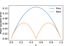
Figure 1: Mean squared error for the toy problem.

Before we proceed further, we motivate our result with a simple example. Suppose there are $n$ devices and device $i$ has $x_{i}\in[0,1]$. Further, let’s consider the simple scenario in which each client can only send one bit i.e., $Q_{i}$ can take only two values. The popular algorithm for mean estimation is stochastic quantization, in which client $i$ sends $Q_{i}(x_{i})$ given by

$$Q_{i}(x_{i})=\begin{cases}1\text{ with probability }x_{i},\\ 0\text{ with probability }1-x_{i}.\end{cases}$$ (3)

Notice that $Q_{i}(x_{i})$ takes only two values and the server computes the mean by computing their average

$$\hat{x}=\frac{1}{n}\sum^{n}_{i=1}Q_{i}(x_{i}).$$

We first note that $Q_{i}(x_{i})$ is unbiased

$$\mathbb{E}[\hat{x}]={\bar{x}}.$$

The mean squared error of this protocol is

$$\mathcal{E}(Q^{n},x^{n})=\frac{1}{n^{2}}\sum^{n}_{i=1}x_{i}(1-x_{i}).$$

To motivate our approach, we consider the special case when $n=2$ and further assume $x_{1}=x_{2}=x$. In this case, the mean squared error of the stochastic quantizer is

$$\mathcal{E}(Q^{2},x^{2})=\frac{x(1-x)}{2}.$$ (4)

The key insight of correlated quantization is that if the first client rounds up its value, the second client should round down its value to reduce the mean squared error. To see this, we first rewrite the original stochastic quantization $Q_{i}$ slightly differently. For each $i$, let $U_{i}$ be an independent uniform random variable in the range $[0,1]$. Then we can rewrite $Q_{i}$ as

$$Q_{i}(x_{i}) =1_{U_{i}<x_{i}}.$$

To see the equivalence of the above definition and (3), observe that the probability of $U_{i}<x_{i}$ is $x_{i}$. Hence $1_{U_{i}<x_{i}}$ is one with probability $x_{i}$ and zero otherwise.

For the special case of $n=2$, we propose to modify the estimator by making $U_{i}$s dependent on each other. In particular, let $U_{1}$ be a uniform random variable in the range $[0,1]$ and let $U_{2}=1-U_{1}$. This can be implemented using shared randomness. Let the modified estimator be as before

$$Q^{\prime}_{i}(x_{i}) =1_{U_{i}<x_{i}}.$$

Since $Q_{i}$ is an unbiased estimator, $Q^{\prime}_{i}$ is also an unbiased estimator. We now compute the mean squared error of $Q^{\prime}$

$$\mathcal{E}(Q^{\prime 2},x^{2}) =\mathbb{E}\left[\left(\frac{Q^{\prime}_{1}(x_{1})+Q^{\prime}_{2}(x_{2})}{2}\right)^{2}\right]-x^{2}$$

$$=\frac{1}{4}\mathbb{E}\left[\left(1_{U_{1}<x}+1_{1-U_{1}<x}\right)^{2}\right]-x^{2}$$

$$=\frac{1}{4}\mathbb{E}\left[1_{U_{1}<x}+1_{1-U_{1}<x}+2\cdot 1_{U_{1}<x}1_{1-U_{1}<x}\right]-x^{2}$$

$$=\frac{1}{4}\mathbb{E}\left[1_{U_{1}<x}+1_{1-U_{1}<x}+2\cdot 1_{1-x<U_{1}<x}\right]-x^{2}$$

$$=\frac{1}{4}\left(x+x+2\max(2x-1,0)\right)-x^{2}$$

$$=\frac{x}{2}+\max\left(x-\frac{1}{2},0\right)-x^{2}.$$

We plot the mean squared error of the original quantizer $Q$ and the new quantizer $Q^{\prime}$ in Figure 1. Observe that the above mean squared error is uniformly upper bounded by the mean squared error of the original quantizer (4). Our goal is to propose a similar estimator for $n$ devices, in $d$ dimensions, that has uniformly low error compared to $Q$ even when the devices have different values of $x_{i}$.

5 Correlated Quantization in One Dimension

We first extend the above idea and provide a new quantizer for bounded scalar values. For simplicity, we first assume each $\mathcal{X}=[0,1]$. Recall that the goal is to estimate $\frac{1}{n}\sum^{n}_{i=1}x_{i}.$ Let $Q_{i}(x_{i})$ be some quantization of $x_{i}$. We approximate the average by $\frac{1}{n}\sum^{n}_{i=1}Q_{i}(x_{i}).$ As we discussed in the previous section, we propose to use

$$Q_{i}(x_{i}) =1_{U_{i}<x_{i}},$$

where $U_{i}$s are uniform random variables between zero and one, but are now correlated across the clients. We generate $U_{i}$s as follows. Let $\pi$ denote a random permutation of $\{0,1,2,\ldots,n-1\}$. Let $\pi_{i}$ denote the $i^{\text{th}}$ value of this permutation. Let $\gamma_{i}$ is a uniform random variable between $[0,1/n)$. With these definitions, we let

$$U_{i}=\frac{\pi_{i}}{n}+\gamma_{i}.$$

Observe that for each $i$, $U_{i}$ is a uniform random variable over $[0,1]$. However, they are now correlated across clients. Hence the quantizer can be written as

$$Q_{i}(x_{i})=1_{\frac{\pi_{i}}{n}+\gamma_{i}<x_{i}}.$$

We illustrate why this quantizer is better with an example. If all clients have the same value $s/n,s\in\{0,1,\ldots,n\}$, the new quantizer can be written as

$$\frac{1}{n}\sum^{n}_{i=1}Q_{i}(s/n) =\frac{1}{n}\sum^{n}_{i=1}1_{\frac{\pi_{i}}{n}+\gamma_{i}<\frac{s}{n}}\stackrel{{\scriptstyle(a)}}{{=}}\frac{1}{n}\sum^{n}_{i=1}1_{\frac{\pi_{i}}{n}<\frac{s}{n}}$$

$$\stackrel{{\scriptstyle(b)}}{{=}}\frac{1}{n}\sum^{n}_{j=1}1_{\frac{j-1}{n}<\frac{s}{n}}=\frac{1}{n}\sum^{n}_{j=1}1_{j\leq s}=\frac{s}{n},$$

where $(a)$ uses the fact that the value of $\gamma_{i}$ does not change $1_{\frac{\pi_{i}}{n}+\gamma_{i}<\frac{s}{n}}$ for this example and $(b)$ uses the fact that $\pi$ is a random permutation of $\{0,1,2,\ldots,n-1\}$. We have shown that the correlated quantizer has zero error in the above example. In contrast, the standard stochastic quantizer outputs

$$\frac{1}{n}\sum^{n}_{i=1}1_{U_{i}<\frac{s}{n}}\stackrel{{\scriptstyle(c)}}{{=}}\frac{1}{n}\sum^{n}_{i=1}1_{\frac{\lfloor U_{i}n\rfloor}{n}<\frac{s}{n}}=\frac{1}{n}\sum^{n}_{i=1}1_{\frac{\pi^{\prime}_{i}}{n}<\frac{s}{n}},$$

where $(c)$ follows from the fact that $s$ is an integer and $\pi^{\prime}_{i}=\lfloor U_{i}n\rfloor$, a uniform random variable from the set $\{0,1,\ldots,n-1\}$. Moreover, $\pi_{i}^{\prime}$s are independent.

The above example also provides an alternative view of the proposed quantizer. If $\forall i$, $x_{i}=s/n$, then the random variables in the standard stochastic random quantizer can be viewed as sampling-with-replacement from the set $\{0/n,1/n\ldots,(n-1)/n\}$ while the random variables in the correlated quantizer can be viewed as an sampling-without-replacement from the set $\{0/n,1/n\ldots,(n-1)/n\}$. Since sampling without replacement has smaller variance, the proposed estimator performs better and in the particular case of this example has zero error.

We will generalize the above result and show a data dependent bound in its error in Theorem 2. For completeness, the full algorithm when each input belongs to the range $[l,r)$ is given in Algorithm 1.

Input: $x_{1},x_{2},\ldots,x_{n},l,r$.
Generate $\pi$, a random permutation of $\{0,1,2,\ldots,n-1\}$.
For $i=1\ \text{to}\ n$:

1. $y_{i}=\frac{x_{i}{\color[rgb]{0,0,0}-l}}{r-l}$.

2. $U_{i}=\frac{\pi_{i}}{n}+\gamma_{i}$, where $\gamma_{i}\sim U[0,1/n)$.

3. $Q_{i}(x_{i})=(r-l)1_{U_{i}<y_{i}}$.

Output: $\frac{1}{n}\sum^{n}_{i=1}Q_{i}(x_{i})$.

Algorithm 1 OneDimOneBitCQ

Theorem 2.

If all the inputs lie in the range $[l,r)$, the proposed estimator OneDimOneBitCQ is unbiased and the mean squared error is upper bounded by

$$\frac{3}{n}\cdot\sigma_{\text{md}}(r-l)+\frac{12(r-l)^{2}}{n^{2}},$$

where $\sigma_{\text{md}}$ is defined in (1).

We provide the proof of the theorem in Appendix A. Note that $\sigma_{\text{md}}=0$ in the toy examples described before. We now extend the results to $k$ levels. A standard way of extending one bit quantizers to multiple bits is to divide the interval into multiple fixed length intervals and use stochastic quantization in each interval. While this does provide good worst-case bounds, we cannot get data-dependent bounds in terms of mean deviation. This is because there can be examples in which the samples lie in two different intervals and using stochastic quantization in each interval separately can increase the error. For example, if $k=4$ and we divide the $[0,1]$ into intervals $[0,1/3]$, $[1/3,2/3]$, $[2/3,1]$. If all points are in the set $\{1/3-\epsilon,1/3+\epsilon\}$, then they will belong to two different intervals, which yields looser bounds.

We overcome this, by dividing the input space into randomized intervals. Even though the points may lie in different intervals with randomized intervals, we use the fact that the chance of it happening is small to get bounds in terms of absolute deviation. More formally, let $c_{1},c_{2},\ldots,c_{k}$ be $k$ levels such that $c_{1}$ is uniformly distributed in the interval $\left[-\frac{1}{k},0\right)$ and $c_{i}=c_{1}+(i-1)\beta$ where $\beta=\frac{k+1}{k(k-1)}$. Observe that with these definitions,

$$c_{k}\geq-\frac{1}{k}+(k-1)\cdot\frac{k+1}{k(k-1)}=-\frac{1}{k}+\frac{k+1}{k}=1.$$

Let

$$c^{\prime}_{i}=\max_{c_{i}<x_{i}}c_{i}$$

If $x\in[0,1]$, we use the following algorithm:

$$Q_{i}(x_{i})=c^{\prime}_{i}+\beta Q^{\prime}_{i}\left(\frac{x_{i}-c^{\prime}_{i}}{\beta}\right),$$

where $Q^{\prime}_{i}$ is the two-level quantizer in Algorithm 1. The full algorithm when each input belongs to the range $[l,r)$ is given in Algorithm 2 and we provide its theoretical guarantee in Theorem 3. We provide the proof of the theorem in Appendix B.

Input: $x_{1},x_{2},\ldots,x_{n},l,r$.
Let $c_{1},c_{2},\ldots,c_{k}$ be $k$ levels such that $c_{1}$ is uniformly distributed in the interval $\left[-\frac{1}{k},0\right)$ and $c_{i}=c_{1}+(i-1)\beta$ where $\beta=\frac{k+1}{k(k-1)}$.
Generate $\pi$, a random permutation of $\{0,1,2,\ldots,n-1\}$.
For $i=1\ \text{to}\ n$:

1. $y_{i}=\frac{x_{i}{\color[rgb]{0,0,0}-l}}{(r-l)\beta}$.

2. $c^{\prime}_{i}=\max_{c_{i}<y_{i}}c_{i}$.

3. $U_{i}=\frac{\pi_{i}}{n}+\gamma_{i}$, where $\gamma_{i}\sim U[0,1/n)$.

4. $Q_{i}(x_{i})=(r-l)\cdot\left(c^{\prime}_{i}+\beta 1_{U_{i}<y_{i}}\right)$.

Output: $\frac{1}{n}\sum^{n}_{i=1}Q_{i}(x_{i})$.

Algorithm 2 OneDimKLevelsCQ

Theorem 3.

If all the inputs lie in the range $[l,r)$, $k\geq 3$, the proposed estimator OneDimKLevelsCQ is unbiased and the mean squared error is upper bounded by

$$\frac{12}{n}\cdot\min\left(\frac{\sigma_{\text{md}}\cdot(r-l)}{k},\frac{(r-l)^{2}}{k^{2}}\right)+\frac{48(r-l)^{2}}{n^{2}k^{2}},$$

where $\sigma_{\text{md}}$ is defined in (1).

6 Extensions to High Dimensions

To extend the algorithm to high-dimensional data, we can quantize each coordinate independently using the above quantization scheme. However such an approach is suboptimal. In this section, we show that the two approaches used in Suresh et al. (2017) namely variable length coding and random rotation can be used here.

6.1 Variable length coding

One natural way to extend the above algorithm to high dimensions is to use OneDimKLevelsSC on each coordinate using $k$ bits. Suresh et al. (2017); Alistarh et al. (2017) observed that while each coordinate is quantized by $k$ bits, instead of using $d\cdot\log_{2}k$ bits of communication, one can reduce the communication cost by using variable length codes such as Elias-Gamma codes or Arithmetic coding. We refer to this algorithm as EntropyCQ. We use the same approach and show the following corollary.

Corollary 1.

If all the inputs lie in the range $\mathbb{B}^{d}(R)$, the proposed estimator EntropyCQ is unbiased and the mean squared error is upper bounded by

$$\frac{c}{n}\cdot\min\left(\frac{\sqrt{d}\sigma^{d}_{\text{md}}R}{k},\frac{dR^{2}}{k^{2}}\right)+\frac{c^{2}d}{n^{2}k^{2}},$$

where $\sigma^{d}_{\text{md}}$ is defined in (2) and $c$ is a constant. Furthermore, overall the quantizer can be communicated to the server in $\mathcal{O}\left(d\cdot\left(1+\log_{2}\left(\frac{(k-1)^{2}}{2d}+1\right)\right)\right)+k\log_{2}\frac{(k+d)e}{k}+\tilde{O}(1)$ bits per client in expectation.

The proof of unbiasedness and variance follows directly from Theorem 3 applied to each coordinate. The proof of communication cost is similar to that of (Suresh et al., 2017, Theorem 4) and omitted. Based on the above corollary, we can set $k=\sqrt{d}$ bits and have a quantizer that uses $\mathcal{O}(d)$ bits and has error

$$\frac{c}{n}\cdot\min\left(\sigma^{d}_{\text{md}}R,R^{2}\right)+\frac{cR^{2}}{n^{2}}.$$

6.2 Random rotation

Instead of using variable length code, one can use a random rotation matrix to reduce the $L_{\infty}$ norm of the vectors. We use this approach and show the following result. The proof is given in Appendix C. Similar to Suresh et al. (2017), one can use the efficient Walsh-Hadamard rotation which takes $\mathcal{O}(d\log d)$ time to compute (Algorithm 3).

Corollary 2.

If all the inputs lie in the range $\mathbb{B}^{d}(R)$, the proposed estimator WalshHadamardCQ has bias at most $3R\sqrt{2\log(dn)}/(n^{2}d^{3/2})$ and the mean squared error is upper bounded by

$$\frac{c\log(dn)}{n}\cdot\left(\min\left(\frac{\sigma^{d}_{\text{md}}R}{k},\frac{R^{2}}{k^{2}}\right)+\frac{R^{2}}{nk^{2}}+\frac{R^{2}}{n^{3}d^{3}}\right),$$

where $\sigma^{d}_{\text{md}}$ is defined in (1) and $c$ is a constant. Furthermore, overall the quantizer can be communicated to the server in $d\cdot\log_{2}k+\tilde{O}(1)$ bits per client in expectation.

We note that with communication cost of $\mathcal{O}(d)$ bits, the bounds with the random rotation are sub-optimal by a logarithmic factor compared to the variable length coding approach. However, it may be the desired approach in practice due to ease of use or computation costs.

Input: $x_{1},x_{2},\ldots,x_{n}\in\mathbb{R}^{d},R$.
For $j\leq d$, let $\pi^{j}$, a random permutation of $\{0,1,2,\ldots,n-1\}$.
Let $W=\frac{1}{\sqrt{d}}HD$, where $H$ is a Hadamard matrix and $D$ is a diagonal matrix with independent Rademacher entries.
For $i=1\ \text{to}\ n$:

1. $y_{i}=\frac{\sqrt{d}}{R\sqrt{8\log(dn)}}\cdot Wx_{i}$.

2. For $j=1\ \text{to}\ d$:

   1. $y^{\prime}_{i}(j)=\max(-1,\min(y_{i}(j),1))$.

For $j=1\ \text{to}\ d$:

1. $z(j)=\textsc{OneDimKLevelsCQ}(y^{\prime}_{i}(j),\ldots,y^{\prime}_{n}(j),-1,1)$.

Output: $\frac{R\sqrt{8\log(dn)}}{\sqrt{d}}W^{-1}\cdot z$.

Algorithm 3 WalshHadamardCQ

7 Lower Bound

In this section, we discuss information-theoretic lower bounds on the quantization error. We will focus on the one-dimensional case and show that correlated quantization is optimal in terms of the dependence on $\sigma_{\text{md}}$ and $r-l$ under mild assumptions. For the general $d$-dimensional case, whether the dependence on $\sigma^{d}_{\text{md}}$ and $R$ is tight is an interesting question to explore.

In the one-dimensional case with one bit (or constant bits) per client, we obtain the following lower bound, which shows that the upper bound in Theorem 2 is tight up to constant factors in terms of the dependence on $\sigma_{\text{md}}$ when $n=\tilde{\Omega}((r-l)/\sigma_{\text{md}})$. Note that the condition is mild since when $n<(r-l)/\sigma_{\text{md}}$, the second term in Theorem 2, $(r-l)^{2}/n^{2}>\sigma_{\text{md}}(r-l)/n$. As shown in Theorem 5, the $(r-l)^{2}/n^{2}$ dependence can not be improved for $k$-interval quantizers. Whether it can be improved for general quantizers is an interesting future direction.

Theorem 4.

For any $l,r$ and $\sigma_{\text{md}}<\frac{l-r}{2}$, and any one-bit quantizer $Q^{n}$, when $n>\frac{8(r-l)}{\sigma_{\text{md}}}\log((r-l)/\sigma_{\text{md}})$, there exists a dataset $x^{n}\in[l,r)^{n}$ with mean absolute deviation $O(\sigma_{\text{md}})$, such that

$$\mathcal{E}(Q^{n},x^{n})\geq\frac{\sigma_{\text{md}}(r-l)}{64n}.$$

Turning to the $k$-level ($\log_{2}k$ bits) case, when $\sigma_{\text{md}}<\frac{r-l}{2k}$, we are able to show that our estimator is optimal up to constant factors for a more restricted class of $k$-interval quantizers. $k$-interval quantizers include all quantization schemes under which the preimage of each quantized message, ignoring common randomness, is an interval. To make the definition formal, we slightly abuse notation to assume each quantizer $Q$ admits another argument $s\in\{0,1\}^{*}$, which incorporates all randomness in the quantizer. Fix $s$, $Q(x,s)$ is a deterministic function of $x$.

Definition 1.

A quantizer $Q:[l,r)\times\{0,1\}^{*}\rightarrow[k]$ is said to be a $k$-interval quantizer if $\forall s\in\{0,1\}^{*}$, there exists $k$ non-overlapping intervals $I_{1},\ldots,I_{k}$ which partitions $[l,r)$, and $\forall j\in[k]$, $x_{1},x_{2}\in I_{j}$, $Q(x_{1},s)=Q(x_{2},s).$

The class of $k$-interval quantizers includes many common compression algorithms used in distributed optimization such as stochastic quantization and our proposed algorithm. For this restricted class of schemes, we get

Theorem 5.

Given $l<r\in\mathbb{R},k\in\mathbb{N}$ and $\sigma_{\text{md}}<\frac{r-l}{2k}$, for any $k$-interval quantizer $Q^{n}$, there exists a dataset $x^{n}\in[l,r)^{n}$ with mean absolute deviation $O(\sigma_{\text{md}})$, such that

$$\mathcal{E}(Q^{n},x^{n})\geq\frac{\sigma_{\text{md}}(r-l)}{64nk}+\frac{(r-l)^{2}}{128n^{2}k^{2}}.$$

Under the condition, $\sigma_{\text{md}}<\frac{r-l}{2k}$, the above theorem shows that OneDimKLevelsCQ is nearly-optimal in the class of $k$-interval quantizers. We defer the proof of the theorems to Appendix D.

8 Experiments

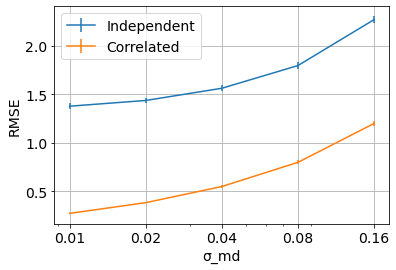
(a) RMSE as a function of $\sigma_{\text{md}}$.

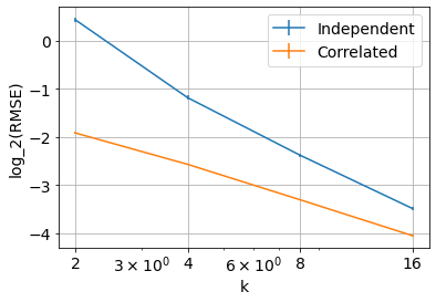
(b) RMSE as a function of $k$.

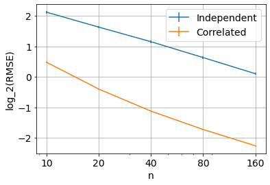
(c) RMSE as a function of $n$.

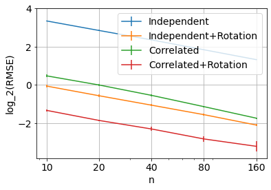
(d) RMSE with random rotation.

Figure 2: Comparison of compression algorithms on mean estimation task.

Table 1: Comparison of mean square error of compression algorithms on distributed mean estimation.

Algorithm	Synthetic	MNIST
Independent	$10.28(0.25)$	$0.466(0.014)$
Independent + Rotation	$3.29(0.19)$	$1.661(0.126)$
TernGrad ($\log_{2}(3)$ bits)	$2.64(0.01)$	$0.621(0.006)$
Structured DRIVE	$1.38(0.01)$	$2.165(0.006)$
Correlated	$1.40(0.05)$	$\mathbf{0.141(0.004)}$
Correlated + Rotation	$\mathbf{1.01(0.06)}$	$0.238(0.012)$

Table 2: Comparison of compression algorithms on a variety of tasks: distributed mean estimation, distributed $k$-means clustering, distributed power iteration, and federated averaging on the MNIST dataset. For all tasks, we set the number of quantization levels to two (one bit), except TernGrad which uses three quantization levels.

Algorithm	Dist. $k$-means	Dist. Power Iteration	FedAvg
	Objective	Error	Accuracy %
No quantization	$39.43(0.12)$	$0.008(0.000)$	$89.31(0.01)$
Independent	$42.98(0.23)$	$0.242(0.005)$	$87.38(0.30)$
Independent + Rotation	$68.85(2.81)$	$0.267(0.016)$	$89.11(0.06)$
TernGrad ($\log_{2}(3)$ bits)	$42.07(0.09)$	$0.100(0.001)$	$88.50(0.03)$
Structured DRIVE	$46.93(0.17)$	$0.370(0.001)$	$89.00(0.03)$
Correlated	$\mathbf{39.97(0.13)}$	$\mathbf{0.055(0.002)}$	$88.39(0.12)$
Correlated + Rotation	$42.21(0.17)$	$0.059(0.002)$	$\mathbf{89.20(0.04)}$

We demonstrate that the proposed algorithm outperforms existing baselines on several distributed tasks. Before we conduct a full comparison, we first empirically demonstrate that our correlated quantization algorithm is better than existing independent quantization schemes (Suresh et al., 2017; Alistarh et al., 2017). We implement all algorithms and experiments using the open-source JAX (Bradbury et al., 2018) and FedJAX (Ro et al., 2021) libraries . We simulated shared randomness by downstream communication from server to clients (Szlendak et al., 2021).

Correlated vs independent stochastic quantization. We first compare correlated and independent stochastic quantizations on a simple mean estimation task. Let $x_{1},x_{2},\ldots,x_{n}$ be $n$ i.i.d. samples over $\mathbb{R}^{1024}$, where coordinate $i$ is sampled independently according to $\mu(i)+U$, where $\mu(i)$ is a uniform random variable between $[0,1]$ and is fixed for all clients and $U$ is a independent random variable for each client in the range $[-4\sigma_{\text{md}},4\sigma_{\text{md}}]$. Note that this distribution has a mean deviation of $\sigma_{\text{md}}$. We first fix the number of clients $n$ to be $100$, $k=2$, and vary $\sigma_{\text{md}}$. We then fix $\sigma_{\text{md}}=0.01$, $n=100$ and vary $k$. Finally, we fix $\sigma_{\text{md}}=0.01$, $k=2$ and vary $n$. The results are given in Figures 2 $(a),(b),(c)$ respectively. The experiments are averaged over ten runs for statistical consistency. Observe that in all the experiments, correlated quantization outperforms independent stochastic quantization.

Effect of random rotation. We next demonstrate that the correlated quantization benefits from random rotation similar to independent quantization. Let $x_{1},x_{2},\ldots,x_{n}$ be $n$ i.i.d. samples over $\mathbb{R}^{1024}$, where coordinate $i$ is independently sampled according to $\mu(i)+U$, where $U$ is a independent random variable for each client in the range $[-4\sigma_{\text{md}},4\sigma_{\text{md}}]$. We let $\mu=(1.0,-1.0,0.0,\ldots,0.0)$, $k=2$, and $\sigma_{\text{md}}=0.01$. We compare the results as a function of $n$ in Figure 2 $(d)$. Observe that random rotation improves the performance of both correlated and independent quantization. Furthermore, rotated correlated quantization outperforms the remaining schemes.

In the following experiments, we compare our correlated quantization algorithm with several quantization baselines: Independent, Independent+Rotation (Suresh et al., 2017), TernGrad (Wen et al., 2017), and Structured DRIVE (Vargaftik et al., 2021b). Since the focus of the paper is quantization, we only compare lossy quantization schemes and do not evaluate the lossless compression schemes such as arithmetic coding or Huffman coding, which can be applied on any quantizer. We use 2-level quantization (one bit) for all the algorithms, except TernGrad which uses $3$ levels and hence requires $\log_{2}(3)$ bits per coordinate per client.

Distributed mean estimation. We next compare our proposed algorithm to existing baselines on a sparse mean estimation task. Let $x_{1},x_{2},\ldots,x_{n}$ be $n$ i.i.d. samples over $\mathbb{R}^{1024}$, where coordinate $i$ is sampled independently according to $\mu(i)+U$, where $\mu$ is a sparse vector with $1\%$ sparse entries and is fixed for all clients and $U$ is a independent random variable for each client in the range $[-4\sigma_{\text{md}},4\sigma_{\text{md}}]$. We also compare quantizers on the distributed mean estimation task for the MNIST ($d=784$) dataset distributed over $100$ clients. The results for both for $10$ repeated trials are in Table 1. Observe that correlated quantizers perform best.

Distributed k-means clustering. In the distributed Lloyd’s (k-means) algorithm, each client has access to a subset of data points and the goal of a server is to learn $k$-centers by repeatedly interacting with the clients. We employ quantizers to reduce the uplink communication cost from clients to server and use the MNIST ($d=784$) dataset and set both the number of centers and number of clients to 10. We split examples evenly amongst clients and use k-means++ to select the initial cluster centers. The results for $20$ communication rounds for $10$ repeated trials are in Table 2. Observe that correlated quantization performs the best.

Distributed power iteration. In distributed power iteration, each client has access to a subset of data and the goal of the server is to learn the top eigenvector. Similar to the previous distributed k-means clustering, in the quantized setting, we use quantization to reduce the communication cost from clients to server and use the MNIST ($d=784$) dataset distributed evenly over $100$ clients The results for $20$ communication rounds for $10$ repeated trials are in Table 2. Observe that correlated quantizers outperform all baselines.

Federated learning. We finally evaluate the effectiveness of the proposed algorithm in reducing the uplink communication costs in federated learning (McMahan et al., 2017). We use the image recognition task for the Federated MNIST dataset (Caldas et al., 2018a) provided by TensorFlow Federated (Bonawitz et al., 2019). This dataset consists of $341K$ training examples with $10$ label classes distributed across $3383$ clients. We use quantizers to reduce the uplink communication cost from clients to server and train a logistic regression model for $1000$ communication rounds of federated averaging for $5$ repeated trials. The results are in Table 2. Observe that correlated quantization with rotation achieves the highest test accuracy.

9 Conclusion

We proposed a new quantizer for distributed mean estimation and showed that the error guarantee depends on the deviation of data points instead of their absolute range. We further used this result to provide fast convergence rates for distributed optimization under communication constraints. Experimental results show that our proposed algorithm outperforms existing compression protocols on several tasks. We also proved the optimality of the proposed approach under mild assumptions in one dimension. Extending the lower bounds to high dimensions remains an interesting open question.

Appendix A Proof of Theorem 2

See 2

Proof.

We first show the result when $l=0$ and $r=1$, one can obtain the final result by rescaling the quantizer operation

$$(l-u)\cdot Q_{i}\left(\frac{x_{i}}{u-l}\right).$$

Hence in the following, without loss of generality, let $l=0,r=1$. We first show that $Q$ is an unbiased equantizer

$$\mathbb{E}[Q_{i}(x_{i})] =\mathbb{E}[1_{\frac{\pi_{i}}{n}+\gamma_{i}<x_{i}}].$$

Observe that $\frac{\pi_{i}}{n}+\gamma_{i}$ is a uniform random variable between $[0,1)$. Hence,

$$\mathbb{E}[Q_{i}(x_{i})] =\mathbb{E}[1_{\frac{\pi_{i}}{n}+\gamma_{i}<x_{i}}]=\text{Pr}\left(\frac{\pi_{i}}{n}+\gamma_{i}<x_{i}\right)=x_{i}.$$

We now bound its variance. To this end let

$$y_{i}=\frac{\lfloor nx_{i}\rfloor}{n}.$$

We can rewrite the difference between estimate and the true sum as

$$\sum^{n}_{i=1}x_{i}-\sum^{n}_{i=1}Q_{i}(x_{i}) =\sum^{n}_{i=1}x_{i}-\sum^{n}_{i=1}y_{i}+\sum^{n}_{i=1}y_{i}-\sum^{n}_{i=1}Q_{i}(y_{i})+\sum^{n}_{i=1}Q_{i}(y_{i})-\sum^{n}_{i=1}Q_{i}(x_{i}).$$

Since $(a+b+c)^{2}\leq 3a^{2}+3b^{2}+3c^{2}$,

$$\mathbb{E}\left[\left(\sum^{n}_{i=1}x_{i}-\sum^{n}_{i=1}Q_{i}(x_{i})\right)^{2}\right]= 3\mathbb{E}\left[\left(\sum^{n}_{i=1}x_{i}-\sum^{n}_{i=1}y_{i}\right)^{2}\right]$$

$$+3\mathbb{E}\left[\left(\sum^{n}_{i=1}y_{i}-\sum^{n}_{i=1}Q_{i}(y_{i})\right)^{2}\right]+3\mathbb{E}\left[\left(\sum^{n}_{i=1}Q_{i}(y_{i})-\sum^{n}_{i=1}Q_{i}(x_{i})\right)^{2}\right].$$

We now bound each of the three terms in the above summation.

First term: Observe that for all $i$

$$|x_{i}-y_{i}|\leq\frac{1}{n}.$$

Hence,

$$\left\lvert\sum^{n}_{i=1}x_{i}-\sum^{n}_{i=1}y_{i}\right\rvert\leq\sum^{n}_{i=1}|x_{i}-y_{i}|\leq n\cdot\frac{1}{n}=1.$$

Therefore,

$$\mathbb{E}\left[\left(\sum^{n}_{i=1}x_{i}-\sum^{n}_{i=1}y_{i}\right)^{2}\right]\leq 1.$$

Second term: To bound the second term,

$$\mathbb{E}\left[\left(\sum^{n}_{i=1}y_{i}-\sum^{n}_{i=1}Q_{i}(y_{i})\right)^{2}\right] =\sum^{n}_{i=1}\mathbb{E}\left[\left(y_{i}-Q_{i}(y_{i})\right)^{2}\right]+\sum^{n}_{i=1}\sum_{j\neq i}\mathbb{E}\left[\left(y_{i}-Q_{i}(y_{i})\right)\left(y_{j}-Q_{j}(y_{j})\right)\right]$$

$$=\sum^{n}_{i=1}y_{i}(1-y_{i})+\sum^{n}_{i=1}\sum_{j\neq i}\mathbb{E}\left[\left(y_{i}-Q_{i}(y_{i})\right)\left(y_{j}-Q_{j}(y_{j})\right)\right]$$

$$=\sum^{n}_{i=1}y_{i}(1-y_{i})+\sum^{n}_{i=1}\sum_{j\neq i}\left(\mathbb{E}\left[Q_{i}(y_{i})Q_{j}(y_{j})\right]-y_{i}y_{j}\right),$$

where the second equality uses the fact that $1_{\frac{\pi_{i}}{n}+\gamma_{i}<y_{i}}$ is a Bernoulli random variable with parameter $y_{i}$. We now bound $\mathbb{E}\left[Q_{i}(y_{i})Q_{j}(y_{j})\right]-y_{i}y_{j}$ for $i\neq j$. observe that

$$Q_{i}(y_{i})=1_{\frac{\pi_{i}}{n}+\gamma_{i}<y_{i}}.$$

However, since $y_{i}$ is an integral multiple of $1/n$, and $\gamma_{i}\in[0,1/n)$, $\frac{\pi_{i}}{n}+\gamma_{i}<y_{i}$ if and only if $\frac{\pi_{i}}{n}<y_{i}$. Hence,

$$Q_{i}(y_{i})=1_{\frac{\pi_{i}}{n}<y_{i}}.$$

Hence,

$$\mathbb{E}\left[Q_{i}(y_{i})Q_{j}(y_{j})\right]=\mathbb{E}\left[1_{\frac{\pi_{i}}{n}<y_{i}}1_{\frac{\pi_{j}}{n}<y_{j}}\right]=\text{Pr}\left(\pi_{i}<ny_{i}\cap\pi_{j}<ny_{j}\right).$$

Since $\pi$ is a random permutation,

$$\text{Pr}\left(\pi_{i}<ny_{i}\cap\pi_{j}<ny_{j}\right) =\frac{1}{n(n-1)}\min(ny_{i},ny_{j})\cdot\left(\max(ny_{i},ny_{j})-1\right)$$

$$=\frac{ny_{i}y_{j}}{(n-1)}-\frac{\min(y_{i},y_{j})}{(n-1)}$$

$$=\frac{ny_{i}y_{j}}{(n-1)}-\frac{y_{i}+y_{j}}{2(n-1)}+\frac{|y_{i}-y_{j}|}{2(n-1)}.$$

Hence,

$$\sum^{n}_{i=1}\sum_{j\neq i}\left(\mathbb{E}\left[Q_{i}(y_{i})Q_{j}(y_{j})\right]-y_{i}y_{j}\right) =\sum^{n}_{i=1}\sum_{j\neq i}\left(\frac{ny_{i}y_{j}}{(n-1)}-\frac{y_{i}+y_{j}}{2(n-1)}+\frac{|y_{i}-y_{j}|}{2(n-1)}-y_{i}y_{j}\right)$$

$$=\frac{1}{n-1}\sum^{n}_{i=1}\sum_{j\neq i}\left(y_{i}y_{j}-\frac{y_{i}+y_{j}}{2}+\frac{|y_{i}-y_{j}|}{2}\right)$$

$$=\frac{1}{n-1}\left(\Bigl{(}\sum^{n}_{i=1}y_{i}\Bigr{)}^{2}-\sum^{n}_{i=1}y^{2}_{i}-(n-1)\sum^{n}_{i=1}y_{i}+\sum^{n}_{i=1}\sum_{j\neq i}\frac{|y_{i}-y_{j}|}{2}\right)$$

$$=\sum^{n}_{i=1}\sum_{j\neq i}\frac{|y_{i}-y_{j}|}{2(n-1)}+\frac{1}{n-1}\left(\Bigl{(}\sum^{n}_{i=1}y_{i}\Bigr{)}^{2}-\sum^{n}_{i=1}y^{2}_{i}\right)-\sum_{i}y_{i}$$

$$\leq\sum^{n}_{i=1}\sum_{j\neq i}\frac{|y_{i}-y_{j}|}{2(n-1)}+\frac{1}{n}\left(\Bigl{(}\sum^{n}_{i=1}y_{i}\Bigr{)}^{2}\right)-\sum^{n}_{i=1}y_{i}$$

Hence,

$$\mathbb{E}\left[\left(\sum^{n}_{i=1}y_{i}-\sum^{n}_{i=1}Q_{i}(y_{i})\right)^{2}\right] =\sum^{n}_{i=1}y_{i}(1-y_{i})+\sum^{n}_{i=1}\sum_{j\neq i}\left(\mathbb{E}\left[Q_{i}(y_{i})Q_{j}(y_{j})\right]-y_{i}y_{j}\right)$$

$$\leq\sum^{n}_{i=1}y_{i}(1-y_{i}){\color[rgb]{0,0,0}+}\sum^{n}_{i=1}\sum_{j\neq i}\frac{|y_{i}-y_{j}|}{2(n-1)}+\frac{1}{n}\left((\sum_{i}y_{i})^{2}\right)-\sum_{i}y_{i}$$

$$=\sum^{n}_{i=1}\sum_{j\neq i}\frac{|y_{i}-y_{j}|}{2(n-1)}+\frac{1}{n}\left(\Bigl{(}\sum^{n}_{i=1}y_{i}\Bigr{)}^{2}\right)-\sum^{n}_{i=1}y^{2}_{i}$$

$$\leq\sum^{n}_{i=1}\sum_{j\neq i}\frac{|y_{i}-y_{j}|}{2(n-1)}$$

$$\leq\sum^{n}_{i=1}\sum_{j\neq i}\frac{|x_{i}-x_{j}|}{2(n-1)}+\sum^{n}_{i=1}\sum_{j\neq i}\frac{1}{2n(n-1)}$$

$$\leq\sum^{n}_{i=1}\sum_{j\neq i}\frac{|x_{i}-x_{j}|}{2(n-1)}+1.$$

Third term: Observe that

$$Q_{i}(y_{i})-Q_{i}(x_{i})=1_{\frac{\pi_{i}}{n}+\gamma_{i}<y_{i}}-1_{\frac{\pi_{i}}{n}+\gamma_{i}<x_{i}}.$$

Since $x_{i}\geq y_{i}$, $1_{\frac{\pi_{i}}{n}+\gamma_{i}<y_{i}}$ implies $1_{\frac{\pi_{i}}{n}+\gamma_{i}<x_{i}}$. Hence $Q_{i}(y_{i})-Q_{i}(x_{i})$ takes at most two values $0,-1$. Therefore,

$$Q_{i}(y_{i})-Q_{i}(x_{i})=-1_{y_{i}\leq\frac{\pi_{i}}{n}+\gamma_{i}<x_{i}}.$$

Therefore,

$$\mathbb{E}\left[\left(\sum^{n}_{i=1}Q_{i}(y_{i})-\sum^{n}_{i=1}Q_{i}(x_{i})\right)^{2}\right]$$

$$=\sum^{n}_{i=1}\mathbb{E}\left[\left(Q_{i}(y_{i})-Q_{i}(x_{i})\right)^{2}\right]+\sum^{n}_{i=1}\sum_{j\neq i}\mathbb{E}\left[\left(Q_{i}(y_{i})-{\color[rgb]{0,0,0}Q_{i}(x_{i})}\right)\left(Q_{j}(y_{j})-Q_{j}(x_{j})\right)\right]$$

$$=\sum^{n}_{i=1}\mathbb{E}\left[1_{y_{i}\leq\frac{\pi_{i}}{n}+\gamma_{i}<x_{i}}\right]+\sum^{n}_{i=1}\sum_{j\neq i}\mathbb{E}\left[1_{y_{i}\leq\frac{\pi_{i}}{n}+\gamma_{i}<x_{i}}1_{y_{j}\leq\frac{\pi_{j}}{n}+\gamma_{j}<x_{j}}\right]$$

$$=\sum^{n}_{i=1}\mathbb{E}\left[1_{y_{i}\leq\frac{\pi_{i}}{n}+\gamma_{i}<y_{i}+1}\right]+\sum^{n}_{i=1}\sum_{j\neq i}\mathbb{E}\left[1_{y_{i}\leq\frac{\pi_{i}}{n}+\gamma_{i}<y_{i}+1}1_{y_{j}\leq\frac{\pi_{j}}{n}+\gamma_{j}<y_{j}+1}\right]$$

$$=\sum^{n}_{i=1}\mathbb{E}\left[1_{y_{i}\leq\frac{\pi_{i}}{n}<y_{i}+1}\right]+\sum^{n}_{i=1}\sum_{j\neq i}\mathbb{E}\left[1_{y_{i}\leq\frac{\pi_{i}}{n}<y_{i}+1}1_{y_{j}\leq\frac{\pi_{j}}{n}<y_{j}+1}\right]$$

$$\leq\sum^{n}_{i=1}\frac{1}{n}+\sum^{n}_{i=1}\sum_{j\neq i}\frac{1}{n(n-1)}$$

$$=2.$$

Combining the analysis of the above three terms we get

$$\mathbb{E}\left[\left(\sum^{n}_{i=1}x_{i}-\sum^{n}_{i=1}Q_{i}(x_{i})\right)^{2}\right]\leq\sum^{n}_{i=1}\sum_{j\neq i}\frac{3|x_{i}-x_{j}|}{2(n-1)}+12.$$

Hence,

$$\mathcal{E}(Q^{n},x^{n}) \leq\sum^{n}_{i=1}\sum_{j\neq i}\frac{3|x_{i}-x_{j}|}{2n^{2}(n-1)}+\frac{12}{n^{2}}$$

$$\leq\frac{3}{2n}\cdot\frac{1}{n(n-1)}\sum^{n}_{i=1}\sum_{j\neq i}|x_{i}-x_{j}|+\frac{12}{n^{2}}.$$

The lemma follows by observing that

$$\frac{1}{n(n-1)}\sum^{n}_{i=1}\sum_{j\neq i}|x_{i}-x_{j}|\leq 2\sigma_{\text{md}}.$$

∎

Appendix B Proof of Theorem 3

See 3

Proof.

Similar to the proof of Theorem 2, without loss of generality, we let $l=0,r=1$. One can obtain the final result by rescaling the quantizer via

$$(l-u)\cdot Q_{i}\left(\frac{x_{i}}{u-l}\right).$$

The proof of unbiasedness is similar to the proof of Theorem 2 and is omitted. We now bound its variance. Let $z_{i}=\frac{x_{i}-c^{\prime}_{i}}{\beta}$. We wish to bound

$$\sum^{n}_{i=1}x_{i}-\sum^{n}_{i=1}Q_{i}(x_{i})=\beta\left(\sum^{n}_{i=1}z_{i}-\sum^{n}_{i=1}Q_{i}\left(z_{i}\right)\right).$$

Similar to the proof of Theorem 2, it can be shown that

$$\mathbb{E}\left[\left(\sum^{n}_{i=1}z_{i}-\sum^{n}_{i=1}Q_{i}(z_{i})\right)^{2}|c^{\prime}\right]\leq\sum^{n}_{i=1}\sum_{j\neq i}\frac{3|z_{i}-z_{j}|}{2(n-1)}+12.$$

Hence,

$$\mathbb{E}\left[\left(\sum^{n}_{i=1}x_{i}-\sum^{n}_{i=1}Q_{i}(x_{i})\right)^{2}|c^{\prime}\right] \leq\beta^{2}\sum^{n}_{i=1}\sum_{j\neq i}\frac{3|z_{i}-z_{j}|}{2(n-1)}+12\beta^{2}.$$

If $|x_{i}-x_{j}|\geq\beta$, then

$$|z_{i}-z_{j}|\leq 1.$$

If $|x_{i}-x_{j}|\leq\beta$, then

$$\mathbb{E}[|z_{i}-z_{j}|] =\text{Pr}(c^{\prime}_{i}=c^{\prime}_{j})\mathbb{E}[|z_{i}-z_{j}|1_{c^{\prime}_{i}=c^{\prime}_{j}}]+\text{Pr}(c^{\prime}_{i}\neq c^{\prime}_{j})\mathbb{E}[|z_{i}-z_{j}|1_{c^{\prime}_{i}\neq c^{\prime}_{j}}]$$

$$\leq\text{Pr}(c^{\prime}_{i}=c^{\prime}_{j})\mathbb{E}[|z_{i}-z_{j}|1_{c^{\prime}_{i}=c^{\prime}_{j}}]+\text{Pr}(c^{\prime}_{i}\neq c^{\prime}_{j})$$

$$\leq\text{Pr}(c^{\prime}_{i}=c^{\prime}_{j})\frac{|x_{i}-x_{j}|}{\beta}+\text{Pr}(c^{\prime}_{i}\neq c^{\prime}_{j})$$

$$\leq\frac{|x_{i}-x_{j}|}{\beta}+\text{Pr}(c^{\prime}_{i}\neq c^{\prime}_{j})$$

$$\leq\frac{|x_{i}-x_{j}|}{\beta}+\frac{|x_{i}-x_{j}|}{\beta}\ =2\frac{|x_{i}-x_{j}|}{\beta}.$$

Hence,

$$\mathbb{E}[|z_{i}-z_{j}|]\leq 2\left(\min\left(\frac{|x_{i}-x_{j}|}{\beta},1\right)\right).$$

Therefore,

$$\mathbb{E}\left[\left(\sum^{n}_{i=1}x_{i}-\sum^{n}_{i=1}Q_{i}(x_{i})\right)^{2}\right] \leq\sum^{n}_{i=1}\sum_{j\neq i}\beta\frac{3\min\left(|x_{i}-x_{j}|,\beta\right)}{(n-1)}+12\beta^{2}$$

$$\leq 3\min\left(\sum^{n}_{i=1}\sum_{j\neq i}\frac{\beta|x_{i}-x_{j}|}{(n-1)},n\beta^{2}\right)+12\beta^{2}$$

$$\leq 3\min\left(2n\beta\sigma_{\text{md}},n\beta^{2}\right)+12\beta^{2}.$$

$$\mathcal{E}(Q^{n},x^{n}) \leq\frac{3}{n}\cdot\min\left(2\beta\sigma_{\text{md}},\beta^{2}\right)+\frac{12\beta^{2}}{n^{2}}.$$

Combining with the fact that $\beta\leq 2/k$ yields the result. ∎

Appendix C Proof of Corollary 2

See 2

Proof.

The communication cost follows by observing that we are communication $k$ level of quantization for each coordinate. We first bound the bias. Observe that

$$\|{\bar{x}}-\mathbb{E}[\hat{x}]\|_{2}^{2} \leq\frac{1}{n}\sum^{n}_{i=1}\left\lVert x_{i}-\frac{R\sqrt{8\log(dn)}}{\sqrt{d}}\mathbb{E}[W^{-1}\cdot z_{i}]\right\rVert_{2}^{2}$$

$${\color[rgb]{0,0,0}=\frac{1}{n}\sum^{n}_{i=1}\left\lVert\mathbb{E}\left[W^{-1}\cdot\left(W\cdot x_{i}-\frac{R\sqrt{8\log(dn)}}{\sqrt{d}}z_{i}\right)\right]\right\rVert_{2}^{2}}$$

$${\color[rgb]{0,0,0}\leq\frac{1}{n}\sum^{n}_{i=1}\mathbb{E}\left[\left\lVert W^{-1}\cdot\left(W\cdot x_{i}-\frac{R\sqrt{8\log(dn)}}{\sqrt{d}}z_{i}\right)\right\rVert_{2}^{2}\right]}$$

$${\color[rgb]{0,0,0}\leq\frac{1}{n}\sum^{n}_{i=1}\mathbb{E}\left[\left\lVert W\cdot x_{i}-\frac{R\sqrt{8\log(dn)}}{\sqrt{d}}z_{i}\right\rVert_{2}^{2}\right]}$$

$$\leq\frac{1}{n}\sum^{n}_{i=1}18R^{2}\log(dn)\Pr\left(\frac{\sqrt{d}}{R\sqrt{8\log(dn)}}W\cdot x_{i}\neq z_{i}\right),$$

where the last inequality follows from that when $\frac{\sqrt{d}}{R\sqrt{8\log(dn)}}W\cdot x_{i}\neq z_{i}$, the error is at most

$$\left\lVert W\cdot x_{i}-\frac{R\sqrt{8\log(dn)}}{\sqrt{d}}z_{i}\right\rVert_{2}^{2}\leq 18R^{2}\log(dn).$$

Next we bound $\Pr\left(\frac{\sqrt{d}}{R\sqrt{8\log(dn)}}W\cdot x_{i}\neq z_{i}\right)$ for each $x_{i}$. For any $x$ with $\lVert x\rVert\leq R$,

$$\Pr\left(\frac{\sqrt{d}}{R\sqrt{8\log(dn)}}W\cdot x\neq z\right) \leq\sum_{j=1}^{d}\Pr\left(\frac{\sqrt{d}}{R\sqrt{8\log(dn)}}[Wx](j)\neq z(j)\right)$$

$$\leq\sum_{j=1}^{d}\Pr\left([Wx](j)\geq\frac{\sqrt{8\log(dn))}}{\sqrt{d}}\|x\|_{2}\right)$$

$$\stackrel{{\scriptstyle(b)}}{{\leq}}de^{-4\log(dn)},$$

where $(b)$ follows from McDiamid’s inequality. Hence,

$$\|{\bar{x}}-\mathbb{E}[\hat{x}]\|_{2}^{2}\leq\frac{18R^{2}\log(dn)}{d^{3}n^{4}}.$$

To bound the mean squared error, observe that

$$\mathbb{E}\|{\bar{x}}-\hat{x}]\|^{2}_{2} =\mathbb{E}\|{\bar{x}}-\mathbb{E}[\hat{x}]]\|^{2}_{2}+\mathbb{E}\|\hat{x}-\mathbb{E}[\hat{x}]]\|^{2}_{2}$$

$$=\|{\bar{x}}-\mathbb{E}[\hat{x}]]\|^{2}_{2}+\mathbb{E}\|\hat{x}-\mathbb{E}[\hat{x}]]\|^{2}_{2}$$

$$\leq\|{\bar{x}}-\mathbb{E}[\hat{x}]]\|^{2}_{2}+\mathbb{E}\|W\hat{x}-\mathbb{E}[W\hat{x}]]\|^{2}_{2}$$

$$\leq\frac{18R^{2}\log(dn)}{d^{3}n^{4}}+\mathbb{E}\|W\hat{x}-\mathbb{E}[W\hat{x}]]\|^{2}_{2}.$$

For $j\in[d]$, let $y^{n}(j)=(y_{1}(j),\ldots,y_{n}(j))$ denote the scalar dataset which only consists of the $j$th coordinate of $y^{n}$. Define $\sigma_{\text{md}}(y^{n}(j))$ to be the corresponding empirical mean absolute deviation.

$$\mathbb{E}\|W\hat{x}-\mathbb{E}[W\hat{x}]]\|^{2}_{2} =\frac{R^{2}(8\log(dn))}{d}\mathbb{E}\|z-\mathbb{E}[z]]\|^{2}_{2}$$

$$\leq\frac{R^{2}(8\log(dn))}{d}\left(\frac{12}{n}\cdot\sum^{d}_{j=1}\min\left(\frac{\mathbb{E}[\sigma_{\text{md}}(y^{n\prime}(j))]}{k},\frac{1}{k^{2}}\right)+\frac{48d}{n^{2}k^{2}}\right)$$

$$\leq\frac{R^{2}(8\log(dn))}{d}\left(\frac{12}{n}\cdot\sum^{d}_{j=1}\min\left(\frac{2\mathbb{E}[\sigma_{\text{md}}(y^{n}(j))]}{k},\frac{1}{k^{2}}\right)+\frac{48d}{n^{2}k^{2}}\right)$$

$$\leq\frac{R^{2}(8\log(dn))}{d}\left(\frac{12}{n}\cdot\min\left(\frac{2\sum^{d}_{j=1}\mathbb{E}[\sigma_{\text{md}}(y^{n}(j))]}{k},\frac{d}{k^{2}}\right)+\frac{48d}{n^{2}k^{2}}\right)$$

$$\leq\frac{R^{2}(8\log(dn))}{d}\left(\frac{12}{n}\cdot\min\left(\frac{2\sqrt{d}\cdot\mathbb{E}[\sigma^{d}_{\text{md}}(y^{n})]}{k},\frac{d}{k^{2}}\right)+\frac{48d}{n^{2}k^{2}}\right)$$

$$\stackrel{{\scriptstyle(c)}}{{\leq}}(8\log(dn))\left(\frac{12}{n}\cdot\min\left(\frac{2R\sigma^{d}_{\text{md}}(x^{n})}{k},\frac{R^{2}}{k^{2}}\right)+\frac{48R^{2}}{n^{2}k^{2}}\right)$$

$$\leq\frac{192\log(dn)}{n}\cdot\min\left(\frac{R\sigma^{d}_{\text{md}}(x^{n})}{k},\frac{R^{2}}{k^{2}}\right)+\frac{392R^{2}\log(dn)}{n^{2}k^{2}},$$

where $(c)$ uses the fact that $\sigma^{d}_{\text{md}}(y^{n})=\frac{\sqrt{d}}{R\sqrt{8\log(dn)}}\sigma^{d}_{\text{md}}(x^{n})$ since $y^{n}$ is a scaled rotated version of $x^{n}$. Combining the above two results yields the result. ∎

Appendix D Proof of Lower bounds (Theorem 4 and Theorem 5)

A general $k$-level randomized quantizer $Q^{n}$ can be viewed as a distribution over $\mathcal{Q}_{\text{det}}$, which contains all deterministic mappings from $[l,r]^{n}$ to $[k]^{n}$. Let $\mathcal{Q}_{\text{rand}}$ be all randomized mappings from $[l,r]^{n}$ to $[k]^{n}$. To establish a lower bound for general quantizer, we use Yao’s minimax principle to reduce it to a lower bound over $\mathcal{Q}_{\text{det}}$,

$$\min_{Q^{n}{\color[rgb]{0,0,0}\in\mathcal{Q}_{\text{rand}}}}\max_{x^{n}}\mathcal{E}(Q^{n},x^{n})\geq\max_{P}\min_{Q^{n}\in\mathcal{Q}_{\text{det}}}\mathbb{E}_{X^{n}\sim P}\left[\mathcal{E}(Q^{n},X^{n})\right]=\max_{P}\min_{Q^{n}\in\mathcal{Q}_{\text{det}}}\mathbb{E}_{X^{n}\sim P}\left[\left(\hat{x}(Q^{n}(X^{n}))-\frac{1}{n}\sum_{i=1}^{n}X_{i}\right)^{2}\right].$$ (5)

In the rest of the proof, we focus on deterministic $Q_{i}$’s and bound (5). Without loss of generality we assume $l=0$. We first prove the following general lemma, which will be useful to prove both lower bounds.

Lemma 1.

Suppose under distribution $P$ over $[0,r]^{n}$, $X_{i}$’s are sampled i.i.d from $p$ over $[0,r]$, for any deterministic quantizer $Q^{n}$, we have

$$\mathbb{E}_{X^{n}\sim P}\left[\left(\hat{x}(Q^{n}(X^{n}))-\frac{1}{n}\sum^{n}_{i=1}X_{i}\right)^{2}\right]\geq\frac{1}{n^{2}}\sum_{i=1}^{n}\mathbb{E}_{X_{i}\sim p}\left[\left(X_{i}-\mathbb{E}\left[X_{i}\mid Q_{i}(X_{i})\right]\right)^{2}\right].$$

Proof.

Since conditional expectation minimizes the mean squared error over all functions of $\hat{x}(Q^{n}(X^{n}))$, we have

$$\mathbb{E}_{X^{n}\sim P}\left[\left(\hat{x}(Q^{n}(X^{n}))-\frac{1}{n}\sum^{n}_{i=1}X_{i}\right)^{2}\right]\geq\mathbb{E}_{X^{n}\sim P}\left[\left(\mathbb{E}\left[\frac{1}{n}\sum_{i=1}^{n}X_{i}\mid Q^{n}(X^{n})\right]-\frac{1}{n}\sum^{n}_{i=1}X_{i}\right)^{2}\right].$$

Note that since $X_{i}$’s are independent and $Q^{n}$ is deterministic, we have all $Q_{i}(X_{i})$ are independent. Moreover, this implies $Q_{j}(X_{j})$ is independent of $X_{i}$ for $i\neq j$. Hence

$$\mathbb{E}\left[\frac{1}{n}\sum_{i=1}^{n}X_{i}\mid Q^{n}(X^{n})\right]=\frac{1}{n}\sum_{i=1}^{n}\mathbb{E}\left[X_{i}\mid Q_{i}(X_{i})\right].$$

Combining these, we get

$$\mathbb{E}_{X^{n}\sim P}\left[\left(\hat{x}(Q^{n}(X^{n}))-\frac{1}{n}\sum^{n}_{i=1}X_{i}\right)^{2}\right]\geq\frac{1}{n^{2}}\sum_{i=1}^{n}\mathbb{E}_{X_{i}\sim p}\left[\left(X_{i}-\mathbb{E}\left[X_{i}\mid Q_{i}(X_{i})\right]\right)^{2}\right].$$

∎

Next we use Lemma 1 to prove Theorems 4 and 5.

See 4

Proof.

Consider the following distribution $p$ over $[0,r]$ where

$$p\left(x\right)=\begin{cases}\frac{\sigma_{\text{md}}}{2r}&\text{ if }x=0,\\ \frac{\sigma_{\text{md}}}{2r}&\text{ if }x=r,\\ 1-\frac{\sigma_{\text{md}}}{r}&\text{ if }x=\frac{r}{2},\\ 0&\text{ otherwise.}\end{cases}$$

We first show that if $P$ is the distribution where $X^{n}$ is sampled i.i.d from $p$,

$$\mathbb{E}_{X^{n}\sim P}\left[\left(\hat{x}(Q^{n}(X^{n}))-\frac{1}{n}\sum_{i=1}^{n}X_{i}\right)^{2}\right]\geq\frac{\sigma_{\text{md}}\cdot r}{32n}.$$

Applying Lemma 1, it is enough to show that for any $Q_{i}$, we have

$$\mathbb{E}_{X_{i}\sim p}\left[\left(X_{i}-\mathbb{E}\left[X_{i}\mid Q_{i}(X_{i})\right]\right)^{2}\right]\geq\frac{\sigma_{\text{md}}\cdot r}{32}.$$

Since $Q_{i}$ only outputs 1 bit, there must exist two numbers in $\{0,r/2,r\}$ such that they are mapped to the same output. If $\{0,r/2\}$ are mapped to the same output, we have $\mathbb{E}\left[X_{i}\mid Q_{i}(X_{i})=Q_{i}(0)\right]=\left(\frac{1-\frac{\sigma_{\text{md}}}{r}}{1-\frac{\sigma_{\text{md}}}{2r}}\right)\frac{r}{2}\geq\frac{r}{4}$. Hence,

$$\mathbb{E}_{X_{i}\sim p}\left[\left(X_{i}-\mathbb{E}\left[X_{i}\mid Q_{i}(X_{i})\right]\right)^{2}\right] \geq\text{Pr}\left(X_{i}=0\right)\cdot\left(\mathbb{E}\left[X_{i}\mid Q_{i}(X_{i})=Q_{i}(0)\right]\right)^{2}$$

$$\geq\frac{\sigma_{\text{md}}}{2r}\left(\frac{r}{4}\right)^{2}=\frac{\sigma_{\text{md}}\cdot r}{32}.$$

The same result holds when $\{r/2,r\}$ are mapped to the same output. When $\{0,r\}$ are mapped to the same output, we have

$$\mathbb{E}_{X_{i}\sim p}\left[\left(X_{i}-\mathbb{E}\left[X_{i}\mid Q_{i}(X_{i})\right]\right)^{2}\right] \geq\text{Pr}\left(X_{i}=0\text{ or }r\right)\cdot\mathbb{E}_{X_{i}\mid Q_{i}(X_{i})=Q_{i}(0)}\left[\left(X_{i}-\mathbb{E}\left[X_{i}\mid Q_{i}(X_{i})=Q_{i}(0)\right]\right)^{2}\right]$$

$$\geq\frac{\sigma_{\text{md}}}{r}\times\left(\frac{r}{2}\right)^{2}=\frac{\sigma_{\text{md}}\cdot r}{4}.$$

The last step is to check the mean absolute deviation. The proof is not complete yet since not all samples $X^{n}$ from the distribution $P$ has mean deviation $O(\sigma_{\text{md}})$. Next we construct a distribution $P^{\prime}$ where all $X^{n}\sim P^{\prime}$ has mean deviation $O(\sigma_{\text{md}})$ while the quantity in (5) is still lower bounded by $\Omega(\sigma_{\text{md}}\cdot r)$. We start by noting that the mean deviation can be upper bounded as

$$\frac{1}{n}\sum_{i=1}^{n}|X_{i}-\frac{1}{n}\sum_{i=1}^{n}X_{i}|\leq\frac{1}{n^{2}}\sum_{i,j\in[n]}|X_{i}-X_{j}|=\frac{1}{n^{2}}\frac{r}{2}\left(N_{0}N_{\frac{r}{2}}+N_{r}N_{\frac{r}{2}}+2N_{0}N_{r}\right),$$

where $N_{0},N_{\frac{r}{2}},N_{r}$ denote the number of appearances of $0,\frac{r}{2}$ and $r$ respectively. When $N_{0}+N_{r}<\frac{4n\sigma_{\text{md}}}{r}$, we have

$$\frac{1}{n^{2}}\frac{r}{2}\left(N_{0}N_{\frac{r}{2}}+N_{r}N_{\frac{r}{2}}+2N_{0}N_{r}\right)\leq\frac{1}{n^{2}}\frac{r}{2}\left(n\cdot\frac{4n\sigma_{\text{md}}}{r}+\left(\frac{2n\sigma_{\text{md}}}{r}\right)^{2}\right)\leq 4\sigma_{\text{md}}.$$

Since $N_{0}+N_{r}$ is a binomial random variable with $n$ trials and success probability $\frac{\sigma_{\text{md}}}{r}$, by Chernoff bound, we have

$$\text{Pr}\left(N_{0}+N_{r}\geq\frac{4n\sigma_{\text{md}}}{r}\right)\leq\exp\left(-\frac{2n\sigma_{\text{md}}}{r}\right)\leq\left(\frac{\sigma_{\text{md}}}{r}\right)^{16}.$$

Let $P^{\prime}$ be the distribution of $X^{n}$ conditioned on the event that $N_{0}+N_{r}<\frac{4n\sigma_{\text{md}}}{r}$, we have

$$\mathbb{E}_{X^{n}\sim P}\left[\left(\hat{x}(Q^{n}(X^{n}))-\frac{1}{n}\sum_{i=1}^{n}X_{i}\right)^{2}\right] \leq\text{Pr}\left(N_{0}+N_{r}<\frac{4n\sigma_{\text{md}}}{r}\right)\mathbb{E}_{X^{n}\sim P^{\prime}}\left[\left(\hat{x}(Q^{n}(X^{n}))-\frac{1}{n}\sum_{i=1}^{n}X_{i}\right)^{2}\right]$$

$$\;\;\;\;\;\;\;\;\;\;\;\;\;\;\;\;\;\;+r^{2}\text{Pr}\left(N_{0}+N_{r}\geq\frac{4n\sigma_{\text{md}}}{r}\right),$$

since when $N_{0}+N_{r}\geq\frac{4n\sigma_{\text{md}}}{r}$, the error is bounded by at most $r^{2}$ since the the optimal mean lies in $[0,r]$. Hence we have

$$\mathbb{E}_{X^{n}\sim P^{\prime}}\left[\left(\hat{x}(Q^{n}(X^{n}))-\frac{1}{n}\sum_{i=1}^{n}X_{i}\right)^{2}\right] \geq\mathbb{E}_{X^{n}\sim P}\left[\left(\hat{x}(Q^{n}(X^{n}))-\frac{1}{n}\sum_{i=1}^{n}X_{i}\right)^{2}\right]-r^{2}\text{Pr}\left(N_{0}+N_{r}\geq\frac{4n\sigma_{\text{md}}}{r}\right)$$

$$\geq\frac{\sigma_{\text{md}}\cdot r}{64n}.$$

This completes the proof using (5).

∎

See 5

Proof.

We show that

$$\mathcal{E}(Q^{n},x^{n})\geq\max\left(\frac{\sigma_{\text{md}}(r-l)}{32nk}+\frac{(r-l)^{2}}{64n^{2}k^{2}}\right).$$

The lemma follows by the fact that maximum is lower bounded by the average. Note that here it would be enough to prove the two terms in the above lower bound separately. Assuming $l=0$, for the $\frac{\sigma_{\text{md}}\cdot r}{32nk}$ term, we assume $n=\Omega(\frac{r}{k\sigma_{\text{md}}})$ since otherwise the second term dominates. We consider $2k$ distributions $p_{1},p_{2},\ldots,p_{2k}$ where for $j\in\{1,\ldots,2k\}$,

$$p_{j}\left(x\right)=\begin{cases}\frac{k\sigma_{\text{md}}}{r}&\text{ if }x=(j-1)\cdot\frac{r}{2k},\\ 1-\frac{k\sigma_{\text{md}}}{r}&\text{ if }x=j\cdot\frac{r}{2k},\\ 0&\text{ otherwise.}\end{cases}$$

Then we define $\bar{P}$ over $[0,r]^{n}$ as a uniform mixture of $b$ distributions,

$$\bar{P}=\frac{1}{2k}\sum_{j=1}^{2k}P_{j}.$$

where under $P_{j}$, $X_{i}$’s are $n$ i.i.d samples from $p_{j}$. Then we have for any deterministic quantization scheme $Q^{n}$,

$$\mathbb{E}_{X^{n}\sim\bar{P}}\left[\left(\hat{x}(Q^{n}(X^{n}))-\frac{1}{n}\sum_{i=1}^{n}X_{i}\right)^{2}\right]=\frac{1}{2k}\sum_{j=1}^{2k}\mathbb{E}_{X^{n}\sim P_{j}}\left[\left(\hat{x}(Q^{n}(X^{n}))-\frac{1}{n}\sum_{i=1}^{n}X_{i}\right)^{2}\right]$$

Note that each $P_{j}$ is a product distribution, hence applying Lemma 1, we have

$$\mathbb{E}_{X^{n}\sim\bar{P}}\left[\left(\hat{x}(Q^{n}(X^{n}))-\frac{1}{n}\sum_{i=1}^{n}X_{i}\right)^{2}\right] \geq\frac{1}{2k}\sum_{j=1}^{2k}\frac{1}{n^{2}}\sum_{i=1}^{n}\mathbb{E}_{X_{i}\sim p_{j}}\left[\left(X_{i}-\mathbb{E}\left[X_{i}\mid Q_{i}(X_{i})\right]\right)^{2}\right]$$

$$=\frac{1}{n^{2}}\sum_{i=1}^{n}\left(\frac{1}{2k}\sum_{j=1}^{2k}\mathbb{E}_{X_{i}\sim p_{j}}\left[\left(X_{i}-\mathbb{E}\left[X_{i}\mid Q_{i}(X_{i})\right]\right)^{2}\right]\right).$$

Hence it is enough to show that for any $k$-interval quantization scheme, we have $\forall i\in[n]$,

$$\frac{1}{2k}\sum_{j=1}^{2k}\mathbb{E}_{X_{i}\sim p_{j}}\left[\left(X_{i}-\mathbb{E}\left[X_{i}\mid Q_{i}(X_{i})\right]\right)^{2}\right]\geq\frac{\sigma_{\text{md}}\cdot r}{32k}.$$

A $k$-interval quantizer $Q_{i}$ only partitions the interval into $k$ intervals. Hence among the $2k-1$ pairs of consecutive points $(j\cdot\frac{r}{2k},(j+1)\cdot\frac{r}{2k}),j\in\{1,\ldots,2k-1\}$, there exists a set $S$ of indices with $|S|\geq k-1$ that satisfies $\forall j\in S,Q_{i}(j\cdot\frac{r}{2k})=Q_{i}((j+1)\cdot\frac{r}{2k})$. For these $j$’s, $p_{j}$ is supported on $\{j\cdot\frac{r}{2k},(j+1)\cdot\frac{r}{2k}\}$. Hence $Q_{i}(X_{i})$ doesn’t bring any information about $X_{i}$. Hence we have

$$\frac{1}{2k}\sum_{j=1}^{2k}\mathbb{E}_{X_{i}\sim p_{j}}\left[\left(X_{i}-\mathbb{E}\left[X_{i}\mid Q_{i}(X_{i})\right]\right)^{2}\right]\geq\frac{1}{2k}\sum_{j\in S}\text{Var}_{X_{i}\sim p_{j}}(X_{i})\geq\frac{\sigma_{\text{md}}\cdot r}{32k}.$$

Similar to the proof of Theorem 4, we handle the requirement on mean absolute deviation, which we omit here for brevity.

For the $\frac{r^{2}}{64n^{2}k^{2}}$ term, we consider the following $2nk$ datasets where for the $j$th dataset, we have $\forall i\in[n]$,

$$x_{i}=v_{j}=(j-1)\cdot\frac{r}{2nk}.$$

We abuse notation to denote the $j$th dataset as $(v_{j})^{n}$. Consider distribution $P$ which is uniform over all $2nk$ datasets. Then we have for any deterministic $Q^{n}$,

$$\mathbb{E}_{X^{n}\sim P}\left[\left(\hat{x}(Q^{n}(X^{n}))-\frac{1}{n}\sum_{i=1}^{n}X_{i}\right)^{2}\right]=\frac{1}{2nk}\sum_{j=1}^{2nk}\left(\hat{x}(Q^{n}((v_{j})^{n}))-v_{j}\right)^{2}.$$

Note that there are $n$ users, each with a $k$-interval quantizer. Similar to the previous construction, among the $2nk$ possible values, there must exists at least $nk-1$ disjoint pairs $\{j_{1},j_{2}\}$ such that

$$Q^{n}((v_{j_{1}})^{n})=Q^{n}((v_{j_{2}})^{n}).$$

For each of these pairs,

$$\left(\hat{x}(Q^{n}((v_{j_{1}})^{n}))-v_{j_{1}}\right)^{2}+\left(\hat{x}(Q^{n}((v_{j_{2}})^{n}))-v_{j_{2}}\right)^{2}\geq\frac{1}{4}(v_{j_{1}}-v_{j_{2}})^{2}\geq\frac{r^{2}}{16n^{2}k^{2}}.$$

Hence we have

$$\frac{1}{2nk}\sum_{j=1}^{2nk}\left(\hat{x}(Q^{n}((v_{j})^{n}))-v_{j}\right)^{2}\geq\frac{nk-1}{2nk}\cdot\frac{r^{2}}{16n^{2}k^{2}}\geq\frac{r^{2}}{64n^{2}k^{2}}.$$

∎

References

- Acharya et al. [2021] J. Acharya, C. L. Canonne, Y. Liu, Z. Sun, and H. Tyagi. Distributed estimation with multiple samples per user: Sharp rates and phase transition. In A. Beygelzimer, Y. Dauphin, P. Liang, and J. W. Vaughan, editors, Advances in Neural Information Processing Systems, 2021.
- Aji and Heafield [2017] A. F. Aji and K. Heafield. Sparse communication for distributed gradient descent. In Empirical Methods in Natural Language Processing, 2017.
- Alistarh et al. [2017] D. Alistarh, D. Grubic, J. Li, R. Tomioka, and M. Vojnovic. Qsgd: Communication-efficient sgd via gradient quantization and encoding. Advances in Neural Information Processing Systems, 30:1709–1720, 2017.
- Basu et al. [2019] D. Basu, D. Data, C. Karakus, and S. Diggavi. Qsparse-local-sgd: Distributed sgd with quantization, sparsification and local computations. Advances in Neural Information Processing Systems, 32, 2019.
- Bernstein et al. [2018] J. Bernstein, Y.-X. Wang, K. Azizzadenesheli, and A. Anandkumar. signsgd: Compressed optimisation for non-convex problems. In International Conference on Machine Learning, pages 560–569. PMLR, 2018.
- Bonawitz et al. [2019] K. Bonawitz, H. Eichner, W. Grieskamp, D. Huba, A. Ingerman, V. Ivanov, C. Kiddon, J. Konečný, S. Mazzocchi, B. McMahan, T. Van Overveldt, D. Petrou, D. Ramage, and J. Roselander. Towards federated learning at scale: System design. In A. Talwalkar, V. Smith, and M. Zaharia, editors, Proceedings of Machine Learning and Systems, volume 1, pages 374–388, 2019.
- Bradbury et al. [2018] J. Bradbury, R. Frostig, P. Hawkins, M. J. Johnson, C. Leary, D. Maclaurin, G. Necula, A. Paszke, J. VanderPlas, S. Wanderman-Milne, and Q. Zhang. JAX: composable transformations of Python+NumPy programs, 2018. URL http://github.com/google/jax.
- Braverman et al. [2016] M. Braverman, A. Garg, T. Ma, H. L. Nguyen, and D. P. Woodruff. Communication lower bounds for statistical estimation problems via a distributed data processing inequality. In Proceedings of the forty-eighth annual ACM symposium on Theory of Computing, pages 1011–1020, 2016.
- Bubeck [2015] S. Bubeck. Convex Optimization: Algorithms and Complexity. Foundations and trends in machine learning. Now Publishers Incorporated, 2015. ISBN 9781601988607.
- Cai and Wei [2020] T. T. Cai and H. Wei. Distributed gaussian mean estimation under communication constraints: Optimal rates and communication-efficient algorithms. arXiv preprint arXiv:2001.08877, 2020.
- Caldas et al. [2018a] S. Caldas, S. M. K. Duddu, P. Wu, T. Li, J. Konečnỳ, H. B. McMahan, V. Smith, and A. Talwalkar. Leaf: A benchmark for federated settings. arXiv preprint arXiv:1812.01097, 2018a.
- Caldas et al. [2018b] S. Caldas, J. Konečny, H. B. McMahan, and A. Talwalkar. Expanding the reach of federated learning by reducing client resource requirements. arXiv preprint arXiv:1812.07210, 2018b.
- Chen et al. [2020] W.-N. Chen, P. Kairouz, and A. Ozgur. Breaking the communication-privacy-accuracy trilemma. Advances in Neural Information Processing Systems, 33:3312–3324, 2020.
- Davies et al. [2021] P. Davies, V. Gurunanthan, N. Moshrefi, S. Ashkboos, and D. Alistarh. New bounds for distributed mean estimation and variance reduction. In International Conference on Learning Representations, 2021.
- Gandikota et al. [2021] V. Gandikota, D. Kane, R. K. Maity, and A. Mazumdar. vqsgd: Vector quantized stochastic gradient descent. In International Conference on Artificial Intelligence and Statistics, pages 2197–2205. PMLR, 2021.
- Garg et al. [2014] A. Garg, T. Ma, and H. Nguyen. On communication cost of distributed statistical estimation and dimensionality. Advances in Neural Information Processing Systems, 27:2726–2734, 2014.
- Ivkin et al. [2019] N. Ivkin, D. Rothchild, E. Ullah, I. Stoica, R. Arora, et al. Communication-efficient distributed sgd with sketching. Advances in Neural Information Processing Systems, 32, 2019.
- Kairouz et al. [2021] P. Kairouz, H. B. McMahan, B. Avent, A. Bellet, M. Bennis, A. N. Bhagoji, K. Bonawitz, Z. Charles, G. Cormode, R. Cummings, et al. Advances and open problems in federated learning. Foundations and Trends® in Machine Learning, 14(1–2):1–210, 2021. ISSN 1935-8237. doi: 10.1561/2200000083.
- Konečnỳ et al. [2016] J. Konečnỳ, H. B. McMahan, F. X. Yu, P. Richtárik, A. T. Suresh, and D. Bacon. Federated learning: Strategies for improving communication efficiency. arXiv preprint arXiv:1610.05492, 2016.
- Lim et al. [2019] H. Lim, D. G. Andersen, and M. Kaminsky. 3lc: Lightweight and effective traffic compression for distributed machine learning. Proceedings of Machine Learning and Systems, 1:53–64, 2019.
- Lin et al. [2018] Y. Lin, S. Han, H. Mao, Y. Wang, and B. Dally. Deep gradient compression: Reducing the communication bandwidth for distributed training. In International Conference on Learning Representations, 2018.
- Mayekar and Tyagi [2020] P. Mayekar and H. Tyagi. Ratq: A universal fixed-length quantizer for stochastic optimization. In International Conference on Artificial Intelligence and Statistics, pages 1399–1409. PMLR, 2020.
- Mayekar et al. [2021] P. Mayekar, A. T. Suresh, and H. Tyagi. Wyner-ziv estimators: Efficient distributed mean estimation with side-information. In International Conference on Artificial Intelligence and Statistics, pages 3502–3510. PMLR, 2021.
- McMahan et al. [2017] B. McMahan, E. Moore, D. Ramage, S. Hampson, and B. A. y Arcas. Communication-efficient learning of deep networks from decentralized data. In Artificial intelligence and statistics, pages 1273–1282. PMLR, 2017.
- Mitchell et al. [2022] N. Mitchell, J. Ballé, Z. Charles, and J. Konečnỳ. Optimizing the communication-accuracy trade-off in federated learning with rate-distortion theory. arXiv preprint arXiv:2201.02664, 2022.
- Ro et al. [2021] J. H. Ro, A. T. Suresh, and K. Wu. Fedjax: Federated learning simulation with jax. arXiv preprint arXiv:2108.02117, 2021.
- Safaryan et al. [2021] M. Safaryan, E. Shulgin, and P. Richtárik. Uncertainty principle for communication compression in distributed and federated learning and the search for an optimal compressor. Information and Inference: A Journal of the IMA, 04 2021. ISSN 2049-8772. doi: 10.1093/imaiai/iaab006. iaab006.
- Seide et al. [2014] F. Seide, H. Fu, J. Droppo, G. Li, and D. Yu. 1-bit stochastic gradient descent and its application to data-parallel distributed training of speech dnns. In Fifteenth annual conference of the international speech communication association, 2014.
- Stich and Karimireddy [2020] S. U. Stich and S. P. Karimireddy. The error-feedback framework: Better rates for sgd with delayed gradients and compressed updates. Journal of Machine Learning Research, 21:1–36, 2020.
- Stich et al. [2018] S. U. Stich, J.-B. Cordonnier, and M. Jaggi. Sparsified sgd with memory. Advances in Neural Information Processing Systems, 31, 2018.
- Suresh et al. [2017] A. T. Suresh, X. Y. Felix, S. Kumar, and H. B. McMahan. Distributed mean estimation with limited communication. In International Conference on Machine Learning, pages 3329–3337. PMLR, 2017.
- Szlendak et al. [2021] R. Szlendak, A. Tyurin, and P. Richtárik. Permutation compressors for provably faster distributed nonconvex optimization. arXiv preprint arXiv:2110.03300, 2021.
- Vargaftik et al. [2021a] S. Vargaftik, R. B. Basat, A. Portnoy, G. Mendelson, Y. Ben-Itzhak, and M. Mitzenmacher. Communication-efficient federated learning via robust distributed mean estimation. CoRR, abs/2108.08842, 2021a.
- Vargaftik et al. [2021b] S. Vargaftik, R. Ben-Basat, A. Portnoy, G. Mendelson, Y. Ben-Itzhak, and M. Mitzenmacher. DRIVE: One-bit distributed mean estimation. In A. Beygelzimer, Y. Dauphin, P. Liang, and J. W. Vaughan, editors, Advances in Neural Information Processing Systems, 2021b.
- Vogels et al. [2019] T. Vogels, S. P. Karimireddy, and M. Jaggi. Powersgd: Practical low-rank gradient compression for distributed optimization. Advances in Neural Information Processing Systems, 32:14259–14268, 2019.
- Wang et al. [2018] H. Wang, S. Sievert, S. Liu, Z. Charles, D. Papailiopoulos, and S. Wright. Atomo: Communication-efficient learning via atomic sparsification. Advances in Neural Information Processing Systems, 31:9850–9861, 2018.
- Wen et al. [2017] W. Wen, C. Xu, F. Yan, C. Wu, Y. Wang, Y. Chen, and H. Li. Terngrad: Ternary gradients to reduce communication in distributed deep learning. Advances in Neural Information Processing Systems, 30, 2017.
- Yun et al. [2022] C. Yun, S. Rajput, and S. Sra. Minibatch vs local SGD with shuffling: Tight convergence bounds and beyond. In International Conference on Learning Representations, 2022.
- Zhang et al. [2013] Y. Zhang, J. C. Duchi, M. I. Jordan, and M. J. Wainwright. Information-theoretic lower bounds for distributed statistical estimation with communication constraints. Advances in Neural Information Processing Systems, pages 2328–2336, 2013.