Autoregressive models for time series of random sums of positive variables: application to tree growth as a function of climate and insect outbreaks

Abstract.

We present a broad class of semi-parametric models for time series of random sums of positive variables. Our methodology allows the number of terms inside the sum to be time-varying and is therefore well suited to many examples encountered in the natural sciences. We study the stability properties of the models and provide a valid statistical inference procedure to estimate the model parameters. It is shown that the proposed quasi-maximum likelihood estimator is consistent and asymptotically Gaussian distributed. This work is complemented by simulation results and applied to time series representing growth rates of white spruce (Picea glauca) trees from a few dozen sites in Québec (Canada). This time series spans 41 years, including one major spruce budworm (Choristoneura fumiferana) outbreak between 1968 and 1991. We found significant growth reductions related to budworm-induced defoliation up to two years post-outbreak. Our results also revealed the positive effects of maximum summer temperature, precipitation, and the climate moisture index on white spruce growth. We also identified the negative effects of the climate moisture index in the spring and the maximum temperature of the previous summer. However, the model’s performance on this data set was not improved when the interactions between climate and defoliation on growth were considered. This study represents a major advance in our understanding of budworm–climate–tree interactions and provides a useful tool to project the combined effects of climate and insect defoliation on tree growth in a context of greater frequency and severity of outbreaks coupled with the anticipated increases in temperature.

Keywords:

dendrochronology, ecological modelling, natural disturbances, quasi-likelihood estimation, semi-parametric autoregressive models .

1 Introduction

Many ecological studies require measuring the positive dependent variables of random numbers of statistical individuals sampled over time (Montoro Girona et al., 2019). This approach is often necessary, as 1) researchers cannot observe the entire population, and 2) the individuals observed by researchers depend on time-varying resources. Applications of this statistical approach include studies of species behaviour and ecological services. In forestry, for example, we can be interested in time series that represent the mass or size of a given tree species. We then randomly sample individual trees each year and observe the corresponding mass or volume, e.g., see Vourlitis et al. (2022). This approach is also applied to evaluate the area occupied by a species in relation to the available resources over time (Labrecque-Foy et al., 2020). In fisheries, we can use this approach to track temporal changes in the weight of fish caught, e.g., Chan et al. (2020).

In this paper, we evaluate the impact of climate change and insect outbreak on tree growth as recorded by growth rings. Spruce budworm (Choristoneura fumiferana; SBW) is the most important defoliator of conifer trees in the eastern North American boreal forest (Montoro Girona et al., 2018). In the province of Québec (Canada), the forest area affected by this species of Lepidoptera over the last century covers more twice the size of the Ukraine (Navarro et al., 2018). At the epidemic stage, massive populations of larvae cause widespread damage to tree foliage (Lavoie et al., 2019). SBW affects the main conifer boreal species in Canada, including balsam fir (Abies balsamea), white spruce (Picea glauca), and black spruce (Picea mariana), resulting in a major impact on boreal forest regeneration and dynamics (Martin et al., 2020). Moreover, SBW outbreaks produce important economic consequences through the loss of forest productivity.

Previous works have studied the changes of forest composition following insect outbreaks, e.g., Morin et al. (2021), the response of SBW outbreaks to climate change, e.g, Fleming and Volney (1995) and Berguet et al. (2021), and demography, i.e., the rate of mortality of spruce during outbreaks (Gauthier et al., 2015). However, despite the major implications of future climate change, we continue to have a limited understanding of the combined effects of SBW outbreak and climate change on tree growth. Given that temperature and its variations as well as the timing and amount of precipitation affect organisms’ survival, reproduction cycles, and spatial dispersion (Aber et al., 2001), it is critical to understand the links between SBW outbreaks, climate, and tree growth to improve our understanding of the impacts of future climate change on forest productivity (Klapwijk et al., 2013). This concern is amplified by the expected increase in SBW outbreak severity and frequency under future climate scenarios (Navarro et al., 2018; Seidl et al., 2017).

In this paper, we contribute to filling this gap by proposing a broad class of semi-parametric models for positive-valued time series. Time-series data are common in forestry and the standard statistical approaches include descriptive exploratory techniques and linear mixed-effect models with time-varying variables on transformed data, e.g., Montoro Girona et al. (2016) and Boulanger and Arseneault (2004), and correlated error terms (Girardin et al., 2016). However, these approaches suffer from several drawbacks. Descriptive exploratory techniques do not allow the drawing of inferences from the data, and linear mixed-effect models, as shown in several papers, e.g., Chou et al. (2015), have demonstrated that specifying a linear model on transformed data often leads to a poor predictive performance. Applying a log transformation, for instance, can make the positive-valued data more normal; nonetheless, the obtained predicted value underestimates the expected value because of Jensen’s inequality. Furthermore, models having autocorrelated error terms do not account for the complex, dependent structure of tree-ring growth. To provide a more robust and reliable approach, we present a class of semi-parametric autoregressive models and use them to investigate the relationships between climate, SBW outbreak, and the growth of white spruce. We also discuss the advantages of applying a repeated-measures design.

Many previous studies have focused on modelling non-Gaussian time series, such as positive-valued processes. Gaussian processes can be represented as linear models, whereas time series of count or binary data are modelled by non-linear dynamics, e.g., Sim (1990), Weiß (2018), and Davis et al. (2016) and references therein. For positive-valued time series data, Engle and Russell (1998) proposed the range volatility model as an alternative to GARCH models in finance, and its use has rapidly expanded because of its diverse applicability. We refer the interested reader to the review by Chou et al. (2015). Recently, Aknouche and Francq (2020) considered a positive-valued time series whose conditional distribution had a time-varying mean dependent on exogenous variables. Our approach here differs slightly from theirs, as the positive process under consideration is itself the sum of a random number of other positive variables.

Our approach is driven strongly by the available data at hand, which consist of multiple time series collected from several sites, where the number of sampled individuals varies over time and between sites. Hence, considering an aggregate value such as the sum or the mean of growth rings can produce a loss of variability linked to the sampling scheme. Moreover, in fields such as finance, some modelling relies on considering empirical quantities such as realized volatility; historical returns of investment products within a defined period are then analysed, e.g., Allen et al. (2010). Unlike our framework, which is typical for ecological studies, all transactions on investment products are recorded, i.e., the entire statistical population is observed.

Our paper is organized as follows. In Section 2, we define the model used throughout this paper and discuss our modelling choice. The time-series properties of the models are also assessed in this section. We then present the maximum-likelihood based inference and its asymptotic properties in Section 3. Section 4 contains a small simulation study and an application to empirical data related to the growth of white spruce. All auxiliary lemmas and mathematical proofs are presented in section 5.

2 Models and stability results

We introduce here a generalized linear dynamic model for time series of random sum of positive variables, motivated by the empirical application where we analyze the annual growth of spruce trees subject to climate variation and outbreaks of SBW. In this case, growth is measured by taking cores at 1.30 m heigh from the trunk of a sample of trees in a forest (Montoro Girona et al., 2017). The samples were prepared, measured and analyzed conforming to standard dendroecological protocol (Krause and Morin, 1995). Cores were air-dried, mounted on wood boards and sanded before tree rings were measured with WinDendro system (Guay et al., 1992) or a manual Henson micrometer with an accuracy of 0.01 mm. The tree-ring series measurements covered the last 41 years, and were cross-dated using TSAP-Wi (Rinntech, Heidelberg, Germany).

We denote by $Y_{k,t},t\in\mathbb{Z},k=1,\ldots,K$ the time series of the total basal area increment related to the $k-$th observational site, i.e. the sum of the increases in trunk cross-sectional area for the $n_{k,t}$ trees sampled for site $k$ on year $t$. We aim to model the dynamics of this process both in terms of its own past and $m$ additional covariates $X_{k,t}\in\mathbb{R}^{m}$. In the empirical application presented in section 4, the covariate process encompasses climate variables such as temperature and precipitation, as well as the level of defoliation due to SBW in previous years. Our model is given by :

$$Y_{k,t}=\sum_{l=1}^{n_{k,t}}\zeta_{l,k,t}$$ (2.1)

where conditionally on $n_{k,t},X_{k,t},n_{k,t}^{-}=(n_{k,t-s},s\geq 1)$ and $Y_{k,t}^{-}=(Y_{k,t-s},s\geq 1)$, the variables $\zeta_{l,k,t},\leavevmode\nobreak\ 1\leq l\leq n_{k,t},$ representing the basal area increments of individual sampled trees, are independent and identically distributed like a random variable $\zeta_{k,t}$ of mean $\lambda_{k,t}$. Moreover, $(n_{k,t})_{t\in\mathbb{Z}}$ is a sequence of i.i.d random variables and conditionally on $n_{k,t}^{-},$ the variable $n_{k,t}$ is independent from $X_{k,t}$ and $Y_{k,t}^{-}$. The mean process is given by

$$\varphi_{\delta}(\lambda_{k,t})=:\eta_{k,t}=\omega_{k}+\sum_{j=1}^{p}\alpha_{j}\frac{Y_{k,t-j}}{n_{k,t-j}}+\beta^{\top}X_{k,t},\leavevmode\nobreak\ \quad k=1,\ldots,K\text{ and }t=1,\ldots,T,$$ (2.2)

$\omega_{k}\in\mathbb{R},\alpha_{j}\in\mathbb{R},\beta=(\beta_{1},\ldots,\beta_{m})\in\mathbb{R}^{m}$ and $\varphi_{\delta}$ is a real-valued function defined on $\mathbb{R}_{+}$ that can depend on a parameter $\delta.$ It is worth mentioning, without loss of generality, that the covariate process considered at time $t$ is included in the specification of $\lambda_{k,t}$ since multiple lags of a given set of variables can be included by simply stacking them into a vector. It is for example the case of the defoliation level in our application, since growth can be affected by defoliation up to 5 years prior (from $t-5$ to $t-1$).

The variables $\zeta_{k,t}$ will be referred to as the unity random variables. We do not make any assumption about the distribution of the variables $\zeta_{k,t}$. Any distribution on $(0,+\infty)$ can be chosen. For example, an Exponential distribution with parameter $1/\lambda_{k,t}$, log-Normal distribution with parameters $\log\lambda_{k,t}-\sigma^{2}/2$ and $\sigma$ or a Gamma distribution with parameters $\alpha\lambda_{k,t}$ and $\alpha$, to name a few. Whatever the distributions of unity random variables are, the conditional expectation of $Y_{k,t}$ is $n_{k,t}\lambda_{k,t}$. However, under the assumption of the indenpendence of $\zeta_{l,k,t},\leavevmode\nobreak\ 1\leq l\leq n_{k,t},$ if they are exponentially distributed, the conditional variance is $n_{k,t}\lambda_{k,t}^{2}$ i.e a quadratic function of $\lambda_{k,t}$. For our example of Gamma-distributed unity random variables, the conditional variance is $n_{k,t}\lambda_{k,t}/\alpha$, i.e. a linear function of $\lambda_{k,t}$. But in the case of the log-Normal distribution, the conditional variance is $n_{k,t}\lambda_{k,t}^{4}(\exp\sigma^{2}-1).$ With our semi-parametric framework, we will only focus on the estimation of regression parameters $\theta=(\delta,\omega_{1},\ldots,\omega_{K},\alpha_{1},\ldots,\alpha_{p},\beta^{\top})^{\top}$ without the need to perform any distributional goodness of fit test.

Notes 2.1 Copies of unity variables

In our general set up, the copies $\zeta_{l,k,t},\leavevmode\nobreak\ 1\leq l\leq n_{k,t}$ of the unity random variables $\zeta_{k,t}$ are not required to be independent. In practice where for example $\zeta_{l,k,t}$ represents the measure of annual growth for a sampled tree, the general assumption of identical distribution can be thought as a local stationary condition inside the site $k$ at time $t$.

Notes 2.2 Marginal stationary distributions

Note from equations (2.1)-(2.2),
$Y_{k,t}=f_{\theta_{k}}(X_{k,t-s},n_{k,t-s},\zeta_{\ell,k,t-s},s\geq 0,\ell\geq 1)$ for $\theta_{k}=(\delta,\omega_{k},\alpha_{1},\ldots,\alpha_{p},\beta^{\top})^{\top}.$ Then for $1\leq k_{1}\neq k_{2}\leq K$ the distributions of $(Y_{k_{1},0},n_{k_{1},0},X_{k_{1},0})$ and $(Y_{k_{2},0},n_{k_{1},0},X_{k_{2},0})$ are not equal unless $\omega_{k_{1}}=\omega_{k_{2}}$ and $(X_{k_{1},0},\zeta_{\ell,k_{1},0},\ell\geq 1)$ is equal in distribution to $(X_{k_{2},0},\zeta_{\ell,k_{2},0},\ell\geq 1)$. We will investigate in section 4 the consequences of the latter conditions on the proposed estimation procedure.

Notes 2.3 Form of regression function (2.2)

Note that $\eta_{k,t}$ in (2.2) does not depend linearly on $Y_{k,t-i},i=1,\ldots,p$, but on $Y_{k,t-i}/n_{k,t-i},i=1,\ldots,p.$ In fact, through (2.2), we make a link between the underlying mean process and the empirical estimate of the past mean process. Even for a constant size process, i.e. $n_{k,t}=n_{k},\forall t$, since the regression parameter $\alpha_{i},i=1,\ldots,p$ is free of $k$, we still cannot yet express $\eta_{k,t}$ as a linear combination of $Y_{k,t-i},i=1,\ldots,p$. Moreover, one can expect $Y_{k,t-i}/n_{k,t-i}-\lambda_{k,t-i},i=1,\ldots,p$ or more generally $h(Y_{k,t-i}/n_{k,t-i},\lambda_{k,t-i}),i=1,\ldots,p$ for some mapping $h$ such that $\mathbb{E}h(Y_{k,t-i}/n_{k,t-i},\lambda_{k,t-i})=0$ in (2.2) at the place of $Y_{k,t-i}/n_{k,t-i},i=1,\ldots,p.$ Indeed, with the latter two mentioned specifications, (2.1)-(2.2) define the so-called GLARMA model (see for example, Weiß (2018) for more details). In the present form (2.1)-(2.2) has some similarities with the well known ARCH model (Bollerslev (1986)). We leave the topic of GLARMA specification for furthers works.

Notes 2.4 Contrast with the non-linear mixed model

The model (2.1)-(2.2) has some similarities with the well-known mixed models. Indeed, as for mixed models, the $\omega_{k}$ stands for the site fixed effect and the random effect in embedded is the distribution of unity variables. The simple example of $\zeta_{l,k,t}=\lambda_{k,t}\epsilon_{l,k,t}$, where $(\epsilon_{l,k,t})_{l\geq 1}$ is a sequence of identically distributed random variables of mean 1, fit with the so-called multiplicative form random effect models (Cameron and Trivedi, 2013). But more complex random effects can be handled. However, the model (2.1)-(2.2) is more general since it allows the individuals sampled over time to change. Indeed, as we will see in section 3, the individual measures are no longer needed when the sequence $(Y_{k,t},n_{k,t})$ are available. Also, in terms of the application to resource management, it is often of interest to model and predict a population quantity like the sum of basal area growth in a forest.

Choice of the link function $\varphi$

The logarithmic link function is often applied and coincides with the well known log-linear model, see for example Cameron and Trivedi (2013) for models for count data. This link function assumes a linear relationship between the logarithm of the mean process and the covariates. However, there exist some other link functions that preserve the linear correlation at least on the positive part of $\mathbb{R}.$ Consider for example, the threshold mapping $x\mapsto\max(x,0)$. This mapping is not smooth and most of time, one makes some restrictions on model parameters to directly obtain the positiveness of the mean. Here, we will apply the inverse of the so-called softplus function as a link function. Indeed, the softplus function (see Glorot et al. (2011)) is interesting for two reasons. The first one related to modelling is that it preserves the linearity on the positive part of real line. This is also pertinent for our biological application, as we expect a linear effect of covariates on growth above a certain threshold representing the minimal favorable conditions for growth. The minimum growth expected may not be exactly zero, which is why we will consider later a slightly different version of softplus that we will refer to as $\mathrm{softplus}_{\delta}$ for $\delta>0$ defined as $\mathrm{softplus}_{\delta}(x)=\log(1+\delta+\exp(x))$. The second one and technical advantage is that the mapping $\mathrm{softplus}_{\delta}$ is infinitely differentiable. The Figure 1 in the Appendix shows the difference between the $\mathrm{softplus}_{\delta}$ link function and $\max(x,0)$ where $\mathrm{softplus}$ stands for $\mathrm{softplus}_{0}.$ One can note that $\mathrm{softplus}_{\delta}$ is lower bounded by $\log(1+\delta).$

Notes 2.5 Model Interpretation

Obviously, with the softplus_δ link function, the mean process increases with the $j-$th covariate process if $\beta_{j}>0$ and decreases with this one when $\beta_{j}<0.$ Since softplus${}_{\delta}(x)\sim_{\infty}x$, the mean process can be approximated, all other things remaining equal, by $\beta_{j}X_{j,t}$ for large values of $X_{j,t}$ and $\beta_{j}>0$ and then increases by $\beta_{j}\alpha$ for increasing value $\alpha$ of $X_{j,t}$. Let us denote by RG$(x,y)$, the relative rate of growth of the mean process between $x$ and $y$ i.e RG${}_{\delta}(x,y)=\gamma_{\delta}(x)/\gamma_{\delta}(y)$ where $\gamma_{\delta}$ is the derivative function of softplus_δ. For $\beta<0,$ $\lim_{x\rightarrow\infty}$RG${}_{\delta}(\beta(x+\alpha),\beta x)=\mathrm{e}^{\beta\alpha}.$ Therefore, the rate toward $\log(1+\delta)$ driven by $X_{j,t}$ is given by $\mathrm{e}^{\beta_{j}\alpha}$ when $\beta_{j}<0.$ Moreover, When $\delta\sim 0,$ by the l’Hôpital’s rule $\lim_{x\rightarrow\infty}$RG${}_{0}(x,y)=\lim_{x\rightarrow\infty}$softplus${}_{0}(\beta(x+\alpha))/$softplus${}_{0}(\beta x)=\mathrm{e}^{\beta\alpha}.$ Therefore, all other things remaining equal, the mean process will be divided by $\mathrm{e}^{\beta\alpha}$ when $X_{j,t}$ increases by $\alpha$ for large values of $X_{j,t}$ and $\beta_{j}<0.$

Theorem 1 gives some stability conditions of model (2.1)-(2.2) with the inverse of the softplus function as the link whereas Lemma 1 in the section 5 stands for a general result for $\varphi$.

Theorem 1.

Under the assumptions (ST.1)-(ST.2) in section 5 and $\sum_{j=1}^{p}|\alpha_{j}|<1$, there exists a unique set of $K$ stationary, ergodic sequences $(Y_{k,t},n_{k,t},X_{k,t}),k=1,\ldots,K$ that are the solution of equations (2.1)-(2.2) with $\mathbb{E}|\eta_{k,0}|<\infty,k=1,\ldots,K$.

3 Estimation and asymptotics properties

This section is devoted to the estimation of the conditional mean parameters by the quasi-maximum likelihood estimator (QMLE) based on a member of the exponential family. We consider the exponential QMLE (EQMLE) because this estimator coincides with the maximum likelihood estimator (MLE) when the unity random variables follow the exponential $\Gamma(1,\lambda_{k,t}^{-1})$ distribution, and the copies $\zeta_{l,k,t},\leavevmode\nobreak\ 1\leq l\leq n_{k,t}$ are independent.

For our application, the $K$ time series are observed between the time points $1$ and $T.$ We provide an asymptotic theory for the estimated parameters and present the results of a small simulation study investigating the finite-sample properties of the estimator. In the following section, we make $\lambda_{k,t}$ dependent on the parameter $\theta$($\in\Theta$ a compact set); that is

$$\log(\exp\circ\lambda_{k,t}(\theta)-1-\delta)=\omega_{k}+\sum_{j=1}^{p}\alpha_{j}\frac{Y_{k,t-j}}{n_{k,t-j}}+\beta^{\top}X_{k,t}=:\eta_{k,t}(\theta),\leavevmode\nobreak\ \quad k=1,\ldots,K\text{ and }t=1,\ldots,T,$$

where $\delta\geq\delta\_>0$. Let us denote the true, data-generating parameter value by $\theta_{0}$.

The loss function from the exponential quasi-maximum likelihood is given by

$$r_{T}(\theta)=\sum_{k=1}^{K}T^{-1}\sum_{t=1}^{T}\left(\frac{Y_{k,t}}{\lambda_{k,t}(\theta)}+n_{k,t}\log\circ\lambda_{k,t}(\theta)\right)=:\sum_{k=1}^{K}T^{-1}\sum_{t=1}^{T}\ell_{k,t}(\theta)=:\sum_{k=1}^{K}\ell_{k}(\theta)$$ (3.1)

and

$$\hat{\theta}_{T}=\underset{\theta\in\Theta}{\mathrm{argmin}}\leavevmode\nobreak\ \leavevmode\nobreak\ r_{T}(\theta).$$ (3.2)

The derivative of $\lambda_{k,t}(\theta)$ with respect to $\theta$ is given by

$$\frac{\partial{\lambda_{k,t}(\theta)}}{\partial{\theta}} =: \dot{\lambda}_{k,t}(\theta)$$

$$= \left(\frac{1}{1+\delta+\mathrm{e}^{\eta_{k,t}(\theta)}},\frac{\mathrm{e}^{\eta_{k,t}(\theta)}}{1+\delta+\mathrm{e}^{\eta_{k,t}(\theta)}}\left(\iota_{k},\frac{Y_{k,t-1}}{n_{k,t-1}}\ldots\frac{Y_{k,t-p}}{n_{k,t-p}},X_{k,t}^{\top}\right)\right)^{\top}.$$

where $\iota_{k}$ is a vector of size $K$ with $1$ at the $k-$th position and $0$ elsewhere. We will denote by $\dot{\lambda}_{k,t}$ (resp. $\lambda_{k,t}$), the vector $\dot{\lambda}_{k,t}(\theta)$ (resp. $\lambda_{k,t}(\theta)$), evaluated at the point $\theta=\theta_{0}.$

We will study the asymptotic properties of the QMLE estimator (3.2). To do so, we employ Taniguchi and Kakizawa (2002) (Thm 3.2.23), which was extended in Klimko and Nelson (1978). The lemmas in our Appendix produce the general result for the asymptotic properties of QMLE (3.2). The following theorem represents the consistency and the asymptotic normality of (3.2) for the $\mathrm{softplus}_{\delta}$ link function. Let us set

$$V_{k}=\mathbb{E}\left[\frac{1}{\lambda_{k,0}^{2}}\left(n_{k,0}-\frac{Y_{k,0}}{\lambda_{k,0}}\right)^{2}\dot{\lambda}_{k,0}\dot{\lambda}_{k,0}^{\top}\right]\text{,}{and}J_{k}=\mathbb{E}\left[n_{k,0}\frac{1}{\lambda_{k,0}^{2}}\dot{\lambda}_{k,0}\dot{\lambda}_{k,0}^{\top}\right].$$

Theorem 2.

Suppose that the assumptions (C.1)–(C.4) in section 5 are met. Then, almost surely,

$$\lim_{T\to\infty}\hat{\theta}_{T}=\theta_{0}.$$

If (AN.1)–(AN.3) hold true and $\theta_{0}$ is located in the interior of $\Theta$,

$$\lim_{T\to\infty}\sqrt{T}(\hat{\theta}_{T}-\theta_{0})=\mathcal{N}(0,J^{-1}VJ^{-\top}),$$

where $J=\sum_{k=1}^{K}J_{k}$ and $V=\sum_{k=1}^{K}V_{k}.$

4 Application

4.1 Simulation

We examined the finite-sample performance of the QMLE presented in the previous section through a small simulation study. We present the results for QMLE under two different data-generating processes, here referred to as Scenario 1 and Scenario 2, with $m=10$ covariates. First, $X_{k,t}$ does not depend on $k$ and is a sequence of i.i.d random variables distributed as exponential random variables with means $\lambda_{1},\ldots,\lambda_{m}.$ In the second, for a fixed $k,$ $X_{k,t}$ is sampled independently from exponential distributions of mean $0.4k\lambda_{1},\ldots,0.4k\lambda_{m}.$ For the two data-generating processes, for a fixed $k$, the process $(n_{k,t})_{t\geq 1}$ is independently sampled from a Poisson distribution of mean $\tau_{k}$ as follows: for a fixed $K,\tau_{1},\ldots,\tau_{K}$ are independent and distributed as an exponential random variable of mean $K.$ Moreover, we take $p=1$ and $\delta=0.5,\beta=(0,1,-1,0.5,-0.5,-1.5,1.5,-2,2,0),\alpha_{1}=0.6$, and $\omega_{1},\ldots,\omega_{K}$ independently and uniformly sampling in the range $(-0.5K,0.5K)$ for a fixed $K.$ We sequentially choose $K=5,10,15,20$ and $T=50,100.$ The samples are nested, i.e., the sample for the first scenario and $K=5,T=50$ is a subset of that of $K=5,T=100$. Indeed, our aim here is to evaluate the consequences of increasing $K$ and $T$ on the performance of our estimator. For each sample, we compute the estimator (3.2) and the corresponding theoretical standard errors (TSE) given by the Gaussian limit distribution. We replicate $B=100$ times the experiment. Table 1 presents our simulation results. The line EQML refers to the average estimated value of the parameters, and TSE refers to the average value of estimated theoretical standard errors:

$$\mathrm{EQML}=B^{-1}\sum_{b=1}^{B}\hat{\theta}_{T}^{(b)},\text{ and }\mathrm{TSE}=B^{-1}\sum_{b=1}^{B}\mathrm{diag}\left\{{\hat{J}^{-1(b)}}{\hat{V}}^{(b)}{\hat{J}^{-\top(b)}}\right\}^{1/2},$$

where the superscript $b$ represents the index of replication, and $\mathrm{diag}M$ for a matrix $M$ is the diagonal elements of $M$. It appears that the model parameters are well estimated, except for $\omega_{k},k=1,\ldots,K$ when $K$ is very small relative to $T$, which coincides here with $K=5,T=50,100.$ We leave deep simulation studies for a future study.

4.2 Application to the white spruce growth series

Dendrochronology, i.e., the study of the time series of tree rings, is a powerful tool for reconstructing past natural and anthropic disturbances (Montoro Girona et al., 2016), (Boulanger and Arseneault, 2004), and (Labrecque-Foy et al., 2020). Tree rings represent natural hard disks that record environmental changes and thereby offer the potential to understand the evolution of complex natural phenomena over time, such as disturbances. Dendrochronological data have provided a better understanding of insect outbreak dynamics (Navarro et al., 2018), (Camarero et al., 2003), and (Speer and Kulakowski, 2017).

Here we used the dendroecological series from Jardon et al. (2003), which includes annual tree-ring width measurements for 631 white spruce (Picea glauca) trees distributed across 45 sites in southwestern Quebec, Canada, with 1 to 23 trees per site. These time series comprise between 63 and 247 rings. We converted the ring-width increments to basal-area increments (BAI) using the full series; however, because of covariate availability, we limited our analysis to the AD 1955–1995 period (41 years) to study only a single insect outbreak event (see Fig. 2 in the Appendix).

We interpolated climate variables at the study sites for these 41 years using BioSIM (Régnière et al., 2014), a software package that interpolates daily climate station data on the basis of latitudinal and elevational climate gradients and the spatial correlations estimated from 30-year climate normals. We computed the following climate summaries from daily data for the spring (April–June) and summer (July–September) seasons separately: mean of daily maximum temperatures, total precipitation, and the climate moisture index (CMI) equal to the difference between precipitation and potential evapotranspiration (PET). Daily PET values were estimated using the Penman–Monteith equation as implemented in the SPEI package (Beguería and Vicente-Serrano, 2017) in R, on the basis of BioSIM-interpolated values of the minimum and maximum temperature, wind speed at 2 m, solar radiation, dew point temperature, and atmospheric pressure, using the "tall" crop model in SPEI.

One major SBW outbreak occurred in Quebec during the study period, spanning from 1967 to 1991. We obtained annual estimates of the severity of the SBW outbreak at the location of each study site through defoliation maps produced by the Quebec Ministry of Forests, Wildlife and Parks (MFFP, ). These maps are digitized versions of hand-drawn outlines of defoliated areas produced by aerial surveys of the affected regions. The defoliation level for each area is classified on a scale of 1 to 3 corresponding to a low (approx. 1%–35%), moderate (36%–70%) or high (71%–100%) fraction of the year’s foliage defoliated by SBW. We note that these defoliation levels mainly reflect the status of balsam fir (Abies balsamea), which is the main SBW host and is generally more severely affected than white spruce. Therefore, these defoliation levels are a proxy for outbreak severity, i.e., the potential herbivory pressure exerted by budworm on white spruce at the site.

Because tree growth and its vulnerability to both climate and defoliation depend on tree age, we split the data set and fit our models separately for the five age classes of $\leq$75, 75–100, 100–125, 125–150, and $\geq$150 years. We included as covariates the mean daily maximum of temperature, the total precipitation, and the mean CMI for the current and previous spring and summer. Only one of either precipitation and CMI appeared in a given model version because of the correlation between these two variables. We also included as covariates the defoliation levels for the five preceding years, a delay that estimates the time needed to fully regrow the lost foliage after an outbreak. Note that we do not expect defoliation to have a marked effect on the same year’s growth ring (Krause et al., 2003). Finally, we considered models having interaction effects of the preceding year’s defoliation level and climate variables, representing the possibility that climate conditions can increase or decrease a tree’s sensitivity to SBW outbreaks.

Data processing and analyses were performed in R (R Core Team, 2021) with the package dplR (Bunn, 2008) used to process tree-ring data. We minimized the criterion (3.1) with the R command nlm (Dennis and Schnabel (1983)). All developed software is available under the Creative Commons (CC) license (see data availability statements). We used the QAIC criterion for selecting the model. The primary analysis based on partial autocorrelation plots led us to select $p=1$.

According to the QAIC, the best models were those lacking an interaction between climate and defoliation. Our model results (Figures 3 and 4) revealed that higher defoliation levels led to reduced tree-ring growth, but this effect vanished after two years; however, note that while the direct effect vanished, expected growth remained lower in the successive years because of the large estimated first-order autocorrelation coefficient (0.8–0.9, depending on age class). Moreover, there was no significant effect of defoliation on the following year’s growth for the youngest and oldest trees although it produced an effect two years following the defoliation. The results differed markedly for middle-aged trees, which were significantly affected one year after defoliation but not in the second year.

For the climate variables, high maximum temperatures in the summer increased growth, with up to a 5.6 cm² increase in basal area from a 10 °C increase in summer maximum temperature. However, the previous summer’s temperature had a negative effect on growth. Finally, the spring CMI was negatively correlated with tree-ring growth, whereas the summer CMI had a positive effect. However, both the CMI and precipitation in the previous spring increased the tree-ring growth of the current year: 100 mm greater precipitation led to at least a 6.8 cm² increase in basal area growth.

5 Proofs for the main results

Throughout this section, we will denote by $\zeta_{k,t}^{\infty}=(\zeta_{k,t,l})_{l\geq 1}$, the sequence of copies of the unity random variables $\zeta_{k,t}.$ Moreover $\zeta_{k,t}$ can be decomposed into two components: its mean $\lambda_{k,t}$ function of $X_{k,t}$ and a free random variable $\zeta_{t}$. For example, $\zeta_{k,t}=\lambda_{k,t}\zeta_{t}$ for a positive random variable $\zeta_{t}$ of mean 1. We will write $\zeta_{k,t}:=\zeta_{k,t}(\lambda_{k,t},\zeta_{t})$ to denote the relationship between $\zeta_{k,t}$ and $\lambda_{k,t}$ and $\zeta_{t}$. Accordingly, $\zeta_{k,t,l}=\lambda_{k,t}\zeta_{t,l}$ with $\zeta_{t,l},l\geq 1$ i.i.d with a mean of 1 or in general $\zeta_{k,t,l}:=\zeta_{k,t,l}(\lambda_{k,t},\zeta_{t,l})$ with $\mathbb{E}\zeta_{k,t,l}=\lambda_{k,t}$. Let $\mathcal{F}_{k,t}$ denote the $\sigma$-algebra generated by $\zeta_{s},X_{k,s+1},s\leq t$ and $\mathcal{F}_{k,t,n}$ generated by $n_{k,s},\zeta_{s},X_{k,s+1},s\leq t.$ Finally, we will denote by $\phi_{\delta}$ the inverse of $\varphi_{\delta}:\phi_{\delta}(x)=\varphi_{\delta}^{-1}(x)$. For stability, we will consider the following set of assumptions:

1. The function $\phi_{\delta}$ is $\upsilon-$Lipschitz, and $\upsilon\sum_{i=1}^{p}|\alpha_{i}|<1.$

1. For $k=1,\ldots,K,(n_{k,t-1},\zeta_{k,t-1}^{\infty},X_{k,t})_{t\in\mathbb{Z}}$ is stationary, ergodic, $(n_{k,t},\zeta_{k,t}^{\infty})$ is independent from $\mathcal{F}_{k,t-1,n}$, and $\mathbb{E}|X_{k,0}|_{1}<\infty.$

2. For $k=1,\ldots,K,$

   $$E(|\zeta_{k,t}(\lambda_{k,t},\zeta_{t})-\zeta_{k,t}(\overline{\lambda}_{k,t},\zeta_{t})||\mathcal{F}_{k,t-1,n})\leq|\lambda_{k,t}-\overline{\lambda}_{k,t}|.$$

It is worth noting that the example $\zeta_{k,t}=\lambda_{k,t}\zeta_{t}$ for a positive random variable $\zeta_{k}$ of mean 1 verifies the condition (ST.2).

Lemma 1.

Under the assumptions (A.1)–(ST.2), there exists a unique set of $K$ stationary, ergodic sequences $(Y_{k,t},n_{k,t},X_{k,t}),k=1,\ldots,K$ that are a solution of equations (2.1) and (2.2) with $\mathbb{E}|\eta_{k,0}|<\infty,k=1,\ldots,K$.

The proof of Lemma 1 uses the techniques of iterated random maps. We refer interested readers to Debaly and Truquet (2021) theorems 2 and 4, which investigated the problem of solving recursive stochastic equations with covariates or Debaly and Truquet (2019) in the case where no covariates are included in the dynamic.

Proof of Lemma 1

From (2.2),

$$\eta_{k,t}=\omega_{k}+\sum_{j=1}^{p}\alpha_{j}\frac{1}{n_{k,t-j}}\sum_{\ell=1}^{n_{k,t-j}}\zeta_{k,t-j,\ell}(\phi_{\delta}(\eta_{k,t-j}),\zeta_{t-j,\ell})+\beta^{\top}X_{k,t}.$$

Then under the condition (ST.1), the processes $(\eta_{k,t}=\varphi_{\delta}(\lambda_{k,t})_{t\in\mathbb{Z}},k=1,\ldots,K$ obey some recursive stochastic equations,

$$\eta_{k,t}=f(\eta_{k,t-1},\ldots,\eta_{k,t-p};n_{k,t-1},\ldots,n_{k,t-p},\zeta_{k,t-1}^{\infty},\ldots,\zeta_{k,t-p}^{\infty},X_{k,t}).$$

And with (A.1), for $k=1,\ldots,K,(x,y)\in\mathbb{R}^{2p}$,

$$E(|f(x;n_{k,t-1},\ldots,n_{k,t-p},\zeta_{k,t-1}^{\infty},\ldots,\zeta_{k,t-p}^{\infty},X_{k,t})-f(y;n_{k,t-1},\ldots,n_{k,t-p},\zeta_{k,t-1}^{\infty},\ldots,\zeta_{k,t-p}^{\infty},X_{k,t})||\mathcal{F}_{k,t-1,n})\leq\upsilon\alpha^{\top}|x-y|$$

with $\alpha=(\alpha_{1},\ldots,\alpha_{p}).$ Moreover, $E|f(x;n_{k,-1},\ldots,n_{k,-p},\zeta_{k,-1}^{\infty},\ldots,\zeta_{k,-p}^{\infty},X_{k,0})|<\infty$. Then, from Debaly and Truquet (2021) Theorem 4, we obtain the stationary and ergodic solution with $\mathbb{E}|\eta_{k,0}|<\infty,k=1,\ldots,K$.$\square$

Theorem 1 is a straight consequence of Lemma 1 and follows the Lipschitz property of $x\mapsto\log(\exp(x)+1+\delta)$ for any $\delta>0$. For the asymptotic results for $\hat{\theta}_{T}$, the following assumptions are necessary:

1. The conditions (A.1) and (ST.1) are met, and $\theta_{0}$ verifies: $\upsilon\sum_{i=1}^{p}|\alpha_{i,0}|<1.$

2. For $k=1,\ldots,K,\mathbb{E}n_{k,0}<\infty$ and

   $$\mathbb{E}\sup_{\theta}\left(\frac{\phi_{\delta}(\eta_{k,0}(\theta_{0}))}{\phi_{\delta}(\eta_{k,0}(\theta))}+|\log\circ\phi_{\delta}(\eta_{k,0}(\theta))|\right)<\infty.$$

3. For $(\delta,\overline{\delta})\in[\delta_{-},\infty)^{2},(\eta,\overline{\eta})\in\mathbb{R}^{2}$,

   $$\phi_{\delta}(\eta)=\phi_{\overline{\delta}}(\overline{\eta})\Rightarrow(\delta=\overline{\delta},\eta=\overline{\eta}).$$

1. The conditions (ST.1) and (ST.2) are met, and $\theta_{0}$ verifies: $\sum_{i=1}^{p}|\alpha_{i,0}|<1.$

2. For $k=1,\ldots,K,\mathbb{E}n_{k,0}<\infty.$

3. For $k=1,\ldots,K,$ conditionally on $X_{k,0}$, the distribution of $\left(\frac{Y_{k,-1}}{n_{k-1}},\cdots,\frac{Y_{k,-p}}{n_{k-p}}\right)$ is not supported by an hyperplan of $\mathbb{R}^{p}.$

4. For $k=1,\ldots,K,$ the distribution of $X_{k,0}$ is not degenerate.

Lemma 2.

Let us suppose that the assumptions (A.2)–(A.4) and (C.3)–(C.4) are met. Then, almost surely,

$$\lim_{T\to\infty}\hat{\theta}_{T}=\theta_{0}.$$

We do not prove Lemma 2. Similar results for time-series models can be found in Diop and Kengne (2021), Aknouche and Francq (2020), and Debaly and Truquet (202x) among others.

Proof of consistency part of Theorem 2

We will check (A.2) to (A.4).

• (A.2) comes from (C.1).

• One can note that here $\phi_{\delta}(x)=\log(1+\delta+\exp(x))$, and $\phi_{\delta}(x)\geq\log(1+\delta),\phi_{\delta}(x)\leq\kappa_{1}(\theta)(1+|x|)$, and $|\log\circ\phi_{\delta}(x)|\leq\kappa_{2}(\theta)(1+|x|)+\kappa_{3}(\theta),$ where $\kappa_{i},i=1,2,3$ are continuous functions of $\theta.$ Then (A.3) holds because $\mathbb{E}\sup_{\theta}|\eta_{k,0}(\theta)|<\infty.$ Indeed $\mathbb{E}Y_{k,0}/n_{k,0}=\phi_{\delta}(\eta_{k,0})<\infty$ because $\mathbb{E}|\eta_{k,0}|<\infty.$

• For (A.4), we note that

  $$\phi_{\delta}(\eta)=\phi_{\overline{\delta}}(\overline{\eta})\Rightarrow\delta-\overline{\delta}=\exp\overline{\eta}-\exp\eta,$$

  and $0=\lim_{\eta\rightarrow-\infty,\overline{\eta}\rightarrow-\infty}\exp\overline{\eta}-\exp\eta=\delta-\overline{\delta}.$ Then $\delta=\overline{\delta}$, and $\eta=\overline{\eta}.$$\square$

Let us set $\sigma^{2}_{k,0}=\mbox{Var\,}\left(\frac{Y_{k,0}}{\lambda_{k,0}}\left|\right.\mathcal{F}_{k,-1,n}\vee n_{k,0}\right)$, $\partial_{\delta}\phi_{\delta}$ the derivative of $\phi_{\delta}$ with respect to $\delta$, and $\theta_{-\delta}$ the vector of parameters without $\delta.$ We will consider the following assumptions for the asymptotic distribution of $\hat{\theta}_{T}.$

1. The function $\phi_{\delta}$ is twice continuously differentiable and for $k=1,\ldots,K,$

   $$\mathbb{E}\frac{\sigma^{2}_{k,0}}{\phi_{\delta}^{2}(\eta_{k,0})}\left[\partial_{\delta}{\phi_{\delta}(\eta_{k,0}(\theta_{0}))}^{2}+{\phi^{\prime}_{\delta}(\eta_{k,0}(\theta_{0}))}^{2}\|\nabla_{\theta_{-\delta}}\eta_{k,0}(\theta_{0})\|_{2}^{2}\right]<\infty,\text{ and }$$

   $$\mathbb{E}\frac{1}{\phi_{\delta}^{2}(\eta_{k,0})}\left[\partial_{\delta}{\phi_{\delta}(\eta_{k,0}(\theta_{0}))}^{2}+{\phi^{\prime}_{\delta}(\eta_{k,0}(\theta_{0}))}^{2}\|\nabla_{\theta_{-\delta}}\eta_{k,0}(\theta_{0})\|_{2}^{2}\right]<\infty.$$

2. For $k=1,\ldots,K,$ the distribution of $(\partial_{\delta}{\phi_{\delta}(\eta_{k,0}(\theta_{0}))},\phi^{\prime}_{\delta}(\eta_{k,0}(\theta_{0}))\nabla_{\theta_{-\delta}}\eta_{k,0}(\theta_{0}))$ is not degenarate.

3. For $k=1,\ldots,K,\mathbb{E}\sup_{\theta}|W_{k,0}^{i,j}(\theta)|<\infty$, where $W_{k,0}^{i,j}(\theta)$ is one of the following quantities for all pairs $i,j$.

   $$\frac{1}{\phi_{\delta}^{2}(\eta_{k,0}(\theta))}\left(\frac{\phi_{\delta}(\eta_{k,0}(\theta_{0}))}{\phi_{\delta}(\eta_{k,0}(\theta))}+1\right)\frac{\partial{\phi_{\delta}(\eta_{k,0}(\theta))}}{\partial{\theta_{i}}}\frac{\partial{\phi_{\delta}(\eta_{k,0}(\theta))}}{\partial{\theta_{j}}},$$

   $$\frac{1}{\phi_{\delta}^{2}(\eta_{k,0}(\theta))}\frac{\phi_{\delta}(\eta_{k,0}(\theta_{0}))}{\phi_{\delta}(\eta_{k,0}(\theta))}\frac{\partial{\phi_{\delta}(\eta_{k,0}(\theta))}}{\partial{\theta_{i}}}\frac{\partial{\phi_{\delta}(\eta_{k,0}(\theta))}}{\partial{\theta_{j}}},$$

   $$\frac{1}{\phi_{\delta}(\eta_{k,0}(\theta))}\left(\frac{\phi_{\delta}(\eta_{k,0}(\theta_{0}))}{\phi_{\delta}(\eta_{k,0}(\theta))}+1\right)\frac{\partial^{2}{\phi_{\delta}(\eta_{k,0}(\theta))}}{\partial{\theta_{i}}\partial{\theta_{j}}}.$$

1. The $K$ stationary sequences solution of (2.1)–(2.2) are independent of each other.

2. For $k=1,\ldots,K,$ $\mathbb{E}n_{k,0}^{2}<\infty$ ,

   $$\mathbb{E}{\sigma^{4}_{k,0}}<\infty.$$

3. For $k=1,\ldots,K,$

   $$\mathbb{E}|X_{k,0}|_{1}^{4}<\infty,\text{and}\mathbb{E}{Y_{k,0}^{4}}<\infty.$$

Lemma 3.

Under the assumptions of Lemma 1, and if (A.5)–(A.7) and (AN.1) hold, then

$$\lim_{T\to\infty}\sqrt{T}(\hat{\theta}_{T}-\theta_{0})=\mathcal{N}(0,J^{-1}VJ^{-\top}),$$

where $J=\sum_{k=1}^{K}J_{k}$ and $V=\sum_{k=1}^{K}V_{k}$,

$$V_{k}=\mathbb{E}\left[\frac{1}{\lambda_{k,0}^{2}}\left(n_{k,0}-\frac{Y_{k,0}}{\lambda_{k,0}}\right)^{2}\dot{\lambda}_{k,0}\dot{\lambda}_{k,0}^{\top}\right],J_{k}=\mathbb{E}\left[n_{k,0}\frac{1}{\lambda_{k,0}^{2}}\dot{\lambda}_{k,0}\dot{\lambda}_{k,0}^{\top}\right],and$$

$$\dot{\lambda}_{k,0}=(\partial_{\delta}{\phi_{\delta}(\eta_{k,0}(\theta_{0}))},\phi^{\prime}_{\delta}(\eta_{k,0}(\theta_{0}))\nabla_{\theta_{-\delta}}\eta_{k,0}(\theta_{0}))^{\top}.$$

As for Lemma 2, we do not prove Lemma 3. We refer the interested reader to Diop and Kengne (2021), Aknouche and Francq (2020), and Debaly and Truquet (202x), among others.

Proof of asymptotic normality part of Theorem 2

For the proof of asymptotic normality part of Theorem 2, one can note that in the single framework ($k=1$), assumptions (AN.2) yield the asymptotic normality of $\sqrt{T}\nabla\ell_{k}(\theta_{0})$ using the central limit theorem for martingale difference. Next,

$$\frac{\partial^{2}{\ell_{k,t}(\theta)}}{\partial{\theta_{i}}\partial{\theta_{j}}} = \frac{1}{\lambda_{k,t}^{2}(\theta)}\left(\frac{Y_{k,t}}{\lambda_{k,t}(\theta)}-n_{k,t}\right)\frac{\partial{\lambda_{k,t}(\theta)}}{\partial{\theta_{i}}}\frac{\partial{\lambda_{k,t}(\theta)}}{\partial{\theta_{j}}}$$

$$+ \frac{1}{\lambda_{k,t}^{2}(\theta)}\frac{Y_{k,t}}{\lambda_{k,t}(\theta)}\frac{\partial{\lambda_{k,t}(\theta)}}{\partial{\theta_{i}}}\frac{\partial{\lambda_{k,t}(\theta)}}{\partial{\theta_{j}}}$$

$$- \frac{1}{\lambda_{k,t}(\theta)}\left(\frac{Y_{k,t}}{\lambda_{k,t}(\theta)}-n_{k,t}\right)\frac{\partial^{2}{\lambda_{k,t}(\theta)}}{\partial{\theta_{i}}\partial{\theta_{j}}}=:I_{k,t}(\theta)+II_{k,t}(\theta)+III_{k,t}(\theta).$$

For the first term,

$$\sup_{\theta}|I_{k,t}(\theta)|\leq n_{i,t}\left(\frac{\lambda_{i,t}}{\log(1+\delta\_)}+1\right)\sup_{\theta}\frac{1}{\lambda^{2}_{k,t}(\theta)}\frac{\partial{\lambda_{k,t}(\theta)}}{\partial{\theta_{i}}}\frac{\partial{\lambda_{k,t}(\theta)}}{\partial{\theta_{j}}},$$

and

$$\frac{1}{\lambda_{k,t}(\theta)}\dot{\lambda}_{k,t}(\theta)\preccurlyeq\kappa_{\delta\_}\left(1,\iota_{k},\frac{Y_{k,t-1}}{n_{k,t-1}}\ldots\frac{Y_{k,t-p}}{n_{k,t-p}},X_{k,t}^{\top}\right)^{\top},$$

where for $x=(x_{1},\ldots,x_{d}),y=(y_{1},\ldots,y_{d}),x\preccurlyeq y$ means $x_{i}\leq y_{i},i=1,\ldots,d$, and $\kappa_{\delta\_}$ is a function of $\delta\_.$ Then, $\mathbb{E}\sup_{\theta}|I_{k,t}(\theta)|<\infty$ under the assumption (AN.3). It can be shown similarly that $\mathbb{E}\sup_{\theta}|II_{k,t}(\theta)|<\infty$ and $\mathbb{E}\sup_{\theta}|III_{k,t}(\theta)|<\infty.$ By the Taylor expansion of $r_{T}(\cdot)$ between $\hat{\theta}_{T}$ and $\theta$,

$$0=\sqrt{T}\nabla r_{T}(\hat{\theta}_{T}) = \sum_{k=1}^{K}\sqrt{T}\nabla\ell_{k}(\hat{\theta}_{T})$$

$$= \left(\sum_{k=1}^{K}\sqrt{T}\nabla\ell_{k}(\theta_{0})\right)+\left(\sum_{k=1}^{K}\nabla^{2}\ell_{k}(\theta_{0})\right)\sqrt{T}(\hat{\theta}_{T}-\theta_{0})+o_{\mathbb{P}}(1).$$

The independence condition for path (AN.1), assumption (AN.2), and the central limit theorem for martingale difference allows us to conclude $\sum_{k=1}^{K}\sqrt{T}\nabla\ell_{k}(\theta_{0})$ converges in distribution to a central Gaussian vector of variance $V$ as $T$ tends to infinity. The assumption (AN.3) and ergodic theorem entail that $\sum_{k=1}^{K}\nabla^{2}\ell_{k}(\theta_{0})$ converges to $J$. Moreover, conditions (AN.1), (C.3), and (C.4) ensure that the matrix $J$ is invertible.$\square$

6 Conclusions

Here we developed a new time-series model to handle data having a time-varying number of sampled individuals. We provided a valid statistical inference procedure and applied the model to assessing the combined effect of climate and SBW outbreak on white spruce tree-ring growth in several sites in eastern Canada. We assumed a fixed number of ecological sites $K$. For future work, we plan to investigate the case of diverging $K$ and the length $n$ of observed series. Because many other ecological studies rely on binary variable or count data, it may be useful to extend the framework of this paper to these data types.

Acknowledgements

Funding was provided by the Contrat de service de recherche forestière number 3329-2019-142332177 obtained by PM and MMG from the Ministère des Forêts, de la Faune et des Parcs (Québec, Canada), and a doctoral scholarship from GENES (ENSAE/ENSAI) was obtained by ZMD. We thank G. Tougas for data management and A. Subedi for the map of our study sites. The authors acknowledge the Quebec Ministry of Forests, Wildlife and Parks (MFFP) and H. Morin for providing data and support for this project.

Data avaibility statements

All software and data used in this paper are available at the public zenodo repository https://doi.org/10.5281/zenodo.6340148.

Author Contributions

ZMD, PM, and MMG conceived and designed the study. ZMD and PM analysed the data. ZMD wrote the first draft. PM and MMG contributed to the funding and provided statistical input and interpretation. All authors contributed to the revision of the manuscript.

Appendix

Table 1: Estimation results for the quasi-maximum likelihood estimation

			$\alpha_{1}$	$\beta_{1}$	$\beta_{2}$	$\beta_{3}$	$\beta_{4}$	$\beta_{5}$	$\beta_{6}$	$\beta_{7}$	$\beta_{8}$	$\beta_{9}$	$\beta_{10}$
K	T	Scenario	0.6	0	1	-1	0.5	-0.5	-1.5	1.5	-2	2	0
5	50	1   EQMLE	0.567	-0.018	0.985	-1.051	0.631	-0.247	-1.565	1.445	-2.165	1.673	0.011
		TSE	0.060	0.086	0.185	0.286	0.178	0.309	0.332	0.219	0.298	0.211	0.104
		2   EQMLE	0.517	0.019	0.862	-0.772	0.580	-0.493	-1.345	1.138	-1.709	1.908	-0.015
		TSE	0.053	0.097	0.176	0.217	0.193	0.252	0.313	0.214	0.280	0.211	0.104
	100	1   EQMLE	0.362	0.035	0.743	-0.632	0.457	-0.324	-1.219	1.099	-1.655	1.521	-0.080
		TSE	0.065	0.101	0.169	0.303	0.218	0.379	0.401	0.219	0.333	0.232	0.093
		2   EQMLE	0.361	-0.027	0.656	-0.678	0.294	-0.411	-0.956	1.148	-1.237	1.397	0.097
		TSE	0.085	0.114	0.215	0.362	0.232	0.388	0.450	0.268	0.376	0.271	0.121
10	50	1   EQMLE	0.304	-0.048	0.600	-0.487	0.476	-0.460	-0.844	1.012	-1.048	1.311	0.023
		TSE	0.043	0.063	0.122	0.177	0.134	0.199	0.229	0.148	0.146	0.147	0.069
		2   EQMLE	0.311	0.098	0.550	-0.547	0.243	-0.486	-0.762	1.015	-1.233	1.061	0.061
		TSE	0.046	0.084	0.153	0.220	0.175	0.258	0.256	0.183	0.235	0.174	0.079
	100	1   EQMLE	0.328	0.001	0.686	-0.507	0.222	-0.293	-0.838	0.903	-1.091	1.173	0.050
		TSE	0.035	0.056	0.112	0.153	0.107	0.184	0.164	0.108	0.133	0.119	0.059
		2   EQMLE	0.285	0.033	0.676	-0.651	0.258	-0.072	-0.603	0.826	-1.199	1.101	0.042
		TSE	0.039	0.063	0.142	0.175	0.119	0.249	0.205	0.158	0.160	0.160	0.076
15	50	1   EQMLE	0.546	-0.004	0.865	-0.734	0.462	-0.467	-1.418	1.280	-1.854	1.874	0.010
		TSE	0.041	0.069	0.124	0.186	0.125	0.220	0.219	0.140	0.222	0.156	0.062
		2   EQMLE	0.531 0.002	0.894	-0.985	0.405	-0.614	-1.342	1.228	-1.845	1.692	0.0163
		TSE	0.039	0.060	0.119	0.165	0.120	0.190	0.195	0.138	0.180	0.144	0.057
	100	1   EQMLE	0.384	-0.014	0.816	-0.549	0.160	-0.546	-1.226	0.987	-1.314	1.447	0.044
		TSE	0.028	0.040	0.075	0.105	0.080	0.147	0.134	0.096	0.115	0.088	0.042
		2   EQMLE	0.387	0.003	0.740	-0.675	0.471	-0.356	-0.751	1.104	-1.540	1.394	0.058
		TSE	0.053	0.077	0.160	0.230	0.151	0.242	0.273	0.166	0.241	0.168	0.078
20	50	1   EQMLE	0.370	0.018	0.613	-0.612	0.316	-0.337	-0.787	0.915	-1.223	1.277	0.003
		TSE	0.031	0.048	0.092	0.118	0.094	0.151	0.145	0.102	0.115	0.097	0.046
		2   EQMLE	0.369	-0.004	0.616	-0.745	0.350	-0.265	-1.022	0.949	-1.266	1.282	-0.010
		TSE	0.033	0.063	0.116	0.174	0.137	0.228	0.205	0.147	0.186	0.142	0.052
	100	1   EQMLE	0.339	0.002	0.534	-0.491	0.282	-0.393	-0.802	0.862	-1.183	1.199	0.021
		TSE	0.024	0.042	0.076	0.116	0.085	0.138	0.130	0.083	0.098	0.085	0.044
		2   EQMLE	0.311	-0.017	0.636	-0.524	0.294	-0.173	-0.996	1.016	-1.144	1.192	0.039
		TSE	0.025	0.052	0.104	0.128	0.109	0.190	0.151	0.131	0.130	0.122	0.055

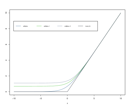
Figure 1: Comparaison between softplus and max(x,0)

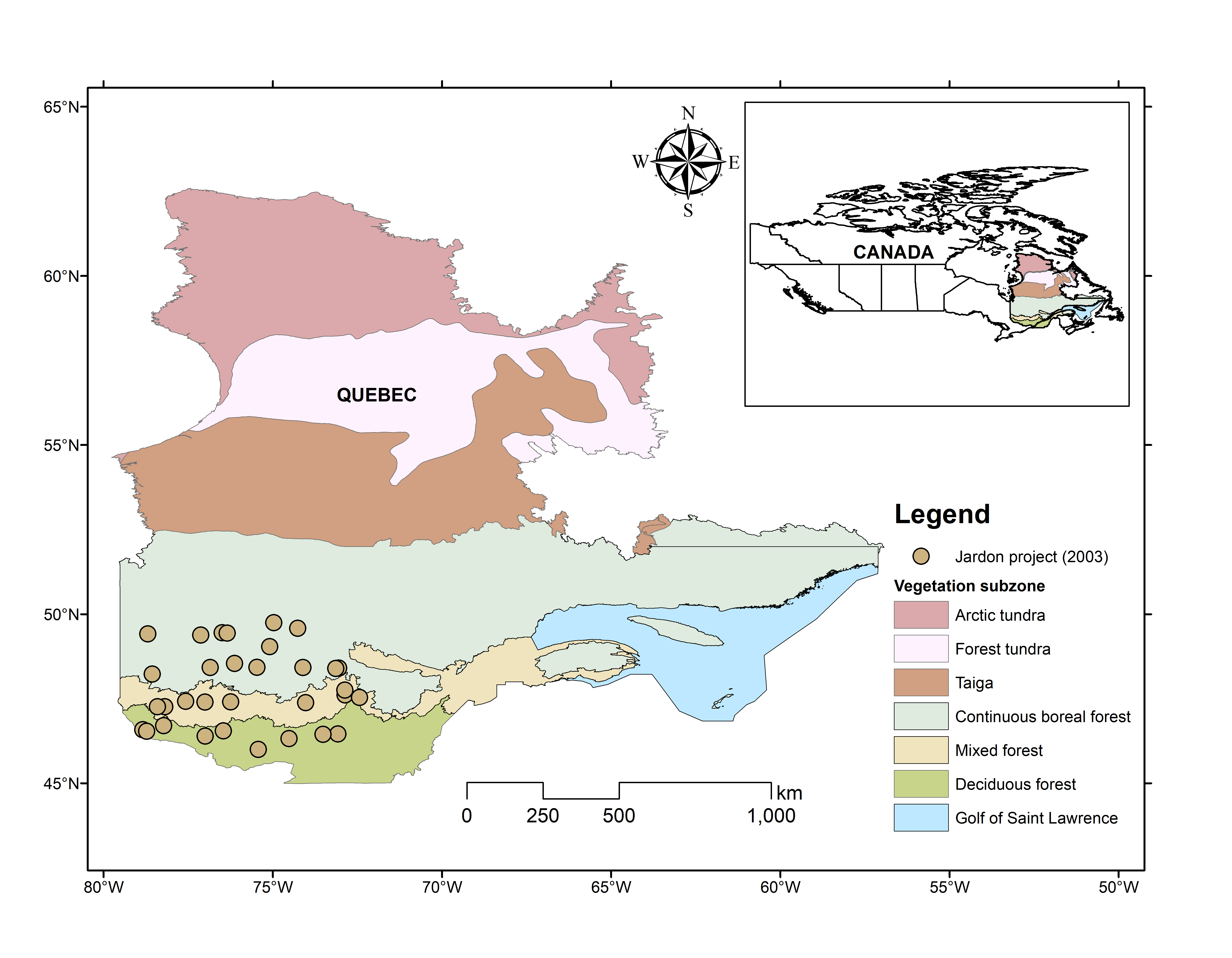
Figure 2: Location of study sites from Jardon Project (2003) in Canadian boreal ecoregions.

(a)

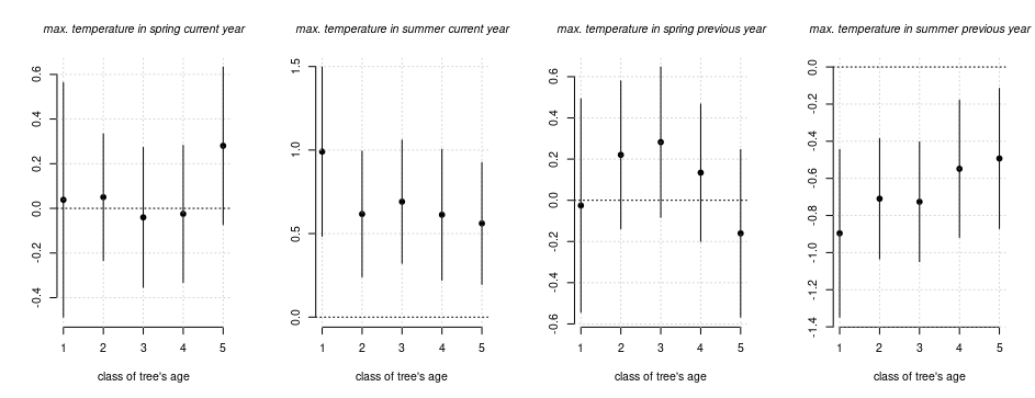
(b)

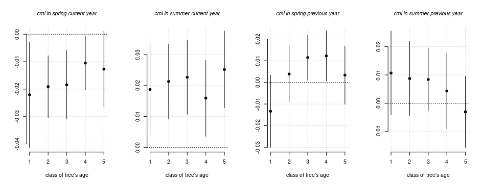
(c)

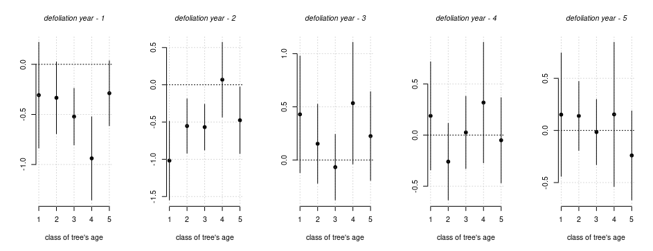
Figure 3: Model with Temperature + CMI + Defoliation. classes of age 1 : < 75, 2 : 75 – 100, 3 : 100 – 125, 4 : 125 – 150 and 5 : > 150 years (a) effects of maximum temperature in spring and summer in current and previous year; (b) effects of cmi index in spring and summer in current and previous year and (c) delayed effect of level of defoliation. The dashed horizontal line corresponds to zero.

(a)

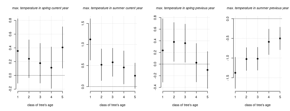
(b)

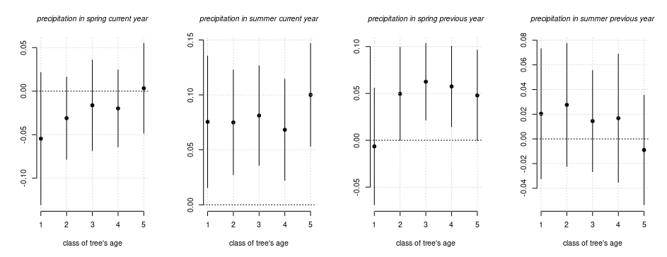
(c)

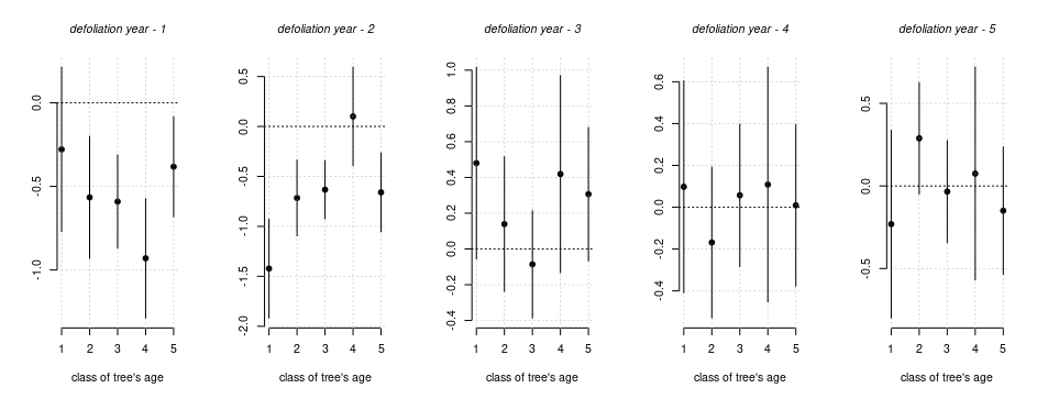
Figure 4: Model with Temperature + Precipitation + Defoliation. classes of age 1 : < 75, 2 : 75 – 100, 3 : 100 – 125, 4 : 125 – 150 and 5 : > 150 years (a) effects of maximum temperature in spring and summer in current and previous year; (b) effects of precipitation index in spring and summer in current and previous year and (c) delayed effect of level of defoliation. The dashed horizontal line corresponds to zero.

References

- Aber et al. (2001) John Aber, Ronald P Neilson, Steve McNulty, James M Lenihan, Dominique Bachelet, and Raymond J Drapek. Forest processes and global environmental change: predicting the effects of individual and multiple stressors: we review the effects of several rapidly changing environmental drivers on ecosystem function, discuss interactions among them, and summarize predicted changes in productivity, carbon storage, and water balance. BioScience, 51(9):735–751, 2001.
- Aknouche and Francq (2020) Abdelhakim Aknouche and Christian Francq. Count and duration time series with equal conditional stochastic and mean orders. Econometric Theory, page 1–33, 2020. doi: 10.1017/S0266466620000134.
- Allen et al. (2010) D.E. Allen, M. McAleer, M. Scharth, University of Canterbury. Department of Economics, and Finance. Realized Volatility Risk. Working paper (University of Canterbury. Department of Economics and Finance). Department of Economics and Finance, College of Business and Economics, University of Canterbury, 2010. URL https://books.google.fr/books?id=YD-RtgEACAAJ.
- Beguería and Vicente-Serrano (2017) Santiago Beguería and Sergio M. Vicente-Serrano. SPEI: Calculation of the Standardised Precipitation-Evapotranspiration Index, 2017. URL https://CRAN.R-project.org/package=SPEI. R package version 1.7.
- Berguet et al. (2021) Cassy Berguet, Maxence Martin, Dominique Arseneault, and Hubert Morin. Spatiotemporal dynamics of 20th-century spruce budworm outbreaks in eastern canada: Three distinct patterns of outbreak severity. Frontiers in Ecology and Evolution, 8, 2021. ISSN 2296-701X. doi: 10.3389/fevo.2020.544088. URL https://www.frontiersin.org/article/10.3389/fevo.2020.544088.
- Bollerslev (1986) T. Bollerslev. Generalized autoregressive conditional heteroskedasticity. Journal of Econometrics, 31:307–327, 1986.
- Boulanger and Arseneault (2004) Yan Boulanger and Dominique Arseneault. Spruce budworm outbreaks in eastern quebec over the last 450 years. Canadian Journal of Forest Research, 34(5):1035–1043, 2004.
- Bunn (2008) Andrew G Bunn. A dendrochronology program library in r (dplr). Dendrochronologia, 26(2):115–124, 2008.
- Camarero et al. (2003) JJ Camarero, E Martín, and E Gil-Pelegrín. The impact of a needleminer (epinotia subsequana) outbreak on radial growth of silver fir (abies alba) in the aragón pyrenees: a dendrochronological assessment. Dendrochronologia, 21(1):3–12, 2003.
- Cameron and Trivedi (2013) A Colin Cameron and Pravin K Trivedi. Regression analysis of count data, volume 53. Cambridge university press, 2013.
- Chan et al. (2020) Bunyeth Chan, Peng Bun Ngor, Zeb S. Hogan, Nam So, Sébastien Brosse, and Sovan Lek. Temporal dynamics of fish assemblages as a reflection of policy shift from fishing concession to co-management in one of the world’s largest tropical flood pulse fisheries. Water, 12(11), 2020. ISSN 2073-4441. doi: 10.3390/w12112974. URL https://www.mdpi.com/2073-4441/12/11/2974.
- Chou et al. (2015) Ray Yeutien Chou, Hengchih Chou, and Nathan Liu. Range volatility: a review of models and empirical studies. Handbook of financial econometrics and statistics, pages 2029–2050, 2015.
- Davis et al. (2016) Richard A Davis, Scott H Holan, Robert Lund, and Nalini Ravishanker. Handbook of discrete-valued time series. CRC Press, 2016.
- Debaly and Truquet (2019) Zinsou Max Debaly and Lionel Truquet. Stationarity and moment properties of some multivariate count autoregressions. arXiv preprint arXiv:1909.11392, 2019.
- Debaly and Truquet (2021) Zinsou Max Debaly and Lionel Truquet. Iterations of dependent random maps and exogeneity in nonlinear dynamics. Econometric Theory, page 1–38, 2021. doi: 10.1017/S0266466620000559.
- Debaly and Truquet (202x) Zinsou Max Debaly and Lionel Truquet. Multivariate time series models for mixed data. to appear in Bernoulli, 202x.
- Dennis and Schnabel (1983) JE Dennis and RB Schnabel. Numerical methods for unconstrained optimization and nonlinear equations prentice-hall. Inc.: Englewood Cli s, 1983.
- Diop and Kengne (2021) Mamadou Lamine Diop and William Kengne. Inference and model selection in general causal time series with exogenous covariates. arXiv preprint arXiv:2102.02870, 2021.
- Engle and Russell (1998) Robert F. Engle and Jeffrey R. Russell. Autoregressive conditional duration: A new model for irregularly spaced transaction data. Econometrica, 66(5):1127–1162, 1998. ISSN 00129682, 14680262. URL http://www.jstor.org/stable/2999632.
- Fleming and Volney (1995) Richard A Fleming and W Jan A Volney. Effects of climate change on insect defoliator population processes in canada’s boreal forest: some plausible scenarios. Water, Air, and Soil Pollution, 82(1):445–454, 1995.
- Gauthier et al. (2015) Sylvie Gauthier, Patrick Bernier, T Kuuluvainen, AZ Shvidenko, and DG Schepaschenko. Boreal forest health and global change. Science, 349(6250):819–822, 2015.
- Girardin et al. (2016) Martin P. Girardin, Olivier Bouriaud, Edward H. Hogg, Werner Kurz, Niklaus E. Zimmermann, Juha M. Metsaranta, Rogier de Jong, David C. Frank, Jan Esper, Ulf Büntgen, Xiao Jing Guo, and Jagtar Bhatti. No growth stimulation of canada’s boreal forest under half-century of combined warming and co2 fertilization. Proceedings of the National Academy of Sciences, 113(52):E8406–E8414, 2016. ISSN 0027-8424. doi: 10.1073/pnas.1610156113. URL https://www.pnas.org/content/113/52/E8406.
- Glorot et al. (2011) Xavier Glorot, Antoine Bordes, and Yoshua Bengio. Deep sparse rectifier neural networks. In Proceedings of the fourteenth international conference on artificial intelligence and statistics, pages 315–323. JMLR Workshop and Conference Proceedings, 2011.
- Guay et al. (1992) Régent Guay, Réjean Gagnon, and Hubert Morin. A new automatic and interactive tree ring measurement system based on a line scan camera. The Forestry Chronicle, 68(1):138–141, 1992.
- Jardon et al. (2003) Yves Jardon, Hubert Morin, and Pierre Dutilleul. Périodicité et synchronisme des épidémies de la tordeuse des bourgeons de l’épinette au québec. Canadian Journal of Forest Research, 33(10):1947–1961, 2003.
- Klapwijk et al. (2013) Maartje J Klapwijk, György Csóka, Anikó Hirka, and Christer Björkman. Forest insects and climate change: Long-term trends in herbivore damage. Ecology and evolution, 3(12):4183–4196, 2013.
- Klimko and Nelson (1978) Lawrence A Klimko and Paul I Nelson. On conditional least squares estimation for stochastic processes. The Annals of statistics, pages 629–642, 1978.
- Krause and Morin (1995) Cornelia Krause and Hubert Morin. Changes in radial increment in stems and roots of balsam fir [abies balsamea (l.) mill.] after defoliation spruce budworm. The forestry chronicle, 71(6):747–754, 1995.
- Krause et al. (2003) Cornelia Krause, F Gionest, Hubert Morin, and David A MacLean. Temporal relations between defoliation caused by spruce budworm (choristoneura fumiferana clem.) and growth of balsam fir (abies balsamea (l.) mill.). Dendrochronologia, 21(1):23–31, 2003.
- Labrecque-Foy et al. (2020) Julie-Pascale Labrecque-Foy, Hubert Morin, and Miguel Montoro Girona. Dynamics of territorial occupation by north american beavers in canadian boreal forests: A novel dendroecological approach. Forests, 11(2):221, 2020.
- Lavoie et al. (2019) Janie Lavoie, Miguel Montoro Girona, and Hubert Morin. Vulnerability of conifer regeneration to spruce budworm outbreaks in the eastern canadian boreal forest. Forests, 10(10):850, 2019.
- Martin et al. (2020) Maxence Martin, Miguel Montoro Girona, and Hubert Morin. Driving factors of conifer regeneration dynamics in eastern canadian boreal old-growth forests. PLoS One, 15(7):e0230221, 2020.
- (33) MFFP. Données sur les perturbations naturelles - insecte : Tordeuse des bourgeons de l’épinette. URL https://www.donneesquebec.ca/recherche/fr/dataset/donnees-sur-les-perturbations-naturelles-insecte-tordeuse-des-bourgeons-de-lepinette. Accessed: 2019-05-19.
- Montoro Girona et al. (2016) Miguel Montoro Girona, Hubert Morin, Jean-Martin Lussier, and Denis Walsh. Radial growth response of black spruce stands ten years after experimental shelterwoods and seed-tree cuttings in boreal forest. Forests, 7(10):240, 2016.
- Montoro Girona et al. (2017) Miguel Montoro Girona, Sergio Rossi, Jean-Martin Lussier, Denis Walsh, and Hubert Morin. Understanding tree growth responses after partial cuttings: A new approach. PLoS One, 12(2):e0172653, 2017.
- Montoro Girona et al. (2018) Miguel Montoro Girona, Lionel Navarro, and Hubert Morin. A secret hidden in the sediments: Lepidoptera scales. Frontiers in Ecology and Evolution, 6:2, 2018.
- Montoro Girona et al. (2019) Miguel Montoro Girona, Hubert Morin, Jean-Martin Lussier, and Jean-Claude Ruel. Post-cutting mortality following experimental silvicultural treatments in unmanaged boreal forest stands. Frontiers in Forests and Global Change, page 4, 2019.
- Morin et al. (2021) Hubert Morin, Réjean Gagnon, Audrey Lemay, and Lionel Navarro. Chapter thirteen - revisiting the relationship between spruce budworm outbreaks and forest dynamics over the holocene in eastern north america based on novel proxies. In Edward A. Johnson and Kiyoko Miyanishi, editors, Plant Disturbance Ecology (Second Edition), pages 463–487. Academic Press, San Diego, second edition edition, 2021. ISBN 978-0-12-818813-2. doi: https://doi.org/10.1016/B978-0-12-818813-2.00013-7. URL https://www.sciencedirect.com/science/article/pii/B9780128188132000137.
- Navarro et al. (2018) Lionel Navarro, Hubert Morin, Yves Bergeron, and Miguel Montoro Girona. Changes in spatiotemporal patterns of 20th century spruce budworm outbreaks in eastern canadian boreal forests. Frontiers in Plant Science, 9:1905, 2018.
- R Core Team (2021) R Core Team. R: A Language and Environment for Statistical Computing. R Foundation for Statistical Computing, Vienna, Austria, 2021. URL https://www.R-project.org/.
- Régnière et al. (2014) Jacques Régnière, Rémi Saint-Amant, Ariane Béchard, and Ahmed Moutaoufik. BioSIM 10: User’s manual. Laurentian Forestry Centre Québec, QC, Canada, 2014.
- Seidl et al. (2017) Rupert Seidl, Dominik Thom, Markus Kautz, Dario Martin-Benito, Mikko Peltoniemi, Giorgio Vacchiano, Jan Wild, Davide Ascoli, Michal Petr, Juha Honkaniemi, et al. Forest disturbances under climate change. Nature climate change, 7(6):395–402, 2017.
- Sim (1990) Chiaw-Hock Sim. First-order autoregressive models for gamma and exponential processes. Journal of Applied Probability, 27(2):325–332, 1990.
- Speer and Kulakowski (2017) James H Speer and Dominik Kulakowski. Creating a buzz: insect outbreaks and disturbance interactions. In Dendroecology, pages 231–255. Springer, 2017.
- Taniguchi and Kakizawa (2002) Masanobu Taniguchi and Yoshihide Kakizawa. Asymptotic theory of statistical inference for time series. Springer Science & Business Media, 2002.
- Vourlitis et al. (2022) George L. Vourlitis, Osvaldo Borges Pinto, Higo J. Dalmagro, Paulo Enrique Zanella de Arruda, Francisco de Almeida Lobo, and José de Souza Nogueira. Tree growth responses to climate variation in upland and seasonally flooded forests and woodlands of the cerrado-pantanal transition of brazil. Forest Ecology and Management, 505:119917, 2022. ISSN 0378-1127. doi: https://doi.org/10.1016/j.foreco.2021.119917. URL https://www.sciencedirect.com/science/article/pii/S0378112721010082.
- Weiß (2018) Christian H Weiß. An introduction to discrete-valued time series, chapter 4. John Wiley & Sons, 2018.