Quantum advantage for multi-option portfolio pricing and valuation adjustments

Abstract

A critical problem in the financial world deals with the management of risk, from regulatory risk to portfolio risk. Many such problems involve the analysis of securities modelled by complex dynamics that cannot be captured analytically, and hence rely on numerical techniques that simulate the stochastic nature of the underlying variables. These techniques may be computationally difficult or demanding. Hence, improving these methods offers a variety of opportunities for quantum algorithms. In this work, we study the problem of Credit Valuation Adjustments (CVAs) which have significant importance in the valuation of derivative portfolios. We propose quantum algorithms that accelerate statistical sampling processes to approximate the CVA under different measures of dispersion, using known techniques in Quantum Monte Carlo (QMC) and analyse the conditions under which we may employ these techniques.

1 Introduction

1.1 Quantitative Finance

Derivatives are financial securities whose value is derived from underlying asset(s). The derivatives market has seen a rapid expansion and is estimated to be up to more than ten times of the global Gross Domestic Product [29]. Financial theory has co-evolved with this expansion. A derivative contract typically consists of payoff functions that are often dependent upon market state variables realised in the future, which are necessarily random. Study of these random variables and accurately pricing these financial contracts is the principle task of quantitative finance, which lends itself to theoretical treatment using measure and probability theory, stochastic processes, and numerical methods. In particular, the evolution of the underlying assets are modelled as Ito processes [28], and may be analysed under the settings of stochastic calculus. The evolution of the price process then can be modelled using stochastic differential equations (SDEs).

Unfortunately, analytical solutions are often not known or are prohibitively complex to formulate, especially when one considers the interactions between a basket of derivative contracts. Such complications are the main reasons why Monte Carlo engines have become an integral part of financial modelling, providing a general, numerical approach to obtain solutions to compute expectations of random variables even in high dimensional settings.

In cases when an analytical solution is possible, derivative products may be valued by the distinguished Black-Scholes-Merton (BSM) [4] formula. However, this formula makes a set of well-known but limiting assumptions. Of primary concern to the dealing house involved in the transaction of financial derivatives may be outlined; to what extent should the valuation of derivative portfolios go beyond the BSM model based on the idiosyncratic characteristics of the parties in question? Such a question is answered in reality by the practice of XVAs, where the ‘X’ refer to a number of items such as Credit (C), Debt (D), Funding (F), Margin (M), Capital Valuation (K) and the ‘VA’ referring to Valuation Adjustments [15]. Each term pertains to one of credit, funding and regulatory capital requirements that detracts the adjusted derivative portfolio value from the BSM price. Further elaborations on the CVA problem and the role of XVA desks are presented in Appendix A.

Our examination in particular concerns the credit component, also known as CVA. While the collapse of Lehman Brothers [3] is likely the most ill-famed credit event in popular culture, credit events are anything but a rare occurrence in finance. The credit crisis of 2007 and collapse of Lehman Brothers in 2008 brought to attention systemic risks in the financial markets and the need for better modelling of risks. In response, regulatory frameworks have been developed by the Basel Committee on Banking Supervision to mitigate further risks of financial crisis. Despite stricter controls and updates to the theory of derivative pricing, the market still differs significantly in pricing practice [31] with XVA desks applying varying levels of adjustments. This is attributed to the complexity of the modelling and controversial modelling standards, resulting in divergent prices and two-tier markets. Failure to accurately model these risks have resulted in large losses. The blowup of Archegos Capital in March 2021 is an example of institutional failure to accurately price counterparty credit risk, and the losses incurred by the likes of Credit Suisse and Nomura Holdings evidence the consequences [14]. It follows that our subject of interest is of critical importance in both methodology and implementation therein.

1.2 Quantum algorithms

Quantum computing exploits quantum mechanical phenomena such as superposition and entanglement to perform computation on quantum states formed by quantum bits (qubits). In some cases, quantum algorithms promise speedups over their classical counterparts. An example is the integer factoring problem, where the Shor’s algorithm [27] allows an exponential speedup over classical algorithms in the factorization of integers. Another useful algorithm in search problems under the quantum setting is known as the Grover’s search, [16], that allows the search for specific data in an unstructured table using $\mathcal{O}\left(\sqrt{N}\right)$ queries, promising quadratic speedups to the best classical counterpart.

Another commonly known algorithm that is particularly useful is called the Quantum Amplitude Estimation (QAE) [6], which estimates the amplitude of some arbitrary quantum state $|{\psi}\rangle$ in a subspace of the state space. Generalising QAE and other useful algorithms [13] as a subroutine, developments in Quantum Monte Carlo (QMC) techniques [22] have been discussed.

Several works consider the application of quantum computing in finance. A general review of the today’s challenges in quantum finance can be found [5], where additional literature such as quantum linear algebra, and quantum machine learning are discussed.

1.3 Monte Carlo methods and their quantum counterparts

Monte Carlo is a statistical sampling method used to estimate properties of statistical distributions that are difficult to estimate analytically. Consider a non-empty set of random variables $S$ each from some, not necessarily identical, distribution. Let $g$ be a Borel-measurable function over $S$ on $\mathbb{R}$. Our objective is to find $\mu$, the population mean $\mathbbm{E}\left(g(S)\right)$. We can calculate $\bar{x}$, the sample average as an estimate of $\mu$ via statistical sampling. Assuming that the variance is bounded by $\sigma^{2}$, Chebyshev’s inequality guarantees an upper bound on the probability of the accuracy of our estimate $\bar{x}$ up to error $\epsilon$, such that $\mathbbm{P}\left[|\bar{x}-\mu|\geq\epsilon\right]\leq\frac{\sigma^{2}}{n\epsilon^{2}}$. The statistical exhibit of quadratic dependence on $\frac{\sigma}{\epsilon}$ is less than desirable, since the number of samples required to obtain an estimate up to additive error of $\epsilon$ is $n\in\mathcal{O}\left(\frac{\sigma^{2}}{\epsilon^{2}}\right)$. Notably, Montanaro’s [22] work demonstrates the near quadratic speed up over best classical methods in the estimation of output values of arbitrary randomized algorithms in the general settings for QMC, the results of which we consider extensively useful for application in the financial setting.

1.4 Literature on CVA and relevant work

Until recently, little to no known literature expounded upon quantizing the CVA computation. The recent works [1] in May of 2021 demonstrated the first attempt of quantizing the CVA formula, introducing numerous heuristics and adoption of QAE variants to reduce circuit depth and resource requirements for implementations on near-term quantum devices. In particular, a Bayesian variant using engineered likelihood functions were explored, while using standard techniques for accelerating Monte Carlo sampling techniques by Montanaro. Under classical settings, the classical counterpart of the Monte Carlo engines are used to approximate CVA computations [15]. However, alternative proposals such as the use of neural networks have been proposed [26].

Using the approximation of partition functions to demonstrate speedups in multiple stage Markov chain Monte Carlo techniques, Montanaro’s work extends previous works [17] to reduce the number of repetitions required to estimate an observable up to a desired accuracy in general settings. Since then, new research has found improvements in the quantum advantage for multilevel Monte Carlo methods for SDEs found in mathematical finance [2], as well as for quantum multi-variate Monte Carlo problems. [11]. However, there is no known literature of the applications of such findings under the CVA setting.

1.5 Our results

We find that under guarantees of a bounded variance in the CVA, we may provide better results for approximating the CVA value than the general settings [1]. We find that such guarantees are reasonably common and useful in practical settings. In particular, we may obtain an approximation of the CVA value up to desired additive error $\epsilon$ using $\mathcal{T}_{\rm CVA}\in\mathcal{O}\left(\frac{\sigma}{\epsilon}\log^{\frac{3}{2}}{\frac{\sigma}{\epsilon}}\log{\log{\frac{\sigma}{\epsilon}}}\log{\frac{1}{\delta}}\right)$ queries and $\tilde{\mathcal{O}}\left(T_{\rm CVA}\right)$ gates with success probability $1-\delta$. See Theorem 5 for a precise statement of this result.

Additionally, if we are given a variance bound such that $\mathrm{Var}(CVA)\leq B\cdot\mathbb{E}[{CVA}]^{2}$ for some $B>0$, then we may obtain an approximation of the CVA value up to desired relative error $\epsilon$ using $\mathcal{O}\left(\frac{B}{\epsilon}\log^{\frac{3}{2}}{\frac{B}{\epsilon}}\log{\log{\frac{B}{\epsilon}}}\log{\frac{1}{\delta}}\right)$ queries and $\tilde{\mathcal{O}}\left(\frac{B}{\epsilon}\log^{\frac{3}{2}}{\frac{B}{\epsilon}}\log{\log{\frac{B}{\epsilon}}}\log{\frac{1}{\delta}}\right)$ gates with success probability $1-\delta$. See Theorem 6 for a precise statement of this result. We compare these algorithms to the setting where no variance guarantees can be obtained.

1.6 Organization of this work

In Section 1, we give primary concerns commonly occurring in the area of modern finance, and introduce derivative products and highlight the need for taking into account adjustments for counterparty risks. We give an overview of quantum algorithms, Monte Carlo approaches and relevant literature. We then discuss preliminaries and notations required for formalising and introducing our problem settings in Section 2. We provide formal definitions for the multi-option pricing problem and the CVA problem in Sections 3, where we see that the CVA problem can be framed as a variant of the multi-option pricing problem. We discuss quantum subroutines and relevant theory in Section 4. In Section 5, we argue that the solutions to the problem statements may be found using these algorithms. We conclude and provide some guidance for possible future work in Section 6. In the Appendix A, we discuss more on CVAs and provide the derivation of the CVA formula. We discuss relevant quantitative finance topics in Appendix B.

2 Preliminaries

In this section we discuss notations and definitions.

2.1 Mathematical preliminaries

The following are mathematical notations and definitions used in discussions throughout the paper.

Matrix Vectorization $-$ For any matrix $A=(\bm{a}_{1},\cdots,\bm{a}_{m})$ with columns $a_{j},\forall j\in[m]$, define the vector constructed by stacking the columns of $A$ as ${\rm vec}(A)$ as the vectorization of a matrix.

In our work, when working with numbers in the classical setting, we assume an arithmetic model with no encoding errors. Additionally, arithmetic operations all cost $\mathcal{O}\left(1\right)$ time. When working with operations in the quantum setting, we use the fixed-point encoding as defined below, and also assume an arithmetic model with no encoding errors and $\mathcal{O}\left(1\right)$ time.

Definition 1 (Notation for fixed-point encoding of real numbers).

Let $c_{1},c_{2}$ be positive integers and $a\in\{0,1\}^{c_{1}}$ and $b\in\{0,1\}^{c_{2}}$ be bit strings. Define the rational number

$$\mathcal{Q}(a,b) := a_{c_{1}}\cdots a_{1}.b_{1}\cdots b_{c_{2}}$$

$$= 2^{c_{1}-1}a_{c_{1}}+\cdots+2a_{2}+a_{1}+\frac{1}{2}b_{1}+\cdots+\frac{1}{2^{c_{2}}}b_{c_{2}}\in\left[0,\frac{2^{c_{1}+c_{2}}-1}{2^{c_{2}}}\right]$$

Consider an arbitrary, positive finite number $x\in\mathbb{R}^{+}$ that may be encoded up to desired accuracy by appropriate choices of $c_{1},c_{2}$. Define the short-hand notation

$$\mathcal{Q}(z):=\mathcal{Q}(a,b)$$

where $z:=(c_{1},c_{2})\in\{0,1\}^{c_{1}+c_{2}}$. For any real number $r\in[0,2^{c_{1}}]$ there exist $a\in\{0,1\}^{c_{1}}$ and $b\in\{0,1\}^{c_{2}}$ such that the difference to $\mathcal{Q}(a,b)$ is at most $\frac{1}{2^{c_{2}+1}}$. Given a vector of bit strings $v\in(\{0,1\}^{c})^{n}$, the notation $\mathcal{Q}(v)$ means the vector of $\mathcal{Q}(v_{j})$.

$\ell_{1}$-norm of vectors $-$ Let $c$ be a positive integer and $v\in(\{0,1\}^{c})^{n}$ be an $n$-dimensional vector of bit strings. We denote by $\|v\|_{1}$ the $\ell_{1}$-norm of the vector, defined as $\sum^{n}_{i=1}|\mathcal{Q}(v_{i})|$. Recall that we have defined the notation $\mathcal{Q}(v)$ to be the vector of $\mathcal{Q}(v_{j})$. As such, we use the notations $\|v\|_{1}$ and $\|\mathcal{Q}(v)\|_{1}$ interchangeably where convenient.

Inner products $-$ Let there be two vectors $u\in(\{0,1\}^{c_{1}})^{N}$, $v\in(\{0,1\}^{c_{2}})^{N}$, such that $\mathcal{Q}(u)\in[0,2^{c_{1}}),\mathcal{Q}(v)\in[0,2^{c_{2}})$. Then $u\cdot v$ is the inner product representing $\sum^{N}_{j=1}\mathcal{Q}(u_{j})\mathcal{Q}(v_{j})$.

In our work, we assume that we have access to vector components under different configurations. Here, we define the access to elements of a vector in the classical setting under the query access model and the sampling access model.

Definition 2 (Vector access).

Let $c$ and $n$ be two positive integers and $\bm{u}$ be a vector of bit strings $\mathbf{u}\in(\{0,1\}^{c})^{n}$. We say that we have access to a vector $\bm{u}$ if we have access to the mapping $j\to\bm{u}_{j}$. We denote this access by $\bm{VA}(\bm{u},n,c)$ and the time for a query by $\mathcal{T}_{\bm{VA}(\bm{u},n,c)}$. When there is no ambiguity of the inputs, we use the shorthand notation $\bm{VA}(\bm{u})$.

Definition 3 (Sampling access).

Let $c$ and $n$ be two positive integers and $\bm{v}$ be a vector of bit strings $\mathbf{v}\in(\{0,1\}^{c})^{n}$. We say we have sampling access to $\bm{v}$ if we can draw a sample $j\in[n]$ with probability $\mathcal{Q}(v_{j})/\|\mathcal{Q}(v)\|_{1}$. We denote this access by $\bm{SA}(\bm{v},n,c)$ and each access costs $T_{\bm{SA}(\bm{v},n,c)}$. When there is no ambiguity of the inputs, we use the shorthand notation $\bm{SA}(\bm{v})$.

We make use of quantum subroutines in our work to perform sampling on vector elements for inner product estimations. The classical analogue is presented in the following Lemma 1, which has been adapted from [30] and written as in [25].

Lemma 1 (Inner product with $\ell_{1}$-sampling).

Let $\epsilon,\delta\in(0,1)$. Given query access to $\bm{v}\in\mathbbm{R}^{n}$ and $\bm{SA}(\bm{u})$ access to $\bm{u}\in\mathbbm{R}^{n}$, we can determine $\bm{u}\cdot\bm{v}$ to additive error $\epsilon$ with success probability at least $1-\delta$ with $\mathcal{O}\left(\frac{\|\bm{u}\|_{1}^{2}\|\bm{v}\|_{\max}^{2}}{\epsilon^{2}}\log\frac{1}{\delta}\right)$ queries and samples, and $\tilde{\mathcal{O}}\left(\frac{\|\bm{u}\|_{1}^{2}\|\bm{v}\|_{\max}^{2}}{\epsilon^{2}}\log\frac{1}{\delta}\right)$ time complexity.

Proof.

Define a random variable $Z$ with outcome ${\rm sgn}(u_{j})\|\bm{u}\|_{1}v_{j}$ with probability $|u_{j}|/\|\bm{u}\|_{1}$. Note that $\mathbbm{E}[Z]=\sum_{j}{\rm sgn}(u_{j})\|\bm{u}\|_{1}v_{j}|u_{j}|/\|\bm{u}\|_{1}=\bm{u}\cdot\bm{v}$. Also,

$$\mathbbm{V}[Z]\leq\mathbbm{E}[Z^{2}]=\sum_{j}\|\bm{u}\|_{1}^{2}v_{j}^{2}|u_{j}|/\|\bm{u}\|_{1}\leq\|\bm{u}\|_{1}^{2}\|\bm{v}\|_{\max}^{2}.$$

Take the median of $6\log 1/\delta$ evaluations of the mean of $9\|\bm{u}\|_{1}^{2}\|\bm{v}\|_{\max}^{2}/(2\epsilon^{2})$ samples of $Z$. Then, by using the Chebyshev and Chernoff inequalities, we obtain an $\epsilon$ additive error estimation of $\bm{u}\cdot\bm{v}$ with probability at least $1-\delta$ in $\mathcal{O}\left(\frac{\|\bm{u}\|_{1}^{2}\|\bm{v}\|_{\max}^{2}}{\epsilon^{2}}\log\frac{1}{\delta}\right)$ queries. ∎

2.2 Probability preliminaries

To aid in the formal treatment of derivative pricing and CVA concepts, we introduce relevant concepts in probability theory required to construct arguments on asset price dynamics.

Probability Spaces and Filtrations $-$ We denote an arbitrary probability space $(\Omega,\mathcal{F},\mathbbm{Q})$ where $\Omega$ is a non-empty sample space, $\mathcal{F}$ the filtration and $\mathbbm{Q}$ the probability measure. Consider for some fixed, positive integer $T$, we let $\mathcal{F}_{t},0\leq t\leq T$ be a filtration of sub-$\sigma$ algebras of $\mathcal{F}$. We may take $\mathcal{F}_{t}$ then to be market state variables and information available up to time $t$.

Stochastic Processes $-$ Consider a collection of random variables $V_{t}$ and a collection of sigma algebras $\mathcal{F}_{t},0\leq t\leq T$, for which $\mathcal{F}_{0}\subseteq\mathcal{F}_{1}\subseteq\cdots\subseteq\mathcal{F}_{T-1}\subseteq\mathcal{F}_{T}$, corresponding to a non-empty sample space $\Omega$ for a fixed positive integer $T$. The collection of random variables denoted by $V$ and indexed by $t$ is an adapted stochastic process if $\forall t\in[T]$, $V_{t}$ is $\mathcal{F}_{t}$ measurable.

Probability Measures $-$ Consider two random variables $X,Y:\Omega\to\mathbb{R}$ taking some real values. Let $\mathbbm{Q}$ be the joint distribution measure for $(X,Y)$, then we have $\mathbbm{Q}((X,Y)\in\mathbbm{C})$ defined for all Borel sets $\mathbbm{C}\subset\mathbbm{R}^{2}$. Further assume that $X$ and $Y$ are independent. Then, their distribution measure factors into $\mathbbm{Q}_{X}\left(X\in\mathbbm{C}\right)$ and $\mathbbm{Q}_{Y}\left(Y\in\mathbbm{C}\right)$.

2.3 Financial preliminaries

The derivative pricing and CVA problem relates different variables from both financial theory and contractual agreement; here we discuss some of these variables involved in such computations.

Portfolio Process $-$ Assume a probability space $(\Omega,\mathcal{F},\mathbbm{Q})$, where $\Omega$ is the set of economic events, $\mathcal{F}$ is the sigma algebra for $\Omega$, and a probability measure $\mathbbm{Q}$. Let $T$ be a fixed, positive integer denoting the number of time steps in the model economy. We let $\mathcal{F}_{t},0\leq t\leq T$ be a filtration of sub-$\sigma$ algebras of $\mathcal{F}$, where $\mathcal{F}_{0}\subseteq\mathcal{F}_{1}\subseteq\cdots\subseteq\mathcal{F}_{T}=\mathcal{F}$. Define the discounted portfolio value (of a single derivative or a basket of derivatives) to be a random variable $V:\Omega\to[0,\infty)$. Let $V_{t}$ be a $\mathcal{F}_{t}$ measurable adapted stochastic process, representing the discounted portfolio value at time $t$, $\forall t\in[T]$.

There are numerous events that can lead to a credit event, and of the most common nature may be attributed to operations of financially unsound nature. We formally define the concepts of random variables on default times, survival probabilities and the recovery rates for a counterparty trade.

Credit/Default Event $-$ Let $\tau:\Omega\to[T]\cup\{\infty\}$ be the random variable for the time of a credit event (e.g., a bankruptcy). The list of credit events include but are not limited to those outlined by the International Swaps and Derivatives Association [19]. Further discussions on Financial Law is not discussed as it is not central to our work.

Default Probabilities $-$ Let $\phi:\{t:t\in[T]\cup\{\infty\}\}\to[0,1)$ be the cumulative distribution function for credit default, such that $\phi(\tau<t)$ is the probability that some counterparty in concern defaults at time prior to $t$. $\phi$ shall be defined in the range of $\tau$, the time of a credit event. Without ambiguity, define $\phi(t_{i}\leq\tau\leq t_{j}):=\phi(t_{j})-\phi(t_{i})$ to be the probability of default between two time instances over the domain $[T]$, where $t_{i}\leq t_{j}$. The default probabilities may be obtained by bootstrapping hazard rates from the Credit Default Swap (CDS) market. The CDS market is said to ‘imply’ default probabilities and may be obtained under the risk-neutral measure. For a more detailed explanation on deriving default probabilities from the CDS curve, refer to Appendix B.1.

Recovery Rate $-$ Let $R\in(0,1)$ be the Recovery Rate, a percentage of the value of the portfolio that may be expected to be recovered in the event of default of the counterparty. The percentage $(1-R)$ can then be defined as the Loss Given Default $(LGD)$, representing as percentage of the positive exposure subject to loss under default.

Discounting $-$ Let $r_{t}\in(0,1)$ be the short rate at time $t$ used to obtain the present value of undiscounted, future valuations of the derivative portfolio. The short rates may be defined to be a deterministic constant or a stochastic process calibrated to the interest rate term structure, to take into account the risk-free interest that may be earned on investing in the money market account or an equivalent choice of numeraire. For a more detailed explanation on interest rate term structures, refer to Appendix B.2. Denote $V^{\prime}_{t}$ as the future value of the portfolio value at time $t$, then we have $V_{t}=\exp\{-\int^{t}_{0}r_{u}du\}V^{\prime}_{t}$.

2.4 Quantum preliminaries

Quantum query (multiple) access $-$ We define quantum query access for obtaining the superposition over elements of a vector.

Definition 4 (Quantum query access).

Let $c$ and $n$ be two positive integers and $\bm{u}$ be a vector of bit strings $\mathbf{u}\in(\{0,1\}^{c})^{n}$. We say that we have quantum access to $\bm{u}$ for $j\in[n]$, if, for arbitrary $b\in\{0,1\}^{c}$,

$$|{j}\rangle|{b}\rangle\to|{j}\rangle|{b\oplus u_{j}}\rangle.$$ (2)

We denote this access by $\bm{QA}(\bm{u},n,c)$. Denote the time for a query by $\mathcal{T}_{\bm{QA}(\bm{u},n,c)}$. When there is no ambiguity of the inputs, we use the shorthand notation $\bm{QA}(\bm{u})$. The quantum oracle query on a superposition follows directly $\sum^{n}_{j=1}|{j}\rangle|{0^{c}}\rangle\to\sum^{n}_{j=1}|{j}\rangle|{u_{j}}\rangle$.

Definition 5 (Quantum matrix access/Quantum multi-vector access).

Let $c$, $n$, and $m$ be positive integers and $\bm{u}_{1},\cdots,\bm{u}_{m}$ be $m$ vectors of bit strings $\in(\{0,1\}^{c})^{n}$. We say that we have quantum access to the matrix $A:=(\bm{u}_{1},\cdots,\bm{u}_{m})$ if we have access to $\bm{QA}({\rm vec}(A))$. Note that we can interpret this access as a superposition access to the set of inputs $\bm{QA}(\bm{u}_{1}),$ $\cdots,$ $\bm{QA}(\bm{u}_{m})$. It allows the operation $|{i}\rangle|{j}\rangle|{0^{c}}\rangle\to|{i}\rangle|{j}\rangle|{(\bm{u}_{i})_{j}}\rangle$, for $i\in[m]$ and $j\in[n]$.

Quantum sampling (multiple) access $-$ We define quantum sampling access into a superposition of eigenstates, where the probability of observing $j$ under a measurement corresponds to the square of its amplitude.

Definition 6 (Quantum sample access).

Let $c$ and $n$ be two positive integers and $\bm{v}$ be a vector of bit strings $\mathbf{v}\in(\{0,1\}^{c})^{n}$. Define quantum sample access to $\bm{v}$ via the operation

$$|{\bar{0}}\rangle\to\frac{1}{\sqrt{\|\mathcal{Q}(v)\|_{1}}}\sum_{j=1}^{n}\sqrt{\mathcal{Q}(v_{j})}|{j}\rangle.$$ (3)

We denote this access by $\bm{QS}(\bm{v},n,c)$. Denote the time for a query by $\mathcal{T}_{\bm{QS}(\bm{v},n,c)}$. When there is no ambiguity of the inputs, we use the shorthand notation $\bm{QS}(\bm{v})$.

Definition 7 (Quantum multi-sample access).

Let $c$, $n$, and $T$ be positive integers and $\bm{v}_{1},\cdots,\bm{v}_{T}$ be $T$ vectors of bit strings $\in(\{0,1\}^{c})^{n}$. Define quantum multi-sample access to $V:=(\bm{v}_{1},\cdots,\bm{v}_{T})$ via the operation

$$|{\bar{0}}\rangle\to\sum_{i=1}^{T}\sum_{j=1}^{n}\sqrt{\frac{\mathcal{Q}((\bm{v}_{i})_{j})}{\|\mathcal{Q}(\rm vec(\bm{V}))\|_{1}}}|{i}\rangle|{j}\rangle.$$ (4)

We denote this access by $\bm{QS}({\rm vec}(V),nT,c)$. Denote the time for a query by $\mathcal{T}_{\bm{QS}({\rm vec}(V),nT,c)}$. When there is no ambiguity of the inputs, we use the shorthand notation $\bm{QS}(\{\bm{v}_{i}\}_{i\in[T]})$.

We note that this is just an instance of the Definition 6. Consider the vectorization $\rm{vec}(V)$, the column vector of dimension $nT$. Now consider the $\bm{QS}({\rm vec}(V))$, which by definition provides the access:

$$|{\bar{0}}\rangle \to \frac{1}{\sqrt{\|\mathcal{Q}(\rm{vec}(V))\|_{1}}}\sum_{k=1}^{nT}\sqrt{\mathcal{Q}(\rm{vec}(V)_{k})}|{k}\rangle$$ (5)

$$= \frac{1}{\sqrt{\sum_{k=1}^{nT}|\mathcal{Q}(\rm{vec}(V)_{k})}|}\sum_{i=1}^{T}\sum_{j=1}^{n}\sqrt{\mathcal{Q}(v_{ij})}|{i}\rangle|{j}\rangle$$ (6)

$$= \frac{1}{\sqrt{\sum^{T}_{i=1}\sum^{n}_{j=1}|\mathcal{Q}(\bm{v}_{ij})|}}\sum_{i=1}^{T}\sum_{j=1}^{n}\sqrt{\mathcal{Q}(v_{ij})}|{i}\rangle|{j}\rangle$$ (7)

We note the fact that any classical circuit can be implemented by an equivalent, reversible quantum circuit of unitary mappings.

Fact 1 (Reversible Logic Synthesis [23]).

Given any classical arithmetic computation implemented by $\mathcal{T}_{cl}$ gates, we may implement an equivalent quantum circuit using $\tilde{\mathcal{O}}\left(\mathcal{T}_{cl}\right)$ gates.

For instance, for an arbitrary vector $V\in\mathbb{R}^{n}$, the classical operation $\max(V,0)$ can be implemented using quantum circuits.

Lemma 2.

Let $c,n$ be two positive integers such that $V\in\mathbb{R}^{n}$ and $\forall v\in V$, $v$ may be represented up to desired accuracy using fixed point encoding as in Definition 1. Then, $\forall v\in V$, $v$ may be decomposed into a difference between two non-negative components such that $v=(v)^{+}-(v)^{-}$ represent the positive and negative values. Assume quantum oracle access $\bm{QA}(V)$. We may obtain $\bm{QA}((V)^{+})$ using two queries to $\bm{QA}(V)$ and additional quantum circuits of depth $\mathcal{O}\left(c\right)$.

Proof.

Consider the element wise operations

$$|{j}\rangle|{\bar{0}}\rangle|{\bar{0}}\rangle \to |{j}\rangle|{v_{j}}\rangle|{\bar{0}}\rangle\to\begin{dcases}|{j}\rangle|{v_{j}}\rangle|{v_{j}}\rangle,&\text{if }\mathcal{Q}(v_{j})\geq 0\\ |{j}\rangle|{v_{j}}\rangle|{\bar{0}}\rangle,&\text{otherwise}\end{dcases}$$ (8)

$$\to \begin{dcases}|{j}\rangle|{\bar{0}}\rangle|{v_{j}}\rangle,&\text{if }\mathcal{Q}(v_{j})\geq 0\\ |{j}\rangle|{\bar{0}}\rangle|{\bar{0}}\rangle,&\text{otherwise}\end{dcases}$$ (9)

This achieves

$$|{j}\rangle|{\bar{0}}\rangle \to \begin{dcases}|{j}\rangle|{v_{j}}\rangle,&\text{if }\mathcal{Q}(v_{j})\geq 0\\ |{j}\rangle|{\bar{0}}\rangle,&\text{otherwise}\end{dcases}$$ (11)

which is by definition $\bm{QA}(\max(v,0))$. ∎

Similarly, for arbitrary $x\in\mathbb{R}$ and $S\subseteq\mathbb{R}$, we may implement the classical operation $f(x)=x\cdot{\mathbbm{1}\{x\in S\}}$ using quantum circuits.

Definition 8 (Quantum comparators).

Let $c,n$ be positive integers, $l$ be a non-negative integer and $\bm{u}$ be a vector of bit strings $\mathbf{u}\in(\{0,1\}^{c})^{n}$. Define element-wise bounded quantum access to $\bm{u}$ for $j\in[n]$ by the operation

$$|{\tilde{l}}\rangle|{u_{j}}\rangle|{\bar{0}}\rangle\to\begin{dcases}|{\tilde{l}}\rangle|{u_{j}}\rangle|{u_{j}}\rangle,&\text{if }l=0,0\leq\mathcal{Q}(u_{j})<1\\ |{\tilde{l}}\rangle|{u_{j}}\rangle|{u_{j}}\rangle,&\text{if }l>0,2^{l-1}\leq\mathcal{Q}(u_{j})<2^{l}\\ |{\tilde{l}}\rangle|{u_{j}}\rangle|{\bar{0}}\rangle,&\text{otherwise}\end{dcases}$$ (13)

on $\mathcal{O}\left(l+c\right)$ qubits, where $\tilde{l}$ is the bit string representation of $2^{l}$. We denote this access by $\bm{QC}(\bm{u},n,c,l)$. Denote the time for a query by $\mathcal{T}_{\bm{QC}(\bm{u},n,c,l)}$. When there is no ambiguity of the inputs, we use the shorthand notation $\bm{QC}(\bm{u},l)$.

Quantum controlled rotations $-$ We define quantum controlled rotations of bounded input states into amplitudes.

Definition 9 (Quantum controlled rotation).

Let $c$ be a positive integer such that $u\in\{0,1\}^{c}$ and $\mathcal{Q}(u)\in[0,1]$. Define quantum controlled rotation as the operation

$$|{u}\rangle|{0}\rangle\to\left(\sqrt{1-\mathcal{Q}(u)}|{0}\rangle+\sqrt{\mathcal{Q}(u)}|{1}\rangle\right)$$ (14)

The cost of this operation depends directly on the precision of our fixed point arithmetic model as in Definition 1. In particular, we neglect the cost of $\mathcal{O}\left(c\right)$ in our computational model and assume this to be of unit cost in the following discussions.

3 Problem Statements

In this section we formalise the multi-option pricing problem and the CVA problem.

3.1 Problem statements for multi-option pricing

In this section we introduce the pricing problem for the general case of a basket of derivatives, and formalise the classical and quantum context in which we might analyse the problem.

A fairly general classical multi-option problem may be phrased as follows. We have a probability space $(\Omega,\Sigma,\mathbbm{Q})$, where $\Omega$ is the set of economic events, $\Sigma$ is the sigma algebra for $\Omega$, and a probability measure $\mathbbm{Q}$. We are given a portfolio of $K$ options or other financial derivatives. For each option, we have a discounted payoff $V^{(k)}:\Omega\to[0,\infty)$. The price of each option is computed by $\mathbbm{E}_{\mathbbm{Q}}\left[V^{(k)}\right]$. The problem is to determine the total portfolio value $\sum_{k=1}^{K}\mathbbm{E}_{\mathbbm{Q}}\left[V^{(k)}\right]$. In this work, we focus on a more specialized problem. We are given a portfolio of $K$ options or other financial derivatives, which we can price independently.

Problem 1 (Classical multi-option pricing problem under independent, finite settings).

Let $K$ be a positive integer for the number of financial derivatives. Assume exists a known integer $n$, such that for each option indexed by $k\in[K]$ we have a probability space $(\Omega^{(k)},\Sigma^{(k)},\mathbbm{Q}^{(k)})$, where $\Omega^{(k)}=\{x:x\in\{0,1\}^{n}\}$ describes the set of economic events, $\Sigma^{(k)}$ the sigma algebra for $\Omega^{(k)}$, and the probability measure is $\mathbbm{Q}^{(k)}$. The probability measures are given via $\bm{VA}(q^{(k)})$ access to the vectors $q^{(k)}\in[0,1]^{N}$ for which $N=2^{n}$ and $\sum_{j=1}^{N}q_{j}^{(k)}=1$. Each option is defined via a discounted payoff $V^{(k)}:\Omega^{(k)}\to[0,\infty)$, for which we are given the vector access $\bm{VA}\left(V^{(k)}\right)$. The price of each option shall be computed by

$$\mathbbm{E}_{q^{(k)}}\left[V^{(k)}\right]=\sum_{j=1}^{N}q^{(k)}_{j}V^{(k)}_{j}.$$ (15)

Define the random variable of the total portfolio value ${\rm TV}:=\sum_{k=1}^{K}V^{(k)}$. The task is to evaluate

$$\mathbbm{E}_{q^{(1)}\cdots q^{(K)}}\left[{\rm TV}\right]=\sum_{k=1}^{K}\mathbbm{E}_{q^{(k)}}\left[V^{(k)}\right].$$ (16)

We note that in this previous problem, when we select a single probability, we select a certain $k\in[K]$ and then a certain index $j\in[N]$ to obtain $q^{(k)}_{j}$. The natural quantum extension of this process is to be able to query both the index $k$ and the index $j$ in superposition. This ability is embodied in the next definition of the quantum version of the same problem.

Problem 2 (Quantum multi-option pricing problem under independent, finite settings).

Let $c$ be a chosen, positive integer and $\forall j,k,V^{(k)}_{j}\in[0,\infty)$ may be represented up to desired accuracy using fixed point encoding as in Definition 1. Given the setting in Problem 1, define the matrices $Q:=\left(q^{(1)},\cdots,q^{(K)}\right)$ and $V:=\left(V^{(1)},\cdots,V^{(K)}\right)$, and assume quantum matrix access $\bm{QA}({\rm vec}(Q))$ and $\bm{QA}({\rm vec}(V))$.

3.2 Problem statements for CVA

We may view CVA as an adjustment of the marked-to-market value of a derivative portfolio to account for counterparty credit risk, which can be calculated as the difference between the risk-free portfolio value proposed by the BSM model and its value taking into account the possibility of default. We shall take them as a fraction of the expected positive exposure to our counterparty at the time of default. In particular, the fraction must be the $LGD$ value, for we shall be compensated by this expected loss. A detailed derivation of the CVA problem and formula is outlined in Appendix A.1.

Using the terminologies as introduced in Section 2, the CVA computation may be expressed as

$$\mathbb{E}\left[CVA(t_{0})\right]=(1-R)\sum_{i=0}^{N-1}\phi\left(t_{i}<\tau<t_{i+1}\right)\cdot\mathbbm{E}\left[\max(V_{t_{i}},0)|\mathcal{F}_{t}\right].$$ (17)

Note that $V_{t_{i}}$, the exposure (or value) at $t_{i}$ of the future portfolio value has already been discounted to $t_{0}$, the starting point of analysis. The time discretization may be adjusted such that the longest contract maturity corresponds with the latest time in our computation $t_{N}$, since the probability of default on the contract after the contract itself has matured is trivially $0$.

Now consider the setting of filtered probability spaces, for which we give formal definitions of the problem for CVA in the classical and quantum sense.

Problem 3 (Classical CVA with finite event space).

We are given a derivative portfolio $V$ with the longest maturity $T$, where $T$ is a positive integer. We introduce a time discretization, such that we have $0=t_{0},\cdots,t_{N}=T$ and $t_{i}$ represents the time period $[t_{i-1},t_{i})$ We assume that there exists a known integer $n$ such that for each $t\in[T]$, we have the probability spaces $(\Omega^{(t)},\Sigma^{(t)})$, where $\Omega^{(t)}=\{x:x\in\{0,1\}^{n}\}$ describes the set of economic events and $\Sigma^{(t)}$ the sigma algebra for $\Omega^{(t)}$. For each $t\in[T]$ we define a joint distribution measure $\mathbbm{Q}^{(t)}$ for the default time $\tau$ and the economic event $\omega$. We further assume they are independent; their distribution measure factors into $\mathbbm{Q}_{\tau}^{(t)}$ and $\mathbbm{Q}_{\omega}^{(t)}$ respectively. The joint probability measures shall be described via the vectors $q^{(t)}\in[0,1]^{N}$ for which $N=2^{n}$. The joint probability measures over $T$ do not necessarily sum to one, for the probability of default during the lifetime of the contract is not surely 1. For each time t, we have a discounted exposure to the counterparty $V^{(t)}:\Omega^{(t)}\to(-\infty,\infty)$ and $(V^{(t)})^{+}=\max\left(0,V^{(t)}\right)$. There exists a known credit default recovery rate $R>0$. The CVA for discounted exposure $\left(V^{(t)}\right)^{+}$ under economic event $j$ corresponding to time $t$ is given

$$CVA_{j}^{(t)}:=\mathbbm{1}[(\tau,\omega)=(t,j)](1-R)\left(V^{(t)}_{j}\right)^{+}.$$ (18)

The expected CVA for the portfolio corresponding to time t shall be given by

$$\mathbbm{E}_{q^{(t)}}[CVA^{(t)}]=(1-R)\sum_{j=1}^{N}q^{(t)}_{j}\left(V^{(t)}_{j}\right)^{+}.$$ (19)

Define the random variable of the total credit valuation adjustment ${\rm CVA}:=\sum_{t=1}^{T}CVA^{(t)}$. The task is to evaluate

$$\mathbb{E}_{q^{(1)}\cdots q^{(T)}}\left[CVA\right]=\sum^{T}_{t=1}\mathbbm{E}_{q^{(t)}}\left[CVA^{(t)}\right].$$ (20)

For the inputs to the discounted portfolio values, we are given element-wise access to elements $V_{j}^{(t)}$ with a single query of cost one for all $j\in[N]$. For the input to the joint probability measures, we consider two scenarios:

1. We are given element-wise access to elements $q_{j}^{(t)}$ with a single query of cost one.

2. We are given element-wise sampling access to elements $q_{j}^{(t)}$ with a single query of cost one.

Note that the Equation (20) is equivalent to the formulation in Equation (17), where we have used the assumption that their joint distribution measure factors to define CVA under the expectation with respect to probability measure $q^{(t)}$.

Problem 4 (Quantum CVA with finite event space).

Let $c$ be a chosen, positive integer such that $\forall j,t,V^{(t)}_{j}\in\mathbb{R}$ may be represented up to desired accuracy using fixed point encoding as in Definition 1. Given the setting in Problem 3, define the matrices $Q:=(q^{(1)},\cdots,q^{(T)})$ and $V:=(V^{(1)},\cdots,V^{(T)})$, assume

1. quantum matrix access $\bm{QA}({\rm vec}(Q))$ and $\bm{QA}({\rm vec}(V))$,

2. quantum multi sampling access $\bm{QS}({\rm vec}(Q))$ and $\bm{QA}({\rm vec}(V))$, and knowledge of $\|\rm vec(Q)\|_{1}$.

We further assume all oracle access costs of $\mathcal{T}_{\bm{QA}}$ and $\mathcal{T}_{\bm{QS}}$ are $1$.

We see that the CVA problem may be framed similarly to the multi-option pricing problem.

4 Quantum Subroutines

4.1 General Quantum Subroutines

We provide quantum subroutines useful for tackling the problem statements formulated in the earlier section. The following is a generalised lemma on arbitrary outputs of random (classical and quantum) algorithms that provide us a lower bound on success probabilities.

Lemma 3 (Powering Lemma [20]).

Let $A$ be a randomized algorithm estimating some quantity $\mu$. Let the output of one pass of $A$ be denoted $\hat{\mu}$ satisfying $|\mu-\hat{\mu}|\leq\epsilon$ with probability $(1-\gamma)$, for some $\gamma<0.5$. Then for any $\delta\in(0,1)$, repeating $A$ $\mathcal{O}\left(\log\left(\frac{1}{\delta}\right)\right)$ times and taking the median gives an estimate accurate to error $\epsilon$ with probability $\geq 1-\delta$.

Our first quantum algorithm is related to finding the minimum or maximum entry in an arbitrary vector. Note that we may implement quantum maximum finding by an equivalent algorithm with trivial modifications. We will see that this is often useful; when we are given an arbitrary algorithm over a set of numbers with the preconditions requiring a maximum value of one, we may fulfill such conditions on arbitrary sets of numbers by finding its maximum and dividing each element of the set by this value.

Lemma 4 (Quantum minimum finding [13]).

Let there be given quantum access to a vector $u\in(\{0,1\}^{c})^{N}$, an $N$-vector of strings of length $c$ via $\bm{QA}(u)$ on $\mathcal{O}\left(c+\log N\right)$ qubits. We may obtain by using quantum search techniques $i_{\min}=\operatorname*{arg\,min}_{j\in[N]}u_{j}$ with probability $\geq\frac{1}{2}$ using $\mathcal{O}\left(\sqrt{N}\right)$ queries and $\tilde{\mathcal{O}}\left(c\sqrt{N}\right)$ additional quantum gates. By Lemma 3, we can find the minimum $i_{\min}=\operatorname*{arg\,min}_{j\in[N]}u_{j}$ with success probability $1-\delta$ with $\mathcal{O}\left(\sqrt{N}\log\left(\frac{1}{\delta}\right)\right)$ queries and $\tilde{\mathcal{O}}\left(c\sqrt{N}\log\left(\frac{1}{\delta}\right)\right)$ quantum gates. Accessing the minimum value $u[i_{\min}]=u_{\min}$ costs $\mathcal{O}\left(1\right)$.

Next, we give the seminal result on amplitude estimation on arbitrary quantum states. This result is a combination of a generalisation of Grover’s search [16] and Phase Estimation [23].

Theorem 1 (Amplitude estimation [6]).

Let there be an arbitrary quantum state $\mathcal{U}_{\chi}|{{\psi}}\rangle=|{\chi}\rangle$ and a positive integer $K$. Define the unitary operator $\mathcal{U}=U_{\chi}\left(\mathbbm{1}-2|{\bar{0}}\rangle\langle{\bar{0}}|\right)\left(U_{\chi}\right)^{\dagger}$ and another unitary $\mathcal{V}=\mathbbm{1}-2\mathbbm{1}\otimes|{0}\rangle\langle{0}|$. Amplitude estimation provides an estimate $\Gamma$ of $a=\langle{\chi}|0|{\chi}\rangle$ such that

$$|\Gamma-a|\leq 2\pi\frac{\sqrt{a(1-a)}}{K}+\frac{\pi^{2}}{K^{2}}$$ (21)

with probability at least $\frac{8}{\pi^{2}}$, using $K$ copies of $\mathcal{U},\mathcal{V}$ each. The run time of this algorithm is $\mathcal{O}\left(K\right)$ .

4.2 Quantum Subroutines for estimation of norms and inner products

We use the notation $\mathbb{R}^{+}$ to denote non-negative reals $[0,\infty)$, and the notation $\mathbb{M}u=\max_{j}\mathcal{Q}(u_{j})$ and $\mathbb{M}uv=\max_{j}\mathcal{Q}(u_{j})\mathcal{Q}(v_{j})$. A summary of the quantum subroutines introduced and proved in the following is given in Table 1.

Out	$\epsilon$	Constraints	$\mathcal{Q}(\bm{u})$	Acc.	$\mathcal{Q}(\bm{v})$	Acc.	Queries	Lem.
$\|\bm{u}\|_{1}$	rel.	$\mathbb{M}u=1$	$[0,1)$	QA	n/a	n/a	$\mathcal{O}\left(\frac{1}{\epsilon}\sqrt{\frac{N}{\|u\|_{1}}}\log(1/\delta)\right)$	5
$\bm{u\cdot v}$	rel.	-	$\mathbb{R}^{+}$	QA	$\mathbb{R}^{+}$	QA	$\mathcal{O}\left(\frac{1}{\epsilon}\sqrt{\frac{N\left(\mathbb{M}uv\right)}{u\cdot v}}\log\left(\frac{1}{\delta}\right)\right)$	6
${\frac{\bm{u\cdot v}}{\|\bm{u}\|_{1}}}$	rel.	-	$\mathbb{R}^{+}$	QS	$(0,1)$	QA	$\mathcal{O}\left(\frac{\sqrt{\|u\|_{1}}}{\epsilon\sqrt{u\cdot v}}\log\left(\frac{1}{\delta}\right)\right)$	7
${\frac{\bm{u\cdot v}}{\|\bm{u}\|_{1}}}$	add.	-	$\mathbb{R}^{+}$	QS	$(0,1)$	QA	$\mathcal{O}\left(\frac{1}{\epsilon}\log\left(\frac{1}{\delta}\right)\right)$	7
$\bm{u\cdot v}$	add.	$\ell_{2}$-norm	$\mathbb{R}$	QS	$\mathbb{R}^{+}$	QA	$\mathcal{O}\left(\frac{1}{\epsilon}\log^{\frac{3}{2}}{\frac{1}{\epsilon}}\log{\log{\frac{1}{\epsilon}}}\log{\frac{1}{\delta}}\right)$	8
${\frac{\bm{u\cdot v}}{\|\bm{u}\|_{1}}}$	add.	$\mathrm{Var}$	$\mathbb{R}$	QS	$\mathbb{R}^{+}$	QA	$\mathcal{O}\left(\frac{\sigma}{\epsilon}\log^{\frac{3}{2}}{\frac{\sigma}{\epsilon}}\log{\log{\frac{\sigma}{\epsilon}}}\log{\frac{1}{\delta}}\right)$	9
${\frac{\bm{u\cdot v}}{\|\bm{u}\|_{1}}}$	rel.	$\mathrm{Var}$	$\mathbb{R}$	QS	$\mathbb{R}^{+}$	QA	$\mathcal{O}\left(\frac{B}{\epsilon}\log^{\frac{3}{2}}{\frac{B}{\epsilon}}\log{\log{\frac{B}{\epsilon}}}\log{\frac{1}{\delta}}\right)$	10

Table 1: Summary of quantum algorithms

The next lemma is for the norm estimation of a vector with positive or zero entries. We assume that the vector is non-zero and has been normalized such that the largest element is $1$. Such a vector might be obtained by dividing first the maximum value, as discussed earlier.

Lemma 5 (Quantum state preparation and norm estimation).

Let there be given a non-zero vector $u\in(\{0,1\}^{c})^{N}$, with $\mathcal{Q}(u)\in[0,1),$ and $\max_{j}\mathcal{Q}(u_{j})=1$. We are given quantum access to $u$ via $\bm{QA}(u)$. Then:

1. There exists a unitary operator that prepares the state

   $$\frac{1}{\sqrt{N}}\sum_{j=1}^{N}|{j}\rangle\left(\sqrt{\mathcal{Q}(u_{j})}|{0}\rangle+\sqrt{1-\mathcal{Q}(u_{j})}|{1}\rangle\right)$$

   with two queries and number of gates $\mathcal{O}\left(\log N\right)$. Denote this unitary by $U_{\chi}$.

2. Let $\epsilon,\delta\in(0,1)$. There exists a quantum algorithm that provides an estimate $\Gamma_{u}$ of the $\ell_{1}$-norm $\|u\|_{1}$ such that $\left|\|u\|_{1}-\Gamma_{u}\right|\leq\epsilon\|u\|_{1}$, with probability at least $1-\delta$. The algorithm requires $\mathcal{O}\left(\frac{1}{\epsilon}\sqrt{\frac{N}{\|u\|_{1}}}\log(1/\delta)\right)$ queries and $\tilde{\mathcal{O}}\left(\frac{1}{\epsilon}\sqrt{\frac{N}{\|u\|_{1}}}\log\left(1/\delta\right)\right)$ gates.

Proof.

For (i), prepare a uniform superposition of all $|{j}\rangle$ with $\mathcal{O}\left(\log N\right)$ Hadamard gates. With the quantum query access, perform

$$\frac{1}{\sqrt{N}}\sum_{j=1}^{N}|{j}\rangle|{0^{c+1}}\rangle \to \frac{1}{\sqrt{N}}\sum_{j=1}^{N}|{j}\rangle|{u_{j}}\rangle|{0}\rangle$$

$$\to \frac{1}{\sqrt{N}}\sum_{j=1}^{N}|{j}\rangle|{u_{j}}\rangle\left(\sqrt{\mathcal{Q}(u_{j})}|{0}\rangle+\sqrt{1-\mathcal{Q}(u_{j})}|{1}\rangle\right).$$

The steps consist of an oracle query and a controlled rotation. The controlled rotation as defined in Definition 9 is well-defined as $0\leq\mathcal{Q}(u_{j})\leq 1$ and costs $\mathcal{O}\left(1\right)$ gates. Then uncompute the data register $|{u_{j}}\rangle$ with another oracle query.

For (ii), define a unitary $\mathcal{U}=U_{\chi}\left(\mathbbm{1}-2|{0^{c+1}}\rangle\langle{0^{c+1}}|\right)\left(U_{\chi}\right)^{\dagger}$, with $U_{\chi}$ from (i). Define another unitary by $\mathcal{V}=\mathbbm{1}-2\mathbbm{1}\otimes|{0}\rangle\langle{0}|$. Consider the quantity $a=\frac{\|u\|_{1}}{N}$, for which $1/N\leq a\leq 1$, since $u_{\max}=1$ by assumption. Using $K$ applications of $\mathcal{U}$ and $\mathcal{V}$, invoking Theorem 1 provides an estimate $\tilde{a}$ to accuracy $|\tilde{a}-a|\leq 2\pi\frac{\sqrt{a(1-a)}}{K}+\frac{\pi^{2}}{K^{2}}$ with success probability $8/\pi^{2}$. We find the correct $K$ via an exponential search technique (Theorem 3, [6]). When $K>\frac{3\pi}{\epsilon}\sqrt{\frac{1}{a}}$, the accuracy can hence be bounded as

$$|\tilde{a}-a| \leq \frac{\pi}{K}\left(2\sqrt{a}+\frac{\pi}{K}\right)<\frac{\epsilon}{3}\sqrt{a}\left(2\sqrt{a}+\frac{\epsilon}{3}\sqrt{a}\right)$$ (23)

$$\leq \frac{\epsilon}{3}\sqrt{a}\left(3\sqrt{a}\right)=\epsilon a.$$

For a single run of amplitude estimation with $K$ steps, we require $\mathcal{O}\left(K\right)=\mathcal{O}\left(\frac{\sqrt{N}}{\epsilon\sqrt{\|u\|_{1}}}\right)$ queries to the oracles and $\tilde{\mathcal{O}}\left(\frac{\sqrt{N}}{\epsilon\sqrt{\|u\|_{1}}}\right)$ gates. By repeating the procedure $\mathcal{O}\left(\log\frac{1}{\delta}\right)$ times, we can lower bound the success probability by $1-\delta$. ∎

Note the definition of the inner product between two arbitrary vectors $u,v$ of length $N$ has been defined as $u\cdot v$ representing $\sum^{N}_{j=1}\mathcal{Q}(u_{j})\mathcal{Q}(v_{j})$. The following lemma allows us to estimate the inner products between two vectors of arbitrary, non-negative entries. If one of the vectors were discretized probability density masses and the other contains the values of a corresponding random variable, we see that this is immediately useful in computing expectation values.

Lemma 6 (Quantum inner product estimation with relative accuracy).

Let $\epsilon,\delta\in(0,1)$. Let there be two vectors $u\in(\{0,1\}^{c_{1}})^{N}$, $v\in(\{0,1\}^{c_{2}})^{N}$ and a fixed point encoding $\mathcal{Q}$ from Definition 1 such that $\mathcal{Q}(u),\mathcal{Q}(v)\in[0,\infty)^{N}$. We are given quantum access to $u_{j},v_{j}$ via $\bm{QA}(u),\bm{QA}(v)$ respectively. Then, knowing the value of $z_{\max}:=\max_{j}\mathcal{Q}(u_{j})\mathcal{Q}(v_{j})$, an estimate $I$ for the inner product can be provided such that $|I-u\cdot v|\leq\epsilon\ (u\cdot v)$ with success probability $1-\delta$. This output is obtained with $\mathcal{O}\left(\frac{1}{\epsilon}\sqrt{\frac{Nz_{\max}}{u\cdot v}}\log\left(\frac{1}{\delta}\right)\right)$ queries and $\tilde{\mathcal{O}}\left(\frac{1}{\epsilon}\sqrt{\frac{Nz_{\max}}{u\cdot v}}\log\left(\frac{1}{\delta}\right)\right)$ quantum gates.

Proof.

Define the vector $z$ such that $\mathcal{Q}(z_{j})=Q(u_{j})Q(v_{j})$ via quantum oracles $\bm{QA}(u)$ and $\bm{QA}(v)$. Then, we have $\|{z}\|_{1}=u\cdot v$.

If $z_{\max}=0$, the estimate for the inner product is $I=0$ and we are done. Otherwise, apply Lemma 5 with the vector $\frac{z}{z_{\max}}$ to obtain an estimate $\Gamma_{z}$ of the norm $\left\|\frac{z}{z_{\max}}\right\|_{1}$ to relative accuracy $\epsilon$ with success probability $1-\delta$. This estimation takes $\mathcal{O}\left(\frac{1}{\epsilon}\sqrt{\frac{Nz_{\max}}{u\cdot v}}\log\left(\frac{1}{\delta}\right)\right)$ queries and $\tilde{\mathcal{O}}\left(\frac{1}{\epsilon}\sqrt{\frac{Nz_{\max}}{u\cdot v}}\log\left(\frac{1}{\delta}\right)\right)$ quantum gates. Set $I=z_{\max}\Gamma_{z}$, and we have $\left|I-u\cdot v\right|\leq\epsilon(u\cdot v)$. ∎

An immediate theorem results from the conclusions drawn in Lemma 6 to estimate the sum of element-wise products of two matrices of equivalent size.

Theorem 2.

Given quantum access to an element-wise $c$-bit representation of the matrices $A,B\in\mathbbm{[}0,\infty)^{N\times K}$ according to Definition 5 and knowledge of $z_{\max}:=\max_{jk}A_{jk}B_{jk}$. Then, an estimate $I$ for $t={\rm tr}\{A^{T}B\}$ can be provided such that $|I-t|\leq\epsilon\ t$ with success probability $1-\delta$. This output is obtained with $\mathcal{O}\left(\frac{1}{\epsilon}\sqrt{\frac{NKz_{\max}}{t}}\log\left(\frac{1}{\delta}\right)\right)$ queries and $\tilde{\mathcal{O}}\left(\frac{1}{\epsilon}\sqrt{\frac{NKz_{\max}}{t}}\log\left(\frac{1}{\delta}\right)\right)$ quantum gates.

Proof.

Note that ${\rm tr}\{A^{T}B\}={\rm vec}(A)\cdot{\rm vec}(B)$. The result follows immediately from Lemma 6. ∎

We provide a generalization of Lemma 6 to allow for approximating the mean of an arbitrary vector with respect to non-uniform distributions under a sampling model. Note that the entries of the vector $v$ are bounded between zero and one.

Lemma 7 (Quantum inner product estimation with sampling access).

Given non-zero vectors $u\in(\{0,1\}^{c_{2}})^{N}$, $v\in(\{0,1\}^{c_{1}})^{N}$ such that $\mathcal{Q}(u)\in[0,2^{c_{2}})$, $\mathcal{Q}(v)\in(0,1)$. We are given quantum access to $u_{j},v_{j}$ via $\bm{QS}(u)$ and $\bm{QA}(v)$, respectively. Let the norm $\|u\|_{1}$ be known. Then:

1. There exists a unitary operator that prepares the state

   $$\frac{1}{\sqrt{\|u\|_{1}}}\sum_{j=1}^{N}\sqrt{\mathcal{Q}(u_{j})}|{j}\rangle\left(\sqrt{\mathcal{Q}(v_{j})}|{0}\rangle+\sqrt{1-\mathcal{Q}(v_{j})}|{1}\rangle\right)$$

   with three queries and number of gates $\mathcal{O}\left(\log N\right)$. Denote this unitary by $U_{\chi}$.

2. Let $\epsilon,\delta\in(0,1)$. There exists a quantum algorithm that provides an estimate $\Gamma$ such that $\left|\frac{u\cdot v}{\|u\|_{1}}-\Gamma\right|\leq\frac{\epsilon({u\cdot v})}{\|u\|_{1}}$, with probability at least $1-\delta$. The algorithm requires $\mathcal{O}\left(\frac{\sqrt{\|u\|_{1}}}{\epsilon\sqrt{u\cdot v}}\log\left(\frac{1}{\delta}\right)\right)$ queries and $\tilde{\mathcal{O}}\left(\frac{\sqrt{\|u\|_{1}}}{\epsilon\sqrt{u\cdot v}}\log\left(\frac{1}{\delta}\right)\right)$ gates. From this, we can provide $\Gamma^{\prime}$ with $\left|u\cdot v-\Gamma^{\prime}\right|\leq\epsilon\left(u\cdot v\right)$.

3. Let $\epsilon,\delta\in(0,1)$. There exists a quantum algorithm that provides an estimate $\Gamma$ such that $\left|\frac{u\cdot v}{\|u\|_{1}}-\Gamma\right|\leq\epsilon$, with probability at least $1-\delta$. The algorithm requires $\mathcal{O}\left(\frac{1}{\epsilon}\log(1/\delta)\right)$ queries and $\tilde{\mathcal{O}}\left(\frac{1}{\epsilon}\log\left(1/\delta\right)\right)$ gates.

Proof.

For (i), with the quantum query access, perform

$$|{\bar{0}}\rangle \to \frac{1}{\sqrt{\|u\|_{1}}}\sum_{j=1}^{N}\sqrt{\mathcal{Q}(u_{j})}|{j}\rangle|{v_{j}}\rangle|{0}\rangle$$

$$\to \frac{1}{\sqrt{\|u\|_{1}}}\sum_{j=1}^{N}\sqrt{\mathcal{Q}(u_{j})}|{j}\rangle|{v_{j}}\rangle\left(\sqrt{\mathcal{Q}(v_{j})}|{0}\rangle+\sqrt{1-\mathcal{Q}(v_{j})}|{1}\rangle\right).$$

The steps consist of oracle queries $\bm{QA}(v),\bm{QS}(u)$ and a controlled rotation. The rotation is well-defined as $0\leq\mathcal{Q}(v_{j})\leq 1$ and costs $\mathcal{O}\left(1\right)$ gates. Then uncompute the data register $|{v_{j}}\rangle$ with another oracle query.

Define a unitary $\mathcal{U}=U_{\chi}\left(\mathbbm{1}-2|{\bar{0}}\rangle\langle{\bar{0}}|\right)\left(U_{\chi}\right)^{\dagger}$, with $U_{\chi}$ from (i). Define another unitary by $\mathcal{V}=\mathbbm{1}-2\mathbbm{1}\otimes|{0}\rangle\langle{0}|$. Using $K$ applications of $\mathcal{U}$ and $\mathcal{V}$, invoking Theorem 1 provides an estimate $\tilde{a}$ to accuracy $|\tilde{a}-a|\leq 2\pi\frac{\sqrt{a(1-a)}}{K}+\frac{\pi^{2}}{K^{2}}$ with success probability $8/\pi^{2}$.

For (ii) take $K>\frac{3\pi}{\epsilon}\sqrt{\frac{1}{a}}$, the accuracy can hence be bounded as

$$|\tilde{a}-a| \leq \frac{\pi}{K}\left(2\sqrt{a}+\frac{\pi}{K}\right)<\frac{\epsilon}{3}\sqrt{a}\left(2\sqrt{a}+\frac{\epsilon}{3}\sqrt{a}\right)$$ (25)

$$\leq \frac{\epsilon}{3}\sqrt{a}\left(3\sqrt{a}\right)=\epsilon a.$$

We may find the correct $K$ via the exponential search technique (Theorem 3 [6]). To perform a single run of amplitude estimation with $K$ steps, we require $\mathcal{O}\left(K\right)=\mathcal{O}\left(\frac{1}{\epsilon}\sqrt{\frac{\|u\|_{1}}{u\cdot v}}\right)$ queries to the oracles and $\tilde{\mathcal{O}}\left(\frac{1}{\epsilon}\sqrt{\frac{\|u\|_{1}}{u\cdot v}}\right)$ gates. By repeating the procedures $\mathcal{O}\left(\log\frac{1}{\delta}\right)$ times, we can lower bound the success probability by $1-\delta$. By multiplying the result (ii) with the norm, we have the estimate $\Gamma^{\prime}$ with the same run time.

For (iii), take $K>\frac{3\pi}{\epsilon}$, which obtains

$$|\tilde{a}-a| \leq \frac{\pi}{K}\left(2\sqrt{a}+\frac{\pi}{K}\right)<\frac{\epsilon}{3}\left(2\sqrt{a}+\frac{\epsilon}{3}\right)$$ (26)

$$\leq \frac{\epsilon}{3}3\leq\epsilon.$$

For performing a single run of amplitude estimation with $K$ steps, we require $\mathcal{O}\left(K\right)=\mathcal{O}\left(\frac{1}{\epsilon}\right)$ queries to the oracles and $\tilde{\mathcal{O}}\left(\frac{1}{\epsilon}\right)$ gates.

Note that by multiplying the result (iii) with the norm, we have an estimate $\Gamma^{\prime}$ such that $|\Gamma^{\prime}-u\cdot v|\leq\epsilon$, when we let $\epsilon\to\epsilon/\|u\|_{1}$ with probability at least $1-\delta$. The algorithm requires $\mathcal{O}\left(\frac{\|u\|_{1}}{\epsilon}\log(1/\delta)\right)$ queries and $\tilde{\mathcal{O}}\left(\frac{\|u\|_{1}}{\epsilon}\log\left(1/\delta\right)\right)$ gates.

∎

We provide lemmas on estimation of inner products on vectors with arbitrary entries subject to bounded $\ell_{2}$-norm. We relax the assumption on entries of the vector $v$ such that it is only bounded from below by zero and has a finite representation. This lemma is a vectorized form of the equivalent result on random variables by Montanaro [22].

Lemma 8 (Quantum inner product estimation on vectors of bounded $\ell_{2}$-norm with additive accuracy).

Let there be positive integers $c_{1},c_{2},N$. Assume that we are given a non-zero vector $u\in(\{0,1\}^{c_{1}})^{N}$. We are further given a non-zero vector $v\in(\{0,1\}^{c_{2}})^{N}$ such that $\mathcal{Q}(v)\in[0,2^{c_{2}})^{N}$. Define vector $w$ such that $\mathcal{Q}(w_{j})=\mathcal{Q}(v_{j})^{2}\frac{\mathcal{Q}(u_{j})}{\|u\|_{1}}$. Suppose that we are guaranteed that $\|w\|_{2}$ is upper bounded by some constant of $\mathcal{O}\left(1\right)$. We are given quantum access to $u_{j},v_{j}$ via $\bm{QS}(u),\bm{QA}(v)$ respectively. Let the norm $\|u\|_{1}$ be known. Then:

Let $\epsilon,\delta\in(0,1)$. There exists a quantum algorithm that provides an estimate $\Gamma$ of $v\cdot u$ such that $\left|v\cdot u-\Gamma\right|\leq\epsilon(\|w\|_{2}+1)^{2}$, with probability at least $1-\delta$. The algorithm requires $\mathcal{O}\left(\frac{1}{\epsilon}\log^{\frac{3}{2}}{\frac{1}{\epsilon}}\log{\log{\frac{1}{\epsilon}}}\log{\frac{1}{\delta}}\right)$ queries and $\tilde{\mathcal{O}}\left(\frac{1}{\epsilon}\log^{\frac{3}{2}}{\frac{1}{\epsilon}}\log{\log{\frac{1}{\epsilon}}}\log{\frac{1}{\delta}}\right)$ gates.

We provide a sketch of the proof in vector notation, and refer interested readers to the detailed treatment by Montanaro (Lemma 2.4. [22]).

Proof.

Let $k=\lceil\log_{2}{1/\epsilon}\rceil$ partitions, for a choice of $\epsilon<\frac{1}{2}$. Then, $\forall l\in[k]$, let a unitary $U_{l}$ be defined by

$$|{\bar{0}}\rangle\to\frac{1}{\sqrt{\|u\|_{1}}}\sum_{j=1}^{N}\sqrt{\mathcal{Q}(u_{j})}|{j}\rangle|{0}\rangle\to\frac{1}{\sqrt{\|u\|_{1}}}\sum_{j=1}^{N}\sqrt{\mathcal{Q}(u_{j})}|{j}\rangle|{v_{l,j}}\rangle=:|{\chi_{l}}\rangle.$$

where the vector $v$ is cut off outside an interval defined by $l$ as

$$\mathcal{Q}(v_{l,j})=\begin{dcases}\mathcal{Q}(v_{j}),&\text{if }l=0,0\leq\mathcal{Q}(v_{j})<1\\ \frac{\mathcal{Q}(v_{j})}{2^{l}},&\text{if }l>0,2^{l-1}\leq\mathcal{Q}(v_{j})<2^{l}\\ 0,&\text{otherwise}.\end{dcases}$$ (27)

The steps defining the unitary consist of oracle queries $\bm{QS}(u),\bm{QA}(v)$, $\bm{QC}(v,l)$ and a division of the last $c_{2}$ qubits by $2^{l}$, which may be implemented efficiently via Fact 1.

Let $m_{l}$ be the random variable resulting from the measurement of the last $c_{2}$ qubits on $|{\chi_{l}}\rangle$. For all $j,l$,

$$0\leq\mathcal{Q}(v_{l,j})\leq 1$$ (28)

and we may invoke Lemma 7 to estimate $\mathbb{E}[m_{l}]$. By estimating each of the $k+1$ partitions, the overall expected value can accordingly be approximated by $\Gamma=\sum^{k}_{l=0}2^{l}\cdot\mathbb{E}[m_{l}]$.

∎

We provide lemmas to relax the constraint on estimation of inner products on vectors with arbitrary entries subject to bounded variance $\sigma^{2}$. The following two lemmas provide the equivalent result by Montanaro [22] under the assumption of vector inputs.

Lemma 9 (Quantum inner product estimation on inputs of bounded variance with additive accuracy).

Let there be positive constants $c_{1},c_{2},N$. Assume that we are given a non-zero vector $u\in(\{0,1\}^{c_{1}})^{N}$. We are further given a non-zero vector $v\in(\{0,1\}^{c_{2}})^{N}$ such that $\mathcal{Q}(v)\in[0,2^{c_{2}})^{N}$. Define vector $w$ such that $\mathcal{Q}(w_{j})=\mathcal{Q}(v_{j})^{2}\frac{\mathcal{Q}(u_{j})}{\|u\|_{1}}$. Suppose that for some known quantity $\sigma>0$, we are guaranteed that $\|w\|_{1}\leq\sigma^{2}$. We are given quantum access to $u_{j},v_{j}$ via $\bm{QS}(u),\bm{QA}(v)$ respectively. Let the norm $\|u\|_{1}$ be known. Then:

Let $\epsilon,\delta\in(0,1)$. There exists a quantum algorithm that provides an estimate $\Gamma$ of $\frac{v\cdot u}{\|u\|_{1}}$ such that $\left|\frac{v\cdot u}{\|u\|_{1}}-\Gamma\right|\leq\epsilon$, with probability at least $1-\delta$. The algorithm requires

$$\mathcal{O}\left(\frac{\sigma}{\epsilon}\log^{\frac{3}{2}}{\frac{\sigma}{\epsilon}}\log{\log{\frac{\sigma}{\epsilon}}}\log{\frac{1}{\delta}}\right)$$

queries and $\tilde{\mathcal{O}}\left(\frac{\sigma}{\epsilon}\log^{\frac{3}{2}}{\frac{\sigma}{\epsilon}}\log{\log{\frac{\sigma}{\epsilon}}}\log{\frac{1}{\delta}}\right)$ gates.

Again we provide a sketch of the proof in vector notation, and refer interested readers to a more detailed treatment by Montanaro (Theorem 2.5. [22]).

Proof.

Let $U_{\chi}$ be the unitary operator such that

$$|{\bar{0}}\rangle\to\frac{1}{\sqrt{\|u\|_{1}}}\sum_{j=1}^{n}\sqrt{\mathcal{Q}(u_{j})}|{j}\rangle|{0}\rangle\to\frac{1}{\sqrt{\|u\|_{1}}}\sum_{j=1}^{N}\sqrt{\mathcal{Q}(u_{j})}|{j}\rangle|{v_{j}}\rangle=:|{\chi}\rangle.$$

The steps to implement this unitary consist of oracle queries $\bm{QS}(u),\bm{QA}(v)$. Let $m$ be the random variable resulting from the measurement of the last $c_{2}$ qubits on $|{\chi}\rangle$, such that for all $j$, $m=\mathcal{Q}(v_{j})$ with probability $\frac{\mathcal{Q}(u_{j})}{\|u\|_{1}}$. We have $\mathrm{Var}(m)=\mathbb{E}[(m-\mathbb{E}[m])^{2}]\leq\mathbb{E}[m^{2}]=\|w\|_{1}\leq\sigma^{2}$. Moreover, let $U_{\chi^{\prime}}$ be the unitary operator such that

$$|{\bar{0}}\rangle\to\frac{1}{\sqrt{\|u\|_{1}}}\sum_{j=1}^{n}\sqrt{\mathcal{Q}(u_{j})}|{j}\rangle|{0}\rangle\to\frac{1}{\sqrt{\|u\|_{1}}}\sum_{j=1}^{N}\sqrt{\mathcal{Q}(u_{j})}|{j}\rangle|{v_{j}^{\prime}}\rangle=:|{\chi^{\prime}}\rangle,$$

where $v_{j}^{\prime}$ is the bit string representing $\frac{\mathcal{Q}(v_{j})}{\sigma}$. The steps consist of one application of $U_{\chi}$ followed by dividing the last $c_{2}$ qubits by $\sigma$, which may be implemented efficiently via Fact 1. Correspondingly, let $m^{\prime}$ be the random variable resulting from the measurement of the last $c_{2}$ qubits on $|{\chi^{\prime}}\rangle$, such that for all $j$, $m^{\prime}=\frac{\mathcal{Q}{(v_{j})}}{\sigma}$ with probability proportional to $\frac{\mathcal{Q}(u_{j})}{\|u\|_{1}}$. Let $m_{0}$ be the result of a random sampling from $m^{\prime}$. It follows that $\mathrm{Var}(m^{\prime})=\frac{\mathrm{Var}(m)}{\sigma^{2}}\leq 1$. Applying Chebyshev’s inequality, $\mathbb{P}(|m^{\prime}-\mathbb{E}[m^{\prime}]\geq k\sigma)\leq\frac{1}{k^{2}}=\frac{1}{9}$ by setting $k=3$.

Similarly, let $U_{\tilde{\chi}^{\prime}}$ be the unitary operator such that

$$|{\bar{0}}\rangle\to\frac{1}{\sqrt{\|u\|_{1}}}\sum_{j=1}^{n}\sqrt{\mathcal{Q}(u_{j})}|{j}\rangle|{0}\rangle\to\frac{1}{\sqrt{\|u\|_{1}}}\sum_{j=1}^{N}\sqrt{\mathcal{Q}(u_{j})}|{j}\rangle|{\tilde{v_{j}}^{\prime}}\rangle=:|{\tilde{\chi}^{\prime}}\rangle,$$

where $\tilde{v_{j}}^{\prime}$ is the bit string representing $\frac{\mathcal{Q}(v_{j})-\sigma m_{0}}{4\sigma}$. The steps consist of one application of $U_{\chi^{\prime}}$ followed by subtracting the last $c_{2}$ qubits by $m_{0}$ and dividing by $4$. These operations can be implemented efficiently. Let $\tilde{m}^{\prime}$ be the random variable resulting from the measurement of the last $c_{2}$ qubits on $|{\tilde{\chi}^{\prime}}\rangle$, such that for all $j$, $\tilde{m}^{\prime}=\frac{\mathcal{Q}(v_{j})-\sigma m_{0}}{4\sigma}$ with probability proportional to $\frac{\mathcal{Q}(u_{j})}{\|u\|_{1}}$.

Define the unitary operator $U_{-}$ that maps $|{\tilde{v_{j}}^{\prime}}\rangle\to|{-\tilde{v_{j}}^{\prime}}\rangle$ on $c_{2}$ qubits such that $\mathcal{Q}(-\tilde{v_{j}}^{\prime})=-\mathcal{Q}(\tilde{v_{j}}^{\prime})$. Then, let $U_{\tilde{\chi_{+}}^{\prime}}$ be the unitary operator such that

$$|{\bar{0}}\rangle\to\frac{1}{\sqrt{\|u\|_{1}}}\sum_{j=1}^{n}\sqrt{\mathcal{Q}(u_{j})}|{j}\rangle|{0}\rangle\to^{QA((\tilde{v}^{\prime})^{+},n,c)}\frac{1}{\sqrt{\|u\|_{1}}}\sum_{j=1}^{N}\sqrt{\mathcal{Q}(u_{j})}|{j}\rangle|{\tilde{v_{j}}{{}^{\prime}}^{(+)}}\rangle=:|{\tilde{\chi_{+}}^{\prime}}\rangle,$$

and $U_{\tilde{\chi_{-}}^{\prime}}$ be the unitary operator such that

$$|{\bar{0}}\rangle\to\frac{1}{\sqrt{\|u\|_{1}}}\sum_{j=1}^{n}\sqrt{\mathcal{Q}(u_{j})}|{j}\rangle|{0}\rangle\to\frac{1}{\sqrt{\|u\|_{1}}}\sum_{j=1}^{N}\sqrt{\mathcal{Q}(u_{j})}|{j}\rangle|{\tilde{v_{j}}{{}^{\prime}}^{(-)}}\rangle=:|{\tilde{\chi_{-}}^{\prime}}\rangle,$$

where $\mathcal{Q}\left(\tilde{v_{j}}{{}^{\prime}}^{(+)}\right)=\mathcal{Q}\left(\tilde{v_{j}}^{\prime}\right)$ if $\mathcal{Q}(\tilde{v_{j}}^{\prime})\geq 0$ and $0$ otherwise. Similarly, $\mathcal{Q}\left(\tilde{v_{j}}{{}^{\prime}}^{(-)}\right)=-\mathcal{Q}(\tilde{v_{j}}^{\prime})$ if $\mathcal{Q}(\tilde{v_{j}}^{\prime})\leq 0$ and 0 otherwise. Here, $U_{\tilde{\chi_{+}}^{\prime}}$ may be implemented by one application of $U_{\tilde{\chi}^{\prime}}$ and invoking Lemma 2. Also, $U_{\tilde{\chi_{-}}^{\prime}}$ may be implemented by one application of $U_{\tilde{\chi}^{\prime}}$, $U_{-}$ on the last $c_{2}$ qubits and invoking Lemma 2.

Let $\tilde{m}^{\prime}_{+},\tilde{m}^{\prime}_{-},$ be the random variable resulting from the measurement of the last $c_{2}$ qubits on $|{\tilde{\chi_{+}}^{\prime}}\rangle,|{\tilde{\chi_{-}}^{\prime}}\rangle$ respectively. We may invoke Lemma 8 to estimate $\mathbb{E}\left[\tilde{m}^{\prime}_{+}\right]$ and $\mathbb{E}\left[\tilde{m}^{\prime}_{-}\right]$ and the overall expected value can accordingly be approximated by $\Gamma=\sigma\left(m_{0}+4\mathbb{E}\left[\tilde{m}^{\prime}_{+}\right]-4\mathbb{E}\left[\tilde{m}^{\prime}_{-}\right]\right)$.

Note that by multiplying the result with the norm, we have an estimate $\Gamma^{\prime}$ such that $|\Gamma^{\prime}-v\cdot u|\leq\epsilon$, when we let $\epsilon\to\epsilon/\|u\|_{1}$. with probability at least $1-\delta$. The algorithm requires $\mathcal{O}\left(\frac{\sigma\|u\|_{1}}{\epsilon}\log^{\frac{3}{2}}{\frac{\sigma\|u\|_{1}}{\epsilon}}\log{\log{\frac{\sigma\|u\|_{1}}{\epsilon}}}\log{\frac{1}{\delta}}\right)$ queries and $\tilde{\mathcal{O}}\left(\frac{\sigma\|u\|_{1}}{\epsilon}\log^{\frac{3}{2}}{\frac{\sigma\|u\|_{1}}{\epsilon}}\log{\log{\frac{\sigma\|u\|_{1}}{\epsilon}}}\log{\frac{1}{\delta}}\right)$ gates.

∎

Lemma 10 (Quantum inner product estimation on inputs of bounded variance with relative accuracy).

Assume we are given a non-zero vector $u\in(\{0,1\}^{c_{1}})^{N}$. We are further given a non-zero vector $v\in(\{0,1\}^{c_{2}})^{N}$ such that $\mathcal{Q}(v)\in[0,2^{c_{2}})^{N}$. Define vector $w$ such that $Q(w_{j})=Q(v_{j})^{2}\frac{Q(u_{j})}{\|u\|_{1}}$, and $z$ such that $Q(z_{j})=Q(v_{j})\frac{Q(u_{j})}{\|u\|_{1}}$. Suppose that for some known quantity $B$, we are guaranteed that $\frac{\|w\|_{1}}{\|z\|_{1}^{2}}\leq B$. We are given quantum access to $u_{j},v_{j}$ via $\bm{QS}(u),\bm{QA}(v)$ respectively. Let the norm $\|u\|_{1}$ be known. Then:

Let $\epsilon,\delta\in(0,1)$. There exists a quantum algorithm that provides an estimate $\Gamma$ of $\frac{v\cdot u}{\|u\|_{1}}$ such that $\left|\frac{v\cdot u}{\|u\|_{1}}-\Gamma\right|\leq\epsilon\frac{v\cdot u}{\|u\|_{1}}$, with probability at least $1-\delta$. The algorithm requires

$$\mathcal{O}\left(\frac{B}{\epsilon}\log^{\frac{3}{2}}{\frac{B}{\epsilon}}\log{\log{\frac{B}{\epsilon}}}\log{\frac{1}{\delta}}\right)$$

queries and $\tilde{\mathcal{O}}\left(\frac{B}{\epsilon}\log^{\frac{3}{2}}{\frac{B}{\epsilon}}\log{\log{\frac{B}{\epsilon}}}\log{\frac{1}{\delta}}\right)$ gates.

Yet again, we provide a sketch of the proof in vector notation, and refer interested readers to a more detailed treatment (Theorem 2.6. [22]).

Proof.

Let $U_{\chi}$ be the unitary operator such that

$$|{\bar{0}}\rangle\to\frac{1}{\sqrt{\|u\|_{1}}}\sum_{j=1}^{n}\sqrt{\mathcal{Q}(u_{j})}|{j}\rangle|{0}\rangle\to\frac{1}{\sqrt{\|u\|_{1}}}\sum_{j=1}^{N}\sqrt{\mathcal{Q}(u_{j})}|{j}\rangle|{v_{j}}\rangle=:|{\chi}\rangle.$$

The steps to implement this unitary consist of oracle queries $\bm{QS}(u),\bm{QA}(v)$.

Let $m$ be the random variable resulting from the measurement of the last $c_{2}$ qubits on $|{\chi}\rangle$, such that for all $j$, $m=\mathcal{Q}(v_{j})$ with probability $\frac{\mathcal{Q}(u_{j})}{\|u\|_{1}}$. Note that $\mathrm{Var}(m)=\mathbb{E}[(m-\mathbb{E}[m])^{2}]\leq\mathbb{E}[m^{2}]=\|w\|_{1}$.

Let $k$ be $\lceil 32B\rceil$ and let $\tilde{m}=\frac{1}{k}\sum^{k}_{i=1}m_{i}$ be the mean of $k$ samples of $m$ obtained via independent measurements of the last $c_{2}$ qubits on $|{\chi}\rangle$. Then, the expectation $\mathbb{E}[\tilde{m}]=\mathbb{E}[m]=\|z\|_{1}$. We are guaranteed that $\frac{Var(m)}{\mathbb{E}[m]^{2}}\leq\frac{\|w\|_{1}}{\|z\|_{1}^{2}}$.

Then, we have $\mathrm{Var}(\tilde{m})=\frac{1}{k}\mathrm{Var}(m)$. It follows that $\mathrm{Var}(\tilde{m})\leq\frac{\mathbb{E}[m]^{2}B}{k}\leq\frac{\mathbb{E}[m]^{2}}{32}$, and $\sigma_{\tilde{m}}\leq\frac{\mathbb{E}[m]}{\sqrt{32}}$. Applying the Chebyshev’s inequality, $Pr\left(|\tilde{m}-\mathbb{E}[\tilde{m}]|\geq\frac{\sqrt{32}}{2}\sigma_{\tilde{m}}\right)\leq\frac{4}{32}$.

Moreover, let $U_{\chi^{\prime}}$ be the unitary operator such that

$$|{\bar{0}}\rangle\to\frac{1}{\sqrt{\|u\|_{1}}}\sum_{j=1}^{n}\sqrt{\mathcal{Q}(u_{j})}|{j}\rangle|{0}\rangle\to\frac{1}{\sqrt{\|u\|_{1}}}\sum_{j=1}^{N}\sqrt{\mathcal{Q}(u_{j})}|{j}\rangle|{v_{j}^{\prime}}\rangle=:|{\chi^{\prime}}\rangle,$$

where $v_{j}^{\prime}$ is the bit string representing $\frac{\mathcal{Q}(v_{j})}{\tilde{m}}$. The steps to implement this unitary consist of one application of $U_{\chi}$ followed by dividing the last $c_{2}$ qubits by $\tilde{m}$, which may be implemented efficiently via Fact 1. Let $m^{\prime}$ be the random variable resulting from the measurement of the last $c_{2}$ qubits on $|{\chi^{\prime}}\rangle$, such that for all $j$, $m^{\prime}=\frac{\mathcal{Q}(v_{j})}{\tilde{m}}$ with probability $\frac{\mathcal{Q}(u_{j})}{\|u\|_{1}}$. Then, $\mathbb{E}[m^{\prime}]$ may be found by invoking Lemma 8, and the overall expected value can accordingly be approximated by $\Gamma=\tilde{m}\cdot\mathbb{E}[m^{\prime}]$

By multiplying the result with the norm, we have an estimate $\Gamma^{\prime}$ such that $|\Gamma^{\prime}-v\cdot u|\leq\epsilon(v\cdot u)$ with probability at least $1-\delta$. The algorithm requires $\mathcal{O}\left(\frac{B}{\epsilon}\log^{\frac{3}{2}}{\frac{B}{\epsilon}}\log{\log{\frac{B}{\epsilon}}}\log{\frac{1}{\delta}}\right)$ queries and $\tilde{\mathcal{O}}\left(\frac{B}{\epsilon}\log^{\frac{3}{2}}{\frac{B}{\epsilon}}\log{\log{\frac{B}{\epsilon}}}\log{\frac{1}{\delta}}\right)$ gates.

∎

5 Solutions to the Problem Statements

We now use the quantum subroutines proven earlier to tackle the problem statements.

5.1 Quantum algorithm for the multi-asset portfolio pricing and the CVA problem

Our lemmas can be used to solve these problems under the query access model. Recall that for the quantum multi-option pricing problem in Problem 2, we are given quantum matrix access to $Q:=\left(q^{(1)},\cdots,q^{(K)}\right)$ and $V:=(V^{(1)},\cdots,V^{(K)})$ via oracles $\bm{QA}({\rm vec}(Q))$ and $\bm{QA}({\rm vec}(V))$.

Theorem 3 (Quantum multi-asset portfolio pricing).

Consider Problem 2. Then, the value of $z_{\max}:=\max_{jk}q_{j}^{(k)}V_{j}^{(k)}$ and an estimate $I$ for ${\rm\mathbb{E}[{\rm TV}]}$ can be provided such that $|I-\mathbb{E}[{\rm TV}]|\leq\epsilon\ \mathbb{E}[{\rm TV}]$ with success probability $1-\delta$. This output is obtained with

$$\mathcal{O}\left(\left[\sqrt{NK}+\frac{1}{\epsilon}\sqrt{\frac{NKz_{\max}}{\mathbb{E}[{\rm TV}]}}\right]\log\left(\frac{1}{\delta}\right)\right)$$

queries and $\tilde{\mathcal{O}}\left(\left[\sqrt{NK}+\frac{1}{\epsilon}\sqrt{\frac{NKz_{\max}}{\mathbb{E}[{\rm TV}]}}\right]\log\left(\frac{1}{\delta}\right)\right)$ quantum gates.

Proof.

First, we can use the input to find $z_{\max}:=\max_{jk}q_{j}^{(k)}V_{j}^{(k)}$ using Lemma 4, with success probability $1-\frac{\delta}{2}$. This takes $\mathcal{O}\left(\sqrt{NK}\log(\frac{1}{\delta})\right)$ queries and $\tilde{\mathcal{O}}\left(\sqrt{NK}\log(\frac{1}{\delta})\right)$ queries.

Note that $\mathbb{E}[{\rm TV}]=\sum_{k=1}^{K}\sum_{j=1}^{N}q^{(k)}_{j}V^{(k)}_{j}={\rm vec}(Q)\cdot{\rm vec}(V)$. Employ Theorem 2 with the quantum matrix access to $Q$ and $V$ to obtain $I$ with the desired accuracy and success probability $1-\frac{\delta}{2}$. Via the union bound, the result follows. ∎

A similar technique can be applied to the CVA problem. Consider, the CVA Problem Statement 3.2. We have the formulation

$$\mathbb{E}_{q^{(1)}\cdots q^{(T)}}[CVA]=(1-R)\sum^{T}_{t=1}\sum_{j=1}^{N}q^{(t)}_{j}\left(V^{(t)}_{j}\right)^{+}.$$ (29)

We consider the discussion of the CVA problem under settings of no additional information about its moments. Recall that for the quantum CVA setting in Problem 4, we are given quantum matrix access to $Q:=(q^{(1)},\cdots,q^{(K)})$ and $V:=(V^{(1)},\cdots,V^{(K)})$ via oracles $\bm{QA}({\rm vec}(Q))$ and $\bm{QA}({\rm vec}(V))$.

Theorem 4 (Quantum single-asset credit valuation adjustment).

Consider Problem 4, Setting 1. Then, the value of $z_{\max}:=\max_{jt}q_{j}^{(t)}\left(V_{j}^{(t)}\right)^{+}$ and an estimate $I$ for $\mathbb{E}[{\rm CVA}]$ can be provided such that $|I-\mathbb{E}[{\rm CVA}]|\leq\epsilon\ \mathbb{E}[{\rm CVA}]$ with success probability $1-\delta$. This output is obtained with

$$\mathcal{O}\left(\left[\sqrt{NT}+\frac{1}{\epsilon}\sqrt{\frac{(1-R)NTz_{\max}}{\mathbb{E}[{\rm CVA}]}}\right]\log\left(\frac{1}{\delta}\right)\right)$$

queries and $\tilde{\mathcal{O}}\left(\left[\sqrt{NT}+\frac{1}{\epsilon}\sqrt{\frac{(1-R)NTz_{\max}}{\mathbb{E}[{\rm CVA}]}}\right]\log\left(\frac{1}{\delta}\right)\right)$ quantum gates.

Proof.

With the quantum access $\bm{QA}({\rm vec}(V))$ we can invoke Lemma 2 to obtain quantum access to the non-negative part of the vector, i.e., $\bm{QA}({\rm vec}\left(V^{+}\right))$. First, we can use the input to find $z_{\max}:=\max_{jk}q_{j}^{(k)}\left(V_{j}^{(k)}\right)^{+}$ using Lemma 4. This takes $\mathcal{O}\left(\sqrt{NT}\log(\frac{1}{\delta})\right)$ queries and $\tilde{\mathcal{O}}\left(\sqrt{NT}\log(\frac{1}{\delta})\right)$ queries.

Note that i) $0\leq R\leq 1$ and ii) ${\rm\frac{\mathbb{E}[{\rm CVA}]}{1-R}}=\sum_{t=1}^{T}\sum_{j=1}^{N}q^{(t)}_{j}\left(V^{(t)}_{j}\right)^{+}={\rm vec}(Q)\cdot{\rm vec}((V^{+}))$. Employ Theorem 2 with the quantum matrix access to $Q$ and $(V)^{+}$ to obtain $I$ with the desired accuracy and success probability $1-\frac{\delta}{2}$. Via the union bound, the result follows.

∎

5.2 Quantum algorithm for the CVA problem in the Black-Scholes-Merton setting

We may consider the discussion of the CVA problem under settings of additional constraints up to the second order moments.

In most cases, some information is known about the distribution of future asset prices. We introduce the theory of asset pricing relevant to the CVA constraints. Financial derivatives have payoff functions that are dependent on the trajectory of the underlying assets. There is significant literature [18] behind modelling these asset price dynamics, the most important of which is known as the famous Black-Scholes-Merton (BSM) [4] [21] model, which derives the price of an option on an asset modelled as a geometric Brownian motion. In particular, the dynamics of a stock price $S_{t}$ is captured by the SDE [28]

$$dS_{t}=\alpha S_{t}dt+\sigma S_{t}dW_{t},$$ (30)

where $dW_{t}$ is the Brownian increment, $\alpha$ is the drift, and $\sigma$ is the volatility of the asset price. The Brownian motion $W_{t}$ is defined under some probability measure $\mathbb{P}$. Using Ito’s Lemma, it can be shown that the SDE can be solved:

$$S_{t}=S_{0}\exp\left\{\sigma W_{t}+\left(\alpha-\frac{\sigma^{2}}{2}\right)t\right\}.$$ (31)

We introduced in the Financial Preliminary the concept of discounting, which is used to determine the present value of future asset valuations. Consider the money market/bank account $B_{t}$. For some interest rate $r\in(0,1)$, investing in the money market account has value $B_{t}=B_{0}\exp\{rt\}$ at time $t$. Assume $B_{0}=1$. A principal assumption of Asset Pricing Theory is the principle of no arbitrage, or the concept of no ‘free lunch’. The breakthrough of the Fundamental Theory of Asset Pricing says that the principle of no-arbitrage is equivalent to the existence of risk-neutral probabilities; discounted asset prices are martingales under the risk-neutral measure $\mathbb{Q}$. In particular, as the model economy is adapted to the filtration $\mathcal{F}_{t}$,

$$\frac{S_{t}}{B_{t}}=\mathbb{E}_{\mathbb{Q}}{\left[\frac{S_{T}}{B_{T}}|\mathcal{F}_{t}\right]},$$ (32)

and the asset price dynamics under the risk-neutral measure can be written as

$$dS_{t}=rS_{t}dt+\sigma S_{t}d\tilde{W_{t}}.$$ (33)

We are interested in obtaining the present value of a derivative. Specifically, the price of a derivative at time $t$ should be $\exp\{-rt\}\mathbb{E}_{\mathbb{Q}}{[f(S_{T})|\mathcal{F}_{t}]}$, where $f$ is the payoff function of the underlying asset $S$ maturing at time $T$. In the case of simple payoff functions, the solutions to the SDE can be determined analytically. However, in the case of multivariate portfolios or complex payoff functions as in exotic derivatives, the solution may not be obtained via analytical methods and numerical approaches such as Monte Carlo engines are used. Monte Carlo sampling provides a general approach and is an integral pricing tool in a derivatives desk, allowing not only for complex payoffs but also to model other stylized facts such as joint dependencies, heavy-tailed distributions [10] and fractional Brownian motion [32]. Furthermore, when other parameters such as the volatility or interest rates are modelled as stochastic processes, the Monte Carlo approach is applied. The abstract view of valuing a derivative portfolio can be outlined as such :

1. Sample paths of asset price dynamics under the risk-neutral measure $\mathbb{Q}$ calibrated to market variables at $\mathcal{F}_{0}$.

2. Compute asset prices of each path.

3. Compute the derivative payoff using payoff functions $f$.

4. Take the expected value $\tilde{\mu}$ of the discounted payoffs over the samples.

5. The portfolio value/price is approximated by this expected value. The variance $\tilde{\lambda}^{2}$ of the portfolio value is the sample variance of the paths’ payoffs.

We note that this is the problem tackled in Theorem 2. A more detailed and nuanced approach is expounded upon in pricing literature under quantum settings [24]. For completeness, we review the pricing formula that obtains exactly the expectation and variance of the portfolio when the portfolio consists of a single, European call option. While such settings are simplifications of practical concerns in derivatives practice, the analytical models provide a useful benchmark for which numerical approaches can be compared to.

The European call option is the right, but not the obligation to purchase an underlying asset $S$ at some future maturity time $T$ at some pre-determined strike price $K$. The option payoff function is given

$$f(S,K,T):=\max(S_{T}-K,0)=(S_{T}-K)^{+}.$$ (34)

For any $T>t$, this is necessarily random and we are tasked with finding the option value today, $\exp\{-rt\}\mathbb{E}_{\mathbb{Q}}{[(S_{T}-K)^{+}|\mathcal{F}_{t}]}$, expressed as a discounted value of the expected payoff. The problem is reduced to solving a partial differential equation satisfying the conditions of no-arbitrage, and can be shown to have the solution [28]

$$BSM(e,x,K,r,\sigma):=x\Phi(d_{+}(e,x))-K\exp\{-re\}\Phi(d_{-}(e,x))$$ (35)

where

$$d_{\pm}(e,x)=\frac{1}{\sigma\sqrt{e}}\left[\log{\frac{x}{K}}+e\left(r\pm\frac{\sigma^{2}}{2}\right)\right]$$ (36)

and $\Phi$ is the c.d.f. of a standard normal, $e=(T-t)$ is the time to maturity, $x$ the current price, $K$ the strike price, $r$ the discount rate and $\sigma$ the asset volatility.

The asset price of an exponentiated Brownian motion has log-normal distributions, and the variance of the European call under the risk-neutral measure $\mathbb{Q}$ can be computed exactly. When $t=0$, the variance of the payoff can be shown (Lemma 4, [24]) :

$$\mathrm{Var}(f(S_{T}))=\exp\left\{2rT+T\sigma^{2}\right\}S_{0}^{2}\Phi\left(\tilde{d}(T,x)\right)-2K\exp\{rT\}S_{0}\Phi\left(d_{+}(T,x)\right)$$

$$+K^{2}\Phi(d_{-}(T,x))-\left(S_{0}\exp\{rT\}\Phi(d_{+}(T,x))-K\Phi(d_{-}(T,x))\right)^{2}$$ (37)

and

$$\tilde{d}(T,x)=\frac{1}{\sigma\sqrt{T}}\left[\log{\frac{x}{K}}+T\left(r+\frac{3\sigma^{2}}{2}\right)\right].$$ (38)

Let $\mathrm{Var}(f(S_{T}))$ be upper bounded by $\tilde{\lambda}^{2}$, which we know to be a fairly low order polynomial in $S_{0},K,\exp\{rT\}$ and $\exp\{\sigma^{2}T\}$. In particular,

$$\mathrm{Var}(f(S_{T}))\leq\exp\{2rT+T\sigma^{2}\}S_{0}^{2}+K^{2}=:\tilde{\lambda}^{2},$$

since the Gaussian probabilities are upper bounded by one. Recall the CVA formula (17), which may be re-expressed under the BSM settings of a European call:

$$\frac{CVA}{(1-R)}\equiv\sum_{t=1}^{T}\phi\left(\tau\in[t]\right)\left(V^{(t)}\right)^{+}=\sum_{t=1}^{T}\phi(\tau\in[t])\exp\{-rt\}f(S_{t}),$$ (39)

where the last term is the BSM portfolio value at time $t$. Accordingly, the variance of the CVA can be bounded

$$\frac{\mathrm{Var}(CVA)}{(1-R)^{2}} \leq \sum_{i=1}^{T}\sum_{j=1}^{T}\phi(\tau\in[t_{i}])\phi(\tau\in[t_{j}])\cdot CoV\left[f(S_{t_{i}}),f(S_{t_{j}})\right]$$ (40)

$$\leq T^{2}\cdot\max_{k\in[T]}\mathrm{Var}\left(f\left(S_{t_{k}}\right)\right).$$ (41)

In the special case of the European call option, we have $\mathrm{Var}(CVA)\leq T^{2}(1-R)^{2}\tilde{\lambda}^{2}$.

We further consider sampling access to $q^{(t)}$, which we have defined to be determined via the joint probability measures $\mathbbm{Q}^{(t)}$ factored by into $\mathbbm{Q}_{\tau}^{(t)}$ and $\mathbbm{Q}_{\omega}^{(t)}$. The probability value $q_{j}^{(t)}$ can be decomposed [1] :

$$q_{j}^{(t)}:=\phi(\tau\in[t])\cdot\mathbb{P}_{\mathbb{Q}}(V_{j},t)=\phi(\tau\in[t])\cdot\mathbb{P}_{\log\mathcal{N}}(V_{j}|t)\cdot\mathbb{P}_{\mathcal{U}}(t),$$ (42)

where $\mathbb{P}_{\mathcal{U}}(t)$ the uniform probability measure over $[T]$, and $\mathbb{P}_{\log\mathcal{N}}(V_{j}|t)$ is log-normal under BSM for a European call with an underlying exponentiated Brownian motion. Specifically,

$$\mathbb{P}_{\mathcal{U}}(t)=\frac{1}{T}$$ (43)

and

$$\mathbb{P}_{\log\mathcal{N}}(V_{j}|t):=\frac{1}{\sigma V_{j}\sqrt{2\pi}}\exp\left\{-\frac{\left(\ln\frac{V_{j}}{V_{0}}-\left(\mu-\frac{\sigma^{2}}{2}\right)t\right)^{2}}{2\sigma^{2}t}\right\}.$$ (44)

Using the formulas defined above, define

$$\|\rm vec(Q)\|_{1}:=\sum_{t=1}^{T}\sum_{j=1}^{N}q^{(t)}_{j}=\frac{1}{T}\sum_{t=1}^{T}\sum_{j=1}^{N}\phi(\tau\in[t])\cdot\mathbb{P}_{\log\mathcal{N}}(V_{j}|t)\leq 1,$$ (45)

which are computable by bootstrapping swap spreads [9] from credit markets and using the definitions provided above. The bootstrapping technique is covered in the Appendix B.1.

Recall that for the quantum CVA setting in Problem 4, Setting 2, we assumed quantum multi-sampling and multi-vector access. Furthermore, $\|\mathcal{(}\rm vec(Q)\|_{1}$ is assumed to be known, which we have argued is a reasonable assumption under practical conditions. In the case of the European call option, we also have an exact bound on the CVA variance, and that $\mathrm{Var}(CVA)\leq T^{2}(1-R)^{2}\tilde{\lambda}^{2}$. In general settings, we assume that a similar upper bound on $\mathrm{Var}(CVA)$ is known using Monte Carlo or equivalent techniques.

Theorem 5 (Quantum credit valuation adjustment on bounded variance to additive error).

Consider Problem 4, Setting 2. For some constant $\sigma>0$ and recovery rate $R\in(0,1)$, we suppose that the $CVA$ has bounded variance such that $\mathrm{Var}(CVA)\leq\sigma^{2}(1-R)^{2}$. Then, the estimate $I$ for $\mathbb{E}[{\rm CVA}]$ can be provided such that $|I-\mathbb{E}[{\rm CVA}]|\leq\epsilon$ with success probability $1-\delta$. This output is obtained with query complexity

$$\mathcal{T}_{\rm CVA}\in\mathcal{O}\left(\frac{\sigma\|\rm vec(Q)\|_{1}(1-R)}{\epsilon}\log^{\frac{3}{2}}{\frac{\sigma\|\rm vec(Q)\|_{1}(1-R)}{\epsilon}}\log{\log{\frac{\sigma\|\rm vec(Q)\|_{1}(1-R)}{\epsilon}}}\log{\frac{1}{\delta}}\right),$$

and the number of gates in $\tilde{\mathcal{O}}\left(T_{\rm CVA}\right)$.

Proof.

Note that i) $0\leq R\leq 1$ and ii)

$${\rm\frac{\mathbb{E}[{\rm CVA}]}{1-R}}=\sum_{t=1}^{T}\sum_{j=1}^{N}q^{(t)}_{j}\left(V^{(t)}_{j}\right)^{+}={\rm vec}(Q)\cdot{\rm vec}\left(V^{+}\right).$$ (46)

Note that $\mathrm{Var}\left(\frac{CVA}{1-R}\right)\leq\sigma^{2}$. With the quantum access $\bm{QA}({\rm vec}(V))$ we can invoke Lemma 2 to obtain quantum access to the non-negative part of the vector, i.e., $\bm{QA}({\rm vec}(V^{+}))$. With this quantum access and the quantum access $\bm{QS}({\rm vec}(Q))$, apply Lemma 9 to obtain an estimate $\Gamma$ of $\frac{\mathbb{E}[{\rm CVA}]}{1-R}$ such that $\left|\frac{\mathbb{E}[{\rm CVA}]}{1-R}-\Gamma\right|\leq\epsilon$ with $\mathcal{O}\left(\frac{\sigma\|\rm vec(Q)\|_{1}}{\epsilon}\log^{\frac{3}{2}}{\frac{\sigma\|\rm vec(Q)\|_{1}}{\epsilon}}\log{\log{\frac{\sigma\|\rm vec(Q)\|_{1}}{\epsilon}}}\log{\frac{1}{\delta}}\right)$ queries and the same number of quantum gates up to a poly-logarithmic factor in all the variables. The result immediately follows when $\epsilon\to\frac{\epsilon}{1-R}$. ∎

Theorem 6 (Quantum credit valuation adjustment on bounded variance to relative error).

Consider Problem 4, Setting 2. For some constant $B>0$ and recovery rate $R\in(0,1)$, we suppose that the $CVA$ has bounded variance such that $\mathrm{Var}(CVA)\leq B\cdot\mathbb{E}[{CVA}]^{2}$. Then, the estimate $I$ for $\mathbb{E}[{\rm CVA}]$ can be provided such that $|I-\mathbb{E}[{\rm CVA}]|\leq\epsilon\mathbb{E}[\rm CVA]$ with success probability $1-\delta$. This output is obtained with $\mathcal{O}\left(\frac{B}{\epsilon}\log^{\frac{3}{2}}{\frac{B}{\epsilon}}\log{\log{\frac{B}{\epsilon}}}\log{\frac{1}{\delta}}\right)$ queries and $\tilde{\mathcal{O}}\left(\frac{B}{\epsilon}\log^{\frac{3}{2}}{\frac{B}{\epsilon}}\log{\log{\frac{B}{\epsilon}}}\log{\frac{1}{\delta}}\right)$ gates.

Proof.

Note that i) $0\leq R\leq 1$ and ii)

$${\rm\frac{\mathbb{E}[{\rm CVA}]}{1-R}}=\sum_{t=1}^{T}\sum_{j=1}^{N}q^{(t)}_{j}\left(V^{(t)}_{j}\right)^{+}={\rm vec}(Q)\cdot{\rm vec}\left(V^{+}\right).$$ (47)

Additionally, note that

$$\frac{\mathrm{Var}\left(\frac{CVA}{1-R}\right)}{\mathbb{E}\left[{\frac{CVA}{1-R}}\right]^{2}}=\frac{\frac{\mathrm{Var}\left(CVA\right)}{(1-R)^{2}}}{\frac{\mathbb{E}[CVA]^{2}}{(1-R)^{2}}}=\frac{\mathrm{Var}(CVA)}{\mathbb{E}[CVA]^{2}}\leq B.$$ (48)

With the quantum access $\bm{QA}({\rm vec}(V))$ we can invoke Lemma 2 to obtain quantum access to the non-negative part of the vector, i.e., $\bm{QA}({\rm vec}(V^{+}))$. With this quantum access and the quantum access $\bm{QS}({\rm vec}(Q))$, apply Lemma 10 to obtain an estimate $\Gamma$ of $\frac{\mathbb{E}[{\rm CVA}]}{1-R}$ such that $\left|\frac{\mathbb{E}[{\rm CVA}]}{1-R}-\Gamma\right|\leq\frac{\epsilon\mathbb{E}[{\rm CVA}]}{1-R}$ with $\mathcal{O}\left(\frac{B}{\epsilon}\log^{\frac{3}{2}}{\frac{B}{\epsilon}}\log{\log{\frac{B}{\epsilon}}}\log{\frac{1}{\delta}}\right)$ queries and $\tilde{\mathcal{O}}\left(\frac{B}{\epsilon}\log^{\frac{3}{2}}{\frac{B}{\epsilon}}\log{\log{\frac{B}{\epsilon}}}\log{\frac{1}{\delta}}\right)$ gates. The result immediately follows by multiplying the result $\Gamma$ by $(1-R)$.

∎

6 Conclusions

6.1 Contributions

We have shown demonstrable improvements over current literature by presenting quantum algorithms for approximation of the CVA problem under settings of bounded variance. We argued that the assumptions of knowledge about the probability distributions with respect to default and portfolio processes are reasonable and obtainable under financial settings. By using the Quantum Minimum Finding subroutine and Amplitude Estimation under the access model, we find that QMC accelerates the approximation of the CVA. Additionally, by defining the sampling access to the entries of a matrix and extending the work of Montanaro on accelerating statistical sampling processes, we show that we may obtain superior performance bounds under the sampling model. We refer to Theorems 5 and Theorems 6 for our main results.

6.2 Future Work

We believe there are multiple directions and provide recommendations towards future work in quantum settings for CVA and in related topics. Under the CVA setting, heuristics and techniques to reduce circuit depth [1] may be employed, and its performance analysed for its application on near-term quantum devices. Additionally, financial literature on CVA is more extensive [15], and we may extend quantum literature to account for bilateral credit risks, for example.

We may consider the quantum speedup of other components in the XVA, such as the Margin Valuation Adjustments (MVA). The calculation of MVA involves the use of regression techniques such as the Longstaff-Schwartz least-squares Monte Carlo method (LSMC), which was recently quantized [12]. This speedup could translate to a speedup for MVA, which can be explored in future work.

Appendix A More on CVA

XVA is a term used to encompass a series of value adjustments to the valuation of a portfolio. These adjustments are dependent on the profiles of the parties in question, usually the seller of the derivatives contracts and a corresponding buyer.

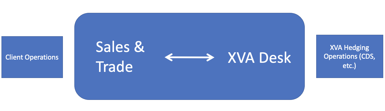
Figure 1: A XVA Trading Desk (adapted from [31])

The role of the XVA desk in a trading operation is outlined in the Figure 1. The XVA desks play a primary role of valuing these adjustments, and writes protection against losses of the derivative trading operations. They might also optionally warehouse this risks or hedge against these risks. In our discussion, we narrowed the scope of the XVA problem to just credit risks, which are risk that a party binded by a financial contract fails to make due payments to the other party. Credit Valuation Adjustment (CVA), can then be defined as the market price of a credit risk on a financial instrument as a portfolio of instruments that are marked to market. In particular,

$$\rm{CVA}=V(\rm{DefaultRiskFree})-V(\rm{DefaultRisky}).$$

This valuation adjustment is synonymous with how a chronic smoker might have to pay higher premiums on insurance. Since the credit crises of 2007, the Basel Framework recommends a bilateral model, but many banks to this day use unilateral CVA and the use of bilateral models remain contentious [15]. In this paper we only consider the unilateral credit adjustments, which do not take into account one’s own default risk and hence simpler to calculate. To that effect, the CVA formula in our discussion is strictly positive.

While there is no market standard, there are two types of CVAs - unilateral CVA and bilateral CVA [8]. The difference is that unilateral CVA only takes into consideration the counterparty credit risk while bilateral CVA also takes into account the credit risk of ‘self’, or the accounting party. Many derivative contracts such as interest rate swaps involve cash flow payments in both direction based on market conditions and as such, both parties carry the risk.

A.1 Derivation of the CVA Formula

The mathematics presented are derivative of previous work, mainly [15], with some additive and original intermediate workings provided. Rearranging the CVA equation, we have $V(\rm{DefaultRisky})=V(\rm{DefaultRiskFree})-\rm{CVA}$. As before, we define the terminologies

• ${\hat{V}}$: economic value of a basket of derivatives

• $V_{t}$: BSM value of a basket of derivatives at time t

• $V_{t}^{+}$: positive components of a basket of derivatives at time t

• $V_{t}^{-}$: negative components of a basket of derivatives at time t

• $C(t,T)$: cash flows for a portfolio of trades from time t to T

Recall that the portfolio process is adapted to filtration $\mathcal{F}_{t}$. By definition,

$$\hat{V}_{t,\tau}=V(t<\tau)+V_{Recovery}(t\geq\tau)$$ (49)

$$V(t<\tau)=\mathbb{E}\left[C(t,\tau)_{\mathbbm{1}_{\tau<T}}+C(t,T)_{\mathbbm{1}_{\tau\geq T}}|\mathcal{F}_{t}\right]$$ (50)

At time of default, $V_{Recovery}(\tau)=R(V_{\tau})^{+}+(V_{\tau})^{-}$ and the adjusted value of the portfolio at time $t$ assuming default at $\tau$ is expressed [15]:

$$\hat{V}_{t,\tau}=\mathbb{E}[C(t,\tau)_{\mathbbm{1}_{\tau<T}}+C(t,T)_{\mathbbm{1}_{\tau\geq T}}+\mathbb{E}[(R(V_{\tau})^{+}+(V_{\tau})^{-})_{\mathbbm{1}_{\tau<T}}|\mathcal{F}_{t}]|\mathcal{F}_{t}]$$ (51)

By Linearity of Expectations, Tower Property and using $V_{t}=(V_{t})^{+}+(V_{t})^{-}$:

$$\hat{V}_{t,\tau}=\mathbb{E}[C(t,\tau)_{\mathbbm{1}_{\tau<T}}|\mathcal{F}_{t}]+\mathbb{E}[C(t,T)_{\mathbbm{1}_{\tau\geq T}}|\mathcal{F}_{t}]+\mathbb{E}\left[\mathbb{E}\left[(R(V_{\tau})^{+}+(V_{\tau})^{-})_{\mathbbm{1}_{\tau<T}}|\mathcal{F}_{t}\right]|\mathcal{F}_{t}\right]$$ (52)

$$=\mathbb{E}[C(t,\tau)_{\mathbbm{1}_{\tau<T}}|\mathcal{F}_{t}]+\mathbb{E}[C(t,T)_{\mathbbm{1}_{\tau\geq T}}|\mathcal{F}_{t}]+\mathbb{E}[(R(V_{\tau})^{+}+(V_{\tau})^{-})_{\mathbbm{1}_{\tau<T}}|\mathcal{F}_{t}]$$ (53)

$$=\mathbb{E}[C(t,\tau)_{\mathbbm{1}_{\tau<T}}|\mathcal{F}_{t}]+\mathbb{E}[C(t,T)_{\mathbbm{1}_{\tau\geq T}}|\mathcal{F}_{t}]+\mathbb{E}[R(V_{\tau})^{+}_{\mathbbm{1}_{\tau<T}}|\mathcal{F}_{t}]+\mathbb{E}[(V_{\tau})^{-}_{\mathbbm{1}_{\tau<T}}|\mathcal{F}_{t}]$$ (54)

$$=\mathbb{E}[C(t,\tau)_{\mathbbm{1}_{\tau<T}}|\mathcal{F}_{t}]+\mathbb{E}[C(t,T)_{\mathbbm{1}_{\tau\geq T}}|\mathcal{F}_{t}]+\mathbb{E}[R(V_{\tau})^{+}_{\mathbbm{1}_{\tau<T}}|\mathcal{F}_{t}]+\mathbb{E}[((V_{\tau}-(V_{\tau})^{+})_{\mathbbm{1}_{\tau<T}}|\mathcal{F}_{t}]$$ (55)

$$=\mathbb{E}[C(t,\tau)_{\mathbbm{1}_{\tau<T}}|\mathcal{F}_{t}]+\mathbb{E}[C(t,T)_{\mathbbm{1}_{\tau\geq T}}|\mathcal{F}_{t}]-\mathbb{E}[(1-R)*(V_{\tau})^{+}_{\mathbbm{1}_{\tau<T}}|\mathcal{F}_{t}]+\mathbb{E}[V_{\tau\mathbbm{1}_{\tau<T}}|\mathcal{F}_{t}].$$ (56)

Note that by definition, the value of a portfolio is just the sum of its discounted future cash flows. $V_{t}=\mathbb{E}[C(t,T)|\mathcal{F}_{t}]$, and the equation above can be simplified:

$$\hat{V}_{t,\tau} = \mathbb{E}[C(t,\tau)_{\mathbbm{1}_{\tau<T}}|\mathcal{F}_{t}]+\mathbb{E}[C(t,T)_{\mathbbm{1}_{\tau\geq T}}|\mathcal{F}_{t}]-\mathbb{E}[(1-R)*(V_{\tau})^{+}_{\mathbbm{1}_{\tau<T}}|\mathcal{F}_{t}]$$ (58)

$$+\ \mathbb{E}[\mathbb{E}[(C(\tau,T)_{\mathbbm{1}_{\tau<T}}|\mathcal{F}_{t}]]|\mathcal{F}_{t}]$$

$$= \mathbb{E}[C(t,\tau)_{\mathbbm{1}_{\tau<T}}|\mathcal{F}_{t}]+\mathbb{E}[C(t,T)_{\mathbbm{1}_{\tau\geq T}}|\mathcal{F}_{t}]-\mathbb{E}[(1-R)*(V_{\tau})^{+}_{\mathbbm{1}_{\tau<T}}|\mathcal{F}_{t}]$$

$$+\mathbb{E}[C(\tau,T)_{\mathbbm{1}_{\tau<T}}|\mathcal{F}_{t}]$$

$$= \mathbb{E}[(C(t,\tau)+C(\tau,T))_{\mathbbm{1}_{\tau<T}}|\mathcal{F}_{t}]+\mathbb{E}[C(t,T)_{\mathbbm{1}_{\tau\geq T}}|\mathcal{F}_{t}]$$ (61)

$$-\ \mathbb{E}[(1-R)*(V_{\tau})^{+}_{\mathbbm{1}_{\tau<T}}|\mathcal{F}_{t}]$$

$$= \mathbb{E}[C(t,T)_{\mathbbm{1}_{\tau<T}}|\mathcal{F}_{t}]+\mathbb{E}[C(t,T)_{\mathbbm{1}_{\tau\geq T}}|\mathcal{F}_{t}]-\mathbb{E}[(1-R)*(V_{\tau})^{+}_{\mathbbm{1}_{\tau<T}}|\mathcal{F}_{t}]$$ (62)

$$= ({\mathbbm{1}_{\tau<T}}+{\mathbbm{1}_{\tau\geq T}})\mathbb{E}[C(t,T)|\mathcal{F}_{t}]-\mathbb{E}[(1-R)*(V_{\tau})^{+}_{\mathbbm{1}_{\tau<T}}|\mathcal{F}_{t}]$$ (63)

$$= \mathbb{E}[C(t,T)|\mathcal{F}_{t}]-\mathbb{E}[(1-R)*(V_{\tau})^{+}_{\mathbbm{1}_{\tau<T}}|\mathcal{F}_{t}]$$ (64)

$$= V_{t}-\mathbb{E}[(1-R)*(V_{\tau})^{+}_{\mathbbm{1}_{\tau<T}}|\mathcal{F}_{t}].$$ (65)

Hence, we obtain $\rm{CVA}(t)=\mathbb{E}[(1-R)(V_{\tau})^{+}|\mathcal{F}_{t}]$. Assume deterministic Loss Given Defaults, as well as the independence of credit risk to market factors of the BSM model, such that $\mathcal{F}_{t}=\mathcal{G}_{t}\cup\mathcal{H}_{t}$, where $V_{t}$ is adapted to the filtration $\mathcal{G}_{t}\subseteq\mathcal{F}_{t}$. Then, by the Tower Property:

$$CVA(t) = \mathbb{E}\left[\mathbb{E}\left[(1-R)\left(V_{\tau}\right)^{+}|\mathcal{G}_{t}\right]|\mathcal{F}_{t}\right]=\mathbb{E}[g_{\mathcal{G}_{t}}(\tau)|\mathcal{F}_{t}]$$ (66)

$$= \int^{T}_{\tau=t}f_{\tau|\mathcal{F}_{t}}(\tau)g_{\mathcal{G}_{t}}(\tau)d\tau$$ (67)

$$= \int^{T}_{\tau=t}f_{\tau|\mathcal{F}_{t}}(\tau)\mathbb{E}[(1-R)(V_{\tau})^{+}|\mathcal{G}_{t}]d\tau$$ (68)

$$= (1-R)\int^{T}_{\tau=t}f_{\tau|\mathcal{F}_{t}}(\tau)\mathbb{E}[(V_{\tau})^{+}|\mathcal{G}_{t}]d\tau$$ (69)

$$\overset{\lim_{n\to\infty}}{=} (1-R)\sum^{n-1}_{i=0}\phi(\tau\in(t_{i},t_{i+1}])\mathbb{E}[(V_{t_{i}})^{+}|\mathcal{G}_{t}].$$ (70)

Appendix B Problems in Quantitative Finance

B.1 Introduction to Credit Curve Bootstrapping

The CVA formula was observed to be a linear combination in weights of expected exposure profiles, with the weights being defined by probability distributions of the default time $\tau$. In practise, these survival probabilities are taken from historical data or derived from implied Credit Default Swap (CDS) spreads using the risk-neutral measure.

The standard market practise is to derive them from the CDS spreads [15]. We outline the process for obtaining default probabilities from market data, and refer to a more detailed treatment by Castellacci [9]. We assume that the credit market for the derivatives in our portfolio are liquid; that CDS are readily traded and their market data is known. We operate under the settings of the ‘JPMorgan model’, for which we outline the assumptions below.

Let the survival probability for default time be defined by $S(t)=1-\phi(t)$. The hazard rate corresponding to $\tau$ is defined via the deterministic function [15]:

$$S(t)=\exp\left\{-\int^{t}_{0}h(u)du\right\}.$$ (71)

By extension of the deterministic hazard rate process, it follows that hazard rates are independent of the other market variables under discussion, such as the discount factor. The credit default swap derivative is a financial instrument that allows market participants to offset credit risk. The buyer of a CDS makes payments to the seller until some maturity date $T$. In return, the seller agrees that in the event that the reference entity defaults, the seller has to payout a sum as a percentage of the insured notional value.

These payments that the buyer of a CDS pays is in the form of a spread, which is a percentage of the notional value paid out to the seller per annum. The trade value is characterized by two different ‘legs’, known as the floating and the fixed leg. In a liquid market, the observables are these spreads at different maturities, and it is this curve representing spreads as a function of time that is coined as the term structure. Heuristically, we might expect that higher spreads are coincident with higher probabilities of default, since the rational seller/insurer shall demand higher premiums on insuring more risky reference securities. The default probabilities are said to be ‘implied’ by the observed term structure of spreads. Our objective is to estimate these survival probabilities implied, where maturities of different length imply different risk expectations with respect to time.

Under the assumptions that the hazard rate is a piecewise constant, we may partition the time axis up to maturity such that $0=T_{0}\leq T_{1}\cdots\leq T_{n}=T$, where for $t\in[T_{i-1},T_{i})$, $h(t)=h_{i}\in\mathbb{R}$.

The survival probabilities are expressed [9]:

$$S(t)=\exp\left\{-\sum^{n(t)}_{i=1}h_{i}\Delta T_{i}+h_{n(t)+1}(t-T_{n(t)})\right\},$$ (72)

where $n(t)=\max\{i\leq n:T_{i}\leq t\}$ and $\Delta T_{i}=T_{i}-T_{i-1}$.

The JPMorgan model makes certain key assumptions outlined:

1. Hazard rates are piecewise constant between different maturities.

2. Default process independent of the interest rate process.

3. Default leg pays at the end of each accrual period.

4. Occurrence of default is midway during each payment period.

5. Accrual payment is made at the end of each period.

Under these assumptions, we may attempt to value the legs at $T_{0}$ maturing at $T$. The present value of the fixed leg can be denoted

$$V_{fix}(T)=s\sum^{n}_{i=1}\alpha_{i}Z(0,T_{i})\left(S(T_{i})+\frac{1}{2}(S(T_{i-1})-S(T_{i}))\right),$$ (73)

and the present value of the floating leg to be

$$V_{float}(T)=(1-R)\sum^{n}_{i=1}Z(0,T_{i})\left(S(T_{i-1})-S(T_{i})\right),$$ (74)

where $\alpha_{i}$ is the day count fraction between premium dates corresponding to the period between $T_{i-1}$ and $T_{i}$ of a chosen convention, and $Z(0,T_{i})$ is the value of a risk-free zero coupon bond starting from $T_{0}$ and maturing at $T_{i}$. If we assume a constant risk-free interest rate $r\in(0,1)$, then $Z(0,T_{i})=\exp\{-rT_{i}\}$. Otherwise, we may calibrate it to the interest rate term structure.

Note that a fair contractual agreement between the buyer and the seller at inception is such that $V_{fix}(t)=V_{float}(t)$ for all $t$. Note that the value of the contract at the onset must be zero, since the agreement is fair. In particular, let the value of the CDS contracts at time $t$ be denoted $C(t)$, then for all $t$, $V_{float}(t)-V_{fix}(t)=0$. Assuming that the market data/spreads obtained are $s_{1},s_{2}\cdots s_{m}$ corresponding to maturities $T_{n_{1}},T_{n_{2}}\cdots T_{n_{m}}$, we have $0\overset{!}{=}C(T_{n_{1}})=$

$$(1-R)\sum^{n_{1}}_{i=1}Z(0,T_{i})\left(S(T_{i-1})-S(T_{i})\right)-s_{1}\sum^{n_{1}}_{i=1}\alpha_{i}Z(0,T_{i})\left(S(T_{i})+\frac{1}{2}(S(T_{i-1})-S(T_{i}))\right).$$ (75)

Note that in the equation above, $R$ is a deterministic, known recovery rate, $Z(0,T_{i})$ can be derived via calibrating the interest rate term structure, and $\alpha_{i}$ is also known. The only unknown variable is the survival probabilities which are a function of the hazard rates. In fact, the Equation (75) is an implicit equation on $h_{1}$ and may be solved via numerical solvers.

Repeating for the next maturity, we have $0\overset{!}{=}C(T_{n_{2}})=$

$$(1-R)\sum^{n_{2}}_{i=1}Z(0,T_{i})\left(S(T_{i-1})-S(T_{i})\right)-s_{1}\sum^{n_{2}}_{i=1}\alpha_{i}Z(0,T_{i})\left(S(T_{i})+\frac{1}{2}(S(T_{i-1})-S(T_{i}))\right),$$ (76)

which is an implicit equation in $h_{1}$ and $h_{2}$. Using the result from approximation of $h_{1}$, we may use equivalent methods to derive $h_{2}$. These steps may be iterated up to $T_{n_{m}}$, and the survival probabilities be determined via Equation (71) vis-a-vis the hazard rates. The cumulative distribution function $\phi(t)$ immediately follows by taking the complement of $S(t)$.

B.2 Introduction to Discounting and Interest Rate Term Structure

In our discussion, we have assumed access to oracles that give discounted values of the portfolio. In the Financial Preliminary, we introduced the concept of discounting, which is necessary to obtain the present value of future valuations of a portfolio. In particular, $V_{t}=\exp\{-\int^{t}_{0}r_{u}du\}V^{\prime}_{t}$. Note that we may relax this assumption and let the short rate take negative values, as is often observed in modern sovereign rates. A simple modelling choice would be to choose a deterministic discount factor $r_{t}=r$ calibrated to historical data. We may also model interest rates as stochastic processes evolving over time. Broadly speaking, interest rate models fall into the 4 categories - short rate models, Heath-Jarrow-Morton (HJM) models, Market Models and Markov Functional Models. In the context of XVA calculations, we are most concerned with the efficiency of their computation within the Monte Carlo simulation; and hence we prefer Markovian models over non-Markovian interest rate models in practise [15]. Markovian models have the advantage that they may be pre-computed in the initialization stage and then cached for use when the Monte Carlo paths are generated. We give an overview of the discussion of such a model, called the Extended-Vasicek model under the settings of a Heath-Jarrow-Morton (HJM) framework.

The interest rate term structure may be described via the forward rates $f(t,T,T+\Delta)$, which is the interest rate for borrowing agreed to at time $t$, to borrow from time $T$ to $T+\Delta$. The instantaneous forward rate is the forward rate as the limit of $\Delta\to 0$, and we denote it as $f(t,T)$. The market observables relating to the term structure are these instantaneous forwards at different starting times $t_{i}$ with different durations $T-t_{i}$. The short rates $r(t)$ may be defined in terms of the instantaneous forwards; it is the rate agreed to borrow when $T-t_{i}$ goes to zero, such that $r(t)=f(t,t)$.

Here we introduce the concept of the zero coupon bond (ZCB), which is an asset that pays a dollar at maturity $T$ and pays no coupons. Denote the value of such an instrument evaluated at $t$ maturing at $T$ as $Z(t,T)$. By definition, $Z(T,T)=1$. Under the principle of no arbitrage, $Z(t,T)=\exp\{-y(T-T)(T-t)\}$, where $-y(T-t)$ is the interest rate of borrowing from $t$ to $T$. Since we shall be indifferent between agreeing to borrowing at discrete intervals between $t$ and $T$ and agreeing to borrow in one contract, the value of the ZCB can be expressed in terms of the forward rates. That is:

$$Z(t,T) = \exp\left\{-\sum^{n-1}_{i=0}f(t,t_{i})\Delta t_{i}\right\}$$ (77)

$$\overset{\lim_{n\to\infty}}{=} \exp\left\{-\int^{T}_{t}f(t,u)du\right\}$$ (78)

The opposite of the ZCB is the money market account, or the bank account. Previously, we argued that the bank account at time $t$ has value $B_{t}=B_{0}\exp\{rt\}$, where $B_{0}$ is the initial sum invested. However, treating interest rates as a stochastic process, we may more generally express it under the short rates:

$$B_{t}=B_{0}\exp\left\{\int^{t}_{0}r(u)du\right\}.$$ (79)

We have obtained the bank account in terms of the stochastic short rates which are random and which shall be analysed under the risk-neutral probability measures. Recall that the Fundamental Theorem of Asset Pricing states that discounted asset prices are martingales under the risk-neutral measure $\mathbbm{Q}$. In particular, the ZCB scaled by the bank account is a martingale. Using the definitions of the bank account in Equation (79) and that $Z(T,T)=1$, we have:

$$\frac{Z(t,T)}{B_{t}}=\mathbb{E}_{\mathbb{Q}}\left[\frac{Z(T,T)}{B_{T}}|\mathcal{F}_{t}\right]\to Z(t,T)=\mathbb{E}_{\mathbb{Q}}\left[\exp\left\{-\int^{T}_{t}r(u)du\right\}\ |\mathcal{F}_{t}\right].$$ (80)

Note that by definition, $Z(t,T+\Delta)=Z(t,T)\exp\{-f(t,T,T+\Delta)\Delta\}$. We may express the instantaneous forwards in terms of the ZCB dynamics [7]:

$$f(t,T)=-\frac{\delta}{\delta T}\ln Z(t,T).$$ (81)

The dynamics of the instantaneous forwards under HJM framework are stated [15]:

$$df(t,T)=\mu(t,T)dt+\sigma_{f}(t,T)dW(t)$$ (82)

where $\mu$ is stochastic drift as a function of time, $\sigma_{f}$ the volatility of the instantaneous forwards, and $W$ is a Brownian motion.

To satisfy the principle of no arbitrage, it can be shown that the stochastic drift has the constraints such that the dynamics of the instantaneous forward $f$ under risk-neutral measure $\mathbbm{Q}$ is [7]:

$$df(t,T)=\left(\sigma_{f}(t,T)\int^{T}_{t}\sigma_{f}(t,u)du\right)dt+\sigma_{f}(t,T)dW_{t}.$$ (83)

An interest rate model that falls under the HJM framework is the Extended-Vasicek model [15], which allows for fitting of the initial term structure by allowing the long term mean reversion level to a function of time. In particular, it models of the dynamics of the short rate as such [7]:

$$dr_{t}=\alpha(\theta_{t}-r_{t})dt+\sigma dW_{t},$$ (84)

where $\theta_{t}$ is the long term mean of the short rates as a function of time, and $\alpha$ is the speed of mean-reversion.

Relating it to the HJM framework and using stochastic calculus techniques [28], it can be shown that the short rate dynamics are equivalent to [15]:

$$dr_{t}=\alpha\left[\frac{1}{\alpha}\frac{\delta f(0,t)}{\delta t}+\frac{\sigma_{f}^{2}}{2\alpha^{2}}(1-\exp\{-2\alpha t\})+f(0,t)-r_{t}\right]dt+\sigma_{f}dW_{t}$$ (85)

The calibration reduces to solving for $\theta_{t}=\frac{1}{\alpha}\frac{\delta f(0,t)}{\delta t}+\frac{\sigma_{f}^{2}}{2\alpha^{2}}(1-\exp\{-2\alpha t\})+f(0,t)$ under a deterministic mean-reversion speed $\alpha$, known $f(0,t)$ and calibrating to ZCB prices implicitly related under the Equation (81) using analytical or numerical solvers.

Similarly, the volatility process may be modelled as stochastic function of time, and calibrated to interest rate option prices such as a strip of co-terminal European swaptions. This is not, however, needed to fit the initial term structure.

References

- [1] Alcazar, J., Cadarso, A., Katabarwa, A., Mauri, M., Peropadre, B., Wang, G., and Cao, Y. Quantum algorithm for credit valuation adjustments. arXiv:2105.12087 (05 2021).
- [2] An, D., Linden, N., Liu, J.-P., Montanaro, A., Shao, C., and Wang, J. Quantum-accelerated multilevel monte carlo methods for stochastic differential equations in mathematical finance. arXiv:2012.06283 (12 2020).
- [3] Azadinamin, A. The bankruptcy of lehman brothers: Causes of failure & recommendations going forward. Social Science Research (2013).
- [4] Black, F., and Scholes, M. The pricing of options and corporate liabilities. Journal of Political Economy 81 (1973), 637–654.
- [5] Bouland, A., van Dam, W., Joorati, H., Kerenidis, I., and Prakash, A. Prospects and challenges of quantum finance. arXiv:2011.06492 (2020).
- [6] Brassard, G., Hoyer, P., Mosca, M., and Tapp, A. Quantum amplitude amplification and estimation. Contemporary Mathematics 305 (2002), 53–74.
- [7] Brigo, D., and Mercurio, F. Interest Rate Models — Theory and Practice: With Smile, Inflation and Credit. 01 2006.
- [8] Brigo, D., Morini, M., and Pallavicini, A. Counterparty Credit Risk, Collateral and Funding: With Pricing Cases For All Asset Classes. 04 2013.
- [9] Castellacci, G. Bootstrapping credit curves from cds spread curves. Social Science Research (11 2008).
- [10] Cont, R., and Tankov, P. Financial modelling with jump processes.
- [11] Cornelissen, A., and Jerbi, S. Quantum algorithms for multivariate monte carlo estimation. arXiv:2107.03410 (2021).
- [12] Doriguello, J. F., Luongo, A., Bao, J., Rebentrost, P., and Santha, M. Quantum algorithm for stochastic optimal stopping problems. arXiv:2111.15332 (2021).
- [13] Dürr, C., and Hoyer, P. A quantum algorithm for finding the minimum. CoRR quant-ph/9607014 (07 1996).
- [14] González Pedraz, C., and Rixtel, A. V. The role of derivatives in market strains during the covid-19 crisis (el papel de los derivados en las tensiones de los mercados durante la crisis del covid-19). Social Science Research (2021).
- [15] Green, A. XVA: Credit, Funding and Capital Valuation Adjustments. John Wiley & Sons, 2015.
- [16] Grover, L. K. A fast quantum mechanical algorithm for database search. In Proceedings of the twenty-eighth annual ACM symposium on Theory of computing (1996), ACM, pp. 212–219.
- [17] Heinrich, S. Quantum summation with an application to integration. Journal of Complexity (2001).
- [18] Hull, J. Options, Futures, and Other Derivatives. Pearson, 2015.
- [19] ISDA. 2003 ISDA Credit Derivatives Definitions. International Swaps and Derivatives Association, 2003.
- [20] Jerrum, M. R., Valiant, L. G., and Vazirani, V. V. Random generation of combinatorial structures from a uniform distribution. Theoretical Computer Science 43 (1986), 169–188.
- [21] Merton, R. C. Theory of rational option pricing. The Bell Journal of Economics and Management Science 4, 1 (1973), 141–183.
- [22] Montanaro, A. Quantum speedup of monte carlo methods. Proc. R. Soc. A 471 (2015), 0301.
- [23] Nielsen, M. A., and Chuang, I. L. Quantum Computation and Quantum Information. Cambridge University Press, 2010.
- [24] Rebentrost, P., Gupt, B., and Bromley, T. R. Quantum computational finance: Monte carlo pricing of financial derivatives. Phys. Rev. A 98 (2018), 022321.
- [25] Rebentrost, P., Santha, M., and Yang, S. Quantum alphatron. arXiv preprint arXiv:2108.11670 (2021).
- [26] She, J.-H., and Grecu, D. Neural network for cva: Learning future values. arXiv:1811.08726 (2018).
- [27] Shor, P. Polynomial-time algorithms for prime factorization and discrete logarithms on a quantum computer. SIAM Review 41, 2 (1999), 303–332.
- [28] Shreve, S. Stochastic Calculus for Finance II: Continuous-Time Models. Springer-Verlag, 2004.
- [29] Stankovska, A. Global derivatives market. SEEU Review 12, 1 (05 2017), 81–93.
- [30] Tang, E. A quantum-inspired classical algorithm for recommendation systems. Electronic Colloquium on Computational Complexity 128 (2018).
- [31] Zeitsch, P. The economics of xva trading. Journal of Mathematical Finance 07 (01 2017), 239–374.
- [32] Zhu, Q., Loeper, G., Chen, W., and Langrené, N. Markovian approximation of the rough bergomi model for monte carlo option pricing. Mathematics 9, 5 (03 2021), 528.