Computing unsatisfiable cores for LTLf specifications
Abstract
Linear-time temporal logic on finite traces (LTLf) is rapidly becoming a de-facto standard to produce specifications in many application domains (e.g., planning, business process management, run-time monitoring, reactive synthesis). Several studies approached the respective satisfiability problem. In this paper, we investigate the problem of extracting the unsatisfiable core in LTLf specifications. We provide four algorithms for extracting an unsatisfiable core leveraging the adaptation of state-of-the-art approaches to LTLf satisfiability checking. We implement the different approaches within the respective tools and carry out an experimental evaluation on a set of reference benchmarks, restricting to the unsatisfiable ones. The results show the feasibility, effectiveness, and complementarities of the different algorithms and tools.
1 Introduction
A growing body of literature evidences the adoption of linear-time temporal logic on finite traces (LTLf) (De Giacomo \BBA Vardi, \APACyear2013) to produce systems specifications (De Giacomo, De Masellis\BCBL \BBA Montali, \APACyear2014). Its widespread use spans across several application domains, including business process management (BPM) for declarative process modeling (Montali \BOthers., \APACyear2010; De Giacomo, De Masellis, Grasso\BCBL \BOthers., \APACyear2014) and mining (Cecconi \BOthers., \APACyear2018; Räim \BOthers., \APACyear2014), run-time monitoring and verification (De Giacomo, De Masellis, Grasso\BCBL \BOthers., \APACyear2014; De Giacomo \BOthers., \APACyear2020; Bauer \BOthers., \APACyear2010), and AI planning (Calvanese \BOthers., \APACyear2002; Sohrabi \BOthers., \APACyear2011; Camacho \BOthers., \APACyear2018; Camacho \BBA McIlraith, \APACyear2019).
When it comes to verification techniques and tool support for LTLf, several studies approach the LTLf satisfiability problem via reduction to LTL (Pnueli, \APACyear1977) satisfiability on infinite traces (De Giacomo, De Masellis\BCBL \BBA Montali, \APACyear2014), or via specific propositional satisfiability approaches (Fionda \BBA Greco, \APACyear2018; Li \BOthers., \APACyear2020). However, no efforts have been devoted thus far to the identification of the formulas that lead to unsatisfiability in LTLf specifications, with the consequence that no support has been offered for modelers and system designers to single out the causes of possible inconsistencies.
In this paper, we tackle the challenge of extracting unsatisfiable cores () from LTLf specifications. Investigating this problem is interesting both from practical and theoretical viewpoints. On the practical side, if unsatisfiability signals that a specification is defective, the identification of unsatisfiable cores provides the users with the opportunity to isolate the source of inconsistency and leads them to a consequent debugging. Notice that determining a reason for unsatisfiability without automated support may reveal unfeasible for a number of reasons that range from the sheer size of the formula to the lack of time and skills of the user (Schuppan, \APACyear2012, \APACyear2018). On the theoretical side, we remark that dealing with the extraction of in LTLf specifications is far from trivial. Indeed, there is neither a default pathway to move from the support provided for LTL to the one that has to be provided for LTLf nor a default algorithm upon which this transition could be based. Concerning the pathway, there are two clear alternatives to address this problem: the first one extends techniques for the extraction of in LTL to the case of LTLf; the second one exploits algorithms that directly compute satisfiability in LTLf to provide support for the extraction of . Concerning the specific algorithms from which to start, the two approaches present different scenarios. In the first pathway, it is easy to observe that several techniques for the extraction of in LTL exist, and could be extended to the case of LTLf. Since recent works show that a single universal best algorithm does not exist and often the systems exhibit behaviors that complement each other (Li \BOthers., \APACyear2019, \APACyear2020), choosing a single algorithm from which to start is less than obvious. In the second pathway, instead, the number of works on satisfiability in LTLf is still rather limited.
In this work, we explore both the above pathways. For the LTL pathway, in particular, we consider algorithms belonging to two reference approaches: one based on model-checking, and the other one based on theorem proving. For the LTLf pathway, we consider a reference state-of-the-art specific reduction to propositional satisfiability. We believe that leveraging reference state-of-the-art approaches provides a rich starting point for the investigation of the problem and the provision of effective tools for the extraction of in LTLf specifications. Our comparative evaluation shows a complementary behavior of the different algorithms.
Our contributions consist of the following:
-
1.
Four algorithms that allow for the computation of an unsatisfiable core through the adaptation of the main reference state-of-the-art approaches for LTL and LTLf satisfiability checking (Section 3). For the LTL pathway, we consider two satisfiability checking algorithms: one based on Binary Decision Diagrams (BDDs) (Clarke \BOthers., \APACyear1997), and the other based on propositional satisfiability (Biere \BOthers., \APACyear2006), and a theorem proving algorithm based on temporal resolution (Hustadt \BBA Konev, \APACyear2003; Schuppan, \APACyear2016). For the native LTLf pathway we consider the reference work of (Li \BOthers., \APACyear2020) based on explicit search and propositional satisfiability. Note that, the techniques based on propositional satisfiability (that is, based on (Biere \BOthers., \APACyear2006) and (Li \BOthers., \APACyear2020)) aim at extracting an , which may not necessarily be the minimum one. The BDD and temporal-resolution based algorithms already allow for the extraction of a minimum unsatisfiable core.
-
2.
An implementation of the proposed four algorithms (Section 4.1). Three implementations extend existing tools for the corresponding original algorithms; the implementation of the algorithm based on temporal resolution, instead, resorts to a pre-processing of the formula to reduce the input to the language restrictions of the original tool.
-
3.
An experimental evaluation on a large set of reference benchmarks taken from (Li \BOthers., \APACyear2020), restricted to the unsatisfiable ones (Sections 4.2 and 4.3). The results show an overall better time efficiency of the algorithm based on the native LTLf pathway (Li \BOthers., \APACyear2020). However, the cardinality of the extracted by the fastest approach is the smallest one in only about half of the cases. The experimental findings exhibit a complementarity of the proposed approaches on different specifications: depending on the varying number of propositional variables, number of conjuncts and degree of nesting of the temporal operators in the benchmarks, it is not rare that some of the implemented techniques achieve a noticeable performance when the other ones terminate with no result and vice-versa.
Since popular usages of LTLf leverage past temporal operators (see e.g., the Declare language (van der Aalst \BOthers., \APACyear2009)), we also provide a way to handle LTLf with past temporal operators (see Definition 2 and all the respective technical parts). This results in the same expressive power as that of pure future version, though allowing for exponentially more succinct specifications (Gabbay, \APACyear1987; Laroussinie \BOthers., \APACyear2002) and more natural encodings of LTLf based modeling languages that make use of these operators. This objective is pursued by leveraging algorithms already supporting LTL with past temporal operators, or through a reduction to LTLf with only future temporal operators to use existing approaches for LTLf satisfiability checking.
2 Background
2.1 LTLf Syntax and Semantics
We assume that a finite set of propositional variables is given.
A state over propositional variables in is a complete assignment of a Boolean value to variables in .
Definition 1.
We say that variable holds in iff is assigned the true value in , and we denote this as .
A finite trace over propositional variables in is a sequence of states. The length of a trace , denoted , is . We denote with the -th state , and with the suffix of the finite trace starting at state , i.e., . An infinite trace over propositional variables in is a sequence of states such that . Given two finite traces and , we indicate with the infinite lazo-shaped trace with prefix and trace repeated indefinitely (intuitively, to indicate that is repeated within an infinite loop).
An LTLf formula is built over the propositional variables in by using the classical Boolean connectives “”, “”, and “”, complemented with the future temporal operators “” (next), “” (weak next), “” (always/globally), “” (eventually/finally), “” (until) and “” (release), and with the past temporal operators “” (yesterday), “” (weak yesterday), “” (historically), “” (once), “” (since), and “” (trigger). The (resp. ) operator is similar to () and solely differs in the way the final (resp. initial) state is dealt with: In the last (resp. initial) state, () is false, while (resp. ) is true. The grammar for building LTLf formulas is:
| Future temporal operators | |||
| Past temporal operators | |||
where is a propositional variable, and are LTLf formulas. Classical implication and equivalence connectives can be obtained in standard ways in terms of the connectives.
Definition 2.
Given a finite trace , the LTLf formula is true in at state s.t. , denoted with , iff:
-
•
iff ;
-
•
iff and ;
-
•
iff or ;
Future temporal operators:
-
•
iff and ;
-
•
iff and , or ;
-
•
iff such that ;
-
•
iff it holds ;
-
•
iff such that and it holds that ;
-
•
iff it holds that , or such that and it holds that ;
Past temporal operators:
-
•
iff and ;
-
•
iff or ;
-
•
iff such that ;
-
•
iff it holds that ;
-
•
iff such that it holds that ;
-
•
iff such that such that ;
We say that is a model of whenever , and we say that is satisfiable, whenever there exists a such that .
Remark.
Notice that the following equivalences hold: , , and . In the following we leverage these equivalences whenever needed to simplify the presentation and the proofs.
The language of an LTLf formula over the set of is defined as the set . Thus, the satisfiability problem for an LTLf formula can be reduced to checking that .
Let us consider the formula . Trace of length 4 such that , , , satisfies the formula, while of length 4 such that , , , is not a model since but in the next state . On the other hand, the LTLf formula does not hold for both traces: does not satisfy the formula because in the last state and there is no next state; as for , but in the next state , and but that is the last state, so no next state exists.
2.1.1 Unsatisfiable core
Given a set of LTLf formulas (considered in implicit conjunction, i.e. ), such that is not satisfiable, we say that a formula is an unsatisfiable core of iff is unsatisfiable. A minimal unsatisfiable core is such that each LTLf formula for is satisfiable. A minimum unsatisfiable core is a minimal unsatisfiable core with the smallest possible cardinality.
2.2 Checking Satisfiability of an LTLf Formula
Checking the satisfiability of an LTLf formula can be reduced to checking language emptiness of a Nondeterministic Finite state Automaton (NFA) (De Giacomo, De Masellis\BCBL \BBA Montali, \APACyear2014). Alternative approaches for LTLf formulas without past temporal operators (De Giacomo \BBA Vardi, \APACyear2013; De Giacomo, De Masellis\BCBL \BBA Montali, \APACyear2014; Fionda \BBA Greco, \APACyear2018) address this problem by checking the satisfiability of an equi-satisfiable LTL formula over infinite traces111We refer the reader to (Pnueli, \APACyear1977; Tsay \BBA Vardi, \APACyear2021) for the semantics of LTL over infinite traces. leveraging on existing well established techniques (e.g (Clarke \BOthers., \APACyear1997; Biere \BOthers., \APACyear2006)). These approaches proceed as follows: (i) they introduce a new fresh propositional variable used to denote the trace has ended; (ii) they require that eventually holds (i.e., ); (iii) they require that once becomes true, it stays true forever (i.e. ); (iv) they translate the LTLf formula into an LTL formula by means of a translation function that is defined recursively on the structure of the LTLf formula as follows:
Theorem 1 ((De Giacomo, De Masellis\BCBL \BBA Montali, \APACyear2014)).
Any LTLf formula without past temporal operators is satisfiable iff the LTL formula
| (1) |
is satisfiable.
Hereafter, we denote with the equation (1) resulting from applying Theorem 1, i.e., . The resulting LTL formula can then be checked for satisfiability with any state of the art LTL satisfiability checker as discussed in (De Giacomo, De Masellis\BCBL \BBA Montali, \APACyear2014; Li \BOthers., \APACyear2020).
Finally, there are SAT based frameworks for LTLf satisfiability checking like e.g. (Li \BOthers., \APACyear2020), where propositional SAT solving techniques are used to construct a transition system for a given LTLf formula , and LTLf satisfiability checking is reduced to a path search problem over the constructed transition system.
Theorem 2 ((Li \BOthers., \APACyear2020)).
Let be an LTLf formula without past temporal operators. is satisfiable iff there is a final state in .
A final state for is any state satisfying the Boolean formula , where (i) is a new propositional atom to identify the last state of satisfying traces (similarly to (De Giacomo, De Masellis\BCBL \BBA Montali, \APACyear2014)); (ii) is the neXt Normal Form of , an equi-satisfiable formula such that there are no Until/Release sub-formulas in the propositional atoms of , built linearly from ; and (iii) is a propositional formula over the propositional atoms of . This approach uses a conflict driven algorithm, leveraging on propositional unsatisfiable cores, to perform the explicit path-search. We report hereafter some useful definitions.
Definition 3 (Conflict Sequence (Li \BOthers., \APACyear2020)).
Given an LTLf formula , a conflict sequence for the transition system is a finite sequence of sets of states such that:
-
•
The initial state is in for ;
-
•
Every state in is not a final state;
-
•
For every state (), all the one-transition next states of are included in .
We call each a frame, and is the frame level.
For a given conflict sequence , the set (for ) represents a set of states that cannot reach a final state of in up to steps.
Theorem 3 ((Li \BOthers., \APACyear2020)).
The LTLf formula is unsatisfiable iff there is a conflict sequence and an such that .
We refer the reader to (Li \BOthers., \APACyear2020) for further details about the construction of , for the SAT based algorithm to check for the existence of a final state in , and for the correctness and termination of such algorithm.
2.2.1 Symbolic Approaches to Check Language Emptiness for LTL
The standard symbolic approaches to check language emptiness for a given LTL formula (Clarke \BOthers., \APACyear1997) consists in (i) building a Symbolic Non-Deterministic Büchi automaton for the formula ; (ii) compute on this automaton the set of fair states; and (iii) intersect it with the set of initial states. The resulting set, denoted with , is a propositional formula whose models represent all states that are the initial state of some infinite trace that accepts . More precisely, let be a symbolic fair transition system over a set of Boolean variables that encodes the formula as discussed for instance in (Clarke \BOthers., \APACyear1997). In this setting, contains all the propositional variables and the Boolean variables (such that ) needed to encode a symbolic fair transition system representing the Büchi automaton for .222We refer the reader to (Clarke \BOthers., \APACyear1997) for (i) the formal definition of symbolic fair transition system and (ii) the details on a construction of a symbolic fair transition system for a given LTL formula . Let be a set of states of such symbolic fair transition system such that:
-
(A1)
All states in are the starting point of some path accepting ;
-
(A2)
All words accepted by are accepted by some path starting from .
We remark that, this approach is suitable both for BDD based and for SAT based approaches to LTL satisfiability.
2.2.2 Temporal Resolution Approaches for LTL Satisfiability
LTL satisfiability can also be addressed with temporal resolution (Fisher, \APACyear1991; Fisher \BOthers., \APACyear2001). Temporal resolution extends classical propositional resolution with specific inference rules for each temporal operator. Temporal resolution has been implemented in solvers like e.g. trp++ (Hustadt \BBA Konev, \APACyear2003) showing effectiveness in analyzing unsatisfiable LTL formulas (Schuppan \BBA Darmawan, \APACyear2011). We refer the reader to (Fisher, \APACyear1991; Fisher \BOthers., \APACyear2001; Hustadt \BBA Konev, \APACyear2003) for further details. We remark that, in (Schuppan, \APACyear2016), it was showed how the temporal resolution proof graph constructed to prove unsatisfiability of an LTL formula without past temporal operators could be used to compute a minimal unsatisfiable core for the respective LTL formula.
3 Extracting unsat cores for LTLf
We present here how four complementary state-of-the-art algorithms can be leveraged to extract unsatisfiable cores for a given set of LTLf formulas, following two different pathways. The first pathway comprises algorithms that extend approaches originally developed for LTL, either relying on satisfiability checking or on temporal resolution; the second pathway instead extends a reference approach developed for LTLf in a native manner.
3.1 Preliminary results
This section presents three results that enable the use of the different frameworks we will adopt in the two different pathways for LTLf unsat core extraction: (i) the extension of the translation function presented in Section 2 to handle LTLf past temporal operators; (ii) a translation that allows to transform any LTLf formula with past temporal operators in an equi-satisfiable one with only future temporal operators; (iii) the use of an activation variable associated to each LTLf formula in to extract unsatisfiable cores from existing frameworks for LTL/LTLf satisfiability frameworks. The first enables the use of any framework for LTL satisfiability checking that supports both past and future temporal operators. The second enables the use of any framework for LTL/LTLf satisfiability checking that supports only future temporal operators. Finally, the latter enables for obtaining the unsatisfiable cores of leveraging existing LTL/LTLf satisfiability frameworks by building an equi-satisfiable formula with these activation variables and looking at the activation variables that will make such equi-satisfiable formula unsatisfiable.
Extending to handle past temporal operators.
We make the following observation: the semantics for past temporal operators over finite traces coincides with the respective semantics on infinite traces (it refers to the prefix of the path). Thus, we can extend the encoding to handle LTLf past temporal operators as follows:
Basically, for past temporal operators the encoding is propagated recursively to the sub-formulas without modifications on the past operator itself. This extension together with Theorem 1 allows us to prove the following corollary.
Corollary 1.
Any LTLf formula is satisfiable iff the LTL formula
| (2) |
is satisfiable.
This corollary enables the use of any framework for LTL satisfiability checking that supports both past and future temporal operators.
Removing past temporal operators.
Given an LTLf formula with past operators, we can build an equi-satisfiable LTLf formula over only future operators using the function that takes an LTLf formula with past operators, and builds a new formula and a set of formulas as follows:
Intuitively, recursively replaces each sub-formula of with a past temporal operator with a new fresh propositional variable, and accumulates in formulas capturing the semantics of the substituted past temporal sub-formulas (e.g., a kind of monitor). In light of this translation, the following theorem follows.
Theorem 4.
Any LTLf formula is satisfiable if and only if the LTLf formula , where , is satisfiable.
Proof.
The proof is by cases on the structure of the formula. We consider only the and past temporal operators since in all the other cases, the preserves the formula and/or rewrites it leveraging on equivalences of temporal operators w.r.t. these two past operators.
-
•
.
Let’s assume that there exists a path such that and (i.e. such that ). We can construct a new path extending the path to consider a new fresh variable such that for and iff . Thus, , and is such that at it holds by construction, thus .Let’s assume that there exists a path such that and there exists an such that . This path will be such that and iff . Thus, .
-
•
Let’s assume that there exists a path such . This path is such that such that it holds that . We can build a new path extending the path to consider a new fresh variable such that , and iff or . Thus, , and it is such that at it holds that or by construction, and thus .Let’s assume there is a path such that and there exists an such that . This path will be such that such that it holds that , thus .
∎
This result enables the use of any framework for LTL/LTLf satisfiability checking that does not support past temporal operators.
Activation variables.
To compute the unsatisfiable core for a given set of LTLf formulas we proceed as follows. For each LTLf formula we introduce an activation variable , i.e., a fresh propositional variable . We then define the LTLf formula . Let be the set of activation variables, thus the formula is over .
We make the following observation: the satisfiability of is conditioned by the activation variables , and we have the following theorems.
Theorem 5.
Let be a set of LTLf formulas over , be a set of propositional variables such that , and . is unsatisfiable if and only if is unsatisfiable.
Proof.
Let us assume unsatisfiable, this means that is unsatisfiable. Let’s now consider , and let us assume it is satisfiable. This means that there exists a path such that all should be true in the initial state , and as a consequence also that all should be satisfiable by such path , and also that the conjunction of all should be so. However, this contradicts the hypothesis that is unsatisfiable.
Let’s assume being unsatisfiable. This means that for all subset such that each is true and all the other variables in are set to false, the conjunction is unsatisfiable. Let’s consider , and let us assume is satisfiable. This means that there exists a path such that , and also that for all . This contradicts the hypothesis that is unsatisfiable. ∎
Theorem 6.
Let be a subset of . Then the set is an unsatisfiable core for iff the formula is unsatisfiable.
Proof.
The proof is analogous to the proof of Theorem 5. ∎
This theorem allows us to obtain the unsatisfiable cores () of by looking at the activation variables that will make unsatisfiable.
3.2 LTLf Unsatisfiable Core Extraction via Reduction to LTL
This section provides details of how we compute LTLf unsat core extraction via reduction to LTL satisfiability checking over infinite traces and via LTL temporal resolution. The first two algorithms we present leverage two different state-of-the-art techniques for LTL satisfiability checking, namely, (i) Binary Decision Diagrams (BDDs) (Bryant, \APACyear1992) approaches such as e.g., (Clarke \BOthers., \APACyear1997); and (ii) SAT based approaches such as e.g., (Biere \BOthers., \APACyear2006). The third algorithm instead is based on temporal resolution for LTL (Hustadt \BBA Konev, \APACyear2003; Schuppan, \APACyear2016), extended to support past temporal operators.
We leverage Theorem 6 to obtain the unsatisfiable cores () of by looking at the activation variables , with , that will make the formula unsatisfiable. In the following, we show how to obtain using different solving techniques.
3.2.1 BDD based LTLf Unsatisfiable Core Extraction
Given the set of LTLf formulas, we build the formula as discussed in Theorem 5. Then we consider the following LTL formula built leveraging Corollary 1:
| (3) |
The set resulting from applying language emptiness algorithms on (i.e. BDDLTLSAT() in Algorithm 1) is a propositional formula whose models encode all states that are the initial state of some infinite trace that accepts , and it contains both the activation variables and the variables together with the variables needed to encode the symbolic Büchi automaton for .
Theorem 7.
There exists a state and a set such that if and only if is satisfiable.
Proof.
Suppose there exists a state in such that . For (A1) there exists a path starting from satisfying . Since for all . Then the path also satisfies .
Suppose that is satisfiable by some word over the alphabet . We extend to such that . Then satisfies . For (A2) there exists a path starting from satisfying . Then satisfies . ∎
This theorem allows for the extraction from of all possible subsets of the implicants that are consistent or inconsistent. In particular, given the set of states corresponding to the assignments to variables , and , the set can be obtained from by quantifying existentially (projecting) the variables corresponding to and and negating (complementing) the result.
| (4) |
is a propositional formula over variables in where each satisfying assignment corresponds to an unsatisfiable core for .
Corollary 2.
. .
Equation (4) can be easily implemented with BDDs through the respective existential quantification and negation BDD operations (Bryant, \APACyear1992; Cimatti \BOthers., \APACyear2007).
Input: ,
Output: or
Algorithm 1 computes all the unsatisfiable cores for a set of LTLf formulas leveraging the BDD based approach discussed in (Clarke \BOthers., \APACyear1997). It takes in input a rewritten formula , and it returns the empty set () if the formula is satisfiable, otherwise it returns an such that is unsatisfiable. It uses BDDLTLSAT algorithm (Clarke \BOthers., \APACyear1997) to compute . See Section 2.2.1 and (Clarke \BOthers., \APACyear1997) for a more thorough discussion on how the check for language emptiness is performed.
Theorem 8.
Algorithm 1 returns if the set of LTLf formulas is satisfiable, otherwise it computes an such that the is an unsatisfiable core for , and then it returns an .
Proof.
The proof is a direct consequence of Theorem 7 and Corollary 2. Indeed, BDDLTLSAT() computes , i.e. the set of states such that are the starting point of some path satisfying . If is satisfiable, it means that any of its subset will be satisfiable as well, thus any possible assignment to will be such that will be satisfiable, and the set , and thus (line 3 of Algorithm 1) . On the other hand, if is unsatisfiable, Equation 4 extracts the formula over variables such that each satisfying assignment for such formula corresponds to an unsatisfiable core for , and this in turn is an unsatisfiable core for . ∎
3.2.2 SAT based LTLf Unsatisfiable Core Extraction
Determining language emptiness of an LTL formula can also be performed leveraging any off-the-shelf SAT-based bounded model checking technique equipped with completeness check (Biere \BOthers., \APACyear2006; Claessen \BBA Sörensson, \APACyear2012). We observe that, all these approaches can be easily extended to extract an unsatisfiable core from a conjunction of temporal constraints leveraging the ability of propositional SAT solvers to check the satisfiability of a propositional formula under a set of assumptions specified in form of literals , i.e., checking the satisfiability of the formula . If turns out to be unsatisfiable, then the SAT solver can return a subset such that is still unsatisfiable. SAT-based bounded model checking (Biere \BOthers., \APACyear2003) encodes a finite path of length with a propositional formula over the set of variables representing the at each time step from 0 to . To check for completeness, they typically encode the fact that the path cannot be extended with states not yet visited (Biere \BOthers., \APACyear2006). We remark that, in model checking one considers both a transition system (i.e. a model) and a temporal logic formula. However, since we are concerned on satisfiability of LTL formulas only, we consider it the universal model (i.e. if is the set of propositional variables, the initial set of states is , and the transitions relation is equal to ), which corresponds to encode symbolically both the initial set of states, and the transitions relation with .
The approach proceeds as illustrated in Algorithm 2 that takes in input the rewritten formula and computes an unsatisfiable core for a set of LTLf formulas leveraging the bounded model checking encoding defined in (Biere \BOthers., \APACyear2006). It uses a completeness formula that is unsatisfiable iff is unsatisfiable, and a witness formula that is satisfiable iff the LTL formula is satisfiable by a path of length .333We refer the reader to (Biere \BOthers., \APACyear2006) for details on how the and propositional formulas are constructed. For increasing value of , we submit the SAT solver a propositional encoding up to the considered of a path satisfying the formula under the assumption that all the literals in are true in the initial time step (). This is achieved through the call SAT_Assume(EncC(), ) that checks the satisfiability of EncC() under the assumptions that the literals in are true. When this call proves the formula unsatisfiable, it is straightforward to get the corresponding unsatisfiable core from the SAT solver in terms of a subset of the variables in , and we are done with the search. On the other hand, if this call returns SAT, we cannot conclude the LTL formula being unsatisfiable. In this case, we need to check if it is satisfiable, i.e. if there exists a lasso-shaped path of length that satisfies the propositional formula EncP() . This is achieved with the simple call SAT(EncP() ). If such call returns SAT the LTL formula is satisfiable, and we are done. Otherwise, we increase and we iterate.
The Algorithm 2 takes in input the rewritten formula and returns the empty set () if the formula is satisfiable, otherwise it returns a subset such that is unsatisfiable.
Input: ,
Output: or
Lemma 1.
is satisfiable iff there exists a lasso shaped witness such that .
Proof.
Let be a finite path corresponding to a satisfying assignment for . From assumption (A1) such path should be such that s.t. . With and the construction of we conclude that the projection of onto satisfies .
Let us assume a lasso shaped witness for . Any extension to such that is a witness for . As a consequence, is satisfiable. ∎
Lemma 2.
Let , if is unsatisfiable under assumption , then is unsatisfiable.
Proof.
Let be unsatisfiable under assumption . Let’s assume there exists a witness of . We can extend such path to a path over variables such that is a witness for , and this contradicts the assumption (A2). ∎
Theorem 9.
Algorithm 2 returns if the set of LTLf formulas is satisfiable, otherwise it returns an such that the set is an unsatisfiable core for .
The algorithm above uses the (Biere \BOthers., \APACyear2006) encoding for both and . We remark that the schema can also be easily adapted to leverage other algorithms e.g. based on -liveness (Claessen \BBA Sörensson, \APACyear2012) or liveness to safety (Biere \BOthers., \APACyear2002) both relying on the IC3 (Bradley, \APACyear2011) algorithm. What intuitively changes is the propositional encoding of the LTL formula and the calls to the SAT solver to reflect the IC3 algorithm.
3.2.3 Temporal Resolution based LTLf Unsatisfiable Core Extraction
We can extract the unsat core of a set of LTLf formulas via LTL temporal resolution (Hustadt \BBA Konev, \APACyear2003) (TR) leveraging the results previously discussed in this paper and existing LTL temporal resolution engines equipped for temporal unsat core extraction (Schuppan, \APACyear2016). The approach is as follows. First we build the formula . Second, we apply Theorem 4 to remove the past temporal operators. Third, we leverage Theorem 1 to convert the LTLf formula into an equi-satisfiable LTL formula. Finally, the resulting LTL formula is given in input to any LTL temporal resolution solver suitable to extract a temporal unsatisfiable core (e.g. trp++ (Schuppan, \APACyear2016)) by enforcing the activation variables to hold (i.e. enforcing in conjunction with the resulting LTL formula). If the LTL temporal resolution solver responds UNSAT, looking at the activation variables in the extracted temporal unsatisfiable core we get an unsat core of the original set of LTLf formulas.
Input: ,
Output: or
Algorithm 3 computes an unsatisfiable core for a set of LTLf formulas leveraging a LTL temporal resolution prover equipped for extracting an unsatisfiable core like, e.g., TRP++ (Schuppan, \APACyear2016). It takes in input the formula and returns the empty set () if the formula is satisfiable, otherwise it returns a subset such that is unsatisfiable. It uses the TRP++ algorithm (Schuppan, \APACyear2016) to compute the unsatisfiable core , and then it extracts from this only the formulas corresponding to (denoted in the algorithm with ). The TRP++() algorithm discussed in (Schuppan, \APACyear2016) first converts the LTL formula into an equi-satisfiable set of Separated Normal Form (SNF) (Fisher, \APACyear1991) clauses , and then it checks whether this set is satisfiable or not, and in case of unsatisfiability it computes an unsatisfiable core and returns it by applying a reconstruction w.r.t. the original set of LTL formulas. We refer the reader to (Schuppan, \APACyear2016) for the details of the algorithm and for the respective proof of correctness of the TRP++ algorithm.
Theorem 10.
Algorithm 3 returns if the set of LTLf formulas is satisfiable, otherwise it returns an such that the set is an unsatisfiable core for .
Proof.
If the set is satisfiable, then the formula where , is satisfiable since it leverages on transformations that preserve satisfiability (as proved in Theorems 4,1 and 6). Thus also TRP++() returns sat, and the algorithm returns to indicate the formula is satisfiable.
On the other hand, if is unsatisfiable, then also is unsatisfiable. Thus TRP++() returns UNSAT, together with an unsatisfiable core for the formula . We remark that, given the structure of , each will be then converted into an SNF clause which thus will be part of the set of SNF clauses used internally by TRP++. Since this formula is unsatisfiable, the TRP++ algorithm will extract an unsat core such that is unsatisfiable. among other clauses will contain some for that will correspond to the respective formulas in (thanks also to Theorem 6), and thus this set will represent an unsatisfiable core for . ∎
3.3 LTLf Unsatisfiable Core Extraction via Native SAT
We adapted the native SAT based LTLf satisfiability approach discussed in (Li \BOthers., \APACyear2020) to extract the unsatisfiable core. Since the original approach for LTLf satisfiability checking in (Li \BOthers., \APACyear2020) was not supporting past temporal operators, we rely on Theorem 4 to get rid of the past temporal operators obtaining an equi-satisfiable LTLf formula without past temporal operators.
The algorithm originally discussed in (Li \BOthers., \APACyear2020) can be extended to extract the unsat core of a set of LTLf formulas as follows (see Algorithm 4). First, we build the LTLf formula . Then, we apply Theorem 4 to get an equi-satisfiable formula. The resulting formula (without past temporal operators) is then passed in input to the algorithm SATLTLF discussed in (Li \BOthers., \APACyear2020). The SATLTLF algorithm in (Li \BOthers., \APACyear2020) has been modified to enforce that each call to the SAT solver under assumption performed in the algorithm assumes also that the activation variables are all true. We refer the reader to (Li \BOthers., \APACyear2020) for a thorough description of the algorithm (which is out of the scope of this paper). We remark that, the only modifications performed to the algorithm consists in adding the assumptions on the activation variables to the already considered assumptions in each call to satisfiability under assumption already performed within the algorithm itself. Intuitively, the algorithm in (Li \BOthers., \APACyear2020) constructs a conflict sequence (i.e., sequences of states that cannot reach a final state of the transition system constructed from the formula given in input) extracted from the unsat cores resulting from different propositional unsatisfiable queries performed in the algorithm itself. As per Theorem 3 the input LTLf formula is unsatisfiable iff there exists a conflict sequence and an integer such that . When the SATLTLF algorithm returns UNSAT, we extract from the last element of the computed conflict sequence (i.e. ) the unsat core , and the set is an unsat core for leveraging on Theorem 3.
Input: ,
Output: or
Theorem 11.
Algorithm 4 returns if the set of LTLf formulas is satisfiable, otherwise it returns an such that the set is an unsatisfiable core for .
Proof.
If the set is satisfiable, then the formula , where , is also satisfiable since it leverages on transformations that preserve satisfiability (as proved in Theorems 4,1 and 6). Thus leveraging the correctness and completeness of the SATLTLF (Li \BOthers., \APACyear2020), then SATLTLF will report sat, and in turn the Algorithm 4 will report to indicate the set is satisfiable.
On the other hand, if is unsatisfiable, then also the formula will be unsatisfiable. From Theorem 3, then the SATLTLF algorithm will build a conflict sequence and there exists an integer such that , will represent the states such that from there it is not possible to reach a final state for , i.e. there is no path starting from these states that will satisfy , i.e. all the paths from this states will not satisfy .
Thus, for all state there exists a set such that , and the formula will be unsatisfiable, and the set corresponds to an unsat core extracted from by construction of the SATLTLF algorithm (see (Li \BOthers., \APACyear2020) for further details). ∎
3.4 Discussion
We observe that all the described approaches extract one unsat core, though not necessarily a minimum/minimal one. Algorithm 1 could also be easily extended to get the minimal from the set of all possible unsatisfiable cores for the given formula. For the SAT based approaches, a minimum/minimal unsat core could be extracted by leveraging the ability of the SAT solver to get a minimum/minimal propositional unsat core. Similarly, the temporal resolution solver could be instrumented to get a minimum/minimal core. In all cases, it might be possible to get a minimum/minimal one with specialized solvers and/or with additional search. However, this is left for future work.
4 Experimental Evaluation
In this section, we provide details on the implementations of the proposed algorithms (Section 4.1), and then we describe the setup and the data sets used for the experimental evaluation (Section 4.2). We conclude with a report on the results alongside an examination thereof (Section 4.3).
4.1 Implementation of the Algorithms
We implemented Algorithms 1 and 2 as extensions of the NuSMV model checker (Cimatti \BOthers., \APACyear2002) exploiting the built-in support for past temporal operators, the conversion, and Eq. (2). In particular, we enhanced (i) the BDD-based algorithm for LTL language emptiness (Clarke \BOthers., \APACyear1997) and (ii) the SAT-based approaches (Biere \BOthers., \APACyear2006). We shall henceforth refer to these tools as NuSMV-B and NuSMV-S, respectively. The source code for the extended version of NuSMV with these implementations is available at https://github.com/roveri-marco/ltlfuc.
We implemented Algorithm 4 within an extended version of the aaltaf tool (Li \BOthers., \APACyear2020), with a novel dedicated extension to support past temporal operators through . The source code for our extended version of aaltaf is available at https://github.com/roveri-marco/aaltaf-uc.
We implemented Algorithm 3 as a toolchain. First, it calls our variant of aaltaf to generate a file that is suitable for the trp++ temporal resolution solver (Hustadt \BBA Konev, \APACyear2003) using the conversion as per Eq. (2) and . Then, the resulting file is submitted to trp++, and finally the generated is post-processed to extract the auxiliary variables . For the experiments, we used the latest version of trp++ downloadable from http://www.schuppan.de/viktor/trp++uc/.
4.2 The Experimental Setup
Clauses Clauses Family Problems Min. Max. Avg. Family Problems Min. Max. Avg. LTL-as-LTLf/acacia/demo-v3/demo-v3:cl LTL-as-LTLf/anzu/genbuf/genbuf:cl LTL-as-LTLf/alaska/lift/lift LTL-as-LTLf/forobots LTL-as-LTLf/alaska/lift/lift:b LTL-as-LTLf/rozier/counter/counter LTL-as-LTLf/alaska/lift/lift:b:f LTL-as-LTLf/rozier/counter/counterCarry LTL-as-LTLf/alaska/lift/lift:b:f:l LTL-as-LTLf/rozier/counter/counterCarryLinear LTL-as-LTLf/alaska/lift/lift:b:l LTL-as-LTLf/rozier/counter/counterLinear LTL-as-LTLf/alaska/lift/lift:f LTL-as-LTLf/rozier/formulas/n LTL-as-LTLf/alaska/lift/lift:f:l LTL-as-LTLf/schuppan/O1formula LTL-as-LTLf/alaska/lift/lift:l LTL-as-LTLf/schuppan/O2formula LTL-as-LTLf/anzu/amba/amba:c LTL-as-LTLf/schuppan/phltl LTL-as-LTLf/anzu/amba/amba:cl LTLf-specific/benchmarks:ltlf/LTLfRandomConjunction/C100 LTL-as-LTLf/anzu/genbuf/genbuf LTLf-specific/benchmarks:ltlf/LTLfRandomConjunction/V20 LTL-as-LTLf/anzu/genbuf/genbuf:c Overall
For the experimental evaluation, we considered all the unsatisfiable problems reported in (Li \BOthers., \APACyear2020), for a total of problems. To select the specifications of interest to our analysis out of the original testbed, we included only those for which at least one solver declared the set was unsatisfiable and no other tool contradicted the result, as per the experimental data reported by Li et al. To compute the set, we considered all the top-level conjuncts of each formula in the benchmark set. For every benchmark, we used the variant of the formula in the aaltaf format as an input. For the other tools but aaltaf, we implemented within aaltaf dedicated converters to the respective tool input format.
We carried out the experimental evaluation considering the four implementations provided by NuSMV-B, NuSMV-S, our variant of aaltaf, and the trp++ toolchain. We ran all experiments on an Ubuntu 18.04.5 LTS machine, 8-Core Intel(®) Xeon(®) at , equipped with of RAM. We set a memory occupation limit of , and a CPU usage limit of . Additionally, we considered as the maximum depth for NuSMV-S, and we ran NuSMV-B with the BDD dynamic variable reordering mode active (Felt \BOthers., \APACyear1993) to dynamically reduce the size of the BDDs and thus save space over time.444These settings are motivated by similar choices performed in the experimental evaluations carried out in (Cimatti \BOthers., \APACyear2007; Schuppan, \APACyear2016). Whenever the wall-clock timing reported by the implemented technique fell under the lowest sensitivity of the tool (thus being represented as ), we replaced the timing with the minimum non-zero timing reported overall ().
Finally, we have categorized the benchmarking specifications into families, according to their characteristics and provenance. Table 1 shows the number of specifications per family, along with the minimum, maximum and average number of clauses within. In particular, the LTLf-specific/benchmarks/LTLFRandomConjunction/V20 and LTLf-specific/benchmarks/LTLFRandomConjunction/C100 benchmarks are conjunctions of formulas, each selected randomly from standard patterns. They are characterized by a temporal depth (i.e., the maximum nesting of temporal operators) of up to , with propositional variables. The number of conjunctions ranges from to for the former, and from to for the latter. The LTL-as-LTLf/rozier/counter/* benchmarks are characterized by having a small number of propositional variables, and temporal formulas of different temporal depths (from to ). The benchmarks in LTL-as-LTLf/schuppan/O1Formula are characterized by a large number of propositional variables (from to ) with temporal formulas of small depths ( to ) and different operators. The benchmarks in LTL-as-LTLf/schuppan/O2Formula are big conjunctions of formulas of the form with .
All the material to reproduce the experiments reported hereafter is available at https://github.com/roveri-marco/ltlfuc/archive/refs/tags/jair-release-v0.zip.
4.3 The Results
In the experimental evaluation, we considered the following evaluation metrics: (i) the result of the check (expecting all the tools to return unsatisfiability and extract an unsatisfiable core if no resource limit is reached); (ii) the search time to compute and return an unsatisfiable core; (iii) the size of the computed unsatisfiable core. We remark that none of the presented algorithms strives for finding a minimum unsatisfiable core. The approach based on trp++ may be used to that end, and NuSMV-B could in principle be easily adapted to select from the intermediate computed set a minimum unsatisfiable core (as discussed previously). Nevertheless, we pick the first returned for all tools so as to have a fair comparison among them.
 |
 |
| (a) | (b) |
The first result is that, as expected, all the tools reported consistent output when terminating without reaching a resource limit (being it memory, time or search-space depth). In other words, for all the considered benchmarks it was never the case that an algorithm declared the specification as satisfiable. This outcome is in line with the original findings in (Li \BOthers., \APACyear2020). However, we remark that individual algorithms could extract different unsatisfiable cores among the diverse possible ones.
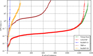
Concerning the computation time, Fig. 1(a) shows the number of problems solved by each algorithm by the timeout on the abscissae and the time taken to solve them cumulatively on the ordinates. Alongside the aforementioned tools, the figure illustrates the performance of the virtual best, that is the minimum time required for each solved instance among the four implementations. Fig. 1(b) is similar to Fig. 1(a), although it excludes the timings for the NuSMV-S runs that reached albeit being unable to prove unsatisfiability (unknown answer) and thus construct an unsatisfiable core. In this figure, then, the virtual best considers only the cases where the tool computed an unsatisfiable core. Both plots show that aaltaf outperforms the other implementations in the majority of cases, although the tail of the virtual-best curve on the right-hand side of both plots exhibits an influence from trp++ and NuSMV-B, thus witnessing complementarity of the proposed approaches. In the remainder of this section, we investigate the comparative assessment more in depth. The overall minimum, maximum, average, and median best timings to return an are , respectively.
 |
|
| (a) | (b) |
 |
|
| (c) | (d) |
 |
|
| (e) | (f) |
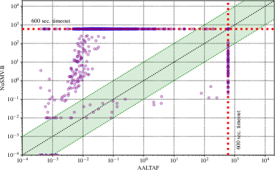
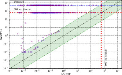
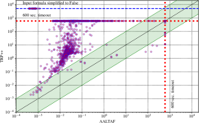
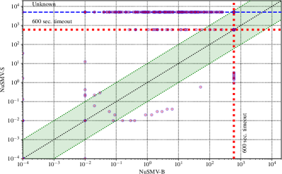
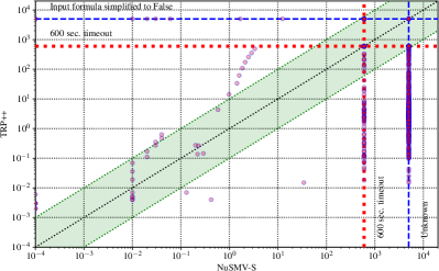
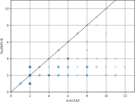
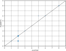
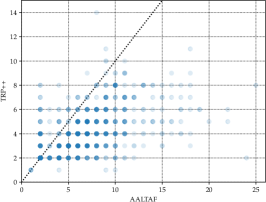
Figure 2 illustrates pairwise comparisons of time efficiency of the considered tools. In particular, Fig. 2(a) compares aaltaf with NuSMV-B, Fig. 2(b) compares aaltaf with NuSMV-S, Fig. 2(c) compares aaltaf with trp++, Fig. 2(d) compares NuSMV-B with NuSMV-S, Fig. 2(e) compares NuSMV-B with trp++, and finally Fig. 2(f) compares NuSMV-S with trp++. Figure 2(c), for instance, shows that aaltaf outperforms trp++: most of the points, indeed, are located above the diagonal, thus indicating that aaltaf requires less time than trp++ to return the unsatisfiable cores. The plot also shows that trp++ exceeds the timeout in several cases (points on the red line marked with “600 sec. timeout”). Furthermore, we observe that trp++ operates a pre-processing phase on the input specification prior to the actual identification of . If it manages to reduce the given set of conjuncts to false at that stage, it stops the computation and raises an alert. The points lying on the line marked with “Input formula simplified to False” indicate those cases. Notice that, this simplification occurred in cases overall, as depicted in Figs. 2(c), (e) and (f). Moreover, NuSMV-B, trp++, NuSMV-S, and aaltaf reached the timeout overall in , , and cases, respectively. NuSMV-S was able to conclude that the formula was unsatisfiable only in cases, and returned an unknown answer (i.e., it reached without being able to decide on unsatisfiability) in cases. We can conclude that, in terms of computation time, aaltaf outperforms the other three tools, NuSMV-B requires less computation time than NuSMV-S and trp++ in the majority of cases, and trp++ reveals slightly faster and less subject to timeouts than NuSMV-S.
|
|
||
|---|---|---|---|
| (a) | (b) |
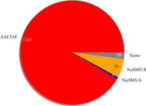
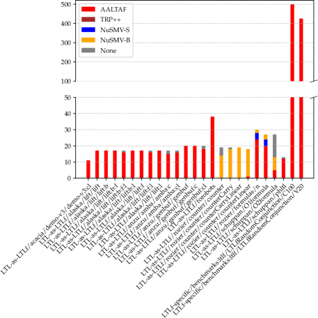
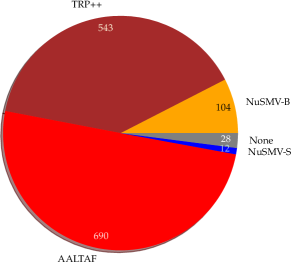
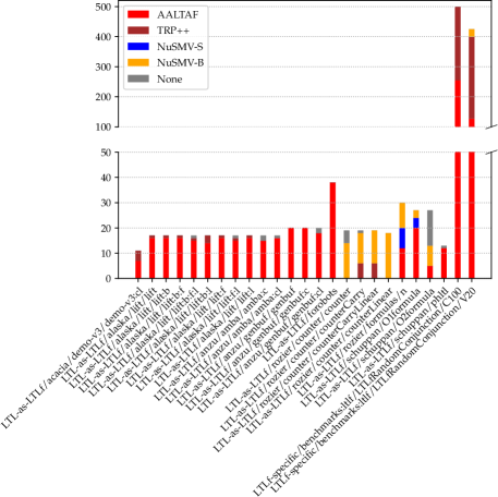
Henceforth, we consider the sole cases in which the tools were able to return an within the given resource limits – thus excluding timeouts, unknown answers and simplifications to false. Figure 3 focuses on computation time: (i) the pie chart in Fig. 3(a) gives an overview of the number of tests in which a tool was the fastest, and (ii) the stacked bar chart in Fig. 3(b) illustrates the results grouped by benchmark family.
The pie chart in Fig. 3(b) confirms that aaltaf is the most time-efficient tool as evidenced by its fastest runs, followed by NuSMV-B (), and NuSMV-S (). In cases, no tool was able to return an unsatisfiable core. As shown by Fig. 3(b), NuSMV-B turned out to find the in minimum time with the LTL-as-LTLf/rozier/counter/*, benchmark families. Moreover, the plot also shows that the problems of the LTL-as-LTLf/schuppan/O2Formula benchmark family are the most challenging ones for all the implemented techniques. Indeed, out of the problems that were not solved by any tools belong to this benchmark family. Moreover, the analysis per benchmark family (see Fig. 3(b)) confirms the superiority in terms of time efficiency of aaltaf in many benchmark families.
 |
 |
|
|
| (a) | (b) | (c) |
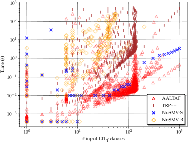
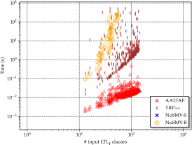
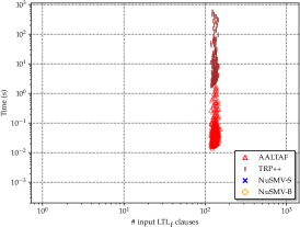
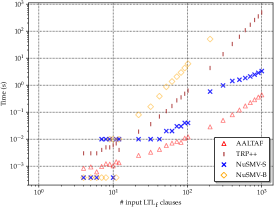
In order to further inspect the correlation between the time performance of the tools and the type of problems solved, we analyzed the relationship between the number of conjuncts of the problems and the corresponding computation time. Figure 4 plots the number of conjuncts in (i.e., its cardinality) against the respective computation time (in seconds) for each of the considered algorithms. Figure 5 isolates the points stemming from three families in particular: LTLf-specific/benchmarks/LTLFRandomConjunction/V20 (Fig. 5(a)), LTLf-specific/benchmarks/LTLFRandomConjunction/C100 (Fig. 5(b)), and LTL-as-LTLf/schuppan/O1Formula (Fig. 5(c)). The plots show that a relationship exists between the number of LTLf clauses and the computation time for all the four tools: the required time overall increases when the number of clauses increases. However, the number of clauses is not the only factor affecting the computation time. For instance, for the LTLf-specific/benchmarks/LTLFRandomConjunction/C100 benchmark family (Fig. 5(b)), the computation time varies independently of the number of conjuncts, which ranges in a short interval ( to clauses, as per Table 1). Also, we can observe that, with this benchmark family, neither NuSMV-S nor NuSMV-B could return an under the imposed experimental resource constraints, while aaltaf appears to be faster than trp++, following the general trend. Figures 5(a) and 5(c) illustrate the different rapidity with which curves increase with the number of conjuncts: the sharpest one is associated to NuSMV-B, followed by trp++ and NuSMV-S (the latter performing better than the former with smaller sets of conjuncts, though, as depicted in Fig. 5(c)). The most gradual upward trend belongs to the curve of aaltaf.
|
|
||
|---|---|---|---|
| (a) | (b) |
As far as the cardinality of the extracted is concerned, Fig. 6 depicts the result of our analysis in the different benchmarks families. As shown in the pie chart of Fig. 6, we report that aaltaf, trp++, NuSMV-B, and NuSMV-S extract that are the smallest in size555Notice that, by “smallest” we mean the unsatisfiable core of smallest cardinality among the ones computed by the solvers. Notice that, the smallest does not necessarily correspond to the minimum one, as discussed when presenting the algorithms. Also, we remark that when two solvers return an of the same size, we associate the best result to the tool that took the lowest time to return it. in , , and cases, respectively. The overall minimum, maximum, average, and median cardinality of the smallest computed were , , , and , respectively.
We observe that for the LTL-as-LTLf/rozier/counter/* benchmarks, NuSMV-B computes the unsatisfiable core with the smallest size in the majority of cases. Notice that, it is also the one that most often performs best in terms of search time (see Fig. 3(b)). NuSMV-B is also able to obtain the smallest with most of the benchmarks within the LTL-as-LTLf/schuppan/O2formula family. On all other benchmarks, aaltaf outperforms the other algorithms, and with the LTLf-specific/* benchmarks, trp++ is the second best solver to find the smallest after aaltaf. These results suggest that NuSMV-B could be preferred on benchmarks with fewer propositional variables and larger temporal depth. However, the SAT based approaches seem to work better on benchmarks with a higher number of propositional variables that are not always directly correlated with one another. Indeed, in these last cases, BDDs may suffer a blow-up in size due to the canonicity of the representation (BDD dynamic variable ordering could help though to a limited extent (Felt \BOthers., \APACyear1993)). Notice that, all solvers were not capable of dealing with most of the the big conjunctions of formulas in LTL-as-LTLf/schuppan/O2Formula (the corresponding tallest stacked bar in Fig. 6 is labeled as “None”, indeed).
 |
|
|
| (a) | (b) | (c) |
 |
|
|
| (d) | (e) | (f) |
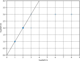
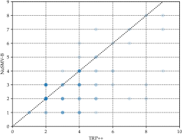
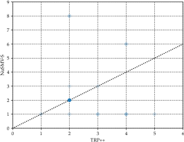
Figure 7 plots the pairwise comparison between different tools on the subset of the cases where both approaches were able to compute the . For instance, Fig.7(a) compares the cardinality of the returned by aaltaf and the cardinality of the returned by NuSMV-B. The plot shows that NuSMV-B are smaller than the ones returned by aaltaf: most of the points are indeed located below the diagonal. The intensity of the points represents the number of cases for which the two algorithms returned with the specific cardinalities corresponding to the coordinates of the point in the plot. Overall, we can observe that when a solution is returned, the cardinality of the returned by trp++ and NuSMV-B is often lower than the cardinality of the returned by aaltaf.
To conclude, we remark that these results (i) evidence an overall better performance of aaltaf both in terms of time efficiency and cardinality of the extracted , and (ii) emphasise a complementarity of the proposed approaches. Table 2 summarizes the findings above. Observe that none of the algorithms outperforms all the others on every benchmark. For example, NuSMV-S and NuSMV-B end up in a timeout and return an unknown answer in considerably many cases, so that a number of problems are solved by only one of them. aaltaf does not always turn out to return the smallest : in a number of cases, trp++, NuSMV-B and NuSMV-S extract of a lower cardinality, excelling in particular in those cases in which aaltaf ends in a timeout. A deeper investigation of the characteristics that lead to such behaviors paves the path for future work.
aaltaf trp++ NuSMV-S NuSMV-B Family Total min.UC min.time min.UC min.time min.UC min.time min.UC min.time None Overall ( %) ( %) ( %) ( %) ( %) ( %) ( %) ( %) ( %) LTL-as-LTLf/acacia/demo-v3/demo-v3:cl ( %) ( %) ( %) LTL-as-LTLf/alaska/lift/lift ( %) ( %) ( %) LTL-as-LTLf/alaska/lift/lift:b ( %) ( %) ( %) LTL-as-LTLf/alaska/lift/lift:b:f ( %) ( %) ( %) LTL-as-LTLf/alaska/lift/lift:b:f:l ( %) ( %) ( %) ( %) LTL-as-LTLf/alaska/lift/lift:b:l ( %) ( %) ( %) LTL-as-LTLf/alaska/lift/lift:f ( %) ( %) ( %) LTL-as-LTLf/alaska/lift/lift:f:l ( %) ( %) ( %) ( %) LTL-as-LTLf/alaska/lift/lift:l ( %) ( %) ( %) LTL-as-LTLf/anzu/amba/amba:c ( %) ( %) ( %) LTL-as-LTLf/anzu/amba/amba:cl ( %) ( %) ( %) LTL-as-LTLf/anzu/genbuf/genbuf ( %) ( %) LTL-as-LTLf/anzu/genbuf/genbuf:c ( %) ( %) LTL-as-LTLf/anzu/genbuf/genbuf:cl ( %) ( %) ( %) LTL-as-LTLf/forobots ( %) ( %) LTL-as-LTLf/rozier/counter/counter ( %) ( %) ( %) LTL-as-LTLf/rozier/counter/counterCarry ( %) ( %) ( %) ( %) LTL-as-LTLf/rozier/counter/counterCarryLinear ( %) ( %) ( %) LTL-as-LTLf/rozier/counter/counterLinear ( %) ( %) ( %) LTL-as-LTLf/rozier/formulas/n ( %) ( %) ( %) ( %) ( %) ( %) LTL-as-LTLf/schuppan/O1formula ( %) ( %) ( %) ( %) ( %) ( %) LTL-as-LTLf/schuppan/O2formula ( %) ( %) ( %) ( %) ( %) LTL-as-LTLf/schuppan/phltl ( %) ( %) ( %) LTLf-specific/benchmarks:ltlf/…/C100 ( %) ( %) ( %) LTLf-specific/benchmarks:ltlf/…/V20 ( %) ( %) ( %) ( %)
5 Related work
To the best of our knowledge, this is the first research endeavour aimed at extrating unsatisfiable cores for LTLf. In the following, we review the most relevant literature concerning LTL/LTLf satisfiability, and LTL SAT-based extraction.
The LTL satisfiability problem has been addressed through tableau-based methods (e.g., (Janssen, \APACyear1999)), temporal resolution (e.g., (Fisher \BOthers., \APACyear2001)), and reduction to model checking (e.g., (Cimatti \BOthers., \APACyear2007; Rozier \BBA Vardi, \APACyear2010, \APACyear2011)). In (Rozier \BBA Vardi, \APACyear2010), a reduction of the LTL satisfiability problem to a model checking problem, and a comparison of different model checkers (explicit/symbolic) has been carried out, resulting in better performance and quality for symbolic approaches. A thorough comparison of the main tools dealing with the LTL satisfiability problem is reported in (Schuppan \BBA Darmawan, \APACyear2011). The paper considers also tableau and temporal resolution based solvers, revealing a complementary behaviour between some of the considered solvers.
The problem of checking the satisfiability of LTLf properties has been the subject of several works (Li \BOthers., \APACyear2014; Fionda \BBA Greco, \APACyear2018; Li \BOthers., \APACyear2020). Li \BOthers. (\APACyear2014), leverage the finite semantics of traces for introducing a propositional SAT based algorithm for the LTLf satisfiability problem together with some heuristics to guide the search. The approach has been implemented in the aalta-finite tool, which has been shown to outperform other existing approaches based on the reduction to the LTL satisfiability problem. This work has been then extended in (Li \BOthers., \APACyear2020) to leverage a transition system (TS) for the input LTLf formula, and reducing satisfiability checking to a SAT based path-search problem over this TS. This approach, also implemented in aalta-finite, has been shown to provide the best results in checking unsatisfiable formulae and comparable results for satisfiable ones. Fionda \BBA Greco (\APACyear2018) investigate the complexity of some fragments of LTLf, and present a SAT based algorithm that outperforms the aalta-finite version in (Li \BOthers., \APACyear2014). Algorithm 3 presented here exploits the work in (Li \BOthers., \APACyear2020) as state-of-the-art tool for checking the satisfiability of LTLf properties.
The extraction for LTL has also been the subject of several studies (Goré \BOthers., \APACyear2013; Awad \BOthers., \APACyear2011; Schuppan, \APACyear2016; Narizzano \BOthers., \APACyear2018). Goré \BOthers. (\APACyear2013) presents a BDD based approach that leverages a method to determine minimal for SAT (Huang, \APACyear2005) to find minimal in LTL. In (Awad \BOthers., \APACyear2011), are extracted by leveraging a tableau-based solver to obtain an initial subset of unsatisfiable LTL formulae and then applying a deletion-based minimization to the subset. The approach, implemented in procmine is part of a tool for the synthesis of business process templates. In (Schuppan, \APACyear2016) fine-grained are extracted constructing and optimizing resolution graphs for temporal resolution. Finally, Narizzano \BOthers. (\APACyear2018) presents a SAT based encoding suitable for the unsat core extraction of LTL-based property specification patterns (Dwyer \BOthers., \APACyear1999) extended with inequality statements on Boolean and numeric variables. Algorithm 4 presented here starts from the work in (Schuppan, \APACyear2016) to compute using temporal resolution.
In the context of process mining, the works in (Di Ciccio \BOthers., \APACyear2017) and (Corea \BBA Delfmann, \APACyear2019) identify inconsistencies for specific LTLf-based constraints contained in the Declare (van der Aalst \BOthers., \APACyear2009) modeling language. They rely on automata language and language inclusion techniques to identify the inconsistencies, and are specific to the precise structure of Declare. Thus they cannot be generalized to address generic LTLf-based specifications.
Finally, works on propositional extraction (e.g., (Huang, \APACyear2005; Marques-Silva \BBA Janota, \APACyear2014; Goldberg \BBA Novikov, \APACyear2003)) could be used to improve the quality of the computed cores but we leave this investigation for future developments.
6 Conclusions and future work
In this paper, we have addressed the problem of LTLf unsatisfiable core extraction, presenting four algorithms based on different state-of-the-art techniques for LTL and LTLf satisfiability checking. We have implemented each of them based on existing tools, and we have carried out an experimental evaluation on a set of reference benchmarks for unsatisfiable temporal formulas. The results have shown feasibility and complementarities of the proposed algorithms.
For future work, we envisage the following research endeavours. We (i) will address the problem of extracting minimal UCs, (ii) plan to extend the approach to other LTL/LTLf algorithms based on -liveness (Claessen \BBA Sörensson, \APACyear2012), liveness to safety (Biere \BOthers., \APACyear2002), or tableau constructions (Geatti \BOthers., \APACyear2021), (iii) intend to extend the problems set with benchmarks from emerging domains (e.g., AI Planning, or BPM), (iv) want to correlate structural information (e.g., cardinality, temporal depth, number of operators) with solving algorithms, (v) aim to investigate the extension to the infinite state case exploiting SMT techniques (Barrett \BOthers., \APACyear2009; Daniel \BOthers., \APACyear2016).
References
- Awad \BOthers. (\APACyear2011) \APACinsertmetastarDBLP:conf/caise/AwadGTW11{APACrefauthors}Awad, A., Goré, R., Thomson, J.\BCBL \BBA Weidlich, M. \APACrefYearMonthDay2011. \BBOQ\APACrefatitleAn Iterative Approach for Business Process Template Synthesis from Compliance Rules An iterative approach for business process template synthesis from compliance rules.\BBCQ \BIn H. Mouratidis \BBA C. Rolland (\BEDS), \APACrefbtitleAdvanced Information Systems Engineering - 23rd International Conference, CAiSE 2011, London, UK, June 20-24, 2011. Proceedings Advanced information systems engineering - 23rd international conference, caise 2011, london, uk, june 20-24, 2011. proceedings (\BVOL 6741, \BPGS 406–421). \APACaddressPublisherSpringer. {APACrefURL} https://doi.org/10.1007/978-3-642-21640-4_31 {APACrefDOI} \doi10.1007/978-3-642-21640-4_31 \PrintBackRefs\CurrentBib
- Barrett \BOthers. (\APACyear2009) \APACinsertmetastarDBLP:series/faia/BarrettSST09{APACrefauthors}Barrett, C\BPBIW., Sebastiani, R., Seshia, S\BPBIA.\BCBL \BBA Tinelli, C. \APACrefYearMonthDay2009. \BBOQ\APACrefatitleSatisfiability Modulo Theories Satisfiability modulo theories.\BBCQ \BIn A. Biere, M. Heule, H. van Maaren\BCBL \BBA T. Walsh (\BEDS), \APACrefbtitleHandbook of Satisfiability Handbook of satisfiability (\BVOL 185, \BPGS 825–885). \APACaddressPublisherIOS Press. {APACrefURL} https://doi.org/10.3233/978-1-58603-929-5-825 {APACrefDOI} \doi10.3233/978-1-58603-929-5-825 \PrintBackRefs\CurrentBib
- Bauer \BOthers. (\APACyear2010) \APACinsertmetastar8133351{APACrefauthors}Bauer, A., Leucker, M.\BCBL \BBA Schallhart, C. \APACrefYearMonthDay2010. \BBOQ\APACrefatitleComparing LTL Semantics for Runtime Verification Comparing ltl semantics for runtime verification.\BBCQ \APACjournalVolNumPagesJournal of Logic and Computation203651-674. {APACrefDOI} \doi10.1093/logcom/exn075 \PrintBackRefs\CurrentBib
- Biere \BOthers. (\APACyear2002) \APACinsertmetastarliveness2safety{APACrefauthors}Biere, A., Artho, C.\BCBL \BBA Schuppan, V. \APACrefYearMonthDay2002. \BBOQ\APACrefatitleLiveness Checking as Safety Checking Liveness checking as safety checking.\BBCQ \APACjournalVolNumPagesElectr. Notes Theor. Comput. Sci.662160–177. {APACrefDOI} \doi10.1016/S1571-0661(04)80410-9 \PrintBackRefs\CurrentBib
- Biere \BOthers. (\APACyear2003) \APACinsertmetastarDBLP:journals/ac/BiereCCSZ03{APACrefauthors}Biere, A., Cimatti, A., Clarke, E\BPBIM., Strichman, O.\BCBL \BBA Zhu, Y. \APACrefYearMonthDay2003. \BBOQ\APACrefatitleBounded model checking Bounded model checking.\BBCQ \APACjournalVolNumPagesAdv. Comput.58117–148. {APACrefURL} https://doi.org/10.1016/S0065-2458(03)58003-2 {APACrefDOI} \doi10.1016/S0065-2458(03)58003-2 \PrintBackRefs\CurrentBib
- Biere \BOthers. (\APACyear2006) \APACinsertmetastarDBLP:journals/lmcs/BiereHJLS06{APACrefauthors}Biere, A., Heljanko, K., Junttila, T\BPBIA., Latvala, T.\BCBL \BBA Schuppan, V. \APACrefYearMonthDay2006. \BBOQ\APACrefatitleLinear Encodings of Bounded LTL Model Checking Linear encodings of bounded LTL model checking.\BBCQ \APACjournalVolNumPagesLog. Methods Comput. Sci.25. {APACrefURL} https://doi.org/10.2168/LMCS-2(5:5)2006 {APACrefDOI} \doi10.2168/LMCS-2(5:5)2006 \PrintBackRefs\CurrentBib
- Bradley (\APACyear2011) \APACinsertmetastarbradley{APACrefauthors}Bradley, A. \APACrefYearMonthDay2011. \BBOQ\APACrefatitleSAT-Based Model Checking without Unrolling SAT-Based Model Checking without Unrolling.\BBCQ \BIn \APACrefbtitleVMCAI Vmcai (\BVOL 6538, \BPG 70-87). \APACaddressPublisherSpringer. \PrintBackRefs\CurrentBib
- Bryant (\APACyear1992) \APACinsertmetastarDBLP:journals/csur/Bryant92{APACrefauthors}Bryant, R\BPBIE. \APACrefYearMonthDay1992. \BBOQ\APACrefatitleSymbolic Boolean Manipulation with Ordered Binary-Decision Diagrams Symbolic boolean manipulation with ordered binary-decision diagrams.\BBCQ \APACjournalVolNumPagesACM Comput. Surv.243293–318. {APACrefURL} https://doi.org/10.1145/136035.136043 {APACrefDOI} \doi10.1145/136035.136043 \PrintBackRefs\CurrentBib
- Calvanese \BOthers. (\APACyear2002) \APACinsertmetastarDBLP:conf/kr/CalvaneseGV02{APACrefauthors}Calvanese, D., De Giacomo, G.\BCBL \BBA Vardi, M\BPBIY. \APACrefYearMonthDay2002. \BBOQ\APACrefatitleReasoning about Actions and Planning in LTL Action Theories Reasoning about actions and planning in LTL action theories.\BBCQ \BIn D. Fensel, F. Giunchiglia, D\BPBIL. McGuinness\BCBL \BBA M. Williams (\BEDS), \APACrefbtitleProceedings of the Eights International Conference on Principles and Knowledge Representation and Reasoning (KR-02), Toulouse, France, April 22-25, 2002 Proceedings of the eights international conference on principles and knowledge representation and reasoning (kr-02), toulouse, france, april 22-25, 2002 (\BPGS 593–602). \APACaddressPublisherMorgan Kaufmann. \PrintBackRefs\CurrentBib
- Camacho \BOthers. (\APACyear2018) \APACinsertmetastarDBLP:conf/aips/CamachoBMM18{APACrefauthors}Camacho, A., Baier, J\BPBIA., Muise, C\BPBIJ.\BCBL \BBA McIlraith, S\BPBIA. \APACrefYearMonthDay2018. \BBOQ\APACrefatitleFinite LTL Synthesis as Planning Finite LTL synthesis as planning.\BBCQ \BIn M. de Weerdt, S. Koenig, G. Röger\BCBL \BBA M\BPBIT\BPBIJ. Spaan (\BEDS), \APACrefbtitleProceedings of the Twenty-Eighth International Conference on Automated Planning and Scheduling, ICAPS 2018, Delft, The Netherlands, June 24-29, 2018 Proceedings of the twenty-eighth international conference on automated planning and scheduling, ICAPS 2018, delft, the netherlands, june 24-29, 2018 (\BPGS 29–38). \APACaddressPublisherAAAI Press. {APACrefURL} https://aaai.org/ocs/index.php/ICAPS/ICAPS18/paper/view/17790 \PrintBackRefs\CurrentBib
- Camacho \BBA McIlraith (\APACyear2019) \APACinsertmetastarDBLP:conf/ijcai/CamachoM19{APACrefauthors}Camacho, A.\BCBT \BBA McIlraith, S\BPBIA. \APACrefYearMonthDay2019. \BBOQ\APACrefatitleStrong Fully Observable Non-Deterministic Planning with LTL and LTLf Goals Strong fully observable non-deterministic planning with LTL and ltlf goals.\BBCQ \BIn S. Kraus (\BED), \APACrefbtitleProceedings of the Twenty-Eighth International Joint Conference on Artificial Intelligence, IJCAI 2019, Macao, China, August 10-16, 2019 Proceedings of the twenty-eighth international joint conference on artificial intelligence, IJCAI 2019, macao, china, august 10-16, 2019 (\BPGS 5523–5531). \APACaddressPublisherijcai.org. {APACrefURL} https://doi.org/10.24963/ijcai.2019/767 {APACrefDOI} \doi10.24963/ijcai.2019/767 \PrintBackRefs\CurrentBib
- Cecconi \BOthers. (\APACyear2018) \APACinsertmetastarDBLP:conf/bpm/CecconiCGM18{APACrefauthors}Cecconi, A., Di Ciccio, C., De Giacomo, G.\BCBL \BBA Mendling, J. \APACrefYearMonthDay2018. \BBOQ\APACrefatitleInterestingness of Traces in Declarative Process Mining: The Janus LTLp_f Approach Interestingness of traces in declarative process mining: The janus ltlp_f approach.\BBCQ \BIn M. Weske, M. Montali, I. Weber\BCBL \BBA J. vom Brocke (\BEDS), \APACrefbtitleBusiness Process Management - 16th International Conference, BPM 2018, Sydney, NSW, Australia, September 9-14, 2018, Proceedings Business process management - 16th international conference, BPM 2018, sydney, nsw, australia, september 9-14, 2018, proceedings (\BVOL 11080, \BPGS 121–138). \APACaddressPublisherSpringer. {APACrefURL} https://doi.org/10.1007/978-3-319-98648-7_8 {APACrefDOI} \doi10.1007/978-3-319-98648-7_8 \PrintBackRefs\CurrentBib
- Cimatti \BOthers. (\APACyear2002) \APACinsertmetastarDBLP:conf/cav/CimattiCGGPRST02{APACrefauthors}Cimatti, A., Clarke, E\BPBIM., Giunchiglia, E., Giunchiglia, F., Pistore, M., Roveri, M.\BDBLTacchella, A. \APACrefYearMonthDay2002. \BBOQ\APACrefatitleNuSMV 2: An OpenSource Tool for Symbolic Model Checking NuSMV 2: An OpenSource Tool for Symbolic Model Checking.\BBCQ \BIn E. Brinksma \BBA K\BPBIG. Larsen (\BEDS), \APACrefbtitleComputer Aided Verification, 14th International Conference, CAV 2002,Copenhagen, Denmark, July 27-31, 2002, Proceedings Computer aided verification, 14th international conference, CAV 2002,copenhagen, denmark, july 27-31, 2002, proceedings (\BVOL 2404, \BPGS 359–364). \APACaddressPublisherSpringer. {APACrefURL} https://doi.org/10.1007/3-540-45657-0_29 {APACrefDOI} \doi10.1007/3-540-45657-0_29 \PrintBackRefs\CurrentBib
- Cimatti \BOthers. (\APACyear2007) \APACinsertmetastarDBLP:conf/cav/CimattiRST07{APACrefauthors}Cimatti, A., Roveri, M., Schuppan, V.\BCBL \BBA Tonetta, S. \APACrefYearMonthDay2007. \BBOQ\APACrefatitleBoolean Abstraction for Temporal Logic Satisfiability Boolean abstraction for temporal logic satisfiability.\BBCQ \BIn W. Damm \BBA H. Hermanns (\BEDS), \APACrefbtitleComputer Aided Verification, 19th International Conference, CAV 2007, Berlin, Germany, July 3-7, 2007, Proceedings Computer aided verification, 19th international conference, CAV 2007, berlin, germany, july 3-7, 2007, proceedings (\BVOL 4590, \BPGS 532–546). \APACaddressPublisherSpringer. {APACrefURL} https://doi.org/10.1007/978-3-540-73368-3_53 {APACrefDOI} \doi10.1007/978-3-540-73368-3_53 \PrintBackRefs\CurrentBib
- Claessen \BBA Sörensson (\APACyear2012) \APACinsertmetastarkliveness{APACrefauthors}Claessen, K.\BCBT \BBA Sörensson, N. \APACrefYearMonthDay2012. \BBOQ\APACrefatitleA liveness checking algorithm that counts A liveness checking algorithm that counts.\BBCQ \BIn G. Cabodi \BBA S. Singh (\BEDS), \APACrefbtitleFMCAD Fmcad (\BPG 52-59). \APACaddressPublisherIEEE. \PrintBackRefs\CurrentBib
- Clarke \BOthers. (\APACyear1997) \APACinsertmetastarDBLP:journals/fmsd/ClarkeGH97{APACrefauthors}Clarke, E\BPBIM., Grumberg, O.\BCBL \BBA Hamaguchi, K. \APACrefYearMonthDay1997. \BBOQ\APACrefatitleAnother Look at LTL Model Checking Another look at LTL model checking.\BBCQ \APACjournalVolNumPagesFormal Methods Syst. Des.10147–71. {APACrefURL} https://doi.org/10.1023/A:1008615614281 {APACrefDOI} \doi10.1023/A:1008615614281 \PrintBackRefs\CurrentBib
- Corea \BBA Delfmann (\APACyear2019) \APACinsertmetastarDBLP:conf/bpm/CoreaD19{APACrefauthors}Corea, C.\BCBT \BBA Delfmann, P. \APACrefYearMonthDay2019. \BBOQ\APACrefatitleQuasi-Inconsistency in Declarative Process Models Quasi-inconsistency in declarative process models.\BBCQ \BIn T\BPBIT. Hildebrandt, B\BPBIF. van Dongen, M. Röglinger\BCBL \BBA J. Mendling (\BEDS), \APACrefbtitleBusiness Process Management Forum - BPM Forum 2019, Vienna, Austria, September 1-6, 2019, Proceedings Business process management forum - BPM forum 2019, vienna, austria, september 1-6, 2019, proceedings (\BVOL 360, \BPGS 20–35). \APACaddressPublisherSpringer. {APACrefURL} https://doi.org/10.1007/978-3-030-26643-1_2 {APACrefDOI} \doi10.1007/978-3-030-26643-1_2 \PrintBackRefs\CurrentBib
- Daniel \BOthers. (\APACyear2016) \APACinsertmetastarDBLP:conf/cav/DanielCGTM16{APACrefauthors}Daniel, J., Cimatti, A., Griggio, A., Tonetta, S.\BCBL \BBA Mover, S. \APACrefYearMonthDay2016. \BBOQ\APACrefatitleInfinite-State Liveness-to-Safety via Implicit Abstraction and Well-Founded Relations Infinite-state liveness-to-safety via implicit abstraction and well-founded relations.\BBCQ \BIn S. Chaudhuri \BBA A. Farzan (\BEDS), \APACrefbtitleComputer Aided Verification - 28th International Conference, CAV 2016, Toronto, ON, Canada, July 17-23, 2016, Proceedings, Part I Computer aided verification - 28th international conference, CAV 2016, toronto, on, canada, july 17-23, 2016, proceedings, part I (\BVOL 9779, \BPGS 271–291). \APACaddressPublisherSpringer. {APACrefURL} https://doi.org/10.1007/978-3-319-41528-4_15 {APACrefDOI} \doi10.1007/978-3-319-41528-4_15 \PrintBackRefs\CurrentBib
- De Giacomo, De Masellis, Grasso\BCBL \BOthers. (\APACyear2014) \APACinsertmetastarDBLP:conf/bpm/GiacomoMGMM14{APACrefauthors}De Giacomo, G., De Masellis, R., Grasso, M., Maggi, F\BPBIM.\BCBL \BBA Montali, M. \APACrefYearMonthDay2014. \BBOQ\APACrefatitleMonitoring Business Metaconstraints Based on LTL and LDL for Finite Traces Monitoring business metaconstraints based on LTL and LDL for finite traces.\BBCQ \BIn S\BPBIW. Sadiq, P. Soffer\BCBL \BBA H. Völzer (\BEDS), \APACrefbtitleBusiness Process Management - 12th International Conference, BPM 2014, Haifa, Israel, September 7-11, 2014. Proceedings Business process management - 12th international conference, BPM 2014, haifa, israel, september 7-11, 2014. proceedings (\BVOL 8659, \BPGS 1–17). \APACaddressPublisherSpringer. {APACrefURL} https://doi.org/10.1007/978-3-319-10172-9_1 {APACrefDOI} \doi10.1007/978-3-319-10172-9_1 \PrintBackRefs\CurrentBib
- De Giacomo \BOthers. (\APACyear2020) \APACinsertmetastarDBLP:journals/corr/abs-2004-01859{APACrefauthors}De Giacomo, G., De Masellis, R., Maggi, F\BPBIM.\BCBL \BBA Montali, M. \APACrefYearMonthDay2020. \BBOQ\APACrefatitleMonitoring Constraints and Metaconstraints with Temporal Logics on Finite Traces Monitoring constraints and metaconstraints with temporal logics on finite traces.\BBCQ \APACjournalVolNumPagesCoRRabs/2004.01859. {APACrefURL} https://arxiv.org/abs/2004.01859 \PrintBackRefs\CurrentBib
- De Giacomo, De Masellis\BCBL \BBA Montali (\APACyear2014) \APACinsertmetastarDBLP:conf/aaai/GiacomoMM14{APACrefauthors}De Giacomo, G., De Masellis, R.\BCBL \BBA Montali, M. \APACrefYearMonthDay2014. \BBOQ\APACrefatitleReasoning on LTL on Finite Traces: Insensitivity to Infiniteness Reasoning on LTL on finite traces: Insensitivity to infiniteness.\BBCQ \BIn C\BPBIE. Brodley \BBA P. Stone (\BEDS), \APACrefbtitleProceedings of the Twenty-Eighth AAAI Conference on Artificial Intelligence, July 27 -31, 2014, Québec City, Québec, Canada Proceedings of the twenty-eighth AAAI conference on artificial intelligence, july 27 -31, 2014, québec city, québec, canada (\BPGS 1027–1033). \APACaddressPublisherAAAI Press. {APACrefURL} http://www.aaai.org/ocs/index.php/AAAI/AAAI14/paper/view/8575 \PrintBackRefs\CurrentBib
- De Giacomo \BBA Vardi (\APACyear2013) \APACinsertmetastarDBLP:conf/ijcai/GiacomoV13{APACrefauthors}De Giacomo, G.\BCBT \BBA Vardi, M\BPBIY. \APACrefYearMonthDay2013. \BBOQ\APACrefatitleLinear Temporal Logic and Linear Dynamic Logic on Finite Traces Linear temporal logic and linear dynamic logic on finite traces.\BBCQ \BIn F. Rossi (\BED), \APACrefbtitleIJCAI 2013, Proceedings of the 23rd International Joint Conference on Artificial Intelligence, Beijing, China, August 3-9, 2013 IJCAI 2013, proceedings of the 23rd international joint conference on artificial intelligence, beijing, china, august 3-9, 2013 (\BPGS 854–860). \APACaddressPublisherIJCAI/AAAI. {APACrefURL} http://www.aaai.org/ocs/index.php/IJCAI/IJCAI13/paper/view/6997 \PrintBackRefs\CurrentBib
- Di Ciccio \BOthers. (\APACyear2017) \APACinsertmetastarDiCiccio.etal/IS2017:ResolvingInconsistenciesRedundanciesDeclare{APACrefauthors}Di Ciccio, C., Maggi, F\BPBIM., Montali, M.\BCBL \BBA Mendling, J. \APACrefYearMonthDay2017\APACmonth03. \BBOQ\APACrefatitleResolving inconsistencies and redundancies in declarative process models Resolving inconsistencies and redundancies in declarative process models.\BBCQ \APACjournalVolNumPagesInformation Systems64425–446. {APACrefDOI} \doi10.1016/j.is.2016.09.005 \PrintBackRefs\CurrentBib
- Dwyer \BOthers. (\APACyear1999) \APACinsertmetastarDBLP:conf/icse/DwyerAC99{APACrefauthors}Dwyer, M\BPBIB., Avrunin, G\BPBIS.\BCBL \BBA Corbett, J\BPBIC. \APACrefYearMonthDay1999. \BBOQ\APACrefatitlePatterns in Property Specifications for Finite-State Verification Patterns in property specifications for finite-state verification.\BBCQ \BIn B\BPBIW. Boehm, D. Garlan\BCBL \BBA J. Kramer (\BEDS), \APACrefbtitleProceedings of the 1999 International Conference on Software Engineering, ICSE’ 99, Los Angeles, CA, USA, May 16-22, 1999 Proceedings of the 1999 international conference on software engineering, icse’ 99, los angeles, ca, usa, may 16-22, 1999 (\BPGS 411–420). \APACaddressPublisherACM. {APACrefURL} https://doi.org/10.1145/302405.302672 {APACrefDOI} \doi10.1145/302405.302672 \PrintBackRefs\CurrentBib
- Felt \BOthers. (\APACyear1993) \APACinsertmetastarDBLP:conf/eurodac/FeltYBS93{APACrefauthors}Felt, E., York, G., Brayton, R\BPBIK.\BCBL \BBA Sangiovanni-Vincentelli, A\BPBIL. \APACrefYearMonthDay1993. \BBOQ\APACrefatitleDynamic variable reordering for BDD minimization Dynamic variable reordering for BDD minimization.\BBCQ \BIn \APACrefbtitleEURO-DAC EURO-DAC (\BPGS 130–135). \APACaddressPublisherIEEE Computer Society. \PrintBackRefs\CurrentBib
- Fionda \BBA Greco (\APACyear2018) \APACinsertmetastarDBLP:journals/jair/FiondaG18{APACrefauthors}Fionda, V.\BCBT \BBA Greco, G. \APACrefYearMonthDay2018. \BBOQ\APACrefatitleLTL on Finite and Process Traces: Complexity Results and a Practical Reasoner LTL on finite and process traces: Complexity results and a practical reasoner.\BBCQ \APACjournalVolNumPagesJ. Artif. Intell. Res.63557–623. {APACrefURL} https://doi.org/10.1613/jair.1.11256 {APACrefDOI} \doi10.1613/jair.1.11256 \PrintBackRefs\CurrentBib
- Fisher (\APACyear1991) \APACinsertmetastarDBLP:conf/ijcai/Fisher91{APACrefauthors}Fisher, M. \APACrefYearMonthDay1991. \BBOQ\APACrefatitleA Resolution Method for Temporal Logic A resolution method for temporal logic.\BBCQ \BIn J. Mylopoulos \BBA R. Reiter (\BEDS), \APACrefbtitleProceedings of the 12th International Joint Conference on Artificial Intelligence. Sydney, Australia, August 24-30, 1991 Proceedings of the 12th international joint conference on artificial intelligence. sydney, australia, august 24-30, 1991 (\BPGS 99–104). \APACaddressPublisherMorgan Kaufmann. {APACrefURL} http://ijcai.org/Proceedings/91-1/Papers/017.pdf \PrintBackRefs\CurrentBib
- Fisher \BOthers. (\APACyear2001) \APACinsertmetastarDBLP:journals/tocl/FisherDP01{APACrefauthors}Fisher, M., Dixon, C.\BCBL \BBA Peim, M. \APACrefYearMonthDay2001. \BBOQ\APACrefatitleClausal temporal resolution Clausal temporal resolution.\BBCQ \APACjournalVolNumPagesACM Trans. Comput. Log.2112–56. {APACrefURL} https://doi.org/10.1145/371282.371311 {APACrefDOI} \doi10.1145/371282.371311 \PrintBackRefs\CurrentBib
- Gabbay (\APACyear1987) \APACinsertmetastarDBLP:conf/tls/Gabbay87{APACrefauthors}Gabbay, D\BPBIM. \APACrefYearMonthDay1987. \BBOQ\APACrefatitleThe Declarative Past and Imperative Future: Executable Temporal Logic for Interactive Systems The declarative past and imperative future: Executable temporal logic for interactive systems.\BBCQ \BIn B. Banieqbal, H. Barringer\BCBL \BBA A. Pnueli (\BEDS), \APACrefbtitleTemporal Logic in Specification, Altrincham, UK, April 8-10, 1987, Proceedings Temporal logic in specification, altrincham, uk, april 8-10, 1987, proceedings (\BVOL 398, \BPGS 409–448). \APACaddressPublisherSpringer. {APACrefURL} https://doi.org/10.1007/3-540-51803-7_36 {APACrefDOI} \doi10.1007/3-540-51803-7_36 \PrintBackRefs\CurrentBib
- Geatti \BOthers. (\APACyear2021) \APACinsertmetastarDBLP:journals/iandc/GeattiGMR21{APACrefauthors}Geatti, L., Gigante, N., Montanari, A.\BCBL \BBA Reynolds, M. \APACrefYearMonthDay2021. \BBOQ\APACrefatitleOne-pass and tree-shaped tableau systems for TPTL and TPTL+Past One-pass and tree-shaped tableau systems for TPTL and TPTL+Past.\BBCQ \APACjournalVolNumPagesInf. Comput.278104599. {APACrefURL} https://doi.org/10.1016/j.ic.2020.104599 {APACrefDOI} \doi10.1016/j.ic.2020.104599 \PrintBackRefs\CurrentBib
- Goldberg \BBA Novikov (\APACyear2003) \APACinsertmetastarDBLP:conf/date/GoldbergN03{APACrefauthors}Goldberg, E\BPBII.\BCBT \BBA Novikov, Y. \APACrefYearMonthDay2003. \BBOQ\APACrefatitleVerification of Proofs of Unsatisfiability for CNF Formulas Verification of proofs of unsatisfiability for CNF formulas.\BBCQ \BIn \APACrefbtitle2003 Design, Automation and Test in Europe Conference and Exposition (DATE 2003), 3-7 March 2003, Munich, Germany 2003 design, automation and test in europe conference and exposition (DATE 2003), 3-7 march 2003, munich, germany (\BPGS 10886–10891). \APACaddressPublisherIEEE Computer Society. {APACrefURL} http://doi.ieeecomputersociety.org/10.1109/DATE.2003.10008 {APACrefDOI} \doi10.1109/DATE.2003.10008 \PrintBackRefs\CurrentBib
- Goré \BOthers. (\APACyear2013) \APACinsertmetastargore_huang_sergeant_thomson_mus_pltl{APACrefauthors}Goré, R., Huang, J., Sergeant, T.\BCBL \BBA Thomson, J. \APACrefYearMonthDay2013. \APACrefbtitleFinding Minimal Unsatisfiable Subsets in Linear Temporal Logic using BDDs. Finding minimal unsatisfiable subsets in linear temporal logic using bdds. \APAChowpublishedhttps://www.timsergeant.com/files/pltlmup/gore_huang_sergeant_thomson_mus_pltl.pdf. \APACrefnoteAccessed: 30-08-2021 \PrintBackRefs\CurrentBib
- Huang (\APACyear2005) \APACinsertmetastarDBLP:conf/aspdac/Huang05{APACrefauthors}Huang, J. \APACrefYearMonthDay2005. \BBOQ\APACrefatitleMUP: a minimal unsatisfiability prover MUP: a minimal unsatisfiability prover.\BBCQ \BIn T. Tang (\BED), \APACrefbtitleProceedings of the 2005 Conference on Asia South Pacific Design Automation, ASP-DAC 2005, Shanghai, China, January 18-21, 2005 Proceedings of the 2005 conference on asia south pacific design automation, ASP-DAC 2005, shanghai, china, january 18-21, 2005 (\BPGS 432–437). \APACaddressPublisherACM Press. {APACrefURL} https://doi.org/10.1145/1120725.1120907 {APACrefDOI} \doi10.1145/1120725.1120907 \PrintBackRefs\CurrentBib
- Hustadt \BBA Konev (\APACyear2003) \APACinsertmetastarDBLP:conf/cade/HustadtK03{APACrefauthors}Hustadt, U.\BCBT \BBA Konev, B. \APACrefYearMonthDay2003. \BBOQ\APACrefatitleTRP++2.0: A Temporal Resolution Prover TRP++2.0: A temporal resolution prover.\BBCQ \BIn F. Baader (\BED), \APACrefbtitleAutomated Deduction - CADE-19, 19th International Conference on Automated Deduction Miami Beach, FL, USA, July 28 - August 2, 2003, Proceedings Automated deduction - cade-19, 19th international conference on automated deduction miami beach, fl, usa, july 28 - august 2, 2003, proceedings (\BVOL 2741, \BPGS 274–278). \APACaddressPublisherSpringer. {APACrefURL} https://doi.org/10.1007/978-3-540-45085-6_21 {APACrefDOI} \doi10.1007/978-3-540-45085-6_21 \PrintBackRefs\CurrentBib
- Janssen (\APACyear1999) \APACinsertmetastarJanssen99{APACrefauthors}Janssen, G. \APACrefYear1999. \APACrefbtitleLogics for digital circuit verification : theory, algorithms, and applications Logics for digital circuit verification : theory, algorithms, and applications \APACtypeAddressSchool\BPhDElectrical Engineering. {APACrefDOI} \doi10.6100/IR520460 \PrintBackRefs\CurrentBib
- Laroussinie \BOthers. (\APACyear2002) \APACinsertmetastarDBLP:conf/lics/LaroussinieMS02{APACrefauthors}Laroussinie, F., Markey, N.\BCBL \BBA Schnoebelen, P. \APACrefYearMonthDay2002. \BBOQ\APACrefatitleTemporal Logic with Forgettable Past Temporal logic with forgettable past.\BBCQ \BIn \APACrefbtitle17th IEEE Symposium on Logic in Computer Science (LICS 2002), 22-25 July 2002, Copenhagen, Denmark, Proceedings 17th IEEE symposium on logic in computer science (LICS 2002), 22-25 july 2002, copenhagen, denmark, proceedings (\BPGS 383–392). \APACaddressPublisherIEEE Computer Society. {APACrefURL} https://doi.org/10.1109/LICS.2002.1029846 {APACrefDOI} \doi10.1109/LICS.2002.1029846 \PrintBackRefs\CurrentBib
- Li \BOthers. (\APACyear2020) \APACinsertmetastarDBLP:journals/ai/LiPZVR20{APACrefauthors}Li, J., Pu, G., Zhang, Y., Vardi, M\BPBIY.\BCBL \BBA Rozier, K\BPBIY. \APACrefYearMonthDay2020. \BBOQ\APACrefatitleSAT-based explicit LTLf satisfiability checking Sat-based explicit ltlf satisfiability checking.\BBCQ \APACjournalVolNumPagesArtif. Intell.289103369. {APACrefURL} https://doi.org/10.1016/j.artint.2020.103369 {APACrefDOI} \doi10.1016/j.artint.2020.103369 \PrintBackRefs\CurrentBib
- Li \BOthers. (\APACyear2014) \APACinsertmetastarDBLP:conf/ecai/Li0PVH14{APACrefauthors}Li, J., Zhang, L., Pu, G., Vardi, M\BPBIY.\BCBL \BBA He, J. \APACrefYearMonthDay2014. \BBOQ\APACrefatitleLTLf Satisfiability Checking Ltlf satisfiability checking.\BBCQ \BIn T. Schaub, G. Friedrich\BCBL \BBA B. O’Sullivan (\BEDS), \APACrefbtitleECAI 2014 - 21st European Conference on Artificial Intelligence, 18-22 August 2014, Prague, Czech Republic - Including Prestigious Applications of Intelligent Systems (PAIS 2014) ECAI 2014 - 21st european conference on artificial intelligence, 18-22 august 2014, prague, czech republic - including prestigious applications of intelligent systems (PAIS 2014) (\BVOL 263, \BPGS 513–518). \APACaddressPublisherIOS Press. {APACrefURL} https://doi.org/10.3233/978-1-61499-419-0-513 {APACrefDOI} \doi10.3233/978-1-61499-419-0-513 \PrintBackRefs\CurrentBib
- Li \BOthers. (\APACyear2019) \APACinsertmetastarDBLP:journals/fmsd/LiZPZV19{APACrefauthors}Li, J., Zhu, S., Pu, G., Zhang, L.\BCBL \BBA Vardi, M\BPBIY. \APACrefYearMonthDay2019. \BBOQ\APACrefatitleSAT-based explicit LTL reasoning and its application to satisfiability checking Sat-based explicit LTL reasoning and its application to satisfiability checking.\BBCQ \APACjournalVolNumPagesFormal Methods Syst. Des.542164–190. {APACrefURL} https://doi.org/10.1007/s10703-018-00326-5 {APACrefDOI} \doi10.1007/s10703-018-00326-5 \PrintBackRefs\CurrentBib
- Marques-Silva \BBA Janota (\APACyear2014) \APACinsertmetastarDBLP:journals/corr/Marques-SilvaJ14{APACrefauthors}Marques-Silva, J.\BCBT \BBA Janota, M. \APACrefYearMonthDay2014. \BBOQ\APACrefatitleComputing Minimal Sets on Propositional Formulae I: Problems & Reductions Computing minimal sets on propositional formulae I: problems & reductions.\BBCQ \APACjournalVolNumPagesCoRRabs/1402.3011. {APACrefURL} http://arxiv.org/abs/1402.3011 \PrintBackRefs\CurrentBib
- Montali \BOthers. (\APACyear2010) \APACinsertmetastarDBLP:journals/tweb/MontaliPACMS10{APACrefauthors}Montali, M., Pesic, M., van der Aalst, W\BPBIM\BPBIP., Chesani, F., Mello, P.\BCBL \BBA Storari, S. \APACrefYearMonthDay2010. \BBOQ\APACrefatitleDeclarative specification and verification of service choreographiess Declarative specification and verification of service choreographiess.\BBCQ \APACjournalVolNumPagesACM Trans. Web413:1–3:62. {APACrefURL} https://doi.org/10.1145/1658373.1658376 {APACrefDOI} \doi10.1145/1658373.1658376 \PrintBackRefs\CurrentBib
- Narizzano \BOthers. (\APACyear2018) \APACinsertmetastarDBLP:conf/nfm/NarizzanoPTV18{APACrefauthors}Narizzano, M., Pulina, L., Tacchella, A.\BCBL \BBA Vuotto, S. \APACrefYearMonthDay2018. \BBOQ\APACrefatitleConsistency of Property Specification Patterns with Boolean and Constrained Numerical Signals Consistency of property specification patterns with boolean and constrained numerical signals.\BBCQ \BIn A. Dutle, C\BPBIA. Muñoz\BCBL \BBA A. Narkawicz (\BEDS), \APACrefbtitleNASA Formal Methods - 10th International Symposium, NFM 2018, Newport News, VA, USA, April 17-19, 2018, Proceedings NASA formal methods - 10th international symposium, NFM 2018, newport news, va, usa, april 17-19, 2018, proceedings (\BVOL 10811, \BPGS 383–398). \APACaddressPublisherSpringer. {APACrefURL} https://doi.org/10.1007/978-3-319-77935-5_26 {APACrefDOI} \doi10.1007/978-3-319-77935-5_26 \PrintBackRefs\CurrentBib
- Pnueli (\APACyear1977) \APACinsertmetastarDBLP:conf/focs/Pnueli77{APACrefauthors}Pnueli, A. \APACrefYearMonthDay1977. \BBOQ\APACrefatitleThe Temporal Logic of Programs The temporal logic of programs.\BBCQ \BIn \APACrefbtitle18th Annual Symposium on Foundations of Computer Science, Providence, Rhode Island, USA, 31 October - 1 November 1977 18th annual symposium on foundations of computer science, providence, rhode island, usa, 31 october - 1 november 1977 (\BPGS 46–57). \APACaddressPublisherIEEE Computer Society. {APACrefURL} https://doi.org/10.1109/SFCS.1977.32 {APACrefDOI} \doi10.1109/SFCS.1977.32 \PrintBackRefs\CurrentBib
- Räim \BOthers. (\APACyear2014) \APACinsertmetastarDBLP:conf/otm/RaimCMMM14{APACrefauthors}Räim, M., Di Ciccio, C., Maggi, F\BPBIM., Mecella, M.\BCBL \BBA Mendling, J. \APACrefYearMonthDay2014. \BBOQ\APACrefatitleLog-Based Understanding of Business Processes through Temporal Logic Query Checking Log-based understanding of business processes through temporal logic query checking.\BBCQ \BIn R. Meersman \BOthers. (\BEDS), \APACrefbtitleOn the Move to Meaningful Internet Systems: OTM 2014 Conferences - Confederated International Conferences: CoopIS, and ODBASE 2014, Amantea, Italy, October 27-31, 2014, Proceedings On the move to meaningful internet systems: OTM 2014 conferences - confederated international conferences: Coopis, and ODBASE 2014, amantea, italy, october 27-31, 2014, proceedings (\BVOL 8841, \BPGS 75–92). \APACaddressPublisherSpringer. {APACrefURL} https://doi.org/10.1007/978-3-662-45563-0_5 {APACrefDOI} \doi10.1007/978-3-662-45563-0_5 \PrintBackRefs\CurrentBib
- Rozier \BBA Vardi (\APACyear2010) \APACinsertmetastarDBLP:journals/sttt/RozierV10{APACrefauthors}Rozier, K\BPBIY.\BCBT \BBA Vardi, M\BPBIY. \APACrefYearMonthDay2010. \BBOQ\APACrefatitleLTL satisfiability checking LTL satisfiability checking.\BBCQ \APACjournalVolNumPagesInt. J. Softw. Tools Technol. Transf.122123–137. {APACrefURL} https://doi.org/10.1007/s10009-010-0140-3 {APACrefDOI} \doi10.1007/s10009-010-0140-3 \PrintBackRefs\CurrentBib
- Rozier \BBA Vardi (\APACyear2011) \APACinsertmetastarDBLP:conf/fm/RozierV11{APACrefauthors}Rozier, K\BPBIY.\BCBT \BBA Vardi, M\BPBIY. \APACrefYearMonthDay2011. \BBOQ\APACrefatitleA Multi-encoding Approach for LTL Symbolic Satisfiability Checking A multi-encoding approach for LTL symbolic satisfiability checking.\BBCQ \BIn M\BPBIJ. Butler \BBA W. Schulte (\BEDS), \APACrefbtitleFM 2011: Formal Methods - 17th International Symposium on Formal Methods, Limerick, Ireland, June 20-24, 2011. Proceedings FM 2011: Formal methods - 17th international symposium on formal methods, limerick, ireland, june 20-24, 2011. proceedings (\BVOL 6664, \BPGS 417–431). \APACaddressPublisherSpringer. {APACrefURL} https://doi.org/10.1007/978-3-642-21437-0_31 {APACrefDOI} \doi10.1007/978-3-642-21437-0_31 \PrintBackRefs\CurrentBib
- Schuppan (\APACyear2012) \APACinsertmetastarDBLP:journals/scp/Schuppan12{APACrefauthors}Schuppan, V. \APACrefYearMonthDay2012. \BBOQ\APACrefatitleTowards a notion of unsatisfiable and unrealizable cores for LTL Towards a notion of unsatisfiable and unrealizable cores for LTL.\BBCQ \APACjournalVolNumPagesSci. Comput. Program.777-8908–939. {APACrefURL} https://doi.org/10.1016/j.scico.2010.11.004 {APACrefDOI} \doi10.1016/j.scico.2010.11.004 \PrintBackRefs\CurrentBib
- Schuppan (\APACyear2016) \APACinsertmetastarDBLP:journals/acta/Schuppan16{APACrefauthors}Schuppan, V. \APACrefYearMonthDay2016. \BBOQ\APACrefatitleExtracting unsatisfiable cores for LTL via temporal resolution Extracting unsatisfiable cores for LTL via temporal resolution.\BBCQ \APACjournalVolNumPagesActa Informatica533247–299. {APACrefURL} https://doi.org/10.1007/s00236-015-0242-1 {APACrefDOI} \doi10.1007/s00236-015-0242-1 \PrintBackRefs\CurrentBib
- Schuppan (\APACyear2018) \APACinsertmetastarDBLP:conf/ictai/Schuppan18{APACrefauthors}Schuppan, V. \APACrefYearMonthDay2018. \BBOQ\APACrefatitleEnhanced Unsatisfiable Cores for QBF: Weakening Universal to Existential Quantifiers Enhanced unsatisfiable cores for QBF: weakening universal to existential quantifiers.\BBCQ \BIn L\BPBIH. Tsoukalas, É. Grégoire\BCBL \BBA M. Alamaniotis (\BEDS), \APACrefbtitleIEEE 30th International Conference on Tools with Artificial Intelligence, ICTAI 2018, 5-7 November 2018, Volos, Greece IEEE 30th international conference on tools with artificial intelligence, ICTAI 2018, 5-7 november 2018, volos, greece (\BPGS 81–89). \APACaddressPublisherIEEE. {APACrefURL} https://doi.org/10.1109/ICTAI.2018.00023 {APACrefDOI} \doi10.1109/ICTAI.2018.00023 \PrintBackRefs\CurrentBib
- Schuppan \BBA Darmawan (\APACyear2011) \APACinsertmetastarDBLP:conf/atva/SchuppanD11{APACrefauthors}Schuppan, V.\BCBT \BBA Darmawan, L. \APACrefYearMonthDay2011. \BBOQ\APACrefatitleEvaluating LTL Satisfiability Solvers Evaluating LTL satisfiability solvers.\BBCQ \BIn T. Bultan \BBA P. Hsiung (\BEDS), \APACrefbtitleAutomated Technology for Verification and Analysis, 9th International Symposium, ATVA 2011, Taipei, Taiwan, October 11-14, 2011. Proceedings Automated technology for verification and analysis, 9th international symposium, ATVA 2011, taipei, taiwan, october 11-14, 2011. proceedings (\BVOL 6996, \BPGS 397–413). \APACaddressPublisherSpringer. {APACrefURL} https://doi.org/10.1007/978-3-642-24372-1_28 {APACrefDOI} \doi10.1007/978-3-642-24372-1_28 \PrintBackRefs\CurrentBib
- Sohrabi \BOthers. (\APACyear2011) \APACinsertmetastarDBLP:conf/aaai/SohrabiBM11{APACrefauthors}Sohrabi, S., Baier, J\BPBIA.\BCBL \BBA McIlraith, S\BPBIA. \APACrefYearMonthDay2011. \BBOQ\APACrefatitlePreferred Explanations: Theory and Generation via Planning Preferred explanations: Theory and generation via planning.\BBCQ \BIn W. Burgard \BBA D. Roth (\BEDS), \APACrefbtitleProceedings of the Twenty-Fifth AAAI Conference on Artificial Intelligence, AAAI 2011, San Francisco, California, USA, August 7-11, 2011. Proceedings of the twenty-fifth AAAI conference on artificial intelligence, AAAI 2011, san francisco, california, usa, august 7-11, 2011. \APACaddressPublisherAAAI Press. {APACrefURL} http://www.aaai.org/ocs/index.php/AAAI/AAAI11/paper/view/3568 \PrintBackRefs\CurrentBib
- Tsay \BBA Vardi (\APACyear2021) \APACinsertmetastarTsay2021{APACrefauthors}Tsay, Y\BHBIK.\BCBT \BBA Vardi, M\BPBIY. \APACrefYearMonthDay2021. \BBOQ\APACrefatitleFrom Linear Temporal Logics to Büchi Automata: The Early and Simple Principle From linear temporal logics to büchi automata: The early and simple principle.\BBCQ \BIn E\BHBIR. Olderog, B. Steffen\BCBL \BBA W. Yi (\BEDS), \APACrefbtitleModel Checking, Synthesis, and Learning: Essays Dedicated to Bengt Jonsson on The Occasion of His 60th Birthday Model checking, synthesis, and learning: Essays dedicated to bengt jonsson on the occasion of his 60th birthday (\BPGS 8–40). \APACaddressPublisherChamSpringer International Publishing. {APACrefURL} https://doi.org/10.1007/978-3-030-91384-7_2 {APACrefDOI} \doi10.1007/978-3-030-91384-7_2 \PrintBackRefs\CurrentBib
- van der Aalst \BOthers. (\APACyear2009) \APACinsertmetastar2009-Aalst{APACrefauthors}van der Aalst, W\BPBIM\BPBIP., Pesic, M.\BCBL \BBA Schonenberg, H. \APACrefYearMonthDay2009. \BBOQ\APACrefatitleDeclarative workflows: Balancing between flexibility and support Declarative workflows: Balancing between flexibility and support.\BBCQ \APACjournalVolNumPagesComput. Sci. Res. Dev.23299–113. \PrintBackRefs\CurrentBib