Alignment of elongated swimmers in a laminar and turbulent Kolmogorov flow

Abstract

Many aquatic microorganisms are able to swim. In natural environments they typically do so in the presence of flows. In recent years it has been shown that the interplay of swimming and flows can give rise to interesting and biologically relevant phenomena, such as accumulation of microorganisms in specific flow regions and local alignment with the flow properties. Here, we consider a mechanical model for elongated microswimmers in a Kolmogorov flow, a prototypic shear flow, both in steady and in turbulent conditions. By means of direct numerical simulations, supported by analytical calculation in a simplified stochastic setting, we find that the alignment of the swimming direction with the local velocity is a general phenomenon. We also explore how the accumulation of microorganisms, typically observed in steady flows, is modified by the presence of unsteady fluctuations.

I Introduction

Many microorganisms, from bacteria to microalgae, are motile and capable of swimming [1]. From biological fluids to lakes and oceans, swimming microorganisms have to adapt their motility to the surrounding fluid conditions in order to find food, escape from predators, optimize light uptake and mate [2]. Complex biological mechanisms are often involved in controlling the swimming direction of microorganisms, by producing directed motility cued on chemical or physical signals (such as chemo/photo/rheo taxis) [1]. The study of simple mechanistic models has shown that the interplay of swimming and flow is relevant in determining the dynamics of such organisms. The analysis of deterministic models for ellipsoidal swimmers shows that, in a two-dimensional, laminar Poiseuille flow the equations of motion for the swimmer are formally akin to those of a pendulum. For a wide range of parameters, the dynamics can be divided into two families of trajectories [3, 4]. Trajectories close to the channel center encounter small velocity gradients and are characterized by an oscillating swimming direction, analogous to pendulum oscillations, while trajectories in the high-shear regions, close to the walls, show tumbling motion, the equivalent of librations. Recent experimental works have confirmed these findings in a strain of smooth-swimming E. Coli in a Poiseuille flow [5]. Other parallel flows (such as the Kolmogorov flow) show similar behaviours [6]. Such swimming dynamics can cause accumulation (trapping) of elongated microswimmers in high shear regions [7] (see also [8]). Preferential trapping in high-shear regions has been observed also for gyrotactic algae, although induced by a different mechanism, i.e. the competition by flow-induced rotation and upwards-biased swimming. [9, 10]. The dynamics is in general modified by the presence of noise [11, 6, 5] or steric interactions with the walls [3], which however do not necessarily disrupt its effects. In particular, in Ref. [6] it has been clarified that depending on noise, swimming velocity and aspect ratio, swimmers may accumulate in regions of either high or low shear rate in the laminar Kolmogorov flow. In general, it is now well recognized that the interplay between swimming, flow and noise produces a variety of effects in laminar, chaotic and turbulent flows, including preferential accumulation of swimmers [9, 10, 7, 11, 12, 8, 13], clustering [14, 15], enhanced transport [13] and it can affect chemotaxis [7] and biofilm formation [16].

Besides accumulation, swimming microorganisms have been observed to align with local flow properties. For instance, even in presence of strong turbulent fluctuations, elongated swimmers, such as bacteria, are found to align nematically with vorticity [14, 15]. We have recently shown that elongated swimmers, swimming with constant speed relative the surrounding flow, tend to align with the local flow velocity in homogeneous and isotropic turbulence [17]. This alignment can be interpreted as a kinematic effect, i.e. it does not depend on the details of the flow dynamics. Indeed, it has been observed in both direct numerical simulations (DNS) and in kinematic models. Breaking of fore-aft symmetry due to swimming results in correlations between the flow velocity and its gradients, which cause the swimmers to align with the fluctuating part of the flow. It is however unclear whether this mechanism contribute to, or in principle compete with, the possible alignment with respect to a steady mean flow.

In this paper we investigate how the motility of microswimmers is affected by a mean flow and the role played by turbulent fluctuations. We use the Kolmogorov shear flow which, in the steady laminar form, is a parallel flow with a periodic sinusoidal profile, thus characterized by a series of channels with spatially alternating flow direction. In turbulent conditions, the average velocity is still periodic with superimposed fluctuations. This configuration allows us to study the effects of a mean flow on motility, ignoring the complications introduced by the presence of walls. We develop a connection between the numerical results obtained with the dynamical evolution of the Kolmogorov flow to a stochastic model for turbulent fluctuations which is amenable to analytical investigation. In the case of a steady Kolmogorov flow, the dynamical mechanism leading to accumulation in specific flow regions has recently been explained [6]. Our study widens the perspective to include the effect of unsteady fluid dynamical fluctuations on both accumulation and alignment.

The remaining of the paper is organized as follows. In Section II the equation for the model swimmers, the Kolmogorov flow and the statistical model are introduced. In sections III and IV, the laminar and turbulent cases are discussed, followed by the analytical and numerical analysis of the statistical model in Sec. V. In the last section the results are summarized and discussed. The appendices detail the derivation of the analytical theory in two limits.

II Model equations

II.1 Kolmogorov flow

In order to study the effects of a persistent flow, with non-vanishing mean, on the orientation of elongated swimmers, we consider the incompressible velocity field $\bm{u}(\bm{x},t)$ solution of the Navier-Stokes equations

$$\partial_{t}\bm{u}+\bm{u}\cdot\bm{\nabla}\bm{u}=-\bm{\nabla}p+\nu\Delta\bm{u}+\bm{F}\,,$$ (1)

with a sinusoidal forcing $\bm{F}=\left(F\cos(z/L),0,0\right)$. The stationary solution is the laminar Kolmogorov flow $\bm{U}(\bm{x})=(U_{0}cos(z/L),0,0)$ with $U_{0}=L^{2}F/\nu$. The Kolmogorov flow, introduced as a framework to investigate the transition to turbulence, is probably the simplest shear flow solution of the Navier-Stokes equation in the absence of boundaries.

If ${\mathrm{R}e}=U_{0}L/\nu>\sqrt{2}$, the laminar solution becomes unstable to perturbations at scales much larger than $L$ [18] and, increasing ${\mathrm{R}e}$, the flow becomes chaotic and eventually turbulent. It is remarkable, and very useful for theoretical and numerical studies, that the mean profile of the resulting, statistically stationary turbulent flow retains the monochromatic shape of the laminar solution i.e. $\langle\bm{u}(\bm{x},t)\rangle=\bm{U}(\bm{x})=(Ucos(z/L),0,0)$, where $\langle\cdots\rangle$ denotes an ensemble average with $U\leq U_{0}$ due to turbulent drag. As customary we decompose the flow as

$$\bm{u}(\bm{x},t)=\bm{U}(\bm{x})+\bm{u}^{\prime}(\bm{x},t)\,,$$ (2)

where $\bm{u}^{\prime}$ are turbulent fluctuations with vanishing average, $\langle\bm{u}^{\prime}\rangle=0$.

Previous numerical investigations [19] indicate that, for large enough values of ${\mathrm{R}e}$, the root mean square (rms) value of the fluctuations of the $x$-component of the velocity is proportional to the amplitude of the mean profile, namely $u^{\prime}_{\rm rms}\simeq 0.54U$. In stationary conditions, the rate $\langle\bm{F}\cdot\bm{u}\rangle=\frac{1}{2}FU$ at which kinetic energy is injected by the forcing equals the rate of dissipation $\epsilon=\nu\langle{\rm tr}(\mathbb{A}^{\rm T}\mathbb{A})\rangle$, where $\mathbb{A}=\bm{\nabla}\bm{u}^{\rm T}$ denotes the velocity gradient tensor, so that $\epsilon=\frac{1}{2}FU$. We recall that the dissipative length and time scales are defined as $\eta=\nu^{3/4}/\epsilon^{1/4}$ and $\tau_{\eta}=\sqrt{\nu/\epsilon}$.

II.2 Stochastic Model

To allow for an analytical treatment of the alignment dynamics, we consider a stochastic flow with a mean $\bm{U}(\bm{x})$ given by the Kolmogorov flow of given amplitude and turbulent fluctuations are replaced by a random, incompressible, homogeneous and isotropic velocity field defined as $\bm{u}^{\prime}(\bm{x},t)=\bm{\nabla}\wedge\bm{B}(\bm{x},t)$, where the components of the vector potential $\bm{B}$ are taken to be Gaussian random functions with zero mean and correlation functions [20]

$$\langle B_{i}(\bm{x},t)B_{j}(\bm{x}^{\prime},t^{\prime})\rangle=\delta_{ij}\frac{\ell_{\rm f}^{2}u_{\rm f}^{2}}{d(d-1)}\exp\Big{(}-\frac{|\bm{x}-\bm{x}^{\prime}|^{2}}{2\ell_{\rm f}^{2}}-\frac{|t-t^{\prime}|}{\tau_{\rm f}}\Big{)}\,.$$ (3)

Here $d$ is the spatial dimension. When $d=2$ we use the same construction with $B_{1}=B_{2}=0$. The stochastic velocity field $\bm{u}^{\prime}(\bm{x},t)$ is characterized by its root-mean square amplitude $u_{\rm f}$, a single length scale $\ell_{\rm f}$ and a single Eulerian time scale $\tau_{\rm f}$. As a consequence of these definitions, the correlation function (3) depends on a single non-dimensional parameter, the Kubo number $\operatorname{Ku}=u_{\rm f}\tau_{\rm f}/\ell_{\rm f}$, which measures the persistence of the flow. In the comparisons with turbulence, the Lagrangian time scale has been found to be the relevant one [20]. Satisfactory comparisons are obtained for $\operatorname{Ku}=O(1-10)$. In the limit of large values of $\operatorname{Ku}$, the correlation function and hence the dynamics becomes independent of $\operatorname{Ku}$ when measured in units of $u_{\rm f}$ and $\ell_{\rm f}$, with the possible exception of trapping of trajectories occurring in the limit of frozen flow ($\operatorname{Ku}\to\infty$). The advantage of the stochastic model is the possibility to investigate the effect of the time correlation of the flow on the statistics of swimmers and, in the limit of small $\operatorname{Ku}$, to obtain analytical solutions by means of perturbation theory [20].

It is useful to introduce time, velocity and length scales which can be directly compared with the turbulent flow. For the stochastic model we define $\tau_{\eta}=(\langle{\rm tr}(\mathbb{A}^{\rm T}\mathbb{A})\rangle)^{-1/2}=\ell_{\rm f}/(u_{\rm f}\sqrt{d+2})$, $u^{\prime}_{\rm rms}=u_{\rm f}/\sqrt{d}$, $u^{\prime}_{\rm rms}\tau_{\eta}=\ell_{\rm f}/\sqrt{(d+2)d}$. As a consequence, $\operatorname{Ku}=\tau_{f}/(\sqrt{d+2}\tau_{\eta})$. We remark that, within this framework, the ratio $\alpha=U/u^{\prime}_{\rm rms}$ determining the intensity of turbulent fluctuations and the dimensionless wave number $\kappa=u^{\prime}_{\rm rms}\tau_{\eta}/L$ are independent parameters that can take any value. Given the definitions of $u^{\prime}_{\rm rms}$, $\tau_{\eta}$ and $\alpha$, we can equivalently write $\kappa\sim\ell_{\rm f}/L$ or $\kappa\sim{\mathrm{R}e}^{-1/2}/\alpha$. On the contrary, in the dynamic Kolmogorov flow, the values of $\alpha$ and $\kappa$ are given by the flow dynamics. Our DNS of the turbulent Kolmogorov flow give $\alpha\simeq 2$ [19] and $\kappa\sim 0.06$–$0.12$ for our range of Reynolds numbers.

II.3 Model for elongated swimmers

The swimmers are modelled as a dilute suspension (i.e. no feedback on the fluid is considered) of small spheroidal, axisymmetric and neutrally buoyant particles moving with respect to the surrounding fluid with constant speed $v_{\mathrm{s}}$ [21]. The position $\bm{x}$ of a point-like, neutrally buoyant swimmer evolves according to

$$\dot{\bm{x}}=\bm{u}(\bm{x},t)+v_{\mathrm{s}}\bm{n}\,,$$ (4)

where $\bm{u}(\bm{x},t)$ is the fluid velocity at the particle position. The unit vector $\bm{n}$ determines the orientation of the swimmer, and therefore its swimming direction, which evolves according to Jeffery’s dynamics [22]

$$\dot{\bm{n}}=[\mathbb{O}(\bm{x},t)+\Lambda\mathbb{S}(\bm{x},t)]\bm{n}-\Lambda[\bm{n}\cdot\mathbb{S}(\bm{x},t)\bm{n}]\bm{n}\,,$$ (5)

where $\mathbb{O}$ and $\mathbb{S}$ are respectively the antisymmetric (vorticity) and symmetric (strain) components of the velocity gradient matrix $\mathbb{A}$.

The shape of the particle is quantified by the non-dimensional shape factor $\Lambda=(a_{\parallel}^{2}-a_{\perp}^{2})/(a_{\parallel}^{2}+a_{\perp}^{2})$, where $a_{\parallel}$ and $a_{\perp}$ are the particle sizes along and perpendicular to $\bm{n}$, and is defined in the interval $[-1\!:\!1]$, with $\Lambda\!=\!0$ corresponding to spheres, $\Lambda=-1$ to flat disks and $\Lambda=1$ to thin rods. In this work we consider, for simplicity, and for its biological relevance, only the case of very elongated, rod-like swimmers. As a consequence, in what follows we use $\Lambda\approx 1$.

The other parameter in the model is the swimming speed which will be made dimensionless by normalizing with the typical velocity fluctuation in the flow and therefore we define the swimming number as $\Phi=v_{\mathrm{s}}/u^{\prime}_{\rm rms}$. The only exception to this definition will be the laminar case (see the next section), where there are no fluctuations and the swimming number will instead be defined with respect to the mean flow amplitude.

III Steady laminar Kolmogorov flow

In this section we briefly discuss the case of elongated swimmers in a steady, laminar Kolmorogov flow $\bm{U}(\bm{x})=U_{0}\cos(z/L)$. The equations ruling the position and orientation of the swimmers read

$$\dot{x} = U_{0}\cos(z/L)+v_{\mathrm{s}}n_{x}$$ (6)

$$\dot{y} = v_{\mathrm{s}}n_{y}$$ (7)

$$\dot{z} = v_{\mathrm{s}}n_{z}$$ (8)

$$\dot{n}_{x} = \frac{U_{0}}{L}\left[-(1+\Lambda)/2+\Lambda n_{x}^{2}\right]n_{z}\sin(z/L)$$ (9)

$$\dot{n}_{y} = \frac{U_{0}}{L}\Lambda n_{x}n_{y}n_{z}\sin(z/L)$$ (10)

$$\dot{n}_{z} = \frac{U_{0}}{L}\left[(1-\Lambda)/2+\Lambda n_{z}^{2}\right]n_{x}\sin(z/L)\,.$$ (11)

By inspecting the above equations it is clear that the relevant dynamics involve only Eqs. (8), (9) and (11) because these are independent of $x$, $y$ and $n_{y}$ governed by the remaining equations. Moreover, we notice that if $n_{y}$ is initially zero it remains so. For the full problem in three spatial dimensions, a treatment similar to that discussed in Refs. [3, 4] can, in principle, be performed also here. However, since the steady flow is not our primary interest in this study, we instead provide a simplified treatment with focus on the dynamics in two spatial dimensions (see also Ref. [10] for similar considerations). We also refer to a recent work [6] which presented a detailed study of ellipsoidal swimmers, for arbitrary values of the shape factor $\Lambda$, in a two-dimensional laminar Kolmogorov flow, subjected to rotational diffusion.

By expressing the swimming orientation as $\bm{n}=(\cos\varphi,0,\sin\varphi)$ it follows that the three equations (8), (9) and (11) can be equivalently expressed as

$$\dot{z} = \Phi\sin\varphi$$ (12)

$$\dot{\varphi} = \frac{1}{2}\sin z(1-\Lambda\cos(2\varphi))\,,$$ (13)

which are now written in non-dimensional variables by normalizing lengths by $L$, velocities by $U_{0}$ and times by $L/U_{0}$; notice that, unlike the rest of the paper, here $\Phi=v_{\mathrm{s}}/U_{0}$ as there are no fluctuations, and that to ease the readability we use $z$ instead of $z^{\prime}=z/L$ to denote the non-dimensional coordinate.

Combining the two equations above yields the following equation (see Refs. [3, 4] for a similar derivation in a Poiseuille flow and Ref. [6])

$$\frac{1}{2}\sin zdz=\Phi\frac{\sin\varphi d\varphi}{1-\Lambda\cos(2\varphi)},$$ (14)

which implies that, for $\Lambda>0$, the dynamics preserve the following quantity

$$\mathcal{H}=-\frac{1}{2}\cos z+\Phi\frac{\mathrm{atanh}\left(\sqrt{\frac{2\Lambda}{1+\Lambda}}\cos\varphi\right)}{\sqrt{2\Lambda(1+\Lambda)}}\,.$$ (15)

When $\Lambda=0$, spherical swimmers, the above dynamics become Hamiltonian (with $\mathcal{H}=-1/2\cos z+\Phi\cos\varphi$, i.e. the Harper Hamiltonian), while for $\Lambda>0$ it is not Hamiltonian. This difference has relevant consequences: if we start many swimmers uniformly distributed in space and with uniformly drawn orientations, i.e $(z,\varphi)$ uniformly distributed in $[0:2\pi]\times[0:2\pi]$, for $\Lambda=0$ the uniform distribution is conserved by the dynamics while for $\Lambda>0$ it is not. Therefore, the swimmers may display some accumulation in specific regions of the flow, as indeed observed e.g. in microfluidic shear flows [7] (see also Ref. [8]).

Recently, by considering turbulent and stochastic flows, we showed [17] that elongated microswimmers ($\Lambda>0$) tend to align their swimming direction to that of the underlying advecting velocity field, a phenomenon which finds its roots in the breaking of the fore-aft symmetry induced by swimming. It is thus natural to ask whether such an alignment is present also in the steady Kolmogorov flow. In order to explore such alignment, we study $\langle\mbox{\boldmath$n$}\cdot\mbox{\boldmath$U$}(\mbox{\boldmath$x$})|z\rangle=\langle\cos\varphi\cos z|z\rangle$. We solve Eq. (15), with $\mathcal{H}$ replaced by its value ar $t=0$, for $\cos\varphi(t)$ to obtain

$$\cos\varphi(t)\cos z(t)=\sqrt{\frac{\Lambda+1}{2\Lambda}}\tanh\left[\mathrm{atanh}\left(\sqrt{\frac{2\Lambda}{\Lambda+1}}\cos\varphi_{0}\right)+\frac{\sqrt{2\Lambda(1+\Lambda)}}{2\Phi}(\cos z(t)-\cos z_{0})\right]\cos z(t)\,.$$ (16)

Averaging this equation numerically at a fixed value of $z$ over a uniform distribution of initial coordinates $(z_{0},\varphi_{0})$, does indeed give a positive correlation between swimming direction and velocity. The alignment obtained agrees qualitatively with the alignment observed in Fig. 1(b,d), although the simplified description cannot reproduce the negative correlations of the deterministic case. This difference is due to the fact that the uniform distribution we used to average the initial coordinates is not the stationary distribution of the model (see e.g. Ref. [6] and Fig. 2b below). It is worth noticing that Eq. (16) is valid for any $\Phi>0$, but does not apply when $\Phi=0$, where the $z$ and $\varphi$ dynamics decouple, thus the limit $\Phi\to 0$ is singular. The periodic dynamics on the iso-contours (15) when $\Phi>0$ is fundamentally different from the periodic orbits (Jeffery orbits [22]) obtained when $\Phi=0$. For the latter case the angular dynamics undergoes periodic motion with angular velocity $\Omega_{0}=\sqrt{1-\Lambda^{2}}\sin z_{0}/2$, driven by the mean flow shear, $\tfrac{\partial U_{x}}{\partial z}=-\sin z_{0}$, at the constant value of the transverse coordinate $z_{0}$. The swimmer on the other hand, undergoes periodic dynamics in the $z$-$\varphi$ space. Even though the angular dynamics of the swimmer is driven by the mean flow shear, the instantaneous angle given by Eq. (15) is determined by the primitive function of the fluid gradient, i.e. the orientation is determined by the mean flow $\propto\cos(z)$ at the instantaneous position, Eq. (16), rather than the mean flow gradient matrix. This shows that the periodic orbits of the swimmer are of a different nature than Jeffery’s orbits.

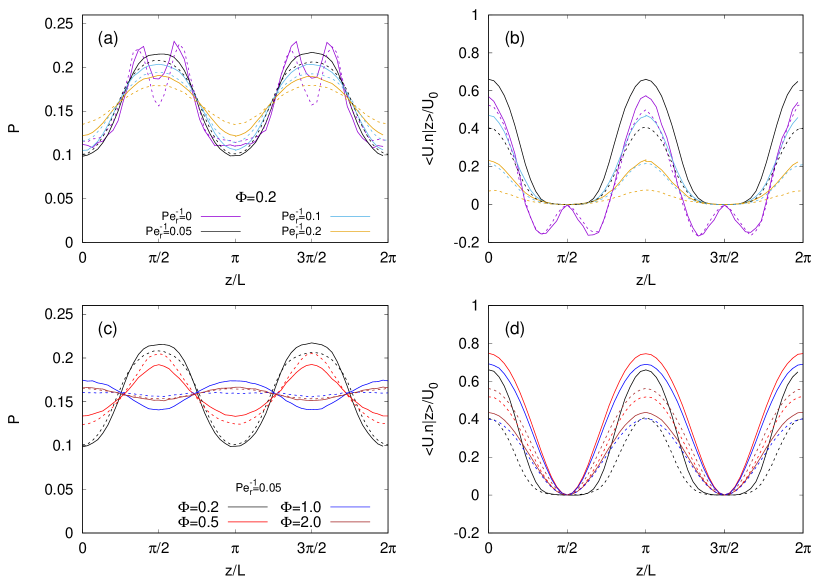
Figure 1: (Color online) Results for the steady Kolmogorov flow. Microswimmer transverse PDF $P(z)$ and alignment in the steady Kolmogorov flow: (a,c) $P(z)$ vs $z/L$, (b,d) $\langle\bm{U}\cdot\bm{n}|z\rangle/U_{0}$ vs $z/L$ for $\Lambda=0.98$. In (a,b) we keep $\Phi=0.2$ fixed and vary the rotational noise, i.e. ${\mathrm{P}e}_{\mathrm{r}}$, as labelled; in (c,d) we keep the rotational noise fixed to ${\mathrm{P}e}_{\mathrm{r}}^{-1}=0.05$ and vary the swimming speed $\Phi$. Solid lines refer to the two-dimensional model, dashed lines to the full three-dimensional one.

We illustrate the phenomenology described above in Fig. 1, where we show (a,c) the probability density function (PDF) of swimmer transverse position, $P(z)$, and (b,d) the conditional average $\langle n_{x}\cos z|z\rangle$ for $\Lambda=0.98$; the reason for choosing $\Lambda<1$ is the presence of a bifurcation point for $\Lambda=1$ at which Eq. (13) possesses marginally stable fixed points, which are of limited physical interest, corresponding to the swimmers oriented along the flow. This behaviour is also reflected in the singularity in Eq. (14). We show the results both for the original deterministic dynamics (12-13) and in the presence of rotational noise that is added to Eq. (13) in the form of a stochastic term, $\sqrt{2{\mathrm{P}e}_{\mathrm{r}}^{-1}}\eta(t)$, where ${\mathrm{P}e}_{\mathrm{r}}=U_{0}/(LD_{\rm r})$ denotes the rotational Péclet number, defined in terms of the rotational diffusion coefficient, $D_{\rm r}$. We remark that the results of simulations of the two-dimensional dynamics (12-13) (solid lines) are qualitatively the same as results of the original dynamics (6-11) in three spatial dimensions (dashed lines).

Figure 1(a) shows that swimmers tend to accumulate in high-shear regions, as also observed in Ref. [7] for Poiseuille flows. As explained in Ref. [7], this phenomenon is physically induced by the fact that the swimmers rotate rapidly, causing them to tumble in small loops in regions of intense shear. Rotational noise can help stabilize this effect [7, 6], as can be seen in Fig. 1(a), where the regions of depletion around $z/L\approx\pi/2$ and $3\pi/2$ disappear in favour of a smooth maximum when a small diffusivity is present. The effect is weakened for larger rotational noise. However, as shown in Fig. 1(c), when the swimming speed is increased, the swimmers instead accumulate in regions with low shear and high flow velocity. The transition between these two regimes is actually quite complex and a detailed study of the dependence on rotational noise, swimming speed and swimmer shape parameter $\Lambda$ is beyond the scope of this work. A complete analysis can be found in Ref. [6], with a detailed study of how the topology of phase space affects the swimmer dynamics in the deterministic case and, for the case with noise, a computation of the joint PDF of $z$ and $\varphi$.

Summarizing the above observations, in a steady Kolmogorov flow we expect swimmers to align with the flow velocity for generic swimming numbers and we expect some form of accumulation (i.e. non-uniform spatial distribution) of the microswimmers. Both effects are robust to the addition of rotational noise to the dynamics. Actually, as shown in Ref. [6], a weak noise has a stabilizing role on the accumulation. This is confirmed by Fig. 1(a), while Fig. 1(b) shows the same effect also on the alignment.

IV Turbulent Kolmogorov flow: numerical simulations

In this Section we study the effect of turbulent fluctuations on accumulation and alignment of microswimmers. Turbulence is a multiscale process, with fluctuations at many length scales, characteristic times and intensity between the large scale defined by the mean flow and the dissipative one, $\eta$ [23]. This is of course very different from the case of a mean flow with rotational diffusion, where there usually is a clear scale separation between the deterministic component of the flow and the short-time-correlated noise associated with the diffusive behaviour. In order to study the effects of turbulent fluctuations on orientation and spatial distribution of swimmers, we performed DNS of the Navier-Stokes equations (1) with Kolmogorov forcing by means of a $2/3$ dealiased, fully parallelized pseudo-spectral code in a cubic, triple-periodic domain for three Reynolds numbers, namely ${\mathrm{R}e}=230,730$ and $1350$. The grid resolution $N$ was chosen as a function of the Kolmogorov scale $\eta$ (see Table 1) to guarantee that $k_{\rm max}\eta\gtrsim 1.23$ for all Reynolds numbers, where $k_{\rm max}=N/3$ is the maximum represented wave-number after de-aliasing. At each time step the values of the velocity field and its gradients were interpolated onto particle positions to integrate the swimmer dynamics (4-5). Both fluid and swimmer equations were advanced with a second-order Runge-Kutta scheme.

$N$	${\mathrm{R}e}$	$U$	$u^{\prime}_{\rm rms}$	$\epsilon$	$\eta$	$\tau_{\eta}$
$128$	$230$	$0.23$	$0.12$	$9.31\times 10^{-4}$	$3.22\times 10^{-2}$	$1.04$
$256$	$730$	$0.73$	$0.38$	$2.30\times 10^{-2}$	$1.44\times 10^{-2}$	$0.21$
$512$	$1350$	$1.35$	$0.76$	$1.73\times 10^{-1}$	$8.72\times 10^{-3}$	$0.076$

Table 1: Parameters used in the DNS of the turbulent Kolmogorov flow. $N$ resolution, $U$ amplitude of the mean profile, ${\mathrm{R}e}=UL/\nu$, $u^{\prime}_{\rm rms}$ rms of the fluctuation of the $x$ component of the velocity, $\epsilon=\nu\langle{\rm Tr}(\mathbb{A}^{\rm T}\mathbb{A})\rangle$ mean energy dissipation, $\eta=(\nu^{3}/\epsilon)^{1/4}$ Kolmogorov scale, $\tau_{\eta}=(\nu/\epsilon)^{1/2}$ Kolmogorov time scale. The integral scale $L=1$ and the viscosity $\nu=10^{-3}$ are fixed for all simulations.

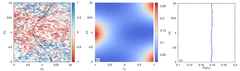
Figure 2: (Color online) Results in the turbulent Kolmogorov flow: (a) swimmers’ orientations in a turbulent simulation at ${\mathrm{R}e}=730$. The swimmers are taken from a slab of thickness $0.4L$ parallel to the mean shear plane. The arrows start from the particle positions and represent the projection of the swimming direction ${\bf n}$ onto the $xz$-plane. The color map codes the intensity of $n_{x}$, i.e. the $x$-component of $n$. The black line displays the mean velocity profile $U\cos(z)$. (b): time averaged joint PDF $P(z,n_{x})$ of swimmer transverse position ($z$) and $n_{x}$ for all the swimmers in the simulation domain. Peaks are due to the alignment of the swimming direction with the mean flow profile. (c) PDF of swimmer transverse positions $P(z)$ obtained from $P(z,n_{x})$ integrated over all possible $n_{x}$. Data refer to swimming number $\Phi=1.09$.

In Fig. 2(a) we plot the instantaneous orientation of the swimmers in a slab of thickness $0.4~{}L$ in the $xz$-plane. The arrows, representing the projection of ${\bf n}$ onto the $xz$-plane, clearly indicate a strong alignment of the instantaneous swimmer orientation with the mean velocity profile, represented by the black solid line, proportional to $\cos z$. In order to better quantify the strength of this alignment, Fig. 2(b) shows the joint PDF $P(z,n_{x})$ of the swimmer position ($z$ coordinate) and swimming direction ($n_{x}$ component). A strong correlation is evident with two peaks at $(z/L,n_{x})=(0,1)$ and $(\pi,-1)$, corresponding to the blue and red arrows in Fig. 2(a), respectively. In spite of the strong correlation between mean velocity and swimming orientation, we do not observe significant preferential accumulation, i.e. swimmers are almost uniformly distributed along the inhomogeneous direction $z$. This is shown in Fig. 2(c), where we plot the distribution of $z$-swimmer positions $P(z)$ obtained by integrating $P(z,n_{x})$ over $n_{x}$. The same phenomenology is observed also for other values of the parameters. This is consistent also with previous results with other orientation mechanisms, such as gyrotaxis, where accumulation in the Kolmogorov flow could be obtained only by artificially reducing the intensity of turbulent fluctuations [10]. We can therefore conclude that preferential alignment is an independent and more robust feature than preferential concentration for microsmimmers in the Kolmogorov flow, since the former is observed in both the laminar and in the turbulent case, while the latter disappears in the turbulent flow. We remark that we do not consider here possible small scale spatial clustering (which is observed for swimming [14] and passivley sedimenting [24] elongated particles in turbulence) but only inhomogeneities in the distribution on the scale of the mean flow.

Figure 3: (Color online) Swimmer alignment in the turbulent Kolmogorov flow. (a) The scalar product $\langle\bm{\beta}\cdot\bm{n}\rangle$ averaged over space and time, as a function of the swimming number $\Phi$ with $\bm{\beta}=\bm{u}$ (purple circles), $\bm{\beta}=\bm{U}$ (green squares) and $\bm{\beta}=\bm{u}^{\prime}$ (blue triangles). The indicated power-law behaviors are obtained from a fit of the points at $\Phi>1$. In the inset, the same quantities are plotted for fixed $\Phi\approx 0.75$ for different ${\mathrm{R}e}$. (b) and (c) Modulation of the correlation between mean fluid velocity (b) or fluctuations (c) and swimmer orientation averaged over $x$, $y$ and time for different swimming numbers. From bottom to top $\Phi=0.54,0.78$ (green curves), $\Phi=1.09$ (red curve), $\Phi=1.27,1.45,1.63,1.92$ (blue curves). Simulation at ${\mathrm{R}e}=730$.

As in the previous section, we evaluate the alignment with the mean flow by computing the scalar product $\langle\bm{U}(\bm{x})\cdot{\bf n}\rangle$ of the swimming vector with the mean fluid velocity, averaged over space and time. However, previous work showed that swimmers can align with the local velocity even in homogeneous turbulence [17]. Such local alignment could in principle disturb the alignment with the mean flow. Following the decomposition of the fluid velocity, Eq. (2), we therefore also consider the alignment with the turbulent fluctuations $\langle\bm{u}^{\prime}(\bm{x},t)\cdot{\bf n}\rangle$ and with the complete fluid velocity $\langle\bm{u}(\bm{x},t)\cdot{\bf n}\rangle$, which is simply the sum of the alignment with the average and fluctuating component (cf. Eq. (2))

$$\langle\bm{u}\cdot\bm{n}\rangle=\langle\bm{U}\cdot\bm{n}\rangle+\langle\bm{u}^{\prime}\cdot\bm{n}\rangle\,.$$ (17)

Figure 3(a) summarizes the statistics of the alignment as a function of the swimming number $\Phi$ for the simulation with ${\mathrm{R}e}=730$. We find that for small values of $\Phi$, the alignment with the mean flow increases linearly with the swimming number. The same behaviour is observed for the alignment with the fluctuations and, as a consequence, with the complete fluid velocity. An alignment proportional to $\Phi$ was already found for an isotropic turbulent flow, in the absence of a mean flow [17]. For larger values of $\Phi$, the alignment with the mean flow increases faster, while that with the full velocity (and fluctuations) is sub-linear. The transition occurs at $\Phi\simeq 1$ (vertical line in Fig. 3). An explanation of the transition is that, for $\Phi>1$, $v_{\mathrm{s}}$ becomes faster than the turbulent velocity, so that flow correlations along swimmer trajectories are dominated by swimming instead of transport by the fluid. As a consequence, the Lagrangian correlation time of fluctuations at scale $\ell$ seen by a swimmer can be estimated as $\ell/v_{\mathrm{s}}$, so the orientation quickly decouples from the small-scale fluctuations, while it remains correlated with the large-scale gradients of the mean flow. In other words, $\langle\bm{U}\cdot\bm{n}\rangle$ increases faster at large $\Phi$ because the chaotic reorientation induced by flow velocity fluctuations becomes less efficient, i.e. they average out.

Panels (b) and (c) in Fig. 3 show the $z$-dependence of alignment through the conditional averages $\langle\bm{U}\cdot\bm{n}|z\rangle$ and $\langle\bm{u}^{\prime}\cdot\bm{n}|z\rangle$ for different values of $\Phi$. In all cases, we observe that $\bm{n}$ is always positively correlated with both the average and fluctuations of the velocity field. Moreover, the correlation increases with $\Phi$, in agreement with the results shown in Fig. 3(a). Since the amplitudes of both the mean flow and fluctuations are modulated along $z$, the profiles observed in Fig. 3(b) and (c) are a combined result of the space dependence of the velocity field and of modulations in the alignment of the swimmers. In the case of the mean flow, Fig. 3(b), the maximal alignment is observed where the flow is large and the gradients are small, i.e. around $z=0$ and $z=\pi$, while in the case of turbulent fluctuations, Fig. 3(c), the alignment is stronger where the mean flow is small, i.e. around $z=\pi/2$ and $z=3\pi/2$.

In order to investigate the dependence of the alignment on the Reynolds number, we show the alignment statistics in the inset of Fig. 3(a) with fixed $\Phi\approx 0.75$ for our three values of ${\mathrm{R}e}$. We observe that the correlation with the mean velocity decreases with ${\mathrm{R}e}$ when rescaled with the typical velocity $u^{\prime}_{\rm rms}$ (which is proportional to $U$ as shown in Table 1), while the correlation with the velocity fluctuations is almost independent on ${\mathrm{R}e}$. This is remarkable since the ratio $U/u^{\prime}_{\rm rms}$ is independent on ${\mathrm{R}e}$ (see Table 1). We comment further on this in the next section.

We remark that in order to have a constant swimming number $\Phi$ for different values of ${\mathrm{R}e}$, the simulations were performed with different swimming speeds, $v_{\mathrm{s}}=\Phi u^{\prime}_{\rm rms}$, which increases with ${\mathrm{R}e}$ (see Table 1). Of course, if interested in describing the effects of turbulence on a specific motile species, we should consider a fixed $v_{\mathrm{s}}$ and we would find that the alignment decreases with ${\mathrm{R}e}$ (not shown). This is in agreement with what has been observed in an isotropic turbulent flow [17] and it is due to the weaker correlation between velocity gradients, which orient the swimming direction, and the velocity field.

V Unsteady Kolmogorov flow: stochastic model

We now move to the statistical model introduced in Sec. II.2, for which we can choose the relative importance of the Eulerian and Lagrangian time scales of the flow by tuning the Kubo number. For small values of $\operatorname{Ku}$, the flow approaches the laminar Kolmogorov flow discussed in Sec. III with a small stochastic noise characterized by the Eulerian time scale $\tau_{\rm f}$. While, in the limit of large $\operatorname{Ku}$, the disturbances become persistent. In this limit the relevant time scale is therefore Lagrangian in nature, because the statistics decorrelates due to transport by the mean flow or through swimming. To compare to our DNS of turbulence, we found, in agreement with previous studies [20, 17], that the Kubo number should be $O(10)$ (larger values give the same results). Further, we match both the Kolmogorov time scale and Taylor length scale in the two flows. Moreover, we choose the parameters $\alpha=1.92$ and $\kappa=0.08$ according to our DNS with ${\mathrm{R}e}=730$ in Table 1. These choices are expected to provide, at least, a qualitative agreement between DNS and the statistical model. A more quantitative agreement could, in principle, be obtained by instead choosing $\alpha$ and $\kappa$ to match relevant properties of flow correlation functions.

\begin{overpic}[width=145.10922pt]{fig_4a.eps} \put(13.0,63.0){(a)} \put(50.0,-6.0){$z/L$} \put(-9.0,31.0){\rotatebox{90.0}{$P(z)$}} \end{overpic}

\begin{overpic}[width=153.6447pt]{fig_4b.eps} \put(13.0,59.0){(b)} \put(50.0,-6.0){$z/L$} \put(-9.0,30.0){\rotatebox{90.0}{$\langle\mbox{\boldmath$U$}\cdot\mbox{\boldmath$n$}|z\rangle/u^{\prime}_{\rm rms}$}} \put(101.0,60.0){\rotatebox{-90.0}{$\langle\mbox{\boldmath$U$}\cdot\mbox{\boldmath$n$}|z\rangle/U$}} \end{overpic}

\begin{overpic}[width=142.26378pt]{fig_4c.eps} \put(13.0,65.0){(c)} \put(50.0,-6.0){$z/L$} \put(-9.0,30.0){\rotatebox{90.0}{$\langle\mbox{\boldmath$u$}^{\prime}\cdot\mbox{\boldmath$n$}|z\rangle/u^{\prime}_{\rm rms}$}} \end{overpic}

Figure 4: (Color online) Microswimmer accumulation and alignment for three-dimensional statistical model simulations for different $\operatorname{Ku}$. (a) distribution of $z$, (b) average $\mbox{\boldmath$U$}\cdot\mbox{\boldmath$n$}$ conditional on $z$, and (c) average $\mbox{\boldmath$u$}^{\prime}\cdot\mbox{\boldmath$n$}$ conditional on $z$. Dashed horizontal lines show the averages (b) $\langle\mbox{\boldmath$U$}\cdot\mbox{\boldmath$n$}\rangle/u^{\prime}_{\rm rms}$ and (c) $\langle\mbox{\boldmath$u$}^{\prime}\cdot\mbox{\boldmath$n$}\rangle/u^{\prime}_{\rm rms}$ without condition on $z$. Parameters: $\Lambda=1$, $\alpha=1.92$, $\kappa=0.08$, and $\Phi=0.54$.

Figure 4 shows spatial accumulation, $P(z)$, and projection on the particle orientation on both the mean flow, $\langle\mbox{\boldmath$U$}\cdot\mbox{\boldmath$n$}|z\rangle$, and the flow fluctuations, $\langle\mbox{\boldmath$u$}^{\prime}\cdot\mbox{\boldmath$n$}|z\rangle$, as functions of $z$. We let $\Phi=0.54$ and use $\alpha$ and $\kappa$ from our DNS. For $\operatorname{Ku}=0.01$, Fig. 4(a) shows that particles accumulate in high-shear regions, just as for the laminar Kolmogorov flow. The degree of accumulation is of the same order as in Fig. 1(a) with small but non-zero inverse Péclet numbers, ${\mathrm{P}e}_{\mathrm{r}}^{-1}$. Small deviations are expected because the noise has different statistics and because the swimming velocity is $v_{\mathrm{s}}/U=0.28$ in Fig. 4(a), while it is $v_{\mathrm{s}}/U=0.2$ in Fig. 1(a). Comparison of Fig. 4(b) (right vertical scale) and Fig. 1(b) shows the same degree of high alignment between the mean flow velocity and the particle orientation, and Fig. 4(c) shows that the alignment with the stochastic part of the flow is negligible for small values of $\operatorname{Ku}$.

For larger values of $\operatorname{Ku}$, $\operatorname{Ku}=10$, we compare to our DNS results. Similar to the DNS in Fig. 2(c), the stochastic fluctuations at large $\operatorname{Ku}$ ruin the accumulation observed for small values of $\operatorname{Ku}$ and particles are essentially uniformly distributed. Moreover, we find that $\langle\mbox{\boldmath$U$}\cdot\mbox{\boldmath$n$}|z\rangle$ and $\langle\mbox{\boldmath$u$}^{\prime}\cdot\mbox{\boldmath$n$}|z\rangle$ in Fig. 4(b,c) are both in qualitative agreement with the DNS data with $\Phi=0.54$ in Fig. 3(b,c), though the details do not match. The alignment $\langle\mbox{\boldmath$U$}\cdot\mbox{\boldmath$n$}|z\rangle$ is approximately a factor 2 times larger in the statistical model, and $\langle\mbox{\boldmath$u$}^{\prime}\cdot\mbox{\boldmath$n$}|z\rangle$ is somewhat smaller and stronger modulated than the DNS results.

In conclusion, our results for the statistical model qualitatively interpolates between the laminar Kolmogorov flow results for small values of $\operatorname{Ku}$ and the DNS results for large values of $\operatorname{Ku}$. For intermediate values of $\operatorname{Ku}$, the alignment $\langle\mbox{\boldmath$U$}\cdot\mbox{\boldmath$n$}|z\rangle$ has a minimum somewhere around $\operatorname{Ku}\sim 1$, while $\langle\mbox{\boldmath$u$}^{\prime}\cdot\mbox{\boldmath$n$}|z\rangle$ increases monotonously with $\operatorname{Ku}$.

The results in Fig. 4(b,c) show that the alignment conditional on $z$ is essentially obtained by a periodic modulation of the unconditional alignment. As observed in the DNS simulations, alignment with the fluctuations is maximal around the zeroes of the mean flow, where the mean gradients are lager. To investigate how the unconditional alignment changes with the parameters of the dynamics, we decompose the projection of the flow velocity on the direction of the swimmer into the contributions from the mean and the fluctuations (17). As already discussed, swimming breaks the fore-aft symmetry, allowing the average alignment to take non-zero values. For the case without the mean flow, $U=0$, the perturbation theory of Ref. [17] gives an estimate of $\langle\mbox{\boldmath$u$}^{\prime}\cdot\mbox{\boldmath$n$}\rangle$ and explains the alignment between $\mbox{\boldmath$u$}^{\prime}$ and $n$. When a mean flow is present, perturbation theory is much harder. As we remarked in Section III, the limit $\Phi\to 0$ is singular in the deterministic dynamics. Moreover, Fig. 1 shows that as ${\mathrm{P}e}_{\mathrm{r}}^{-1}$ approaches zero, the alignment abruptly changes behavior, making the limit $\operatorname{Ku}\to 0$ singular as well. Therefore, instead of making a perturbation theory around the deterministic solutions found in Section III, we consider a perturbation theory in terms of small $\alpha=U/u^{\prime}_{\rm rms}$ and $\Phi=v_{\mathrm{s}}/u^{\prime}_{\rm rms}$ around the limit of tracer particles advected by the stochastic part of the fluid velocity. In this limit, we expect the second term in Eq. (17), $\langle\mbox{\boldmath$u$}^{\prime}\cdot\mbox{\boldmath$n$}\rangle$, to be mainly unaffected compared to the $\alpha=0$ case studied in Ref. [17]. We argue that for small $\kappa$, $\alpha$ and $\Phi$, the first term of Eq. (17) takes the form

$$\frac{\langle\mbox{\boldmath$U$}\cdot\mbox{\boldmath$n$}\rangle}{u^{\prime}_{\rm rms}}\sim{\mathcal{C}}_{\Lambda}\kappa^{2}\alpha^{2}\Phi\,,$$ (18)

where the coefficient ${\mathcal{C}}_{\Lambda}$ depends on the flow and the particle shape. The rationale for the above expression is as follows.

First, using the symmetry of the dynamics (4) and (5) under the joint transformation $v_{\mathrm{s}}\to-v_{\mathrm{s}}$ and $\mbox{\boldmath$n$}\to-\mbox{\boldmath$n$}$, $\langle\mbox{\boldmath$u$}^{\prime}\cdot\mbox{\boldmath$n$}\rangle$ must be an odd function of $\Phi$, scaling linearly with $\Phi$ for small values of $\Phi$ [17]. The same argument applies to $\langle\mbox{\boldmath$U$}\cdot\mbox{\boldmath$n$}\rangle$, giving the linear scaling in Eq. (18). For the Kolmogorov mean flow, $U_{x}=U\cos(z/L)$, the average projection on $n$ is invariant under reversing the sign of either the velocity field, $U\to-U$, or the box length, $L\to-L$. Hence, $\langle\mbox{\boldmath$U$}\cdot\mbox{\boldmath$n$}\rangle$ must be an even function in both $U$ and $L$, implying it is also even in $\alpha$ and $\kappa$. When $\alpha=0$, there is no mean flow to align with and the lowest contributing order in Eq. (18) is thus quadratic. When $\kappa=0$, the mean flow is constant and, since a constant mean flow is not physically distinguishable from a flow without a mean, the alignment must vanish for this case, meaning that Eq. (18) is quadratic to lowest order in $\kappa$ in a physical flow. As noted in Sec. II.2, $\kappa\propto{\rm Re}^{-1/2}$, so Eq. (18) implies that alignment with the mean flow decreases with ${\rm Re}$, as indeed observed in our DNS (see inset of Fig. 3(a)). However, the alignment decreases somewhat slower than predicted by the $\kappa^{2}$ scaling, indicating that the coefficient $C_{\Lambda}$ increases with ${\mathrm{R}e}$. It is expected that $C_{\Lambda}$ depends on the statistics of the stochastic part of the flow, and hence on ${\mathrm{R}e}$ for the turbulence simulations and on $\operatorname{Ku}$ in the statistical model. Finally, the coefficient $C_{\Lambda}$ also depends on the shape factor $\Lambda$. When $\Lambda=0$, the swimmer becomes spherical and does not couple to the strain part of the mean flow. We therefore expect that the coefficient ${\mathcal{C}}_{\Lambda}$ goes to zero as $\Lambda\to 0$.

\begin{overpic}[width=165.02606pt]{fig_5a.eps} \put(14.0,65.0){(a)} \put(50.0,30.0){$\sim\alpha^{2}$} \put(50.0,-6.0){$\alpha$} \put(-8.0,32.0){\rotatebox{90.0}{$\langle\mbox{\boldmath$\beta$}\cdot\mbox{\boldmath$n$}\rangle/u^{\prime}_{\rm rms}$}} \end{overpic}

\begin{overpic}[width=165.02606pt]{fig_5b.eps} \put(14.0,65.0){(b)} \put(50.0,-6.0){$\Phi$} \put(40.0,35.0){$\sim\Phi$} \end{overpic}

\begin{overpic}[width=169.29381pt]{fig_5c.eps} \put(88.0,64.0){(c)} \put(50.0,-6.0){$\operatorname{Ku}$} \end{overpic}

Figure 5: (Color online) Statistical model simulations of average projection $\langle\mbox{\boldmath$\beta$}\cdot\mbox{\boldmath$n$}\rangle$, with $\mbox{\boldmath$\beta$}=\mbox{\boldmath$U$}$ (green,$\Box$) and $\mbox{\boldmath$\beta$}=\mbox{\boldmath$u$}^{\prime}$ (blue,$\vartriangle$). The data is plotted against the dimensionless scale of (a) the mean flow velocity $\alpha$, (b) swimming speed $\Phi$ and (c) the Kubo number $\operatorname{Ku}$. The solid green lines show Eq. (18) with a coefficient ${\cal C}_{\Lambda}=23$ fitted for small $\alpha$, $\Phi$ and $\kappa$ in panel (a). Dashed blue lines show simulation results of $\langle u^{\prime}\cdot\mbox{\boldmath$n$}\rangle$ for the case of no mean flow, $\alpha=0$. The dotted green line in panel (c) shows results of $\langle\mbox{\boldmath$U$}\cdot\mbox{\boldmath$n$}\rangle$ in the deterministic limit [Eqs. (6–11)] (converted to the dimensional units used here). Parameters: $\Lambda=1$, $\kappa=0.08$, (a,b) $\operatorname{Ku}=10$, (a,c) $\Phi=0.3$, and (b,c) $\alpha=1.92$.

Unlike DNS of the Kolmogorov flow, the statistical model allows to freely choose the dimensionless parameters $\alpha$ and $\kappa$. To verify the form (18), we therefore use statistical model simulations of rod-like swimmers, $\Lambda=1$, in three spatial dimensions. Fig. 5(a) shows results of $\langle\mbox{\boldmath$U$}\cdot\mbox{\boldmath$n$}\rangle$ and $\langle\mbox{\boldmath$u$}^{\prime}\cdot\mbox{\boldmath$n$}\rangle$ against $\alpha$ with small $\Phi$ and $\kappa$. The solid green line shows Eq. (18) with a fitted prefactor ${\cal C}_{\Lambda}=23$ for our parameters $\operatorname{Ku}=10$ and $\Lambda=1$. We observe that the predicted quadratic scaling of $\langle\mbox{\boldmath$U$}\cdot\mbox{\boldmath$n$}\rangle$ with small $\alpha$ qualitatively agrees with the simulation data all the way up to the value $\alpha=1.92$ of the DNS. The alignment with the stochastic part, $\langle\mbox{\boldmath$u$}^{\prime}\cdot\mbox{\boldmath$n$}\rangle$, is only weakly affected by the mean flow. For $\alpha<2$, it is approximately equal to the value obtained without mean flow (dashed blue line).

In Fig. 5(b) we show the same quantities against $\Phi$ for the value $\alpha=1.92$ of our DNS with ${\mathrm{R}e}=730$. Even though $\alpha$ is not small, the symmetry argument after Eq. (18) anyway implies a linear scaling of $\langle\mbox{\boldmath$U$}\cdot\mbox{\boldmath$n$}\rangle$ with $\Phi$ for small values of $\Phi$, but the prefactor is somewhat smaller compared to Eq. (18) with ${\cal C}_{\Lambda}=23$ (solid green line) The alignment $\langle\mbox{\boldmath$u$}^{\prime}\cdot\mbox{\boldmath$n$}\rangle$ is approximately the same as for the case $\alpha=0$ (dashed blue line), showing a linear scaling for small $\Phi$ as predicted in Ref. [17]. Similar to for Fig. 4, our results agree qualitatively with the results in the DNS if $\Phi<1$, but $\langle\mbox{\boldmath$U$}\cdot\mbox{\boldmath$n$}\rangle$ comes out larger and $\langle\mbox{\boldmath$u$}^{\prime}\cdot\mbox{\boldmath$n$}\rangle$ comes out smaller than the DNS in Fig. 3. For $\Phi$ larger than $\sim 1$, the alignment decreases in the statistical model, while it increases in the DNS. The reason for this difference is the presence of the inertial range in a turbulent flow, with fluctuations over different scales and times. Such range is not present in the statistical model where the fluctuations take place on a single length scale.

Figure 5(c) shows how the alignment changes from the limit of laminar Kolmogorov flow at small $\operatorname{Ku}$ to the limit of a turbulent Kolmogorov flow at large $\operatorname{Ku}$. Since $\tau_{\rm f}$ is not a relevant time scale in the latter limit, plateaus are formed in both alignments $\langle\mbox{\boldmath$U$}\cdot\mbox{\boldmath$n$}\rangle$ and $\langle\mbox{\boldmath$u$}^{\prime}\cdot\mbox{\boldmath$n$}\rangle$ for large $\operatorname{Ku}$. When $\operatorname{Ku}=0$, the flow is deterministic and the dynamics discussed in Section III applies. The green dotted line in Fig. 5(c) shows simulation results of $\langle\mbox{\boldmath$U$}\cdot\mbox{\boldmath$n$}\rangle$ in the deterministic limit [Eqs. (6–11)], scaled to the units used in this section. The numerical data indicates that the deterministic limit is singular: the average with $\operatorname{Ku}=0$ is not approached smoothly for small but finite values of $\operatorname{Ku}$. This is consistent with the behavior in Fig. 1 (b), where a small noise abruptly changes the spatial dependence of the alignment. As observed in Fig. 4(b), $\langle\mbox{\boldmath$U$}\cdot\mbox{\boldmath$n$}\rangle$ is non-monotonic, having a large alignment for both small and large values of $\operatorname{Ku}$ with a minimum around $\operatorname{Ku}\sim 1$. The mechanism is however different in the two limits, for small $\operatorname{Ku}$ the alignment is purely determined by the mean flow $U$, while in the limit of large $\operatorname{Ku}$ the contributions from the mean flow and the stochastic part are of the same order. The alignment $\langle\mbox{\boldmath$u$}^{\prime}\cdot\mbox{\boldmath$n$}\rangle$ is approximately given by the case without mean flow (dashed blue line).

In summary, the numerical data of the statistical model show a linear scaling with $\Phi$ and a quadratic scaling with $\alpha$, as predicted by Eq. (18). The $\kappa^{2}$ scaling is hard to verify with $\alpha=1.92$ using the statistical model. We instead verify this scaling for the case of smaller values of $\alpha$ below.

V.1 Perturbation theory in two spatial dimensions

To understand the physical mechanisms that give rise to the alignment, we evaluate ${\mathcal{C}}_{\Lambda}$ analytically in the statistical model for small values of $\operatorname{Ku}$ in two spatial dimensions. To this end we make a series expansion around the limit where the dynamics is dominated by the stochastic part of the velocity field (i.e. small $\alpha$). In addition we consider both $\kappa$ and $\Phi$ small consistently with the limit in Eq. (18), and we assume that the Kubo number is small in order to close the expansion at second order in $\operatorname{Ku}$. The computation is done with the further assumption that both $\alpha$ and $\Phi$ are small enough compared to $\operatorname{Ku}$, so that the periodic trajectories in the deterministic dynamics can be neglected. The perturbation theory follows the method introduced in Refs. [25, 26, 27, 28] and reviewed in [20], but with one important difference: we expand the angular dynamics around the solution $\varphi^{(0)}(t)$ obtained if the mean flow gradients are set to zero and if the stochastic part of the flow gradients are evaluated at a fixed position. Even though $\varphi^{(0)}(t)$ is a function of $\operatorname{Ku}$, we do not expand trigonometric functions of $\varphi^{(0)}(t)$ in terms of small $\operatorname{Ku}$. As a result, we avoid secular terms and the resulting solution converges for large times. The details of the expansion are given in Appendix A. The general result from our expansion is obtained in Eq. (34) and reported below

$$\frac{\langle\mbox{\boldmath$U$}\cdot\mbox{\boldmath$n$}\rangle}{u^{\prime}_{\rm rms}} =\frac{1}{2}\Phi\Lambda\int\frac{{\rm d}^{2}\mbox{\boldmath$y$}}{(2\pi L)^{2}}{\rm Tr}(\mathbb{S}(\mbox{\boldmath$y$})^{2})\int_{0}^{t}{\rm d}t_{1}\int_{0}^{t_{1}}{\rm d}t_{2}$$ (19)

$$\times\exp\left[-\frac{2+\Lambda^{2}}{8}\left[\int_{t_{2}}^{t}{\rm d}t^{\prime}\int_{t_{2}}^{t}{\rm d}t^{\prime\prime}C(t^{\prime}-t^{\prime\prime})+\int_{t_{2}}^{t_{1}}{\rm d}t^{\prime}\int_{t_{2}}^{t_{1}}{\rm d}t^{\prime\prime}C(t^{\prime}-t^{\prime\prime})+2\int_{t_{2}}^{t}{\rm d}t^{\prime}\int_{t_{2}}^{t_{1}}{\rm d}t^{\prime\prime}C(t^{\prime}-t^{\prime\prime})\right]\right]\,.$$

This expression applies to a general mean flow that is either periodic or zero at the boundaries of a box of side length $2\pi L$. It consists of one spatial average over the squared mean-flow strain, ${\rm Tr}(\mathbb{S}(\mbox{\boldmath$y$})^{2})$, where $\mathbb{S}$ has components $S_{ij}=(\partial_{j}U_{i}+\partial_{i}U_{j})/2$, multiplied by time integrals of the correlation function of the stochastic fluid gradients evaluated at a fixed position $\mbox{\boldmath$x$}_{0}$, $C(t)=\langle\partial_{j}u^{\prime}_{i}(\mbox{\boldmath$x$}_{0},t)\partial_{j}u^{\prime}_{i}(\mbox{\boldmath$x$}_{0},0)\rangle$. In the derivation of Eq. (19), the mean part of the flow has been evaluated at fixed positions (instead of Lagrangian trajectories), which is a valid approximation for small values of $\operatorname{Ku}$, but may fail when $\operatorname{Ku}$ is large.

Equation (19) converges in the limit of large time. In contrast, perturbation theory of angular dynamics in terms of small $\operatorname{Ku}$ in previous studies gave rise to secular terms [26, 27, 28]. In these cases a self-consistency condition was used to remove the secular terms, leading to infinite recursion relations that can only be solved in limiting cases. We expect that the solution method introduced here will apply to a large number of problems that were not accessible using the old method, including solving the angular dynamics in Refs. [26, 27, 28] without reference to infinite recursion relations.

Using the correlation function of the stochastic model allows to evaluate Eq. (19) to lowest contributing order in $\operatorname{Ku}$ (see Appendix A for details)

$$\frac{\langle\mbox{\boldmath$U$}\cdot\mbox{\boldmath$n$}\rangle}{u^{\prime}_{\rm rms}}=\frac{\Lambda}{2(2+\Lambda^{2})^{2}\operatorname{Ku}^{2}}\kappa^{2}\alpha^{2}\Phi\,.$$ (20)

This expression is on the form (18) with ${\mathcal{C}}_{\Lambda}=\Lambda/(2(2+\Lambda^{2})^{2}\operatorname{Ku}^{2})$. We remark that since $\alpha$ and $\Phi$ are assumed to be small enough compared to $\operatorname{Ku}$, the inverse dependence on $\operatorname{Ku}^{2}$ in Eq. (20) does not pose a problem to the expansion.

It is instructive to analyze what mechanisms contribute to Eq. (19). First, we find that the flow velocity in the translational dynamics (4) does not contribute, and to order $\operatorname{Ku}^{2}$ the translational dynamics is implicitly determined by the orientation through $\mbox{\boldmath$x$}(t)=\mbox{\boldmath$x$}_{0}+\int_{0}^{t}{\rm d}t_{1}v_{\mathrm{s}}\mbox{\boldmath$n$}(t_{1})$. As a consequence, displacement due to the mean flow does not contribute to Eq. (19). The displacement due to swimming affects the sampling of the factor $U$ in $\langle\mbox{\boldmath$U$}\cdot\mbox{\boldmath$n$}\rangle$, but also the factor $n$ due to a feed-back from swimming on the sampling of mean-flow gradients in the rotational dynamics (5). If the displacement due to swimming were not taken into account, the rotational dynamics would essentially originate from Jeffery’s orbits driven by time-dependent fluid gradients. But in that case $\langle\mbox{\boldmath$U$}\cdot\mbox{\boldmath$n$}\rangle$ must vanish. The feedback due to displacement from swimming shows that the alignment with the mean flow is a more intricate effect.

Second, the vorticity of the mean flow does not contribute to Eq. (19). The alignment is instead determined by the mean-flow strain, and there is a net alignment in any flow where the spatial average in Eq. (19) is non-zero. On the other hand, in the contribution from the stochastic part of the flow to Eq. (19), vorticity is the dominant contribution for all values of $\Lambda$, and the sole contribution for small values of $\Lambda$. This is simply a consequence of the strain being multiplied by the shape factor $\Lambda$ in Jeffery’s orientational dynamics (5) and by a cancellation between strain components multiplying different trigonometric functions of the angle. We conclude by observing that in Fig. 4(b), swimmers show the largest alignment where the mean flow is high and the flow gradients are small. It may therefore be perceived as surprising that it is the mean strain gradients rather than the mean flow that determines the mean alignment.

Third, we find that preferential sampling of the stochastic part of the flow does not contribute to Eq. (19), implying that the stochastic flow and its gradients can be evaluated at a fixed position. This is in contrast to the alignment with the stochastic part of the flow. We have made an expansion similar to that leading to Eq. (19), but for the stochastic part, $\langle\mbox{\boldmath$u$}^{\prime}\cdot\mbox{\boldmath$n$}\rangle$. This expansion shows that $\langle\mbox{\boldmath$u$}^{\prime}\cdot\mbox{\boldmath$n$}\rangle$ is not affected by the mean flow to lowest contributing order in $\operatorname{Ku}$. Without a mean flow, the alignment was derived for small $\operatorname{Ku}$ in Ref. [17]:

$$\frac{\langle\mbox{\boldmath$u$}^{\prime}\cdot\mbox{\boldmath$n$}\rangle}{u^{\prime}_{\rm rms}}=\Phi\Lambda\operatorname{Ku}^{2}\,.$$ (21)

As discussed in Ref. [17], this alignment requires preferential sampling of the stochastic fluctuations of the flow.

Although Eq. (19) is derived for small values of $\operatorname{Ku}$, we use the scaling $\langle\mbox{\boldmath$U$}\cdot\mbox{\boldmath$n$}\rangle\sim\alpha(\kappa\alpha)(\kappa\Phi)$ in Eq. (18) to argue that the same mechanisms are, at least for small $\alpha$ and $\Phi$, dominant in general flows dominated by fluctuations, such as our DNS. The first factor $\alpha$ trivially comes from $U$ in $\langle\mbox{\boldmath$U$}\cdot\mbox{\boldmath$n$}\rangle/u_{\rm rms}$. There are two ways $\kappa$ can enter the dynamics: either from derivatives of the mean flow, which are proportional to $\kappa\alpha$, or from the feedback from the swimming on the location of the swimmer in the mean flow, which gives a factor $\kappa\Phi$. We therefore expect the flow in the translational dynamics to be negligible compared to the swimming, and the swimming to have a feedback on the rotational dynamics, just as for small $\operatorname{Ku}$ above.

\begin{overpic}[width=130.08731pt]{fig_6a.eps} \put(14.0,64.0){(a)} \put(50.0,-6.0){$\Phi$} \put(-8.0,30.0){\rotatebox{90.0}{$\langle\mbox{\boldmath$U$}\cdot\mbox{\boldmath$n$}\rangle/u^{\prime}_{\rm rms}$}} \end{overpic}

\begin{overpic}[width=130.08731pt]{fig_6b.eps} \put(14.0,64.0){(b)} \put(50.0,-6.0){$\alpha$} \put(-8.0,30.0){\rotatebox{90.0}{$\langle\mbox{\boldmath$U$}\cdot\mbox{\boldmath$n$}\rangle/u^{\prime}_{\rm rms}$}} \end{overpic}

\begin{overpic}[width=130.08731pt]{fig_6c.eps} \put(14.0,64.0){(c)} \put(50.0,-6.0){$\kappa$} \put(-8.0,30.0){\rotatebox{90.0}{$\langle\mbox{\boldmath$U$}\cdot\mbox{\boldmath$n$}\rangle/u^{\prime}_{\rm rms}$}} \end{overpic}

\begin{overpic}[width=130.08731pt]{fig_6d.eps} \put(14.0,64.0){(d)} \put(50.0,-6.0){$\Lambda$} \put(-8.0,30.0){\rotatebox{90.0}{$\langle\mbox{\boldmath$U$}\cdot\mbox{\boldmath$n$}\rangle/u^{\prime}_{\rm rms}$}} \end{overpic}

\begin{overpic}[width=133.1243pt]{fig_6e.eps} \put(14.0,62.0){(e)} \put(50.0,-6.0){$\operatorname{Ku}$} \put(-8.0,30.0){\rotatebox{90.0}{$\langle\mbox{\boldmath$\beta$}\cdot\mbox{\boldmath$n$}\rangle/u^{\prime}_{\rm rms}$}} \end{overpic}

Figure 6: (Color online) Test of analytical predictions. (a–d) Average projection of $U$ onto the direction $n$ plotted against (a) the swimming speed $\Phi$, (b) mean flow magnitude $\alpha$, (c) wave number $\kappa$, and (d) shape factor $\Lambda$ for small $\operatorname{Ku}$. Numerical data from the stochastic model in two spatial dimensions are plotted as markers. Solid lines show the theory (20) and dotted lines in panel (a) show the large-$\Phi$ theory (22). Panel (e) shows data corresponding to Fig. 5(c), but in two spatial dimensions with small $\alpha$ and $\Phi$. The solid lines show the theory (20) [green] and (21) [blue]. Panel (a): $\alpha=0.071$ (red,$\circ$), $\alpha=0.14$ (green,$\Box$), $\alpha=0.28$ (blue,$\Diamond$), and $\alpha=0.71$ (magenta,$\vartriangle$). Panel (b): $\Phi=0.071$ (red,$\circ$), $\Phi=0.14$ (green,$\Box$), $\Phi=0.28$ (blue,$\Diamond$), and $\Phi=0.71$ (magenta,$\vartriangle$). Panels (c,d): $\alpha=\Phi=0.071$ (red,$\circ$), $\alpha=\Phi=0.14$ (green,$\Box$), $\alpha=\Phi=0.28$ (blue,$\Diamond$), and $\alpha=\Phi=0.71$ (magenta,$\vartriangle$). Panel (e): $\alpha=\Phi=0.14$. Panels (a–c,e): $\Lambda=0.98$. Panels (a–b,d–e): $\kappa=0.22$. Panels (a–d): $\operatorname{Ku}=0.1$.

V.2 Comparison of analytical theory with numerical simulations

Equation (20) is compared to numerical simulations with small values of $\operatorname{Ku}$ in Fig. 6. We observe good agreement in general, but there is a systematic trend of the theory to overpredict the alignment. A plausible explanation for this is that these deviations come from a higher-order additive contribution.

Figures 6(a–c) show that the predicted scaling $\langle\mbox{\boldmath$U$}\cdot\mbox{\boldmath$n$}\rangle/u^{\prime}_{\rm rms}\sim\kappa^{2}\alpha^{2}\Phi$ agrees well with the theory (20) for small enough $\Phi$, $\alpha$, and $\kappa$. For large $\Phi$, panel (a) also shows the theory

$$\frac{\langle\mbox{\boldmath$U$}\cdot\mbox{\boldmath$n$}\rangle}{u^{\prime}_{\rm rms}}=\frac{\Lambda\alpha^{2}}{2\Phi}$$ (22)

for large swimming speeds (dashed lines), which is derived in Appendix B. This expression is valid if $\Phi$ is large compared to $\alpha$ and unity. Moreover, it does not depend on the Kubo number and thus it applies also to Fig. 5(b), up to a change in the prefactor due to the spatial dimension (not shown). The theory (22) works well for the statistical model, but it is expected to fail in the DNS due to long-range spatial correlations in the inertial range, not present in the statistical model, c.f. Fig 3. Figure 6(d) shows the shape dependence of the alignment for small $\operatorname{Ku}$. The theory agrees well if $\alpha$ and $\Phi$ are small. Equation (20) shows that $\langle\mbox{\boldmath$U$}\cdot\mbox{\boldmath$n$}\rangle$ is linear in $\Lambda$ for small values of $\Lambda$, and approximately independent of $\Lambda$ for $\Lambda\gtrsim 0.5$ where it reaches $90\%$ of its maximal value. This further motivates our choice of $\Lambda=1$ in the DNS simulations, at least for small values of $\operatorname{Ku}$. Finally, Fig. 6(e) shows how the alignment depends on $\operatorname{Ku}$. The theory agrees for small values of $\operatorname{Ku}$, but fails for the deterministic part when $\operatorname{Ku}$ becomes very small, $\operatorname{Ku}\sim 0.01$. The reason is that periodic orbits are formed when $\operatorname{Ku}$ is not large enough compared to $\Phi$ and $\alpha$, which are not included in the theory. For very large values of $\operatorname{Ku}$, the system obtains very large alignment. This is a result of periodic orbits of elongated swimmers in frozen two-dimensional stochastic flows. This effect is not present in the 3D simulations in Fig. 5(c) because the dynamics of elongated swimmers in 3D frozen flows is chaotic. Equations (20) and (21) are equal at the scale $\operatorname{Ku}_{\rm c}=2^{-1/4}\sqrt{\kappa\alpha/(2+\Lambda^{2})}$ for small values of $\kappa$, $\alpha$ and $\operatorname{Ku}$. Below this scale, alignment is dominated by the mean part of the flow and, above it, the alignment with the stochastic part of the flow dominates. This scale also explains the locations of the cross-over in the 3D simulations with larger $\alpha$, $\operatorname{Ku}_{\rm c}\approx 0.2$, consistent with the results in Fig. 5(c). We conclude by remarking that the alignment with the stochastic part of the velocity in Fig. 6(e) is indistinguishable to the case with $\alpha=0$ (dashed blue line), consistent with our theory for the stochastic part that is independent of $\alpha$ to lowest order in $\operatorname{Ku}$.

VI Conclusions

We investigated the statistics of accumulation and alignment of elongated microswimmers in an inhomogeneous Kolmogorov flow. We used different techniques to address three specific situations. In the case of a laminar, steady flow, we used a dynamical systems approach together with numerical simulations to study the effect of a small rotational diffusivity. In this case, we observe a robust alignment of the swimming direction with the underlying flow together with a non-homogeneous distribution of swimmers which tend to accumulate in regions of high shear.

The case of turbulent Kolmogorov flow is studied by means of DNS of the Navier-Stokes equations. In this case, we find that swimmers are still able to align with the direction of the mean flow in spite of the presence of turbulent fluctuations. Interestingly, we observe an alignment also with the local turbulent velocity fluctuations, which confirm the results recently obtained for an homogeneous isotropic flow [17]. On the contrary, the accumulation of swimmers in high shear regions is disrupted by the presence of turbulent fluctuations for all the values of the parameters investigated.

In order to interpolate between these two regimes, we also considered a steady Kolmogorov flow with an overlying stochastic component. In this case we are able to develop an analytic perturbative approach which describes the origin of the observed alignment in a variety of limits. Remarkably, the alignment with the mean flow finds its roots in the mean strain and the fluctuating vorticity. In contrast the alignment with the stochastic part of the flow is not affected by the mean flow but it is determined by the fluctuating strain.

Our results indicate that elongated microswimmers are able to align their swimming direction with the mean flow in a wide range of conditions and we expect that a similar behavior should be observable in other shear flows. For example Eq. (18), together with the definitions of $\kappa$ and $\alpha$, suggests that the alignment-induced contribution of the mean flow to the displacement of swimmers can be estimated by $\langle\bm{U}\cdot\bm{n}\rangle\approx C\tau_{\eta}^{2}S^{2}v_{\mathrm{s}}$, with $S$ the local shear rate and $C$ a Reynolds-dependent parameter that is O(10) for our flow (see section V). In the presence of strong stratification, vertical structures of velocity profiles are observed in the ocean at a scale of about $5$–$10\,{\rm m}$, with shear rates of order $S=0.01\,{\rm s}^{-1}$, corresponding to typical velocities in the range $5$–$10\,{\rm cm/s}$ [29, 30]. In the ocean, in weakly turbulent conditions, one can have $\epsilon\sim 10^{-9}\,\mathrm{J}\,\mathrm{kg}^{-1}\,\mathrm{s}^{-1}$ [31, 32], giving $\tau_{\eta}^{2}\sim 10^{3}\mathrm{s}^{2}$. For such values of $\epsilon$ typical $u^{\prime}_{\rm rms}$ range between $0.3$–$1\,{\rm cm/s}$ [33]. Based on these estimates one gets $\langle\bm{U}\cdot\bm{n}\rangle\sim O(v_{\mathrm{s}})$. Single-celled motile organisms can swim at speeds up to $v_{\mathrm{s}}=200$–$300\mu{\rm m/s}$. Some phytoplankters can form elongated chains of up to 10 cells which can reach $v_{\mathrm{s}}=1.5\,{\rm mm/s}$ [34]. Thus, the alignment with the mean flow can impact the dispersion properties of microswimmers in weak turbulence also in the absence of accumulation, widening the previous observations made in steady flows [13].

Appendix A Perturbation expansion in small Kubo numbers

To make a perturbation expansion in terms of small values of $\operatorname{Ku}$, we dedimensionalize the dynamics (1-5) in terms of the flow scales in the stochastic model in Section II.2, i.e. time is dedimensionalized by $\tau_{\rm f}$, space by $\ell_{\rm f}$ and velocity by $u_{\rm f}$. In these units the dynamics in two spatial dimensions becomes

$$\begin{split}\dot{\mbox{\boldmath$x$}}_{t}&=\operatorname{Ku}[\mbox{\boldmath$u$}(\mbox{\boldmath$x$}_{t},t)+\Phi\mbox{\boldmath$n$}_{t}]\,,\\ \dot{\varphi}_{t}&=\operatorname{Ku}[\mbox{\boldmath$n$}^{\perp}_{t}]^{\rm T}\mathbb{B}(\mbox{\boldmath$x$}_{t},t)\mbox{\boldmath$n$}_{t}\,,\end{split}$$ (23)

where $\mbox{\boldmath$n$}^{\perp}=(-\sin\varphi,\cos\varphi)$ is a unit vector perpendicular to $n$ and $\mathbb{B}=\mathbb{O}+\Lambda\mathbb{S}$, with $\mathbb{O}=(\mathbb{A}-\mathbb{A}^{\rm T})/2$ and $\mathbb{S}=(\mathbb{A}+\mathbb{A}^{\rm T})/2$ being the antisymmetric and symmetric part of the fluid gradient matrix $\mathbb{A}$. We use subscripts of $t$ to denote functional dependence on time, for example $\mbox{\boldmath$x$}_{t}=\mbox{\boldmath$x$}(t)$. In this appendix we denote the mean and stochastic part of the flow and its gradients evaluated at the initial position $\mbox{\boldmath$x$}_{0}$ by

$$\mbox{\boldmath$u$}(\mbox{\boldmath$x$}_{0},t)=\mbox{\boldmath$U$}(\mbox{\boldmath$x$}_{0})+\mbox{\boldmath$u$}(t)\hskip 14.22636pt\mbox{and}\hskip 14.22636pt\mathbb{A}(\mbox{\boldmath$x$}_{0},t)=\mathbb{A}(\mbox{\boldmath$x$}_{0})+\mathbb{A}(t)\,,$$ (24)

i.e. a spatial argument denotes the mean part of the flow and a time argument the stochastic part of the flow at position $\mbox{\boldmath$x$}_{0}$. By decomposing $\mathbb{B}(\mbox{\boldmath$x$}_{t},t)$ in terms of its stochastic part at the initial position $\mbox{\boldmath$x$}_{0}$, $\mathbb{B}(t)$, and the remainder $\mathbb{B}(\mbox{\boldmath$x$}_{t},t)-\mathbb{B}(t)$, we write the implicit solution to Eq. (23) as

$$\begin{split}\mbox{\boldmath$x$}_{t}&=\mbox{\boldmath$x$}_{0}+\operatorname{Ku}\int_{0}^{t}{\rm d}t_{1}\left[\mbox{\boldmath$u$}(\mbox{\boldmath$x$}_{t_{1}},t_{1})+\Phi\mbox{\boldmath$n$}_{t_{1}}\right]\,,\\ \varphi_{t}&=\varphi^{(0)}_{t}+\operatorname{Ku}\int_{0}^{t}{\rm d}t_{1}\left[-[\mbox{\boldmath$n$}^{\perp,(0)}_{t_{1}}]^{\rm T}\mathbb{B}(t_{1})\mbox{\boldmath$n$}^{(0)}_{t_{1}}+[\mbox{\boldmath$n$}^{\perp}_{t_{1}}]^{\rm T}\mathbb{B}(\mbox{\boldmath$x$}_{t_{1}},t_{1})\mbox{\boldmath$n$}_{t_{1}}\right]\,.\end{split}$$ (25)

Here $\varphi^{(0)}_{t}$ is the solution to

$$\dot{\varphi}^{(0)}_{t}=\operatorname{Ku}[\mbox{\boldmath$n$}^{\perp,(0)}_{t}]^{\rm T}\mathbb{B}(t)\mbox{\boldmath$n$}^{(0)}_{t}\,,$$ (26)

with $\mbox{\boldmath$n$}^{(0)}_{t}=(\cos\varphi^{(0)}_{t},\sin\varphi^{(0)}_{t})$, starting from an initial angle $\varphi^{(0)}_{0}=\varphi_{0}$. We make the following ansatz for the solution to second order in $\operatorname{Ku}$

$$\begin{split}\mbox{\boldmath$x$}_{t}&=\mbox{\boldmath$x$}_{0}+\operatorname{Ku}\mbox{\boldmath$x$}^{(1)}_{t}+\operatorname{Ku}^{2}\mbox{\boldmath$x$}^{(2)}_{t}\,,\\ \varphi_{t}&=\varphi^{(0)}_{t}+\operatorname{Ku}\varphi^{(1)}_{t}+\operatorname{Ku}^{2}\varphi^{(2)}_{t}\,.\end{split}$$ (27)

By recursively substituting $\mbox{\boldmath$x$}_{t}$ and $\varphi_{t}$ in Eq. (25) into the right hand side and discarding terms of third order or higher in $\operatorname{Ku}$, we identify the expansion coefficients in the ansatz

$$\begin{split}\mbox{\boldmath$x$}^{(1)}_{t}&=\int_{0}^{t}{\rm d}t_{1}[\mbox{\boldmath$u$}(\mbox{\boldmath$x$}_{0},t_{1})+\Phi\mbox{\boldmath$n$}^{(0)}_{t_{1}}]\\ \mbox{\boldmath$x$}^{(2)}_{t}&=\int_{0}^{t}{\rm d}t_{1}[\mathbb{A}(\mbox{\boldmath$x$}_{0},t_{1})\mbox{\boldmath$x$}^{(1)}_{t_{1}}+\Phi\varphi^{(1)}_{t_{1}}\mbox{\boldmath$n$}^{\perp,(0)}_{t_{1}}]\\ \varphi^{(1)}_{t}&=\int_{0}^{t}{\rm d}t_{1}[\mbox{\boldmath$n$}^{\perp,(0)}_{t_{1}}]^{\rm T}\mathbb{B}(\mbox{\boldmath$x$}_{0})\mbox{\boldmath$n$}^{(0)}_{t_{1}}\\ \varphi^{(2)}_{t}&=\int_{0}^{t}{\rm d}t_{1}\big{(}[\mbox{\boldmath$n$}^{\perp,(0)}_{t_{1}}]^{\rm T}[(\mbox{\boldmath$x$}^{(1)}_{t_{1}}\cdot\mbox{\boldmath$\nabla$})\mathbb{B}(\mbox{\boldmath$x$}_{0},t_{1})]\mbox{\boldmath$n$}^{(0)}_{t_{1}}+\varphi^{(1)}_{t_{1}}[\mbox{\boldmath$n$}^{\perp,(0)}_{t_{1}}]^{\rm T}\mathbb{B}(\mbox{\boldmath$x$}_{0},t_{1})\mbox{\boldmath$n$}^{\perp,(0)}_{t_{1}}-\varphi^{(1)}_{t_{1}}[\mbox{\boldmath$n$}^{(0)}_{t_{1}}]^{\rm T}\mathbb{B}(\mbox{\boldmath$x$}_{0},t_{1})\mbox{\boldmath$n$}^{(1)}_{t_{1}}\big{)}\end{split}$$ (28)

A.0.1 Alignment with the mean flow

We start by evaluating the projection of the mean flow on the particle orientation. Using the solution (28) and expanding to second order in $\operatorname{Ku}$ gives

$$\begin{split}\mbox{\boldmath$U$}(\mbox{\boldmath$x$}_{t})\cdot\mbox{\boldmath$n$}_{t}&=\mbox{\boldmath$U$}(\mbox{\boldmath$x$}_{0})\cdot\mbox{\boldmath$n$}^{(0)}_{t}+\operatorname{Ku}\left(\varphi^{(1)}_{t}\mbox{\boldmath$U$}(\mbox{\boldmath$x$}_{0})\cdot\mbox{\boldmath$n$}^{\perp,(0)}_{t}+[\mbox{\boldmath$n$}^{(0)}_{t}]^{\rm T}\mathbb{A}(\mbox{\boldmath$x$}_{0})\mbox{\boldmath$x$}^{(1)}_{t}\right)+\operatorname{Ku}^{2}\Big{(}\varphi^{(2)}_{t}\mbox{\boldmath$U$}(\mbox{\boldmath$x$}_{0})\cdot\mbox{\boldmath$n$}^{\perp,(0)}_{t}\\ &\!\!-\frac{1}{2}[\varphi^{(1)}_{t}]^{2}\mbox{\boldmath$U$}(\mbox{\boldmath$x$}_{0})\cdot\mbox{\boldmath$n$}^{(0)}_{t}+\varphi^{(1)}_{t}[\mbox{\boldmath$n$}^{\perp,(0)}_{t}]^{\rm T}\mathbb{A}(\mbox{\boldmath$x$}_{0})\mbox{\boldmath$x$}^{(1)}_{t}+[\mbox{\boldmath$n$}^{(0)}_{t}]^{\rm T}\mathbb{A}(\mbox{\boldmath$x$}_{0})\mbox{\boldmath$x$}^{(2)}_{t}+\frac{1}{2}[\mbox{\boldmath$n$}^{(0)}_{t}]^{\rm T}[(\mbox{\boldmath$x$}^{(1)}_{t}\cdot\mbox{\boldmath$\nabla$})\mathbb{A}(\mbox{\boldmath$x$}_{0})]\mbox{\boldmath$x$}^{(1)}_{t}\Big{)}\,.\end{split}$$ (29)

As discussed in Section IV, the average $\langle\mbox{\boldmath$U$}(\mbox{\boldmath$x$}_{t})\cdot\mbox{\boldmath$n$}_{t}\rangle$ must be an odd function in $\Phi$ due to the symmetries of the dynamics [17]. Keeping only odd terms in $\Phi$ after inserting $\mbox{\boldmath$x$}^{(i)}_{t}$ and $\mbox{\boldmath$\varphi$}^{(i)}_{t}$ into Eq. (29), the average projection of $U$ on $n$ becomes

$$\begin{split}\langle\mbox{\boldmath$U$}(\mbox{\boldmath$x$}_{t})\cdot\mbox{\boldmath$n$}_{t}\rangle&=\operatorname{Ku}\Phi\int_{0}^{t}{\rm d}t_{1}\langle[\mbox{\boldmath$n$}^{(0)}_{t}]^{\rm T}\mathbb{A}(\mbox{\boldmath$x$}_{0})\mbox{\boldmath$n$}^{(0)}_{t_{1}}\rangle\\ &+\frac{1}{2}\operatorname{Ku}^{2}\Phi\int_{0}^{t}{\rm d}t_{1}\int_{0}^{t_{1}}{\rm d}t_{2}\Big{\langle}2[\mbox{\boldmath$n$}^{\perp,(0)}_{t_{1}}]^{\rm T}[(\mbox{\boldmath$n$}^{(0)}_{t_{2}}\cdot\mbox{\boldmath$\nabla$})\mathbb{B}(\mbox{\boldmath$x$}_{0},t_{1})]\mbox{\boldmath$n$}^{(0)}_{t_{1}}(\mbox{\boldmath$U$}(\mbox{\boldmath$x$}_{0})\cdot\mbox{\boldmath$n$}^{\perp,(0)}_{t})\\ &\hskip 71.13188pt+[\mbox{\boldmath$n$}^{(0)}_{t}]^{\rm T}[(\mbox{\boldmath$n$}^{(0)}_{t_{1}}\cdot\mbox{\boldmath$\nabla$})\mathbb{A}(\mbox{\boldmath$x$}_{0})]\mbox{\boldmath$u$}(\mbox{\boldmath$x$}_{0},t_{2})+[\mbox{\boldmath$n$}^{(0)}_{t}]^{\rm T}[(\mbox{\boldmath$n$}^{(0)}_{t_{2}}\cdot\mbox{\boldmath$\nabla$})\mathbb{A}(\mbox{\boldmath$x$}_{0})]\mbox{\boldmath$u$}(\mbox{\boldmath$x$}_{0},t_{1})\\ &\hskip 71.13188pt+[\mbox{\boldmath$n$}^{(0)}_{t}]^{\rm T}[(\mbox{\boldmath$u$}(\mbox{\boldmath$x$}_{0},t_{1})\cdot\mbox{\boldmath$\nabla$})\mathbb{A}(\mbox{\boldmath$x$}_{0})]\mbox{\boldmath$n$}^{(0)}_{t_{2}}+[\mbox{\boldmath$n$}^{(0)}_{t}]^{\rm T}[(\mbox{\boldmath$u$}(\mbox{\boldmath$x$}_{0},t_{2})\cdot\mbox{\boldmath$\nabla$})\mathbb{A}(\mbox{\boldmath$x$}_{0})]\mbox{\boldmath$n$}^{(0)}_{t_{1}}\\ &\hskip 71.13188pt+2[\mbox{\boldmath$n$}^{\perp,(0)}_{t_{2}}]^{\rm T}\mathbb{B}(\mbox{\boldmath$x$}_{0})\mbox{\boldmath$n$}^{(0)}_{t_{2}}\left([\mbox{\boldmath$n$}^{\perp,(0)}_{t}]^{\rm T}\mathbb{A}(\mbox{\boldmath$x$}_{0})\mbox{\boldmath$n$}^{(0)}_{t_{1}}+[\mbox{\boldmath$n$}^{(0)}_{t}]^{\rm T}\mathbb{A}(\mbox{\boldmath$x$}_{0})\mbox{\boldmath$n$}^{\perp,(0)}_{t_{1}}\right)\\ &\hskip 71.13188pt+2[\mbox{\boldmath$n$}^{\perp,(0)}_{t_{1}}]^{\rm T}\mathbb{B}(\mbox{\boldmath$x$}_{0})\mbox{\boldmath$n$}^{(0)}_{t_{1}}[\mbox{\boldmath$n$}^{\perp,(0)}_{t}]^{\rm T}\mathbb{A}(\mbox{\boldmath$x$}_{0})\mbox{\boldmath$n$}^{(0)}_{t_{2}}+2[\mbox{\boldmath$n$}^{(0)}_{t}]^{\rm T}\mathbb{A}(\mbox{\boldmath$x$}_{0})\mathbb{A}(\mbox{\boldmath$x$}_{0},t_{1})\mbox{\boldmath$n$}^{(0)}_{t_{2}}\Big{\rangle}\,.\end{split}$$ (30)

Next we average over initial angles $\varphi_{0}$ and positions $\mbox{\boldmath$x$}_{0}$ using their distribution $P(\varphi_{0},\mbox{\boldmath$x$}_{0})$. To zeroth order in $\operatorname{Ku}$ there is no preferential concentration and the distribution is uniform, $P_{0}(\varphi_{0},\mbox{\boldmath$x$}_{0})=\ell_{\rm f}^{2}/(8\pi^{3}L^{2})$, where $2\pi L/\ell_{\rm f}$ is the dimensionless side length of the domain. Since $P_{0}$ is independent of $x$, we use partial integration to simplify the terms proportional to $\operatorname{Ku}^{2}$ in Eq. (30). We assume that the mean flow $U$ is either periodic or zero over the domain boundaries, this is the case for the Kolmogorov flow, so that the boundary terms vanish upon partial integrations. Finally, we use that the stochastic part of the flow is statistically independent of the initial flow position $\mbox{\boldmath$x$}_{0}$ in the statistical model. We obtain

$$\begin{split}&\langle\mbox{\boldmath$U$}(\mbox{\boldmath$x$}_{t})\cdot\mbox{\boldmath$n$}_{t}\rangle=\int_{0}^{2\pi}{\rm d}\varphi_{0}\int{\rm d}^{2}\mbox{\boldmath$x$}_{0}\bigg{[}-2\operatorname{Ku}^{2}\Phi\frac{\ell_{\rm f}^{2}}{8\pi^{3}L^{2}}\int_{0}^{t}{\rm d}t_{1}t_{1}\big{\langle}\cos(\varphi^{(0)}_{t}+\varphi^{(0)}_{t_{1}})S_{12}(\mbox{\boldmath$x$}_{0})O_{12}(\mbox{\boldmath$x$}_{0})\big{\rangle}\\ &+\operatorname{Ku}\Phi\int_{0}^{t}{\rm d}t_{1}P(\varphi_{0},\mbox{\boldmath$x$}_{0})\langle S_{11}(\mbox{\boldmath$x$}_{0})\cos(\varphi^{(0)}_{t}+\varphi^{(0)}_{t_{1}})+S_{12}(\mbox{\boldmath$x$}_{0})\sin(\varphi^{(0)}_{t}+\varphi^{(0)}_{t_{1}})-O_{12}(\mbox{\boldmath$x$}_{0})\sin(\varphi^{(0)}_{t}-\varphi^{(0)}_{t_{1}})\rangle\\ &+\operatorname{Ku}^{2}\Phi\Lambda\frac{\ell_{\rm f}^{2}}{8\pi^{3}L^{2}}\int_{0}^{t}{\rm d}t_{1}\int_{0}^{t_{1}}{\rm d}t_{2}\Big{\langle}\cos(\varphi^{(0)}_{t}+\varphi^{(0)}_{t_{1}}+2\varphi^{(0)}_{t_{2}})(S_{12}(\mbox{\boldmath$x$}_{0})^{2}-S_{11}(\mbox{\boldmath$x$}_{0})^{2})\\ &\hskip 182.09746pt+\cos(\varphi^{(0)}_{t}+\varphi^{(0)}_{t_{1}}-2\varphi^{(0)}_{t_{2}})(S_{12}(\mbox{\boldmath$x$}_{0})^{2}+S_{11}(\mbox{\boldmath$x$}_{0})^{2})\Big{\rangle}\bigg{]}\,.\end{split}$$ (31)

Next, we approximate $\varphi^{(0)}_{t}$, being the solution to Eq. (26), to first order in $\operatorname{Ku}$

$$\varphi^{(0)}_{t} =\varphi_{0}-\operatorname{Ku}\int_{0}^{t}{\rm d}t_{1}\mbox{\boldmath$n$}^{\perp}_{0}\mathbb{B}(t_{1})\mbox{\boldmath$n$}_{0}\,.$$ (32)

Within this approximation $\varphi^{(0)}_{t}$ is Gaussian distributed with correlation function

$$\langle\varphi^{(0)}_{t}\varphi^{(0)}_{t^{\prime}}\rangle=\varphi_{0}^{2}+\operatorname{Ku}^{2}\int_{0}^{t}{\rm d}t_{1}\int_{0}^{t^{\prime}}{\rm d}t_{2}\Big{\langle}O_{12}(t_{1})O_{12}(t_{2})+\frac{1}{4}\Lambda^{2}{\rm Tr}(\mathbb{S}(t_{1})\mathbb{S}(t_{2}))\Big{\rangle}\,.$$ (33)

For large times, the correlation function of the angles grow as $\sim{\rm min(t,t^{\prime})}$ as expected from the diffusive nature of the angles when $\alpha=\Phi=0$. Using that a sum over Gaussian variables is Gaussian distributed and that $\langle\cos(X)\rangle=\exp[-\tfrac{1}{2}\langle X^{2}\rangle]$ and $\langle\sin(X)\rangle=0$ for a Gaussian variable $X$, we conclude that in the steady state limit $t\to\infty$, the averages of $\cos(\varphi^{(0)}_{t}+\varphi^{(0)}_{t_{1}})$, $\cos(\varphi^{(0)}_{t}+\varphi^{(0)}_{t_{1}}+2\varphi^{(0)}_{t_{2}})$, $\sin(\varphi^{(0)}_{t}+\varphi^{(0)}_{t_{1}})$, and $\sin(\varphi^{(0)}_{t}-\varphi^{(0)}_{t_{1}})$ in Eq. (31) must vanish. Averaging the remaining term in Eq. (31) for large $t$, the alignment becomes

$$\langle\mbox{\boldmath$U$}\cdot\mbox{\boldmath$n$}_{t}\rangle =\frac{1}{2}\operatorname{Ku}^{2}\Phi\Lambda\frac{\ell_{\rm f}^{2}}{(2\pi L)^{2}}\int{\rm d}^{2}\mbox{\boldmath$x$}_{0}{\rm Tr}(\mathbb{S}(\mbox{\boldmath$x$}_{0})^{2})\int_{0}^{t}{\rm d}t_{1}\int_{0}^{t_{1}}{\rm d}t_{2}$$ (34)

$$\times\exp\left[-\frac{1}{2}\operatorname{Ku}^{2}\left[\int_{t_{2}}^{t}{\rm d}t^{\prime}\int_{t_{2}}^{t}{\rm d}t^{\prime\prime}+\int_{t_{2}}^{t_{1}}{\rm d}t^{\prime}\int_{t_{2}}^{t_{1}}{\rm d}t^{\prime\prime}+2\int_{t_{2}}^{t}{\rm d}t^{\prime}\int_{t_{2}}^{t_{1}}{\rm d}t^{\prime\prime}\right]\langle O_{12}(t^{\prime})O_{12}(t^{\prime\prime})+\frac{1}{4}\Lambda^{2}{\rm Tr}(\mathbb{S}(t^{\prime})\mathbb{S}(t^{\prime\prime}))\rangle\right]$$

This expression is identical to Eq. (19) in the main text, after using isotropy of the stochastic fluctuations to rewrite the correlation functions of $O_{12}$ and $\mathbb{S}$ in terms of the correlation function of $\mathbb{A}$.

We evaluate Eq. (34) explicitly by using the correlation functions for the statistical model

$$\langle O_{12}(t)O_{12}(t^{\prime})\rangle =e^{-|t-t^{\prime}|}$$ (35)

$$\langle S_{12}(t)S_{12}(t^{\prime})\rangle =\langle S_{11}(t)S_{11}(t^{\prime})\rangle=\frac{1}{4}{\rm Tr}\langle\mathbb{S}(t)\mathbb{S}(t^{\prime})\rangle=\frac{1}{2}e^{-|t-t^{\prime}|}$$ (36)

and that $S_{11}(\mbox{\boldmath$x$}_{0})=0$ and $S_{12}(\mbox{\boldmath$x$}_{0})=-\kappa\alpha\sin(\kappa z_{0})/2$ for the Kolmogorov flow to obtain

$$\langle\mbox{\boldmath$U$}(\mbox{\boldmath$x$}_{t})\cdot\mbox{\boldmath$n$}_{t}\rangle =\frac{1}{8}\operatorname{Ku}^{2}\kappa^{2}\alpha^{2}\Phi\Lambda\int_{0}^{t}{\rm d}t_{1}\int_{0}^{t_{1}}{\rm d}t_{2}\exp\left[\operatorname{Ku}^{2}\left(1+\tfrac{1}{2}\Lambda^{2}\right)\left[3+e^{t_{1}-t}-2e^{t_{2}-t}-2e^{t_{2}-t_{1}}-t-3t_{1}+4t_{2}\right]\right]$$ (37)

Changing integration variables $t_{1}=t+s_{2}-s_{1}$ and $t_{2}=t-s_{1}$ and taking the limit $t\to\infty$ gives

$$\langle\mbox{\boldmath$U$}(\mbox{\boldmath$x$}_{t})\cdot\mbox{\boldmath$n$}_{t}\rangle =\frac{1}{8}\operatorname{Ku}^{2}\kappa^{2}\alpha^{2}\Phi\Lambda\int_{0}^{\infty}{\rm d}t_{1}\int_{0}^{t_{1}}{\rm d}t_{2}\exp\left[\operatorname{Ku}^{2}\left(1+\tfrac{1}{2}\Lambda^{2}\right)\left[3-2e^{-t_{2}}-2e^{-t_{1}}+e^{t_{2}-t_{1}}-3t_{2}-t_{1}\right]\right]$$ (38)

In the limit of small values of $\operatorname{Ku}$, we evaluate Eq. (20) by replacing the exponential function by its large-time asymptote $\exp[\operatorname{Ku}^{2}(1+\tfrac{1}{2}\Lambda^{2})(-3t_{2}-t_{1})]$ before performing the integral. Expanding the resulting expression to lowest order in $\operatorname{Ku}$ gives Eq. (20) in the main text.

Appendix B Limit of large swimming speed

Starting from Eqs. (12) and (13), the steady-state joint distribution $\rho(z,\varphi)$ of $z$ and $\varphi$ satisfies the continuity equation

$$\frac{\partial\rho}{\partial t} =-\frac{\partial}{\partial z}[\dot{z}\rho]-\frac{\partial}{\partial\varphi}[\dot{\varphi}\rho]=-\Phi\sin\varphi\frac{\partial\rho}{\partial z}-\frac{1}{2}\sin z\frac{\partial}{\partial\varphi}[(1-\Lambda\cos(2\varphi))\rho]=0$$ (39)

Here lengths, velocities and times are dedimensionalized using the units $L$, $U_{0}$ and $L/U_{0}$ of Section III. When $\Phi\to\infty$, we expect swimmers to be uniformly distributed over the $2\pi$-periodic coordinates $z$ and $\varphi$. Making a series expansion to first order in $\Phi^{-1}$ around this limit in the continuity equation, gives the following distribution for large values of $\Phi$

$$\rho(z,\varphi)\sim\frac{1}{4\pi^{2}}+\frac{1}{\Phi}\left[\frac{\Lambda}{2\pi^{2}}\cos z\cos\varphi+f(\varphi)\right]\,.$$ (40)

Here, following the symmetries in the Kolmogorov flow, $f(\varphi)$ is an undetermined symmetric $2\pi$-periodic function. Averaging $\mbox{\boldmath$U$}\cdot\mbox{\boldmath$n$}=\cos z\cos\varphi$ using this distribution gives

$$\langle\mbox{\boldmath$U$}\cdot\mbox{\boldmath$n$}\rangle=\frac{\Lambda}{2\Phi}\,,$$ (41)

which is identical to Eq. (22) after changing to the units used there.

Equation (41) agrees with the large $\Phi$ asymptote of $\langle\mbox{\boldmath$U$}\cdot\mbox{\boldmath$n$}\rangle$ evaluated using the deterministic dynamics in Eqs. (12) and (13) [not shown]. Numerical simulations show that adding a small noise to the dynamics does not change this asymptotic behavior. Moreover, the flow sampled along particle trajectories becomes white in time in the statistical model if the swimming speed is large enough, $v_{\rm s}\gg u_{\rm f}$, irrespective of the value of $\operatorname{Ku}$. As a consequence, the asymptote (41) holds for any value of $\operatorname{Ku}$ if $v_{\rm s}$ is much larger than both $U$ and $u_{\rm f}$.

References

- Guasto et al. [2012] J. S. Guasto, R. Rusconi, and R. Stocker, Fluid mechanics of planktonic microorganisms, Annu. Rev. Fluid Mech. 44, 373 (2012).
- Kiørboe [2008] T. Kiørboe, A mechanistic approach to plankton ecology (Princeton University Press, 2008).
- Zöttl and Stark [2012] A. Zöttl and H. Stark, Nonlinear dynamics of a microswimmer in Poiseuille flow, Phys. Rev. Lett. 108, 218104 (2012).
- Zöttl and Stark [2013] A. Zöttl and H. Stark, Periodic and quasiperiodic motion of an elongated microswimmer in Poiseuille flow, Eur. Phys. J. E 36, 1 (2013).
- Junot et al. [2019] G. Junot, N. Figueroa-Morales, T. Darnige, A. Lindner, R. Soto, H. Auradou, and E. Clément, Swimming bacteria in Poiseuille flow: The quest for active Bretherton-Jeffery trajectories, EPL 126, 44003 (2019).
- Berman et al. [2022] S. A. Berman, K. S. Ferguson, N. Bizzak, T. H. Solomon, and K. A. Mitchell, Noise-induced aggregation of swimmers in the Kolmogorov flow, Front. Phys. 9, 816663 (2022).
- Rusconi et al. [2014] R. Rusconi, J. S. Guasto, and R. Stocker, Bacterial transport suppressed by fluid shear, Nat. Phys. 10, 212 (2014).
- Bearon and Hazel [2015] R. Bearon and A. Hazel, The trapping in high-shear regions of slender bacteria undergoing chemotaxis in a channel, J. Fluid Mech. 771 (2015).
- Durham et al. [2009] W. M. Durham, J. O. Kessler, and R. Stocker, Disruption of vertical motility by shear triggers formation of thin phytoplankton layers, Science 323, 1067 (2009).
- Santamaria et al. [2014] F. Santamaria, F. De Lillo, M. Cencini, and G. Boffetta, Gyrotactic trapping in laminar and turbulent Kolmogorov flow, Phys. Fluids 26, 111901 (2014).
- Barry et al. [2015] M. T. Barry, R. Rusconi, J. S. Guasto, and R. Stocker, Shear-induced orientational dynamics and spatial heterogeneity in suspensions of motile phytoplankton, J. Royal Soc. Interface 12, 20150791 (2015).
- Arguedas-Leiva and Wilczek [2020] J.-A. Arguedas-Leiva and M. Wilczek, Microswimmers in an axisymmetric vortex flow, New J. Phys. 22, 053051 (2020).
- Dehkharghani et al. [2019] A. Dehkharghani, N. Waisbord, J. Dunkel, and J. S. Guasto, Bacterial scattering in microfluidic crystal flows reveals giant active Taylor–Aris dispersion, Proc. Natl. Acad. Sci. U.S.A. 116, 11119 (2019).
- Zhan et al. [2014] C. Zhan, G. Sardina, E. Lushi, and L. Brandt, Accumulation of motile elongated micro-organisms in turbulence, J. Fluid Mech. 739, 22 (2014).
- Pujara et al. [2018] N. Pujara, M. Koehl, and E. Variano, Rotations and accumulation of ellipsoidal microswimmers in isotropic turbulence, J. Fluid Mech. 838, 356 (2018).
- Yazdi and Ardekani [2012] S. Yazdi and A. M. Ardekani, Bacterial aggregation and biofilm formation in a vortical flow, Biomicrofluidics 6, 044114 (2012).
- Borgnino et al. [2019] M. Borgnino, K. Gustavsson, F. De Lillo, G. Boffetta, M. Cencini, and B. Mehlig, Alignment of nonspherical active particles in chaotic flows, Phys. Rev. Lett. 123, 138003 (2019).
- Meshalkin and Sinai [1961] L. Meshalkin and I. G. Sinai, Investigation of the stability of a stationary solution of a system of equations for the plane movement of an incompressible viscous liquid, J. Appl. Math. Mech. 25, 1700 (1961).
- Musacchio and Boffetta [2014] S. Musacchio and G. Boffetta, Turbulent channel without boundaries: The periodic Kolmogorov flow, Phys. Rev. E 89, 023004 (2014).
- Gustavsson and Mehlig [2016] K. Gustavsson and B. Mehlig, Statistical models for spatial patterns of heavy particles in turbulence, Adv. Phys. 65, 1 (2016).
- Pedley and Kessler [1987] T. J. Pedley and J. O. Kessler, The orientation of spheroidal microorganisms swimming in a flow field, Proc. R. Soc. Lond. 231, 47 (1987).
- Jeffery [1922] G. B. Jeffery, The motion of ellipsoidal particles immersed in a viscous fluid, Proc. R. Soc. Lond. 102, 161 (1922).
- Frisch [1995] U. Frisch, Turbulence: the legacy of A.N. Kolmogorov (Cambridge University Press, 1995).
- Ardekani et al. [2017] M. N. Ardekani, G. Sardina, L. Brandt, L. Karp-Boss, R. N. Bearon, and E. A. Variano, Sedimentation of inertia-less prolate spheroids in homogenous isotropic turbulence with application to non-motile phytoplankton, J. Fluid Mech. 831, 655 (2017).
- Gustavsson and Mehlig [2011] K. Gustavsson and B. Mehlig, Ergodic and non-ergodic clustering of inertial particles, EPL 96, 60012 (2011).
- Gustavsson et al. [2014] K. Gustavsson, S. Vajedi, and B. Mehlig, Clustering of particles falling in a turbulent flow, Phys. Rev. Lett. 112, 214501 (2014).
- Gustavsson et al. [2016] K. Gustavsson, F. Berglund, P. R. Jonsson, and B. Mehlig, Preferential sampling and small-scale clustering of gyrotactic microswimmers in turbulence, Phys. Rev. Lett. 116, 108104 (2016).
- Gustavsson et al. [2017] K. Gustavsson, J. Jucha, A. Naso, E. Lévêque, A. Pumir, and B. Mehlig, Statistical model for the orientation of nonspherical particles settling in turbulence, Phys. Rev. Lett. 119, 254501 (2017).
- Shroyer et al. [2014] E. L. Shroyer, K. J. Benoit-Bird, J. D. Nash, and J. N. Moum, Stratification and mixing regimes in biological thin layers over the Mid-Atlantic Bight, Limnol. Oceanogr. 59, 1349 (2014).
- Durham and Stocker [2012] W. M. Durham and R. Stocker, Thin phytoplankton layers: characteristics, mechanisms, and consequences, Annu. Rev. Mar. Sci. 4, 177 (2012).
- Franks et al. [2022] P. J. Franks, B. G. Inman, J. A. MacKinnon, M. H. Alford, and A. F. Waterhouse, Oceanic turbulence from a planktonic perspective, Limnol. and Oceanogr. 67, 348 (2022).
- Thorpe [2007] S. A. Thorpe, An Introduction to Ocean Turbulence (Cambridge University Press, 2007).
- Yamazaki and Squires [1996] H. Yamazaki and K. D. Squires, Comparison of oceanic turbulence and copepod swimming, Mar. Ecol. Prog. Ser. 144, 299 (1996).
- Lovecchio et al. [2019] S. Lovecchio, E. Climent, R. Stocker, and W. M. Durham, Chain formation can enhance the vertical migration of phytoplankton through turbulence, Sci. Adv. 5, eaaw7879 (2019).