Incentivizing Data Contribution in
Cross-Silo Federated Learning

Abstract

In cross-silo federated learning, clients (e.g., organizations) train a shared global model using local data. However, due to privacy concerns, the clients may not contribute enough data points during training. To address this issue, we propose a general incentive framework where the profit/benefit obtained from the global model can be appropriately allocated to clients to incentivize data contribution. We formulate the clients’ interactions as a data contribution game and study its equilibrium. We characterize conditions for an equilibrium to exist, and prove that each client’s equilibrium data contribution increases in its data quality and decreases in the privacy sensitivity. We further conduct experiments using CIFAR-10 and show that the results are consistent with the analysis. Moreover, we show that practical allocation mechanisms such as linearly proportional, leave-one-out, and Shapley-value incentivize more data contribution from clients with higher-quality data, in which leave-one-out tends to achieve the highest global model accuracy at equilibrium.

I Introduction

Federated learning (FL) is a decentralized machine learning paradigm where multiple clients collaboratively train a global model under the orchestration of a central server [1]. Based on the scale and participating clients, FL can be classified into two types: cross-device FL and cross-silo FL [2]. In cross-device FL, clients are usually small distributed entities (e.g., smartphones, wearables, and edge devices), with each having a relatively small amount of local data. Hence, for cross-device FL to succeed, it requires many edge devices to participate in the training process. In cross-silo FL, however, clients are often companies or organizations (e.g., hospitals and banks). The number of participants is relatively small, and each client is expected to participate in the entire training process.

This paper focuses on cross-silo FL, and its practical examples abound. In the medical and healthcare domain, Owkin collaborates with pharmaceutical companies to train models for drug discovery based on highly sensitive screening datasets [3]. FeatureCloud utilizes FL to perform biomedical data analysis (e.g., COVID) [4]. In the financial area, WeBank and Swiss Re cooperatively conduct data analysis and provide financial and insurance services [5].

The success of a global model requires the clients to contribute sufficient data for local model training. In cross-silo FL, however, the training data can be highly-sensitive (e.g., medical records and financial data), and hence the clients may have substantial privacy concerns. Even if FL does not directly expose clients’ local data, recent research has shown that FL can still be vulnerable to various privacy attacks when communicating model parameters [6, 7]. Such potential privacy risks may deter clients from using enough data for training. In fact, a recent study [8] identified the free-rider phenomenon in FL, where clients do not contribute any data in model training but enjoy (i.e., free-ride on) the well-trained global model. These observations motivate the first key question in this paper:

Key Question 1: How to incentivize clients to contribute data for FL training when they have privacy concerns?

To answer Key Question 1, we propose a general incentive framework where the total profit/benefit obtained from the global model can be appropriately allocated to clients to incentivize data contribution. More specifically, after FL terminates, the clients can use the global model to generate some profits/benefits, e.g., via selling it in a model trading market [9, 10], or via selling model-related services to customers [11]. Then, the clients appropriately distribute the total profits according to a predefined mechanism. Intuitively, a plausible mechanism should provide more profits to those who contribute more high-quality data to FL. To this end, we evaluate practical mechanisms that allocate profits based on the evaluation of clients’ contributions to FL, and study their impact on clients’ data contribution decisions at a game-theoretical equilibrium. The equilibrium outcomes shed insights into the design of a desirable mechanism that incentivizes data contribution in cross-silo FL.

Furthermore, in practical cross-silo FL, clients can be highly heterogeneous. First and foremost, different clients may have heterogeneous data qualities [12, 13]. Take medical diagnosis as an example. A hospital with more advanced equipment and better-trained professionals will likely provide cancer diagnosis with higher accuracy. This leads to a training dataset with higher quality (i.e., fewer noisy/wrong labels). Second, companies of different scales are expected to differ in their data capacities (i.e., the available number of local data points), and privacy sensitivities (i.e., the degree that an organization is concerned about privacy leakage). This motivates our second key question:

Key Question 2: How will client heterogeneity (w.r.t. data quality, data capacity, and privacy sensitivity) affect their data contribution decisions and the mechanism design?

To answer Key Question 2, we proceed from both theoretical and empirical perspectives. Theoretically speaking, we first study the existence of an equilibrium and then investigate how the game equilibrium depends on the three-dimensional client heterogeneity. Empirically speaking, we conduct numerical experiments based on CIFAR-10 to validate our theoretical analysis and draw insights on the mechanism design.

The key contributions of this paper are listed as follows:

• We propose a general incentive framework to incentivize data contribution in cross-silo FL. Specifically, the framework appropriately allocates profits to clients based on clients’ contributions to FL (Sec. III).

• We formulate the heterogeneous clients’ interactions as a data contribution game and analyze its equilibrium. Under mild conditions, we prove that an equilibrium exists. Then, we show that each client’s equilibrium data contribution increases in its data quality and data capacity, but decreases in the privacy sensitivity. We further devise a best response algorithm to compute the equilibrium (Sec. IV).

• We conduct numerical experiments using CIFAR-10 and show that the results are consistent with our theoretical analysis. Moreover, we evaluate several popular allocation mechanisms, such as linearly proportional [14], leave-one-out [15], and Shapley value [16]. We show that these mechanisms incentivize high-quality data contribution from clients, in which leave-one-out tends to induce the highest global model accuracy at equilibrium (Sec. V).

We organize the remainder of this paper as follows. We review related work in Section II. We introduce the system model in Section III. We present the game formulation and provide theoretical analysis in Section IV. We show numerical results in Section V. We discuss challenges and opportunities in Section VI and conclude in Section VII.

II Related Work

Data Quality in FL: Data quality is critical in FL, and there are two major metrics to quantify data quality: label imbalance and label noise. Existing studies focus on the label imbalance issue [17, 18, 19, 20, 21]. For example, Arhituve et al. [17] proposed personalization approaches to addressing the label imbalance issue. Li at al. [19] used contrastive learning to improve local training.

Our work focuses on the under-explored but equally important issue of label noise in FL. There are some recent relevant studies, e.g., Yang et al. [12] proposed robust aggregation to mitigate label noise. Xu et al. [13] described how to detect noisy labels. Our work takes a novel game-theoretical perspective on how label noise affects FL clients’ strategic data contribution behaviors.

Incentives in FL: In practical FL systems where clients are self-interested and non-altruistic, they may be unwilling to participate/contribute enough data for model training without adequate incentives. Donahue et al. [22, 23] characterized conditions when clients participate in FL and form stable coalitions. Sim et al. [24] and Xu et al. [25] proposed Shapley-value-based incentive schemes to enhance client collaboration. Fraboni et al. [8] studied the free-riders’ impact on FL, and Zhang et al. [26] devised a repeated game incentive solution to mitigate the free-rider issue.

Perhaps the most relevant work is [27], where authors investigated how clients decide data sampling strategies to satisfy the model accuracy requirement. However, [27] studied two equilibrium concepts (i.e., stable equilibrium and envy-free equilibrium) that are potentially weaker than our considered Nash equilibrium [28]. Further, [27] did not consider the incentive design or incorporate the important feature of data quality (e.g., label noise).

Data Valuation in FL: Our incentive framework is inspired by data valuation in FL. Existing studies along this line focus on either fairness or efficiency (i.e., fast computation) in data valuation [29, 16, 30, 31, 32]. However, they did not consider the strategicness of clients or the need for equilibrium. Our work studies how data valuation (which corresponds to the profit allocation mechanism) affects the clients’ strategic data contribution decisions.

In summary, we propose the first general incentive framework based on data valuation to incentivize data contribution in cross-silo FL with noisy labels.

III System Model

We first introduce a cross-silo FL process with noisy labels in Section III-A, and then present the incentive framework in Section III-B. We model the clients’ decisions and payoff functions in Section III-C.

III-A A Cross-Silo FL Process with Noisy Labels

We consider a set $\mathcal{N}=\{1,2,\cdots,N\}$ of clients (e.g., hospitals) who train a shared global model for an image classification problem with $C$ classes. Each client $n\in\mathcal{N}$ owns a private local dataset $\mathcal{D}_{n}=\{(\boldsymbol{x}_{n}^{i},y_{n}^{i})\}_{i=1}^{D_{n}}$ with $D_{n}\triangleq|\mathcal{D}_{n}|$. In practice, different clients tend to have data with varying qualities, e.g., different label noise patterns [33]. Label noise refers to the mismatch between a ground truth label $y^{*}$ (e.g., provided by expert annotators) and a different observed label $y$ in a given dataset. Mathematically, label noise can be modeled as a label flipping process, in which each label in class $k\in C$ is mislabeled as class $l\neq k\in C$ with probability $p(y=l|y^{*}=k)$. Let $\epsilon_{n}$ denote the label noise/error rate of client $n$, where $\epsilon_{n}=p(y^{i}_{n}\neq k|{y_{n}^{i}}^{*}=k)$, $\forall i$. A smaller $\epsilon_{n}$ implies that client $n$ has data of higher quality (i.e., fewer noisy labels). We denote $\boldsymbol{\epsilon}\triangleq\{\epsilon_{n}\}_{n\in\mathcal{N}}$, and $\epsilon_{n}$ may vary across clients.

Due to privacy concerns of data leakage, clients may not use all local data $\mathcal{D}_{n}$ for FL. We consider that each client $n$ chooses a subset $\mathcal{S}_{n}\in\mathcal{D}_{n}$ with $s_{n}\triangleq|\mathcal{S}_{n}|$ for the entire FL process [27, 26] and $\boldsymbol{s}\triangleq\{s_{n}\}_{n\in\mathcal{N}}$. In cross-silo FL, the clients train a global model represented by $\boldsymbol{\mathcal{\omega}}$. Let $l(\boldsymbol{\mathcal{\omega}};(\boldsymbol{x}_{n}^{i},y_{n}^{i}))$ denote the loss function for each $(\boldsymbol{x}_{n}^{i},y_{n}^{i})\in\mathcal{S}_{n}$ under $\boldsymbol{\mathcal{\omega}}$, and $L_{n}(\boldsymbol{\mathcal{\omega}})$ denotes client $n$’s expected local loss function averaged over $l(\boldsymbol{\mathcal{\omega}};(\boldsymbol{x}_{n}^{i},y_{n}^{i}))$ for all data points in $\mathcal{S}_{n}$. The clients derive the optimal weights $\boldsymbol{\mathcal{\omega}^{*}}$ by minimizing the global loss function $L(\boldsymbol{\mathcal{\omega}})\triangleq\sum_{n\in\mathcal{N}}\frac{s_{n}}{\sum_{n^{\prime}\in\mathcal{N}}s_{n^{\prime}}}L_{n}(\boldsymbol{\mathcal{\omega}})$.

To derive $\boldsymbol{\mathcal{\omega}^{*}}$, cross-silo FL proceeds in multiple rounds using, for example, FedAvg [1]. In each round $r$, the clients perform the following three steps. First, clients download the global model $\boldsymbol{\mathcal{\omega}^{r-1}}$ generated from the previous round. Second, clients perform local training with $\boldsymbol{\mathcal{\omega}^{r-1}}$ over the chosen dataset via mini-batch SGD [34]. Third, clients derive model updates $\boldsymbol{\mathcal{\omega}^{r}_{n}}$ and send them to the server for global aggregation, i.e., $\boldsymbol{\mathcal{\omega}^{r}}=\sum_{n\in\mathcal{N}}\frac{s_{n}}{\sum_{n^{\prime}\in\mathcal{N}}s_{n^{\prime}}}\boldsymbol{\mathcal{\omega}^{r}_{n}}$. The three-step iteration stops until the global model converges.

III-B A General Incentive Framework

As mentioned, due to privacy concerns, cross-silo clients may not contribute sufficient data for FL. To mitigate this issue, we propose a framework where the benefits/profits obtained from the global model can be appropriately allocated to incentivize data contribution. Specifically, let $A(\boldsymbol{s},\boldsymbol{\epsilon})$ denote the global model accuracy, which depends on both the clients’ data contribution $\boldsymbol{s}$ and the clients’ data quality $\boldsymbol{\epsilon}$. We assume that the clients can generate a total profit $\Pi(A(\boldsymbol{s},\boldsymbol{\epsilon}))$ via selling model-related services (e.g., loan interest determination in digital banking [36]). The profit amount $\Pi(A(\boldsymbol{s},\boldsymbol{\epsilon}))$ is non-decreasing in $A(\boldsymbol{s},\boldsymbol{\epsilon})$, meaning that a better model leads to a larger profit. Next, each client obtains a proportion of the total profit based on their contribution to FL, which we explain below.

Consider the mapping $\{\boldsymbol{s},\boldsymbol{\epsilon}\}\mapsto\{I_{n}(\boldsymbol{s},\boldsymbol{\epsilon})\}_{n\in\mathcal{N}}$ that denotes a general profit allocation mechanism, where $I_{n}(\boldsymbol{s},\boldsymbol{\epsilon})$ is the contribution index of client $n$. Each client $n$ obtains a proportion $g_{n}(\boldsymbol{s},\boldsymbol{\epsilon})\triangleq\frac{I_{n}(\boldsymbol{s},\boldsymbol{\epsilon})}{\sum_{n^{\prime}=1}^{N}I_{n^{\prime}}(\boldsymbol{s},\boldsymbol{\epsilon})}$ of the total profit. The following examples are widely adopted in the literature for profit allocation:

EGalitarian (EG) [14]: clients equally share profit, i.e.,

$$I_{n}^{EG}(\boldsymbol{s},\boldsymbol{\epsilon})=1/N.$$ (1)

Linearly Proportional (LP) [14]: a client’s contribution index is linearly proportional to its data contribution, i.e.,

$$I_{n}^{LP}(\boldsymbol{s},\boldsymbol{\epsilon})=(1-\epsilon_{n})s_{n}.$$ (2)

Leave-One-Out (LOO) [15]: Each client $n$’ contribution index is calculated by its marginal contribution to the global model accuracy, i.e.,

$$I^{LOO}_{n}(\boldsymbol{s},\boldsymbol{\epsilon})=A(\{s_{i}\}_{i\in\mathcal{N}},\boldsymbol{\epsilon})-A(\{s_{j}\}_{j\in\mathcal{N}\setminus\{n\}},\boldsymbol{\epsilon}).$$ (3)

Shapley Value (SV) [16]: Shapley value is a celebrated concept in cooperative game theory. It assigns a unique proportion of the total profit via the average marginal contribution made by each client, i.e.,

$$I^{SV}_{n}(\boldsymbol{s},\boldsymbol{\epsilon})=\sum_{\mathcal{S}\subseteq\mathcal{N}\setminus\{n\}}\frac{A(\{s_{i}\}_{i\in\mathcal{S}\cup\{n\}},\boldsymbol{\epsilon})-A(\{s_{j}\}_{j\in\mathcal{S}},\boldsymbol{\epsilon})}{N{N-1\choose|\mathcal{S}|}}.$$ (4)

Note that 1) the implementation of LP requires the knowledge of $\epsilon_{n}$, but EG, LOO, and SV do not need such information; 2) while our experiments (Sec. V) use the above mechanisms, our theoretical analysis (Sec. IV) is based on the general framework that goes beyond these mechanisms.

III-C Clients’ Strategy and Payoff

Client Data Contribution Strategy: Each client $n$ randomly chooses a subset of local data $\mathcal{S}_{n}\in\mathcal{D}_{n}$ for local training throughout the entire FL process [27], and we denote $s_{n}=|\mathcal{S}_{n}|\in[0,D_{n}]$ as client $n$’s data contribution level.

Allocated Profit: Based on the incentive framework, each client $n$ obtains an allocated profit: $g_{n}(\boldsymbol{s},\boldsymbol{\epsilon})\cdot\Pi(A(\boldsymbol{s},\boldsymbol{\epsilon}))$.

Privacy cost: Training with local data incurs privacy costs, especially for clients such as hospitals. For example, an adversary (e.g., a corrupted central server) can infer information of clients’ private training data through uploaded model updates by launching inference attacks and model inversion attacks [7]. Recent studies applied methods such as differential privacy to mitigate this issue, but it causes model accuracy degradation.

We use $C_{n}^{\rm pri}(s_{n})=\mu_{n}\cdot f(s_{n})$ to denote client $n$’s privacy cost, where $\mu_{n}\geq 0$ represents a client’s privacy sensitivity and $f(s_{n})$ increases in $s_{n}$. Intuitively, if a privacy attack occurs, a client experiences more data leakage (i.e., larger privacy cost) when it uses more data for FL training.

Computation and Communication Costs: Cross-silo FL also incurs computational costs (e.g., model training) and communication costs (e.g., uploading/downloading model updates). However, cross-silo clients are companies or organizations who are likely to have strong computational resources (e.g., powerful servers) and reliable communication channels (e.g., high-speed wired connections). Hence, we normalize the computation and communication costs to be zero, as they are less major concerns in cross-silo FL.

Clients’ Payoff Function: Each client $n$’s payoff function is defined as the difference between the allocated profit and the privacy cost:

$$U_{n}(\boldsymbol{s},\boldsymbol{\epsilon})=g_{n}(\boldsymbol{s},\boldsymbol{\epsilon})\cdot\Pi(A(\boldsymbol{s},\boldsymbol{\epsilon}))-C_{n}^{\rm pri}(s_{n}).$$ (5)

We summarize the key notations in Table I, where the subscript $n$ corresponds to client $n$.

TABLE I: Key notations.

	Description		Description
$s_{n}$	data contribution	$A(\cdot)$	model accuracy
$\epsilon_{n}$	label noise rate	$\Pi(\cdot)$	profit function
$D_{n}$	data capacity	$I_{n}(\cdot)$	contribution index
$\mu_{n}$	privacy sensitivity	$g_{n}(\cdot)$	profit share
$C_{n}^{\rm pri}(\cdot)$	privacy cost	$U_{n}(\cdot)$	payoff function

IV Game Formulation and Analysis

We formulate the clients’ data contribution game in Section IV-A. We analyze the equilibrium existence and properties in Sections IV-B and IV-C, respectively. We devise a best response algorithm to compute equilibrium in Section IV-D.

IV-A Game Formulation

Each client strategically chooses its data contribution $s_{n}$ to maximize its own payoff in (5). Since each client’s data contribution affects the global model accuracy and the profit allocated to other clients, the clients interact in a game-theoretical fashion. We model the interactions among the clients as a data contribution game below:

Game 1.

(Data Contribution Game) The data contribution game among the clients is defined as follows:

• Players: the set $\mathcal{N}$ of clients.

• Strategies: each client $n$ decides the data contribution level $s_{n}\in[0,D_{n}]$ for local model training.

• Payoffs: each client $n$ maximizes its own payoff in (5).

We aim to solve the Nash equilibrium (NE) of Game 1, which is a stable outcome as no client can be better off via unilaterally changing its strategy.

Definition 1.

(Nash Equilibrium) A profile $\boldsymbol{s}^{*}=\{s_{n}^{\ast}\}_{n\mathcal{N}}$ is a Nash equilibrium, if $\forall s_{n}^{\prime}\in[0,D_{n}]$ and $\forall n\in\mathcal{N},$

$$U_{n}(s_{n}^{\ast},\boldsymbol{s}_{-n}^{\ast},\boldsymbol{\epsilon})\geq U_{n}(s_{n}^{\prime},\boldsymbol{s}_{-n}^{\ast},\boldsymbol{\epsilon}),$$ (6)

where $\boldsymbol{s}_{-n}^{*}=\{s_{j}^{*}\}_{j\in\mathcal{N}\setminus\{n\}}$.

At a Nash equilibrium, each client’s strategy is a best response to the strategies of the other clients, i.e., the strategy profile is the fixed point of all clients’ best responses.

IV-B Equilibrium Existence

We first aim to understand whether an NE of Game 1 exists. We note that, without any assumption of the accuracy function $A(\cdot)$, the profit function $\Pi(\cdot)$, the mechanism $g_{n}(\cdot)$, and the cost $C_{n}^{\rm pri}(\cdot)$, the game analysis is intractable. There may not exist an NE, and in general, characterizing NE is NP-hard [38]. However, under some mild assumptions, we can guarantee the existence of an NE.

Assumption 1.

$A(\boldsymbol{s},\boldsymbol{\epsilon})$ concavely increases in $s_{n}$, $\forall n$.

Assumption 1 is a widely adopted assumption (e.g., [39, 40]), meaning that more data contribution leads to a smaller marginal accuracy improvement. Also, our experiments using the CIFAR-10 dataset show that the global model accuracy exhibits a concave increasing trend in the data contribution level (see Fig. 1b in Sec. V-B).

Assumption 2.

$\frac{\partial^{2}g_{n}}{\partial{s_{n}}^{2}}\cdot\Pi+2\frac{\partial g_{n}}{\partial s_{n}}\cdot\frac{\partial\Pi}{\partial A}+g_{n}\cdot\frac{\partial^{2}\Pi}{\partial A^{2}}\leq 0$, $\forall n$.

Assumption 2 is a sufficient condition to ensure that a client’s allocated profit concavely increases in its data contribution level. This assumption holds for various practical profit functions (e.g., linear ones) and allocation mechanisms (e.g., egalitarian and sublinear ones) [14].

Assumption 3.

$C_{n}^{\rm pri}(s_{n})$ convexly increases in $s_{n}$, $\forall n$.

Assumption 3 implies that as a client contributes more data in FL training, it will experience more significant increments in privacy cost. It can, for example, model the linear cost function [40, 41], which characterizes the risk associated with the privacy leakage in revealing $s_{n}$ data points.

With the above assumptions, we show that an NE exists.

Theorem 1.

Under Assumptions 1-3, there exists a Nash equilibrium of Game 1.

Due to space limitations, we defer all the technical proofs to the supplementary material.

Theorem 1 provides an important result where there exists a stable outcome of clients’ interactions. In practice, clients are expected to play the NE strategies as no client can be better off by unilaterally deviating from the equilibrium.

IV-C Equilibrium Properties

Having established the NE existence in Theorem 1, we now try to characterize the NE. However, it is still difficult to give a closed-form equilibrium characterization mainly due to the lack of specific function forms for $A(\cdot)$, $\Pi(\cdot)$, $g(\cdot)$, and $C_{n}^{\rm pri}(\cdot)$. Nevertheless, we are able to analyze the monotonicity property of the NE.

Theorem 2.

Under Assumptions 1-3, a client’s equilibrium $s_{n}^{*}$ is non-increasing in $\mu_{n}$ and non-decreasing in $D_{n}$, $\forall n$.

Insights: Theorem 2 has two implications. First, if a client is more privacy sensitive, it will use less data for FL training to reduce privacy costs. Second, having more data corresponds to greater flexibility for decision-making, and a client can choose to contribute more to earn more profits.

Besides Theorem 2, we are particularly interested in how data quality (i.e., $\boldsymbol{\epsilon}$) affects the clients’ equilibrium. To this end, we need to make another mild assumption.

Assumption 4.

$\forall h\in\{A,\{g_{n}\}_{n\in\mathcal{N}}\}\}$, we have

$$\frac{\partial h}{\partial\epsilon_{n}}\leq 0,\quad\text{and}\quad\frac{\partial^{2}h}{\partial s_{n}\partial\epsilon_{n}}\leq 0.$$ (7)

The first inequality in (7) means as a client has a lower data quality (i.e., a larger $\epsilon_{n}$), the global model accuracy $A$ and the profit share $g_{n}$ will decrease. The second inequality means that both the accuracy and profit share have a smaller improvement in $s_{n}$ as a client’s data quality decreases. Our experiments using CIFAR-10 (e.g., Fig. 2b in Sec. V) are consistent with the assumption.

Now, we are ready to characterize the impact of data quality on the clients’ equilibrium behaviors.

Theorem 3.

Under Assumptions 1-4, each client’s equilibrium $s_{n}^{*}$ is non-increasing in $\epsilon_{n}$.

Insights: Theorem 3 implies that as a client has fewer noisy labels (i.e., a smaller $\epsilon_{n}$), it will use more data for FL. Contributing data of higher quality leads to a better global model and a larger profit share. This incentivizes more high-quality data contributions from clients.

We would like to emphasize the significance and generality of our theoretical results in Theorems 1-3:

• Our results do not rely on any particular function forms of global model accuracy, allocation mechanism, or privacy cost. Instead, our analysis is built on mild assumptions that apply to various function forms. Furthermore, our numerical results in Sec. V-C validate our theoretical results even when certain assumptions are not satisfied.

• Our results apply to highly heterogeneous clients, i.e., clients may vary in data qualities $\epsilon_{n}$, privacy sensitivities $\mu_{n}$, and data capacities $D_{n}$. This corresponds to practical scenarios in cross-silo FL applications.

IV-D Equilibrium Calculation

We present a best response algorithm to calculate NE.

Algorithm 1 Best Response Update

1:  Initialization Let the iteration index be $t=0$. Each client $n\in\mathcal{N}$ starts with $s_{n}(t=0)=s_{n}^{\rm ini}$.

2:  repeat

3:     for each client $n\in\mathcal{N}$ do

4:        Best response update: client $n$ updates its data contribution level via solving:

$$s_{n}(t)=\min\left[\operatorname*{arg\,max}_{s_{n}\in\{1,2,\cdots,D_{n}\}}U_{n}(s_{n},\boldsymbol{s}_{-n}(t))\right].$$

5:     end for

6:     Update strategy profile: $\boldsymbol{s}(t+1)\leftarrow\boldsymbol{s}(t)$.

7:     Update iteration index: $t\leftarrow t+1$.

8:  until $\boldsymbol{s}(t)$ converges.

The proposed algorithm is given in Algorithm 1 1, where the clients iteratively update their data contribution levels until the algorithm converges. Let $t\in\mathcal{Z}_{+}$ denote the iteration index. Each client $n$ starts with an initial decision $s_{n}^{\rm ini}$ (Line 1). While the algorithm does not converge, each client $n$ updates its data contribution level $s_{n}(t)$ based on the best response dynamics (Line 4). Then, after all the clients update their strategies, the algorithm proceeds into the next iteration $t+1$. The algorithm terminates when the absolute difference between $s_{n}(t+1)$ and $s_{n}(t)$ for all $n\in\mathcal{N}$ is smaller than a predefined threshold $\tau$.

Note that under mild assumptions, we can prove that Algorithm 1 converges to a Nash equilibrium. Also, in all of our numerical experiments, we find that the algorithm converges quickly, e.g., within ten iterations. Please refer to our supplementary material for technical proof and numerical illustrations of the algorithm convergence.

V Numerical Results

We conduct numerical experiments to validate our assumptions and analysis. Specifically, in Section V-A, we discuss the experimental setup. In Section V-B, we train FL models to validate our assumptions. In Section V-C, we study the equilibrium results (calculated by Algorithm 1) under various practical mechanisms and obtain more insights. We have included the codes in the supplementary material.

V-A Experimental Setup

Since the client number in cross-silo FL is usually small, we consider $5$ clients who participate in the entire FL process. We use CIFAR-10 [42] to train FL models using FedAvg. The CIFAR-10 dataset contains $10$ classes with $5*10^{4}$ training data and $10^{4}$ test data. We uniformly randomly split the training data among the $5$ clients and hence $D_{n}=10^{4},\forall n$. The key hyper-parameters are as follows. We use ResNet-18 [43] as the model structure. We set the local epoch number as 5 and batch size as 64. We set the local and global learning rates to be $0.1$ and $1$, respectively.

Next, we discuss how we generate data with different qualities. For each client $n$, with a probability $\epsilon_{n}$, we randomly reassign each data point with a different label (from the remaining $9$ classes). As a result, each client’s reassigned dataset statistically has an $\epsilon_{n}$ proportion of wrong labels compared to the original CIFAR-10 dataset.

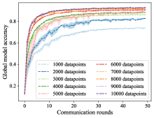
(a) Global model accuracy vs. communication rounds.

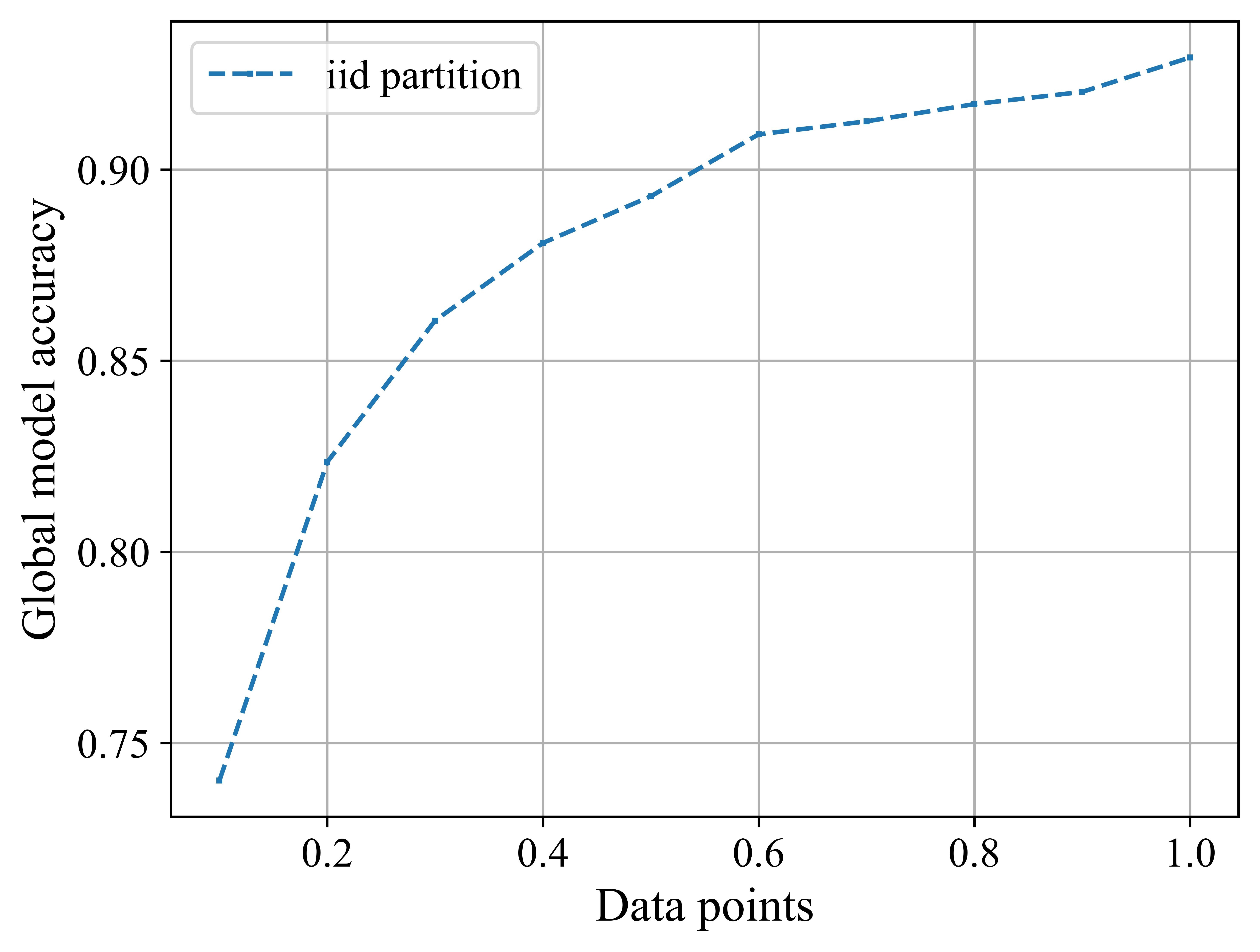
(b) Global model accuracy vs. data contribution at round $50$.

Figure 1: Impact of data contribution on global model accuracy.

V-B Impact of Data Contribution Level and Data Quality on Global Model Accuracy

We conduct experiments to validate our technical assumptions. In particular, we study how the clients’ data contribution $\boldsymbol{s}$ and data quality $\boldsymbol{\epsilon}$ affect the global model accuracy.

Impact of data contribution on global model accuracy: Fig. 1 plots how the global model accuracy depends on the clients’ data contribution. In the experiments, each client uses a randomly selected dataset with size $s_{n}\in 10^{4}\cdot\{0.1,0.2,\cdots,1\}$, and we consider clients have clean labels (i.e., $\epsilon_{n}=0$, $\forall n$). We repeat each experiment 5 runs.

In Fig. 1a, we observe that given a communication round (e.g., round $30$), the model accuracy increases in the data contribution levels. Further, we observe in Fig. 1b that the global model accuracy exhibits a concavely-like increasing trend in the clients’ data contribution, which is consistent with Assumption 1. In fact, the study in [39] also revealed an accuracy curve that concavely increases in the clients’ data contributions using the MNIST dataset.

Impact of data quality on global model accuracy: Fig. 2 plots how the global model accuracy changes with clients’ data quality. In the experiments, each client uses all local data for FL training, and the clients’ data quality (i.e., wrong label percentage $\epsilon_{n}$) takes values in $\{0,0.1,0.2,\cdots,0.5\}$. We repeat each experiment 5 times.

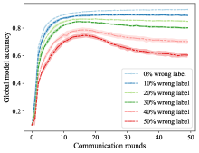
(a) Global model accuracy vs. communication rounds.

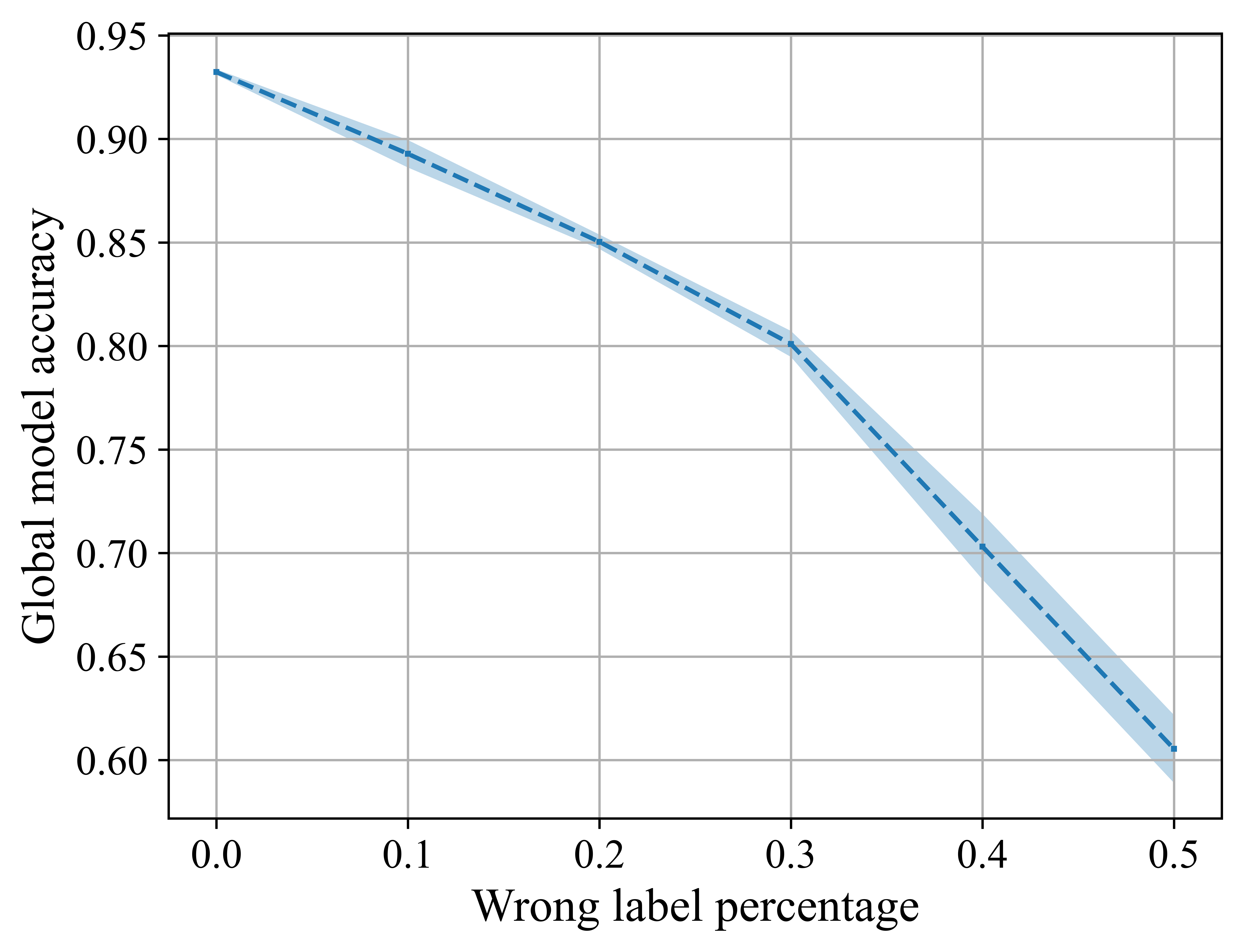
(b) Global model accuracy vs. data quality at round $50$.

Figure 2: Impact of data quality on global model accuracy.

In Fig. 2a, we observe that when clients have relatively high-quality data (e.g., $\epsilon_{n}\in\{0,0.1\}$), the global model accuracy improves as the FL training proceeds. However, when clients’ data quality degrades (e.g., $\epsilon_{n}\geq 0.2$), the global model tends to overfit with more communication rounds. For example, at $\epsilon_{n}=0.5$, the global model accuracy begins to decrease after round $15$. Deep neural networks (e.g., ResNet) tend to overfit to label noise, and overfitting can escalate in FL where clients’ data are private and distributed [44]. This interesting observation bears important implications on how label noise affects FL, and it calls for FL algorithm improvement to mitigate potential overfitting due to label noise.

In Fig. 2b, we observe that the global model accuracy decreases in $\epsilon_{n}$. As clients’ data have more noisy labels, the learned global model would have worse performance. Also, an empirical study in [13] found that label noise can degrade the global model performance. These observations are consistent with Assumption 4.

We summarize the key observations in Figs. 1-2 below:

Observation 1.

(i) The global model accuracy concavely increases in the clients’ data contributions, but it decreases in the wrong label percentage. (ii) The global model tends to overfit when the wrong label percentage is large.

V-C Nash Equilibrium Results

We study how the Nash equilibrium results (calculated by Algorithm 1) depend on the clients’ data quality and privacy sensitivity, followed by the comparison of the four mechanisms (see Eq. (1)-(4)).

Experimental setup: In the experiments, we use a linear privacy cost, i.e., $C_{n}^{\rm pri}(s_{n})=\mu_{n}s_{n}$ [40]. Note that it is empirically infeasible to construct a tabular correspondence between clients’ data contribution $\boldsymbol{s}$ and the global model accuracy $A(\boldsymbol{s},\boldsymbol{\epsilon})$, as this requires FL training for $(D_{n})^{N}=(10^{4})^{5}=10^{20}$ times. Instead, we use a surrogate accuracy function, i.e., $A(\boldsymbol{s},\boldsymbol{\epsilon})=A(\boldsymbol{s},\boldsymbol{0})-\gamma\sum_{n\in\mathcal{N}}\frac{\epsilon_{n}s_{n}}{\sum_{n^{\prime}=1}^{N}s_{n^{\prime}}}$, where $A(\boldsymbol{s},\boldsymbol{0})$ represents the model accuracy when clients have clean labels, and the term $\gamma\sum_{n\in\mathcal{N}}\frac{\epsilon_{n}s_{n}}{\sum_{n^{\prime}=1}^{N}s_{n^{\prime}}}$ characterizes the accuracy loss caused by label noise. The parameter $\gamma$ and the function $A(\boldsymbol{s},\boldsymbol{0})$ are obtained using curve fitting, and in particular, $A(\boldsymbol{s},\boldsymbol{0})=\alpha_{1}\log(\alpha_{2}\sum_{n\in\mathcal{N}}s_{n}+\alpha_{3})+\alpha_{4}\sum_{n\in\mathcal{N}}s_{n}+\alpha_{5}$. Moreover, we use a convex profit function, i.e., $\Pi(A(\boldsymbol{s},\boldsymbol{\epsilon}))=\beta_{1}A^{2}(\boldsymbol{s},\boldsymbol{\epsilon})+\beta_{2}$. It can model the scenario where the total profit increases faster as the global model accuracy improves. For example, one would expect that the profit earned via improving $A$ from $0.9$ to $0.95$ is greater than improving $A$ from $0.7$ to $0.75$.

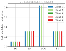
(a) $\epsilon_{1}=\epsilon_{2}=\epsilon_{3}=0$.

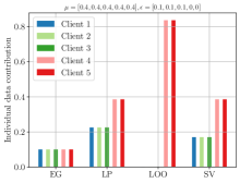
(b) $\epsilon_{1}=\epsilon_{2}=\epsilon_{3}=0.1$.

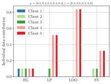
(c) $\epsilon_{1}=\epsilon_{2}=\epsilon_{3}=0.3$.

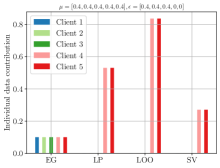
(d) $\epsilon_{1}=\epsilon_{2}=\epsilon_{3}=0.4$.

Figure 3: Impact of data quality on clients’ individual data contributions at Nash equilibrium.

Impact of data quality: We first investigate how data quality affects the clients’ equilibrium data contributions $s_{n}^{*}$, $\forall n$. To this end, we consider that the clients have the same privacy sensitivity, i.e., $\mu_{n}=0.4,\forall n$. Clients have different data qualities, and in the experiments, we set $\epsilon_{4}=\epsilon_{5}=0$. We consider that clients 1-3 have the same wrong label percentage and it takes values in the set $\epsilon_{1}=\epsilon_{2}=\epsilon_{3}\in\{0,0.1,0.2,0.3,0.4,0.5\}$. Fig. 3 plots how clients’ equilibrium $s_{n}^{*}$ depends on $\epsilon_{n}$.

In Fig. 3, we observe that the data contribution of clients 1-3 (weakly) decreases in the wrong label percentage $\epsilon_{n},\forall n\in\{1,2,3\}$, under all mechanisms. This observation is consistent with Theorem 3. Moreover, in Figs. 3b-3d, we find that clients 4-5 use a no smaller data contribution than clients 1-3. This implies that under the above mechanisms, clients with higher-quality data tend to contribute more to FL. We summarize the observation below:

Observation 2.

(i) A client’s equilibrium data contribution decreases in its wrong label percentage. (ii) Clients with higher-quality data contribute more to FL at equilibrium.

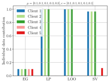
(a) $\mu_{1}=\mu_{2}=\mu_{3}=0.1$.

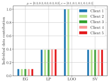
(b) $\mu_{1}=\mu_{2}=\mu_{3}=0.3$.

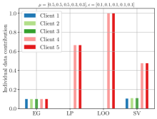
(c) $\mu_{1}=\mu_{2}=\mu_{3}=0.5$.

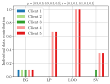
(d) $\mu_{1}=\mu_{2}=\mu_{3}=0.9$.

Figure 4: Impact of privacy sensitivity on clients’ individual data contributions at Nash equilibrium.

Impact of privacy sensitivity: Next, we investigate how clients’ privacy sensitivity affects the equilibrium data contributions. To this end, we consider that clients have the same data quality $\epsilon_{n}=0.1,\forall n$. Clients have different privacy sensitivities, and we set $\mu_{4}=\mu_{5}=0.3$. We consider that clients 1-3 have the same privacy sensitivity and it takes values $\mu_{1}=\mu_{2}=\mu_{3}\in\{0.1,0.3,0.5,0.7,0.9\}$. Fig. 4 plots how clients’ equilibrium $s_{n}^{*}$ changes with $\mu_{n}$.

In Fig. 4, we see that client $n$’s equilibrium data contribution weakly decreases in its privacy sensitivity $\mu_{n},\forall n\in\{1,2,3\}$. This is consistent with Theorem 2. Also, we observe that in Figs. 4c and 4d that clients 4-5 contribute more data than clients 1-3, implying that clients with smaller privacy sensitivity tend to contribute more data at equilibrium. We summarize the observations below:

Observation 3.

(i) A client’s equilibrium data contribution decreases in its privacy sensitivity. (ii) Clients with smaller privacy sensitivity contribute more data at equilibrium.

Comparison of various mechanisms: We now compare the four profit allocation mechanisms in terms of the clients’ equilibrium data contribution.

First, we observe that EG leads to the same equilibrium solutions for all the parameter settings in Fig. 3 and Fig. 4. EG cannot incentivize clients with high-quality data to contribute, as it always equally splits the total profit. Second, when clients have the same data quality (e.g., Fig. 3a), we observe that LP and SV tend to induce similar data contributions among clients, while LOO leads to an imbalanced client contribution (i.e., clients 3-5 do not contribute). Under LOO, once some clients contribute enough data, they can harvest most of the profits and decentivize other clients to contribute data, leading to imbalanced data contribution at equilibrium. Third, when clients differ in data quality (e.g., Figs. 3b,3c,3d), we find that LP, LOO, and SV can incentivize clients with higher-quality data to contribute more data than those with lower-quality data. This demonstrates the effectiveness of the three mechanisms in incentivizing high-quality data contribution in FL. We summarize the above key observations as follows:

Observation 4.

EG cannot incentivize high-quality data contribution, while LP, LOO, and SV incentivize more data contribution from clients with higher-quality data.

To further compare the four mechanisms, we use the equilibrium results (e.g., in Fig. 3 and Fig. 4) to train FL models and present the global model accuracy. Fig. 5 shows how the global model accuracy at equilibrium changes with data quality and privacy sensitivity.

In Fig. 5a and Fig. 5b, we observe that the global model accuracy generally decreases in the wrong label percentage and the privacy sensitivity. As clients have data of lower quality or become more privacy sensitive, they tend to contribute less data, resulting in a worse global model. Furthermore, we find an interesting observation that LOO generally induces the best global model among the four mechanisms. As can be seen in Fig. 3 and Fig. 4, LOO tends to incentivize the most amount of total data contribution albeit from fewer clients with high-quality data (or small privacy sensitivity), leading to the best global model performance. We summarize this observation below.

Observation 5.

LOO tends to outperform EG, LP, and SV in obtaining a better global model at equilibrium.

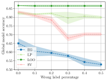
(a) Global model accuracy vs. data quality.

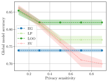
(b) Global model accuracy vs. privacy sensitivity.

Figure 5: Global model accuracy at equilibrium.

VI Discussions

Our paper proposes a first general framework to incentivize data contribution in cross-silo FL using profit allocation. However, some unaddressed challenges merit future study.

Label imbalance: Our work focuses on label noise in FL and how it affects clients’ strategic data contribution. Another important problem in FL is label imbalance, which has drawn extensive recent research attention. However, its impact on clients’ strategic data contribution is poorly understood. We plan to analyze the incentive design in cross-silo FL with label imbalance, and some preliminary numerical results are given in the supplementary material.

Data duplication: We made a widely adopted assumption that the server knows the size of clients’ training dataset $s_{n}$ (i.e., data contribution). In practice, the server may not know this information, and clients can exaggerate their contributions by data duplication/cloning. We conjecture that mechanisms such as LOO and SV can help detect and decentivize malicious data duplication. Under LOO and SV, training models with duplicated data is expected to make little contribution to the global model accuracy, leading to a small contribution index and profit share. This decentivizes data duplication from clients.

Optimal mechanism design: We evaluated our general framework using four widely adopted mechanisms, i.e., EG, LP, LOO, SV. This further motivates the optimal mechanism design that can potentially better incentivize data contribution. It is also interesting to incorporate fairness considerations which are critical in cross-silo settings with medical and financial applications.

VII Conclusion

In cross-silo FL, the clients may not contribute enough data for modeling training due to privacy concerns. To address this issue, we propose a general incentive framework where the profit from the global model can be appropriately allocated to clients to incentivize data contribution. We formulate the interactions among clients as a data contribution game and analyze its equilibrium. We characterize conditions under which an equilibrium exists, and prove that the client’s equilibrium data contribution increases in its data quality but it decreases in its privacy sensitivity. We further conduct numerical experiments using CIFAR-10 and show that the results are consistent with our analysis. Moreover, we find that practical allocation mechanisms such as linearly proportional, leave-one-out, and Shapley-value can incentivize more data contribution from clients with higher-quality data, in which leave-one-out tends to generate the highest global model accuracy.

References

- [1] P. Kairouz and et al., “Advances and open problems in federated learning,” Foundations and Trends® in Machine Learning, vol. 14, no. 1–2, pp. 1–210, 2021.
- [2] C. Huang, J. Huang, and X. Liu, “Cross-silo federated learning: Challenges and opportunities,” arXiv preprint arXiv:2206.12949, 2022.
- [3] [Online]. Available: https://owkin.com/federated-learning/
- [4] [Online]. Available: https://featurecloud.eu/
- [5] [Online]. Available: https://www.lifeinsuranceinternational.com/news/swiss-re-webank/
- [6] M. Noble, A. Bellet, and A. Dieuleveut, “Differentially private federated learning on heterogeneous data,” in International Conference on Artificial Intelligence and Statistics. PMLR, 2022, pp. 10 110–10 145.
- [7] Y. Wen, J. A. Geiping, L. Fowl, M. Goldblum, and T. Goldstein, “Fishing for user data in large-batch federated learning via gradient magnification,” in International Conference on Machine Learning, vol. 162. PMLR, 2022, pp. 23 668–23 684.
- [8] Y. Fraboni, R. Vidal, and M. Lorenzi, “Free-rider attacks on model aggregation in federated learning,” in International Conference on Artificial Intelligence and Statistics. PMLR, 2021, pp. 1846–1854.
- [9] L. Chen, P. Koutris, and A. Kumar, “Towards model-based pricing for machine learning in a data marketplace,” in Proceedings of the 2019 International Conference on Management of Data, 2019, pp. 1535–1552.
- [10] Q. Lin, J. Zhang, J. Liu, K. Ren, J. Lou, J. Liu, L. Xiong, J. Pei, and J. Sun, “Demonstration of dealer: an end-to-end model marketplace with differential privacy,” Proceedings of the VLDB Endowment, vol. 14, no. 12, pp. 2747–2750, 2021.
- [11] X. Wu and H. Yu, “Mars-fl: Enabling competitors to collaborate in federated learning,” IEEE Transactions on Big Data, 2022.
- [12] S. Yang, H. Park, J. Byun, and C. Kim, “Robust federated learning with noisy labels,” IEEE Intelligent Systems, vol. 37, no. 2, pp. 35–43, 2022.
- [13] J. Xu, Z. Chen, T. Q. Quek, and K. F. E. Chong, “Fedcorr: Multi-stage federated learning for label noise correction,” in Proceedings of the IEEE/CVF Conference on Computer Vision and Pattern Recognition, 2022, pp. 10 184–10 193.
- [14] H. Yu, Z. Liu, Y. Liu, T. Chen, M. Cong, X. Weng, D. Niyato, and Q. Yang, “A fairness-aware incentive scheme for federated learning,” in Proceedings of the AAAI/ACM Conference on AI, Ethics, and Society, 2020, pp. 393–399.
- [15] T. Wang, J. Rausch, C. Zhang, R. Jia, and D. Song, “A principled approach to data valuation for federated learning,” in Federated Learning. Springer, 2020, pp. 153–167.
- [16] R. Jia, D. Dao, B. Wang, F. A. Hubis, N. Hynes, N. M. Gürel, B. Li, C. Zhang, D. Song, and C. J. Spanos, “Towards efficient data valuation based on the shapley value,” in The 22nd International Conference on Artificial Intelligence and Statistics. PMLR, 2019, pp. 1167–1176.
- [17] I. Achituve, A. Shamsian, A. Navon, G. Chechik, and E. Fetaya, “Personalized federated learning with gaussian processes,” Advances in Neural Information Processing Systems, vol. 34, pp. 8392–8406, 2021.
- [18] Y. Huang, L. Chu, Z. Zhou, L. Wang, J. Liu, J. Pei, and Y. Zhang, “Personalized cross-silo federated learning on non-iid data,” in Proceedings of the AAAI Conference on Artificial Intelligence, vol. 35, no. 9, 2021, pp. 7865–7873.
- [19] Q. Li, B. He, and D. Song, “Model-contrastive federated learning,” in Proceedings of the IEEE/CVF Conference on Computer Vision and Pattern Recognition, 2021, pp. 10 713–10 722.
- [20] X. Zhang, Y. Li, W. Li, K. Guo, and Y. Shao, “Personalized federated learning via variational bayesian inference,” in International Conference on Machine Learning. PMLR, 2022, pp. 26 293–26 310.
- [21] F. Hanzely, S. Hanzely, S. Horváth, and P. Richtárik, “Lower bounds and optimal algorithms for personalized federated learning,” Advances in Neural Information Processing Systems, vol. 33, pp. 2304–2315, 2020.
- [22] K. Donahue and J. Kleinberg, “Model-sharing games: Analyzing federated learning under voluntary participation,” in Proceedings of the AAAI Conference on Artificial Intelligence, vol. 35, no. 6, 2021, pp. 5303–5311.
- [23] ——, “Optimality and stability in federated learning: A game-theoretic approach,” Advances in Neural Information Processing Systems, vol. 34, pp. 1287–1298, 2021.
- [24] R. H. L. Sim, Y. Zhang, M. C. Chan, and B. K. H. Low, “Collaborative machine learning with incentive-aware model rewards,” in International Conference on Machine Learning. PMLR, 2020, pp. 8927–8936.
- [25] X. Xu, L. Lyu, X. Ma, C. Miao, C. S. Foo, and B. K. H. Low, “Gradient driven rewards to guarantee fairness in collaborative machine learning,” Advances in Neural Information Processing Systems, vol. 34, pp. 16 104–16 117, 2021.
- [26] N. Zhang, Q. Ma, and X. Chen, “Enabling long-term cooperation in cross-silo federated learning: A repeated game perspective,” IEEE Transactions on Mobile Computing, 2022.
- [27] A. Blum, N. Haghtalab, R. L. Phillips, and H. Shao, “One for one, or all for all: Equilibria and optimality of collaboration in federated learning,” in International Conference on Machine Learning. PMLR, 2021, pp. 1005–1014.
- [28] M. J. Osborne and A. Rubinstein, A course in game theory. MIT press, 1994.
- [29] A. Ghorbani, M. Kim, and J. Zou, “A distributional framework for data valuation,” in International Conference on Machine Learning. PMLR, 2020, pp. 3535–3544.
- [30] T. Song, Y. Tong, and S. Wei, “Profit allocation for federated learning,” in 2019 IEEE International Conference on Big Data (Big Data). IEEE, 2019, pp. 2577–2586.
- [31] A. Ghorbani and J. Zou, “Data shapley: Equitable valuation of data for machine learning,” in International Conference on Machine Learning. PMLR, 2019, pp. 2242–2251.
- [32] L. Lyu, X. Xu, Q. Wang, and H. Yu, “Collaborative fairness in federated learning,” in Federated Learning. Springer, 2020, pp. 189–204.
- [33] H. Zhu, J. Xu, S. Liu, and Y. Jin, “Federated learning on non-iid data: A survey,” Neurocomputing, vol. 465, pp. 371–390, 2021.
- [34] M. Li, T. Zhang, Y. Chen, and A. J. Smola, “Efficient mini-batch training for stochastic optimization,” in Proceedings of the 20th ACM SIGKDD international conference on Knowledge discovery and data mining, 2014, pp. 661–670.
- [35] T. Li, A. K. Sahu, M. Zaheer, M. Sanjabi, A. Talwalkar, and V. Smith, “Federated optimization in heterogeneous networks,” Proceedings of Machine Learning and Systems, vol. 2, pp. 429–450, 2020.
- [36] Q. Yang, Y. Liu, T. Chen, and Y. Tong, “Federated machine learning: Concept and applications,” ACM Transactions on Intelligent Systems and Technology (TIST), vol. 10, no. 2, pp. 1–19, 2019.
- [37] H. Gao, A. Xu, and H. Huang, “On the convergence of communication-efficient local sgd for federated learning,” in Proceedings of the AAAI Conference on Artificial Intelligence, vol. 35, no. 9, 2021, pp. 7510–7518.
- [38] T. Roughgarden, “Algorithmic game theory,” Communications of the ACM, vol. 53, no. 7, pp. 78–86, 2010.
- [39] Y. Zhan, P. Li, Z. Qu, D. Zeng, and S. Guo, “A learning-based incentive mechanism for federated learning,” IEEE Internet of Things Journal, vol. 7, no. 7, pp. 6360–6368, 2020.
- [40] S. P. Karimireddy, W. Guo, and M. I. Jordan, “Mechanisms that incentivize data sharing in federated learning,” arXiv preprint arXiv:2207.04557, 2022.
- [41] R. Hu and Y. Gong, “Trading data for learning: Incentive mechanism for on-device federated learning,” in IEEE Global Communications Conference, 2020, pp. 1–6.
- [42] [Online]. Available: https://www.cs.toronto.edu/~kriz/cifar.html
- [43] [Online]. Available: https://pytorch.org/hub/pytorch_vision_resnet/
- [44] X. Fang and M. Ye, “Robust federated learning with noisy and heterogeneous clients,” in Proceedings of the IEEE/CVF Conference on Computer Vision and Pattern Recognition, 2022, pp. 10 072–10 081.