Semi-Supervised Semantic Segmentation Using Unreliable Pseudo-Labels

Abstract

The crux of semi-supervised semantic segmentation is to assign adequate pseudo-labels to the pixels of unlabeled images. A common practice is to select the highly confident predictions as the pseudo ground-truth, but it leads to a problem that most pixels may be left unused due to their unreliability. We argue that every pixel matters to the model training, even its prediction is ambiguous. Intuitively, an unreliable prediction may get confused among the top classes (i.e., those with the highest probabilities), however, it should be confident about the pixel not belonging to the remaining classes. Hence, such a pixel can be convincingly treated as a negative sample to those most unlikely categories. Based on this insight, we develop an effective pipeline to make sufficient use of unlabeled data. Concretely, we separate reliable and unreliable pixels via the entropy of predictions, push each unreliable pixel to a category-wise queue that consists of negative samples, and manage to train the model with all candidate pixels. Considering the training evolution, where the prediction becomes more and more accurate, we adaptively adjust the threshold for the reliable-unreliable partition. Experimental results on various benchmarks and training settings demonstrate the superiority of our approach over the state-of-the-art alternatives.

1 Introduction

Figure 1: Category-wise performance and statistics on number of pixels with reliable and unreliable predictions. Model is trained using $732$ labeled images on PASCAL VOC 2012 [14] and evaluated on the remaining $9,850$ images.

Semantic segmentation is a fundamental task in the computer vision field, and has been significantly advanced along with the rise of deep neural networks [29, 35, 46, 5]. Existing supervised approaches rely on large-scale annotated data, which can be too costly to acquire in practice. To alleviate this problem, many attempts [43, 9, 4, 1, 15, 33, 21, 48] have been made towards semi-supervised semantic segmentation, which learns a model with only a few labeled samples and numerous unlabeled ones. Under such a setting, how to adequately leverage the unlabeled data becomes critical.

A typical solution is to assign pseudo-labels to the pixels without annotations. Concretely, given an unlabeled image, prior arts [27, 41] borrow predictions from the model trained on labeled data, and use the pixel-wise prediction as the “ground-truth” to in turn boost the supervised model. To mitigate the problem of confirmation bias [2], where the model may suffer from incorrect pseudo-labels, existing approaches propose to filter the predictions with their confidence scores [43, 50, 51, 42]. In other words, only the highly confident predictions are used as the pseudo-labels, while the ambiguous ones are discarded.

However, one potential problem caused by only using reliable predictions is that some pixels may never be learned in the entire training process. For example, if the model cannot satisfyingly predict some certain class (e.g., chair in Fig. 1), it becomes difficult to assign accurate pseudo-labels to the pixels regarding such a class, which may lead to insufficient and categorically imbalanced training. From this perspective, we argue that, to make full use of the unlabeled data, every pixel should be properly utilized.

As discussed above, directly using the unreliable predictions as the pseudo-labels will cause the performance degradation [2]. In this paper, we propose an alternative way of Using Unreliable Pseudo-Labels. We call our framework as U²PL. First, we observe that, an unreliable prediction usually gets confused among only a few classes instead of all classes. Taking Fig. 2 as an instance, the pixel with white cross receives similar probabilities on class motorbike and person, but the model is pretty sure about this pixel not belonging to class car and train. Based on this observation, we reconsider the confusing pixels as the negative samples to those unlikely categories. Specifically, after getting the prediction from an unlabeled image, we employ the per-pixel entropy as the metric (see Fig. 2a) to separate all pixels into two groups, i.e., a reliable one and an unreliable one. All reliable predictions are used to derive positive pseudo-labels, while the pixels with unreliable predictions are pushed into a memory bank, which is full of negative samples. To avoid all negative pseudo-labels only coming from a subset of categories, we employ a queue for each category. Such a design ensures that the number of negative samples for each class is balanced. Meanwhile, considering that the quality of pseudo-labels becomes higher along with the model gets more and more accurate, we come up with a strategy to adaptively adjust the threshold for the partition of reliable and unreliable pixels.

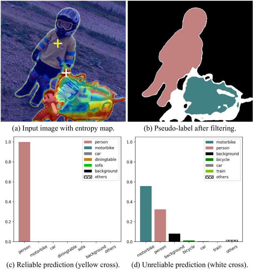
Figure 2: Illustration on unreliable pseudo-labels. (a) Pixel-wise entropy predicted from an unlabeled image, where low-entropy pixels and high-entropy pixels indicate reliable and unreliable predictions, respectively. (b) Pixel-wise pseudo-labels from reliable predictions only, where pixels within the white region are not assigned a pseudo-label. (c) Category-wise probability of a reliable prediction (i.e., the yellow cross), which is confident enough for supervising the class person. (d) Category-wise probability of an unreliable prediction (i.e., the white cross), which hovers between motorbike and person, yet is confident enough of not belonging to car and train.

We evaluate the proposed U²PL on PASCAL VOC 2012 [14] and Cityscapes [10] under a wide range of training settings, where our approach surpasses the state-of-the-art competitors. Furthermore, through visualizing the segmentation results, we find that our method achieves much better performance on those ambiguous regions (e.g., the border between different objects), thanks to our adequate use of the unreliable pseudo-labels.

2 Related Work

Semi-Supervised Learning has two typical paradigms: consistency regularization [3, 33, 15, 36, 42] and entropy minimization [16, 4]. Recently, a more intuitive but effective framework: self-training [27], has become the mainstream. Several methods [15, 44, 43] utilize strong data augmentation such as CutOut [13], CutMix [45], and ClassMix [31] based on self-training. However, these methods do not pay much attention to the characteristics of semantic segmentation, while our method focuses on those unreliable pixels which will be filtered out by most of self-training based methods [44, 43, 34].

Pseudo-Labeling is applied to prevent overfitting to incorrect pseudo-labels when generating predictions of input images from the teacher network [27, 2]. FixMatch [37] utilizes a confidence threshold to select reliable pseudo-labels. UPS [34], a method based on FixMatch [37], takes model uncertainty and data uncertainty into consideration. However, in semi-supervised semantic segmentation, our experiments show including unreliable pixels into training can boost performance.

Model Uncertainty in computer vision is mostly measured by Bayesian deep learning approaches [12, 23, 30]. In our settings, we do not focus on how to measure uncertainty. We simply use the entropy of pixel-wise probability distribution to be the metric.

Contrastive Learning is applied by many successful works in self-supervised learning [7, 8, 17]. In semantic segmentation, contrastive learning has become a promising new paradigm [28, 40, 47, 1, 49]. However, these methods ignore the common false negative samples in semi-supervised segmentation, and unreliable pixels may be wrongly pushed away in contrastive loss. Discriminating the unlikely categories of unreliable pixels can addresses this problem.

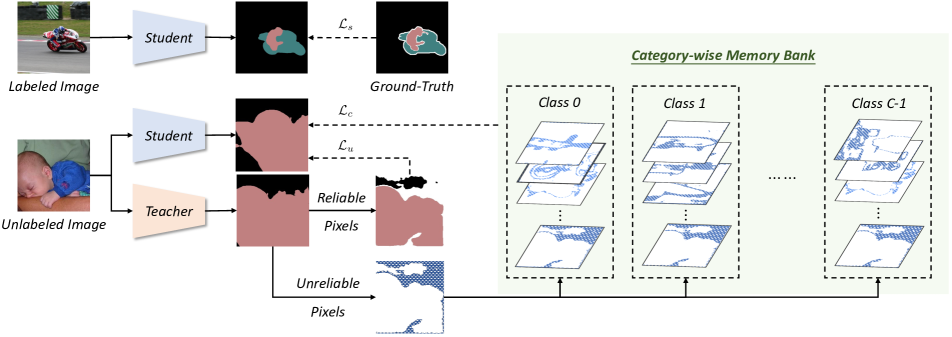
Figure 3: An overview of our proposed U²PL method. U²PL contains a student network and a teacher network, where the teacher is momentum-updated with the student. Labeled data is directly fed into the student network for supervised training. Given an unlabeled image, we first use the teacher model to make a prediction, and then separate the pixels into reliable ones and unreliable ones based on their entropy. Such a process is formulated as Eq. 6. The reliable predictions are directly used as the pseudo-labels to advise the student, while each unreliable prediction is pushed into a category-wise memory bank. Pixels in each memory bank are regarded as the negative samples to the corresponding class, which is formulated as Eq. 4.

Negative Learning aims at decreasing the risk of incorrect information by lowering the probability of negative samples [24, 39, 34, 25], but those negative samples are selected with high confidence. In other words, these methods still utilizes pixels with reliable predictions. By contrast, we propose to make sufficient use of those unreliable predictions for learning instead of filtering them out.

3 Method

In this section, we establish our problem mathematically and give an overview of our proposed method in Sec. 3.1 first. Our strategies about filtering reliable pseudo-labels are introduced in Sec. 3.2. Finally, we describe how to use unreliable pseudo-labels in Sec. 3.3.

3.1 Overview

Given a labeled set $\mathcal{D}_{l}=\left\{(\mathbf{x}_{i}^{l},\mathbf{y}_{i}^{l})\right\}_{i=1}^{N_{l}}$ and a much larger unlabeled set $\mathcal{D}_{u}=\left\{\mathbf{x}_{i}^{u}\right\}_{i=1}^{N_{u}}$, our goal is to train a semantic segmentation model by leveraging both a large amount of unlabeled data and a smaller set of labeled data.

Fig. 3 gives an overview of U²PL, which follows the typical self-training framework with two models of the same architecture, named teacher and student respectively. The two models differ only when updating their weights. The student model’s weights $\theta_{s}$ are updated consistent with the common practice while the teacher model’s weights $\theta_{t}$ are exponential moving average (EMA) updated by the student model’s weights. Each model consists of a CNN-based encoder $h$, a decoder with a segmentation head $f$, and a representation head $g$. At each training step, we equally sample $B$ labeled images $\mathcal{B}_{l}$ and $B$ unlabeled images $\mathcal{B}_{u}$. For every labeled image, our goal is to minimize the standard cross-entropy loss in Eq. 2. As for each unlabeled image, we first take it into the teacher model and get predictions. Then, based on pixel-level entropy, we ignore unreliable pixel-level pseudo-labels when computing unsupervised loss in Eq. 3. This part will be introduced in section Sec. 3.2 in detail. Finally, we use the contrastive loss to make full use of the unreliable pixels excluded in the unsupervised loss, which will be introduced in Sec. 3.3.

Our optimization target is to minimize the overall loss, which can be formulated as:

$$\mathcal{L}=\mathcal{L}_{s}+\lambda_{u}\mathcal{L}_{u}+\lambda_{c}\mathcal{L}_{c},$$ (1)

where $\mathcal{L}_{s}$ and $\mathcal{L}_{u}$ represent supervised loss and unsupervised loss applied on labeled images and unlabeled images respectively, and $\mathcal{L}_{c}$ is the contrastive loss to make full use of unreliable pseudo-labels. $\lambda_{u}$ and $\lambda_{c}$ are weights of unsupervised loss and contrastive loss respectively. Both $\mathcal{L}_{s}$ and $\mathcal{L}_{u}$ are cross-entropy (CE) loss:

$$\mathcal{L}_{s}=\frac{1}{|\mathcal{B}_{l}|}\sum_{(\mathbf{x}_{i}^{l},\mathbf{y}_{i}^{l})\in\mathcal{B}_{l}}\ell_{ce}(f\circ h(\mathbf{x}_{i}^{l};\theta),\mathbf{y}_{i}^{l}),$$ (2)

$$\mathcal{L}_{u}=\frac{1}{|\mathcal{B}_{u}|}\sum_{\mathbf{x}_{i}^{u}\in\mathcal{B}_{u}}\ell_{ce}(f\circ h(\mathbf{x}_{i}^{u};\theta),\hat{\mathbf{y}}_{i}^{u}),$$ (3)

where $\mathbf{y}_{i}^{l}$ represents the hand-annotated mask label for the $i$-th labeled image, and $\hat{\mathbf{y}}_{i}^{u}$ is the pseudo-label for the $i$-th unlabeled image. $f\circ h$ is the composition function of $h$ and $f$, which means the images are first fed into $h$ and then $f$ to get segmentation results. $\mathcal{L}_{c}$ is the pixel-level InfoNCE [32] loss defined as:

$$\mathcal{L}_{c}= -\frac{1}{C\times M}\sum_{c=0}^{C-1}\sum_{i=1}^{M}$$ (4)

$$\log\left[\frac{e^{\langle\mathbf{z}_{ci},\mathbf{z}_{ci}^{+}\rangle/\tau}}{e^{\langle\mathbf{z}_{ci},\mathbf{z}_{ci}^{+}\rangle/\tau}+\sum_{j=1}^{N}e^{\langle\mathbf{z}_{ci},\mathbf{z}_{cij}^{-}\rangle/\tau}}\right],$$

where $M$ is the total number of anchor pixels, and $\mathbf{z}_{ci}$ denotes the representation of the $i$-th anchor of class $c$. Each anchor pixel is followed with a positive sample and $N$ negative samples, whose representations are $\mathbf{z}_{ci}^{+}$ and $\mathbf{z}_{cij}^{-}$ respectively. Note that $\mathbf{z}=g\circ h(\mathbf{x})$ is the output of the representation head. $\langle\cdot,\cdot\rangle$ is the cosine similarity between features from two different pixels, whose range is limited between $-1$ to $1$, hence the need of temperature $\tau$. Following [28], we set $M=50$, $N=256$ and $\tau=0.5$.

3.2 Pseudo-Labeling

To avoid overfitting incorrect pseudo-labels, we utilize entropy of every pixel’s probability distribution to filter high quality pseudo-labels for further supervision. Specifically, we denote $\mathbf{p}_{ij}\in\mathbb{R}^{C}$ as the softmax probabilities generated by the segmentation head of the teacher model for the $i$-th unlabeled image at pixel $j$, where $C$ is the number of classes. Its entropy is computed by:

$$\mathcal{H}(\mathbf{p}_{ij})=-\sum_{c=0}^{C-1}p_{ij}(c)\log p_{ij}(c),$$ (5)

where $p_{ij}(c)$ is the value of $\mathbf{p}_{ij}$ at $c$-th dimension.

Then, we define pixels whose entropy on top $\alpha_{t}$ as unreliable pseudo-labels at training epoch $t$. Such unreliable pseudo-labels are not qualified for supervision. Therefore, we define the pseudo-label for the $i$-th unlabeled image at pixel $j$ as:

$$\hat{y}_{ij}^{u}=\left\{\begin{aligned} &\arg\max_{c}p_{ij}(c),&&\mathrm{if}\ \mathcal{H}(\mathbf{p}_{ij})<\gamma_{t},\\ &\mathrm{ignore},&&\mathrm{otherwise},\end{aligned}\right.$$ (6)

where $\gamma_{t}$ represents the entropy threshold at $t$-th training step. We set $\gamma_{t}$ as the quantile corresponding to $\alpha_{t}$, i.e., $\gamma_{t}$=np.percentile(H.flatten(),100*(1-$\alpha_{t}$)), where H is per-pixel entropy map. We adopt the following adjustment strategies in the pseudo-labeling process for better performance.

Dynamic Partition Adjustment. During the training procedure, the pseudo-labels tend to be reliable gradually. Base on this intuition, we adjust unreliable pixels’ proportion $\alpha_{t}$ with linear strategy every epoch:

$$\alpha_{t}=\alpha_{0}\cdot\left(1-\frac{t}{\mathrm{total\ epoch}}\right),$$ (7)

where $\alpha_{0}$ is the initial proportion and is set to $20\%$, and $t$ is the current training epoch.

Adaptive Weight Adjustment. After obtaining reliable pseudo-labels, we involve them in the unsupervised loss in Eq. 3. The weight $\lambda_{u}$ for this loss is defined as the reciprocal of the percentage of pixels with entropy smaller than threshold $\gamma_{t}$ in the current mini-batch multiplied by a base weight $\eta$:

$$\lambda_{u}=\eta\cdot\frac{|\mathcal{B}_{u}|\times H\times W}{\sum_{i=1}^{|\mathcal{B}_{u}|}\sum_{j=1}^{H\times W}\mathbbm{1}\left[\hat{y}_{ij}^{u}\neq\mathrm{ignore}\right]},$$ (8)

where $\mathbbm{1}(\cdot)$ is the indicator function and $\eta$ is set to $1$.

3.3 Using Unreliable Pseudo-Labels

In semi-supervised learning tasks, discarding unreliable pseudo-labels or reducing their weights is widely used to prevent degradation of model’s performance [50, 43, 37, 41]. We follow this intuition by filtering out unreliable pseudo-labels based on Eq. 6.

However, such contempt for unreliable pseudo-labels may result in information loss. It is obvious that unreliable pseudo-labels can provide information for better discrimination. For example, the white cross in Fig. 2, is a typical unreliable pixel. Its distribution demonstrates model’s uncertainty to distinguish between class person and class motorbike. However, this distribution also demonstrates model’s certainty to not to discriminate this pixel as class car, class train, class bicycle and so on. Such characteristic gives us the main insight to propose our U²PL to use unreliable pseudo-labels for semi-supervised semantic segmentation.

U²PL, with a goal to use the information of unreliable pseudo-labels for better discrimination, coincides with recent popular contrastive learning paradigm in distinguishing representation. But due to the lack of labeled images in semi-supervised semantic segmentation tasks, our U²PL is built on more complicated strategies. U²PL has three components, named anchor pixels, positive candidates and negative candidates. These components are obtained in a sampling manner from certain sets to alleviate huge computational cost. Next, we will introduce how to selecting: (a) anchor pixels (queries); (b) positive samples for each anchor; (c) negative samples for each anchor.

Anchor Pixels. During training, we sample anchor pixels (queries) for each class that appears in the current mini batch. We denote the set of features of all labeled candidate anchor pixels for class $c$ as $\mathcal{A}_{c}^{l}$,

$$\mathcal{A}_{c}^{l}=\left\{\mathbf{z}_{ij}\mid y_{ij}=c,p_{ij}(c)>\delta_{p}\right\},$$ (9)

where $y_{ij}$ is the ground-truth for the $j$-th pixel of labeled image $i$, and $\delta_{p}$ denotes the positive threshold for a particular class and is set to $0.3$ following [28]. $\mathbf{z}_{ij}$ means the representation of the $j$-th pixel of labeled image $i$. For unlabeled data, counterpart $\mathcal{A}_{c}^{u}$ can be computed as:

$$\mathcal{A}_{c}^{u}=\left\{\mathbf{z}_{ij}\mid\hat{y}_{ij}=c,p_{ij}(c)>\delta_{p}\right\}.$$ (10)

It is similar to $\mathcal{A}_{c}^{l}$, and the only difference is that we use pseudo-label $\hat{y}_{ij}$ based on Eq. 6 rather than hand-annotated label, which implies that qualified anchor pixels are reliable, i.e., $\mathcal{H}(\mathbf{p}_{ij})\leq\gamma_{t}$. Therefore, for class $c$, the set of all qualified anchors is

$$\mathcal{A}_{c}=\mathcal{A}_{c}^{l}\cup\mathcal{A}_{c}^{u}.$$ (11)

Positive Samples. The positive sample is the same for all anchors from the same class. It is the center of all possible anchors:

$$\mathbf{z}_{c}^{+}=\frac{1}{|\mathcal{A}_{c}|}\sum_{\mathbf{z}_{c}\in\mathcal{A}_{c}}\mathbf{z}_{c}.$$ (12)

Negative Samples. We define a binary variable $n_{ij}(c)$ to identify whether the $j$-th pixel of image $i$ is qualified to be negative samples of class $c$.

$$n_{ij}(c)=\left\{\begin{aligned} &n_{ij}^{l}(c),&\mathrm{if\ image\ }i\mathrm{\ is\ labeled},\\ &n_{ij}^{u}(c),&\mathrm{otherwise},\end{aligned}\right.$$ (13)

where $n_{ij}^{l}(c)$ and $n_{ij}^{u}(c)$ are indicators of whether the $j$-th pixel of labeled and unlabeled image $i$ is qualified to be negative samples of class $c$ respectively.

For $i$-th labeled image, a qualified negative sample for class $c$ should be: (a) not belonging to class $c$; (b) difficult to distinguish between class $c$ and its ground-truth category. Therefore, we introduce the pixel-level category order $\mathcal{O}_{ij}=\texttt{argsort}(\mathbf{p}_{ij})$. Obviously, we have $\mathcal{O}_{ij}(\arg\max\mathbf{p}_{ij})=0$ and $\mathcal{O}_{ij}(\arg\min\mathbf{p}_{ij})=C-1$.

$$n_{ij}^{l}(c)=\mathbbm{1}\left[y_{ij}\neq c\right]\cdot\mathbbm{1}\left[0\leq\mathcal{O}_{ij}(c)<r_{l}\right],$$ (14)

where $r_{l}$ is the low rank threshold and is set to $3$. The two indicators reflect feature (a) and (b) respectively.

For $i$-th unlabeled image, a qualified negative sample for class $c$ should: (a) be unreliable; (b) probably not belongs to class $c$; (c) not belongs to most unlikely classes. Similarly, we also use $\mathcal{O}_{ij}$ to define $n_{ij}^{u}(c)$:

$$n_{ij}^{u}(c)=\mathbbm{1}\left[\mathcal{H}(\mathbf{p}_{ij})>\gamma_{t}\right]\cdot\mathbbm{1}\left[r_{l}\leq\mathcal{O}_{ij}(c)<r_{h}\right],$$ (15)

where $r_{h}$ is the high rank threshold and is set to $20$. Finally, the set of negative samples of class $c$ is

$$\mathcal{N}_{c}=\left\{\mathbf{z}_{ij}\mid n_{ij}(c)=1\right\}.$$ (16)

Category-wise Memory Bank. Due to the long tail phenomenon of the dataset, negative candidates in some particular categories are extremely limited in a mini-batch. In order to maintain a stable number of negative samples, we use category-wise memory bank $\mathcal{Q}_{c}$ (FIFO queue) to store the negative samples for class $c$.

Finally, the whole process to use unreliable pseudo-labels is shown in Algorithm 1. All features of anchors are attach to gradient, come from student hence, while features of positive and negative samples are from teacher.

1

2Initialize $\mathcal{L}\leftarrow 0$;

3 Sample labeled images $\mathcal{B}_{l}$ and unlabeled images $\mathcal{B}_{u}$;

4

5for $\mathbf{x}_{i}\in\mathcal{B}_{l}\cup\mathcal{B}_{u}$ do

6       Get probabilities: $\mathbf{p}_{i}\leftarrow f\circ h(\mathbf{x}_{i};\theta_{t})$;

7       Get representations: $\mathbf{z}_{i}\leftarrow g\circ h(\mathbf{x}_{i};\theta_{s})$;

8      

9      for $c\leftarrow 0$ to $C-1$ do

10             Get anchors $\mathcal{A}_{c}$ based on Eq. 11;

11             Sample $M$ anchors: $\mathcal{B}_{A}\leftarrow$ sample $(\mathcal{A}_{c})$;

12            

13            Get negatives $\mathcal{N}_{c}$ based on Eq. 16;

14             Push $\mathcal{N}_{c}$ into memory bank $\mathcal{Q}_{c}$;

15             Pop oldest ones out of $\mathcal{Q}_{c}$ if necessary;

16             Sample $N$ negatives: $\mathcal{B}_{N}\leftarrow$ sample $(\mathcal{Q}_{c})$;

17            

18            Get $\mathbf{z}^{+}$ based on Eq. 12;

19            

20            $\mathcal{L}\leftarrow\mathcal{L}+\ell(\mathcal{B}_{A},\mathcal{B}_{N},\mathbf{z}^{+})$ based on Eq. 4;

21            

22       end for

23      

24 end for

25

Output: contrastive loss $\mathcal{L}_{c}\leftarrow\frac{1}{|\mathcal{B}|\times C}\mathcal{L}$

Algorithm 1 Using Unreliable Pseudo-Labels

4 Experiments

4.1 Setup

Datasets. PASCAL VOC 2012 [14] Dataset is a standard semantic segmentation benchmark with 20 semantic classes of objects and 1 class of background. The training set and the validation set include $1,464$ and $1,449$ images respectively. Following [21, 43, 9], we use SBD [18] as the augmented set with $9,118$ additional training images. Since the SBD [18] dataset is coarsely annotated, PseudoSeg [50] takes only the standard $1,464$ images as the whole labeled set, while other methods [9, 21] take all $10,582$ images as candidate labeled data. Therefore, we evaluate our method on both the classic set ($1,464$ candidate labeled images) and the blender set ($10,582$ candidate labeled images). Cityscapes [10], a dataset designed for urban scene understanding, consists of $2,975$ training images with fine-annotated masks and $500$ validation images. For each dataset, we compare U²PL with other methods under $1/2$, $1/4$, $1/8$, and $1/16$ partition protocols.

Table 1: Comparison with state-of-the-art methods on classic PASCAL VOC 2012 val set under different partition protocols. The labeled images are selected from the original VOC train set, which consists of $1,464$ samples in total. The fractions denote the percentage of labeled data used for training, followed by the actual number of images. All the images from SBD [18] are regarded as unlabeled data. “SupOnly” stands for supervised training without using any unlabeled data. † means we reproduce the approach.

Method	1/16 (92)	1/8 (183)	1/4 (366)	1/2 (732)	Full (1464)
SupOnly	45.77	54.92	65.88	71.69	72.50
MT† [38]	51.72	58.93	63.86	69.51	70.96
CutMix† [15]	52.16	63.47	69.46	73.73	76.54
PseudoSeg [50]	57.60	65.50	69.14	72.41	73.23
PC2Seg [48]	57.00	66.28	69.78	73.05	74.15
U2PL (w/ CutMix)	67.98 ($+$15.82)	69.15 ($+$5.68)	73.66 ($+$4.20)	76.16 ($+$2.43)	79.49 ($+$2.95)

Network Structure. We use ResNet-101 [19] pre-trained on ImageNet [11] as the backbone and DeepLabv3+ [6] as the decoder. Both of the segmentation head and the representation head consists of two Conv-BN-ReLU blocks, where both blocks preserve the feature map resolution and the first block halves the number of channels. The segmentation head can be seen as a pixel-level classifier, mapping the $512$ dimensional features output from ASPP module into $C$ classes. The representation head maps the same features into $256$ dimensional representation space.

Evaluation. Following previous methods [21, 48, 33, 15], the images are center cropped into a fixed resolution for PASCAL VOC 2012. For Cityscapes, previous methods apply slide window evaluation, so do we. Then we adopt the mean of Intersection over Union (mIoU) as the metric to evaluate these cropped images. All results are measured on the val set on both Cityscapes [10] and PASCAL VOC 2012 [14]. Ablation studies are conducted on the blender PASCAL VOC 2012 [14] val set under $1/4$ and $1/8$ partition protocol.

Implementation Details. For the training on the blender and classic PASCAL VOC 2012 dataset, we use stochastic gradient descent (SGD) optimizer with initial learning rate $0.001$, weight decay as $0.0001$, crop size as $513\times 513$, batch size as $16$ and training epochs as $80$. For the training on the Cityscapes dataset, we also use stochastic gradient descent (SGD) optimizer with initial learning rate $0.01$, weight decay as $0.0005$, crop size as $769\times 769$, batch size as $16$ and training epochs as $200$. In all experiments, the decoder’s learning rate is ten times that of the backbone. We use the poly scheduling to decay the learning rate during the training process: $lr=lr_{\mathrm{base}}\cdot\left(1-\frac{\mathrm{iter}}{\mathrm{total\ iter}}\right)^{0.9}$.

4.2 Comparison with Existing Alternatives

We compare our method with following recent semi-supervised semantic segmentation methods: Mean Teacher (MT) [38], CCT [33], GCT [22], PseudoSeg [50], CutMix [15], CPS [9], PC²Seg [48], AEL [21]. We re-implement MT [38], CutMix [45] for a fair comparison. For Cityscapes [10], we also reproduce CPS [9] and AEL [21]. All results are equipped with the same network architecture (DeepLabv3+ as decoder and ResNet-101 as encoder). It is important to note the classic PASCAL VOC 2012 Dataset and blender PASCAL VOC 2012 Dataset only differ in training set. Their validation set are the same common one with $1,449$ images.

Table 2: Comparison with state-of-the-art methods on blender PASCAL VOC 2012 val set under different partition protocols. All labeled images are selected from the augmented VOC train set, which consists of $10,582$ samples in total. “SupOnly” stands for supervised training without using any unlabeled data. † means we reproduce the approach.

Method	1/16 (662)	1/8 (1323)	1/4 (2646)	1/2 (5291)
SupOnly	67.87	71.55	75.80	77.13
MT† [38]	70.51	71.53	73.02	76.58
CutMix† [15]	71.66	75.51	77.33	78.21
CCT [33]	71.86	73.68	76.51	77.40
GCT [22]	70.90	73.29	76.66	77.98
CPS [9]	74.48	76.44	77.68	78.64
AEL [21]	77.20	77.57	78.06	80.29
U2PL (w/ CutMix)	77.21 ($+$5.55)	79.01 ($+$3.50)	79.30 ($+$1.97)	80.50 ($+$2.29)

Table 3: Comparison with state-of-the-art methods on Cityscapes val set under different partition protocols. All labeled images are selected from the Cityscapes train set, which consists of $2,975$ samples in total. “SupOnly” stands for supervised training without using any unlabeled data. † means we reproduce the approach.

Method	1/16 (186)	1/8 (372)	1/4 (744)	1/2 (1488)
SupOnly	65.74	72.53	74.43	77.83
MT† [38]	69.03	72.06	74.20	78.15
CutMix† [15]	67.06	71.83	76.36	78.25
CCT [33]	69.32	74.12	75.99	78.10
GCT [22]	66.75	72.66	76.11	78.34
CPS† [9]	69.78	74.31	74.58	76.81
AEL† [21]	74.45	75.55	77.48	79.01
U2PL (w/ CutMix)	70.30 ($+$3.24)	74.37 ($+$2.54)	76.47 ($+$0.11)	79.05 ($+$0.80)
U2PL (w/ AEL)	74.90 ($+$0.45)	76.48 ($+$0.93)	78.51 ($+$1.03)	79.12 ($+$0.11)

Results on classic PASCAL VOC 2012 Dataset. Tab. 1 compares our method with the other state-of-the-art methods on classic PASCAL VOC 2012 Dataset. U²PL outperforms the supervised baseline by $+22.21\%$, $+14.23\%$, $+7.78\%$ and $+4.47\%$ under $1/16$, $1/8$, $1/4$ and $1/2$ partition protocols respectively. For a fair comparison, we only list the methods tested on classic PASCAL VOC 2012. Our method U²PL outperform PC²Seg under all partition protocols by $+10.98\%$, $+2.87\%$, $+3.88\%$ and $+3.11\%$ under $1/16$, $1/8$, $1/4$ and $1/2$ partition protocols respectively. Even under full supervision, our method outperform PC²Seg by $+5.34\%$.

Results on blender PASCAL VOC 2012 Dataset. Tab. 2 shows the comparison results on blender PASCAL VOC 2012 Dataset. Our method U²PL outperforms all the other methods under most partition protocols. Compared with the baseline model (trained with only supervised data), U²PL achieves all improvements of $+9.34\%$, $+7.46\%$, $+3.50\%$ and $+3.37\%$ under $1/16$, $1/8$, $1/4$ and $1/2$ partition protocols respectively. Compared with the existing state-of-the-art methods, U²PL surpasses them under all partition protocols. Especially under $1/8$ protocol and $1/4$ protocol, U²PL outperforms AEL by $+1.44\%$ and $+1.24\%$.

Results on Cityscapes Dataset. Tab. 3 illustrates the comparison results on the Cityscapes val set. U²PL achieves consistent performance gains over the supervised only baseline by $+9.16\%$, $+3.95\%$, $+4.08\%$ and $+1.29\%$ under $1/16$, $1/8$, $1/4$ and $1/2$ partition protocols. U²PL outperforms the existing state-of-the-art method by a notable margin. In particular, U²PL outperforms AEL by $+0.45\%$, $+0.93\%$, $+1.03\%$ and $+0.11\%$ under $1/16$, $1/8$, $1/4$ and $1/2$ partition protocols.

Note that when labeled data is extremely limited, e.g., when we only have $92$ labeled data, our U²PL outperforms previous methods by a large margin ($+10.98\%$ under $1/16$ split for classic PASCAL VOC 2012), proofing the efficiency of using unreliable pseudo-labels.

4.3 Ablation Studies

Effectiveness of Using Unreliable Pseudo-Labels. To prove our core insight, i.e., using unreliable pseudo-labels promotes semi-supervised semantic segmentation, we conduct experiments about selecting negative candidates (Sec. 3.3) with different reliability. Tab. 4 demonstrates the mIoU results on PASCAL VOC 2012 val set. “Unreliable” outperforms other options, proving using unreliable pseudo-labels does help. Appendix B shows the effectiveness of using unreliable pseudo-labels on Cityscapes.

Effectiveness of Probability Rank Threshold. Sec. 3.3 proposes to use probability rank threshold to balance informativeness and confusion caused by unreliable pixels. Tab. 5 provides a verification that such balance promotes the performance. $r_{l}=3$ and $r_{h}=20$ outperform other options by a large margin. When $r_{l}=1$, false negative candidates would not be filtered out, causing the intra-class features of pixels incorrectly distinguished by $\mathcal{L}_{c}$. When $r_{l}=10$, negative candidates tend to become irrelevant with corresponding anchor pixels in semantic, making such discrimination less informative. Sec. D.2 studies PRT and $\alpha_{0}$ on Cityscapes.

Table 4: Ablation study on using pseudo pixels with different reliability, which is measured by the entropy of pixel-wise prediction (see Sec. 3.3). “Unreliable” denotes selecting negative candidates from pixels with top 20% highest entropy scores. “Reliable” denotes the bottom 20% counterpart. “All” denotes sampling regardless of entropy.

	Unreliable	Reliable	All
1/8 (1323)	79.01	77.30	77.40
1/4 (2646)	79.30	77.35	77.57

Table 5: Ablation study on the probability rank threshold, which is described in Sec. 3.3.

$r_{l}$	$r_{h}$	1/8 (1323)	1/4 (2646)
1	3	78.57	79.03
1	20	78.64	79.07
3	10	78.27	78.91
3	20	79.01	79.30
10	20	78.62	78.94

Table 6: Ablation study on the effectiveness of various components in our U²PL, including unsupervised loss $\mathcal{L}_{u}$, contrastive loss $\mathcal{L}_{c}$, category-wise memory bank $\mathcal{Q}_{c}$, Dynamic Partition Adjustment (DPA), Probability Rank Threshold (PRT), and high entropy filtering (Unreliable).

$\mathcal{L}_{c}$	$\mathcal{Q}_{c}$	DPA	PRT	Unreliable	1/4 (2646)
					73.02
✓					77.08
✓	✓		✓	✓	78.49
✓	✓	✓		✓	79.07
✓	✓	✓	✓		77.57
✓	✓	✓	✓	✓	79.30

Table 7: Ablation study on $\alpha_{0}$ in Eq. 7, which controls the initial proportion between reliable and unreliable pixels.

$\alpha_{0}$	40%	30%	20%	10%
1/8 (1323)	76.77	77.34	79.01	77.80
1/4 (2646)	76.92	77.38	79.30	77.95

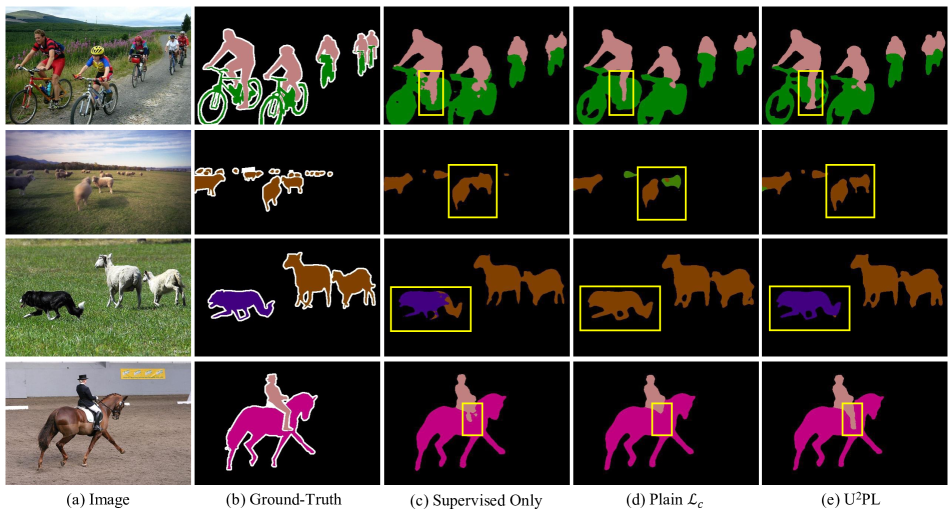
Figure 4: Qualitative results on PASCAL VOC 2012 val set. All models are trained under the $1/4$ partition protocol of blender set, which contains $2,646$ labeled images and $7,396$ unlabeled images. (a) Input images. (b) Hand-annotated labels for the corresponding image. (c) Only labeled images are used for training without any unlabeled data. (d) The vanilla contrastive learning framework, where all pixels are used as negative samples without entropy filtering. (e) Predictions from our U²PL. Yellow rectangles highlight the promotion of segmentation results by adequately using unreliable pseudo-labels.

Effectiveness of Components. We conduct experiments in Tab. 6 to ablate each component of U²PL step by step. For a fair comparison, all the ablations are under 1/4 partition protocol on blender PASCAL VOC 2012 Dataset. Above all, we use no $\mathcal{L}_{c}$ trained model as our baseline, achieving mIoU of $73.02\%$ (MT in Tab. 2). Simply adding $\mathcal{L}_{c}$ without DPA strategy improves the baseline by $+4.06\%$. Category-wise memory bank $\mathcal{Q}_{c}$, along with PRT and high entropy filtering brings an improvement by $+5.47\%$ to baseline. Dynamic Partition Adjustment (DPA) together with high entropy filtering, brings an improvement by $+6.05\%$ to baseline. Note that DPA is a linear adjustment without tuning (refer to Eq. 7), which is simple yet efficient. For Probability Rank Threshold (PRT) component, we set corresponding parameter according to Tab. 5. Without high entropy filtering, the improvement decreased significantly at $+4.55\%$. Finally, when adding all the contribution together, our method achieves state-of-the-art result under $1/4$ partition protocol with mIoU of $79.30\%$. Following this result, we apply these components and corresponding parameters in all experiments on Tab. 2 and Tab. 1.

Ablation Study on Hyper-parameters. We ablate following important parameter for U²PL. Tab. 7 studies the impact of different initial reliable-unreliable partition. This parameter $\alpha_{0}$ have a certain impact on performance. We find $\alpha_{0}=20\%$ achieves the best performance. Small $\alpha_{0}$ will introduce incorrect pseudo labels for supervision, and large $\alpha_{0}$ will make the information of some high-confidence samples underutilized. Other hyper-parameters are studied in Sec. D.1.

4.4 Qualitative Results

Fig. 4 shows the results of different methods on the PASCAL VOC 2012 val set. Benefiting from using unreliable pseudo-labels, U²PL outperforms other methods. Note that using contrastive learning without filtering those unreliable pixels, sometimes does harm to the model (see row 2 and row 4 in Fig. 4), leading to worse results than those when the model is trained only by labeled data.

Furthermore, through visualizing the segmentation results, we find that our method achieves much better performance on those ambiguous regions (e.g., the border between different objects). Such visual difference proves that our method finally makes the reliability of unreliable prediction labels stronger.

5 Conclusion

We propose a semi-supervised semantic segmentation framework U²PL by including unreliable pseudo-labels into training, which outperforms many existing state-of-the-art methods, suggesting our framework provide a new promising paradigm in semi-supervised learning research. Our ablation experiments proves the insight of this work is quite solid. Qualitative result gives a visual proof for its effectiveness, especially the better performance on borders between semantic objects or other ambiguous regions.

The training of our method is time-consuming compared with fully-supervised methods [29, 35, 6, 5, 46], which is a common disadvantage for semi-supervised learning tasks [21, 20, 43, 9, 33, 48]. Due to the extreme lack of labels, the semi-supervised learning frameworks commonly need to pay a price in time for higher accuracy. More in-depth exploration could be conducted on their training optimization in the future.

Appendix

We organize the Appendix as follows. Above all, more details for reproducing the results will be given in Appendix A. Then we will give more results on Cityscapes from two perspectives in Appendix B. We also provide an alternative of contrastive learning to prove our main insight does not only rely on contrastive learning in Appendix C. Besides, ablation studies on both PASCAL VOC 2012 and Cityscapes for more hyper-parameters are given in Appendix D. Finally, visualization on feature space gives a visual proof for the effectiveness of U²PL in Appendix E.

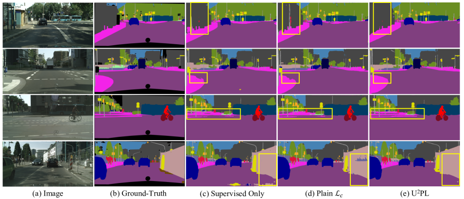
Figure A1: Qualitative results on Cityscapes val set. All models are trained under the $1/2$ partition protocol, which contains $1,488$ labeled images and $1,487$ unlabeled images. (a) Input images. (b) Hand-annotated labels for the corresponding image. (c) Only labeled images are used for training. (d) The vanilla contrastive learning framework, where all pixels are used as negative samples without entropy filtering. (e) Predictions from our U²PL. Yellow rectangles highlight the promotion by adequately using unreliable pseudo-labels.

Appendix A More Details for Reproducibility

For Cityscapes [10], we utilize OHEM which is the same as previous methods [9, 21]. The temperature $\tau$ is set to $0.5$ for both PASCAL VOC 2012 [14] and Cityscapes [10]. We use SGD optimizer for all experiments. For experiments in PASCAL VOC 2012 [14], the initial base learning rate is $0.001$ and the weight decay is $0.0001$. For experiments in Cityscapes [10], the initial base learning rate is $0.01$ and the weight decay is $0.0005$. In our experiments, we find if we train the model only with supervised loss for the initial a few epochs then apply U²PL, it can achieve better performance. We define such epoch as the warm start epoch, and the corresponding warm start epochs for PASCAL VOC 2012 and Cityscapes are $1$ and $20$ respectively.

To prevent overfitting, we apply random cropping, random horizontal flipping, and random scaling with the range of $[0.5,2.0]$ for both PASCAL VOC 2012 [14] and Cityscapes [10] following previous methods [21, 9, 48, 50]. Our memory queue is category-specific. For the background category, the length of the queue is set to be $50,000$. For foreground categories, the length of the queue is all $30,000$. All baselines i.e., “SupOnly”, “MT”, and “CutMix” are re-implemented by ourselves, where the only difference between “MT” and “CutMix” is that the latter applies CutMix [45] augmentation for unlabeled images.

The hyper-parameters used in this work are listed in Tab. A1. Among them, $M,N,\delta_{p}$ are used for contrastive learning, for which we simply follow [28]. $\lambda_{c},\eta,\tau$ are training-related, while $\alpha_{0},r_{l},r_{h}$ are additionally introduced by our U²PL.

Table A1: Summary of hyper-parameters used in U²PL.

Symbol	Description	Default Value
$(M,N)$	contrastive learning settings	(50, 256)
$\delta_{p}$	confidence threshold of positive samples	0.3
$(\lambda_{c},\eta)$	loss weights	(0.1, 1)
$\tau$	loss temperature	0.5
$\alpha_{0}$	initial proportion of unreliable pixels	20%
$(r_{l},r_{h})$	probability rank thresholds	(3, 20)

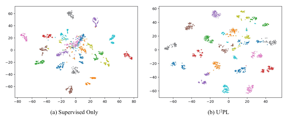
Figure A2: Visualization of the feature spaces learned by our U²PL and its supervised counterpart, using t-SNE [26]. The training set is the 1/4 partition protocol (2646) in blender VOC PASCAL 2012 Dataset.

Appendix B More Results on Cityscapes

Quantitative Results. Tab. A2 demonstrates the mIoU results on Cityscapes val set. “Unreliable” outperforms other options, proving using unreliable pseudo-labels does help. U²PL fully mines the information of all pixels.

Table A2: Ablation study on using pseudo pixels with different reliability, which is measured by the entropy of pixel-wise prediction. “Unreliable” denotes selecting negative candidates from pixels with top 20% highest entropy scores. “Reliable” denotes the bottom 20% counterpart. “All” denotes sampling regardless of entropy. We prove this effectiveness under $1/2$ and $1/4$ partition protocol on Cityscapes val set.

	Unreliable	Reliable	All
1/2 (1488)	79.05	77.19	76.96
1/4 (744)	76.47	75.16	74.51

Qualitative Results. Fig. A1 shows the results of different methods on the Cityscapes val set. Benefiting by using unreliable pseudo-labels, U²PL outperforms other methods. Note that using contrastive learning without filtering those unreliable pixels, sometimes does harm to the model (see the $1$-st row and the $4$-th row in Fig. A1), leading to worse results than those when the model is trained only by labeled data. Such visual difference proves that our method finally makes the reliability of unreliable prediction labels stronger.

Appendix C Alternative of Contrastive Learning

Our proposed U²PL is not limited by contrastive learning. Binary classification is also a sufficient way to use unreliable pseudo-labels, i.e., using binary cross-entropy loss (BCE) $\mathcal{L}_{b}$ other than contrastive loss. For $i$-th anchor $\mathbf{z}_{ci}$ belongs to class $c$, we simply use its negative samples $\{\mathbf{z}_{cij}^{-}\}_{j=1}^{N}$ and positive sample $\mathbf{z}_{c}^{+}$ to compute the BCE loss:

$$\mathcal{L}_{b}=- \frac{1}{C\times M\times N}\sum_{c=0}^{C-1}\sum_{i=1}^{M}\sum_{j=1}^{N}$$ (A1)

$$\log\left[\frac{e^{\langle\mathbf{z}_{ci},\mathbf{z}_{c}^{+}\rangle/\tau}}{e^{\langle\mathbf{z}_{ci},\mathbf{z}_{c}^{+}\rangle/\tau}+e^{\langle\mathbf{z}_{ci},\mathbf{z}_{cij}^{-}\rangle/\tau}}\right],$$

where $C$, $M$, and $N$ are the total number of classes, anchor pixels, and negative samples, respectively. $\langle\cdot,\cdot\rangle$ is the cosine similarity of two features, and $\tau$ represents the temperature.

Tab. A3 and Tab. A4 are results of using unreliable pseudo-labels based on binary classification on Cityscapes [10] and PASCAL VOC 2012 [14] val set respectively. From Tab. A3 and Tab. A4, we can tell that our U²PL is not restricted by contrastive learning, a basic binary classification also does help. On Cityscapes val set, U²PL with $\mathcal{L}_{b}$ can outperforms supervised only baseline by $+3.77\%$, $+0.40\%$, $+1.48\%$, and $+0.53\%$ under $1/16$, $1/8$, $1/4$, and $1/2$ partial protocols. U²PL with $\mathcal{L}_{b}$ can outperforms supervised only baseline by $+7.49\%$, $+5.07\%$, $+3.84\%$, and $+2.67\%$ under $1/16$, $1/8$, $1/4$, and $1/2$ partial protocols on PASCAL VOC 2012 val set. Note that under the $1/4$ partition protocol of blender PASCAL VOC 2012, the bianry classification based U²PL (w/ $\mathcal{L}_{b}$) outperforms the contrastive learning based U²PL (w/ $\mathcal{L}_{c}$) by $+0.34\%$, which proves that contrastive learning is not the only efficient way of using unreliable pseudo-labels.

Table A3: Using unreliable pseudo-labels based on binary classification on Cityscapes val set under different partition protocols.

Method	1/16 (186)	1/8 (372)	1/4 (744)	1/2 (1488)
SupOnly	65.74	72.53	74.43	77.83
MT [38]	69.03	72.06	74.20	78.15
U2PL (w/ $\mathcal{L}_{c}$)	70.30	74.37	76.47	79.05
U2PL (w/ $\mathcal{L}_{b}$)	69.87	72.93	75.91	78.36

Table A4: Using unreliable pseudo-labels based on binary classification on PASCAL VOC 2012 val set under different splits.

Method	1/16 (662)	1/8 (1323)	1/4 (2646)	1/2 (5291)
SupOnly	67.87	71.55	75.80	77.13
MT [38]	70.51	71.53	73.02	76.58
U2PL (w/ $\mathcal{L}_{c}$)	77.21	79.01	79.30	80.50
U2PL (w/ $\mathcal{L}_{b}$)	75.36	76.62	79.64	79.80

Appendix D More Ablation Studies

D.1 More Hyper-parameters on VOC

Base Learning Rate. The impact of the base learning rate is shown in Tab. A5. Results are based on U²PL on blender VOC PASCAL 2012 Dataset. We find that 0.001 outperforms other alternatives.

Temperature. Tab. A6 gives a study on the effect of temperature $\tau$. Temperature $\tau$ plays an important role to adjust the importance to hard samples When $\tau=0.5$, our U²PL achieves best results. Too large or too small of $\tau$ will have an adverse effect on overall performance.

D.2 Ablation Studies on Cityscapes

Probability Rank Threshold. Tab. A7 provides a verification that such balance promotes the performance. $r_{l}=3$ and $r_{h}=20$ outperform other options by a large margin.

Initial Reliable-Unreliable Partition. Tab. A8 studies the impact of different $\alpha_{0}$. When $\alpha_{0}=20\%$, the model achieves the best performance.

Table A5: Ablation study on base learning rate under 1/4 partition protocol (2646) in blender VOC PASCAL 2012 Dataset.

$lr_{\mathrm{base}}$	$10^{-1}$	$10^{-2}$	$10^{-3}$	$10^{-4}$	$10^{-5}$
mIoU	3.49	77.82	79.30	74.58	65.69

Table A6: Ablation study on temperature under 1/4 partition protocol (2646) in blender VOC PASCAL 2012 Dataset.

$\tau$	$10$	$1$	$0.5$	$0.1$	$0.01$
mIoU	78.88	78.91	79.30	79.22	78.78

Table A7: Ablation study on PRT on Cityscapes val set.

$r_{l}$	1	1	3	3	10
$r_{h}$	3	20	10	20	20
1/8 (372)	71.41	72.08	72.60	74.37	72.24
1/4 (744)	76.27	76.04	76.01	76.47	76.18

Table A8: Ablation study on $\alpha_{0}$ on Cityscapes val set.

$\alpha_{0}$	40%	30%	20%	10%
1/8 (372)	72.07	72.93	74.37	71.63
1/4 (744)	75.20	76.08	76.47	76.40

Appendix E Visualization on Feature Space

To have a better understanding of U²PL, we give an illustration on visualization of feature space. Two t-SNE [26] plots are given respectively on the supervised only method and U²PL.

We can observe from Fig. A2 that decision boundaries of features generated by the supervised only method are quite confusing, while U²PL has much more clear ones. This explains why U²PL works from a feature point of view.

References

- [1] Inigo Alonso, Alberto Sabater, David Ferstl, Luis Montesano, and Ana C Murillo. Semi-supervised semantic segmentation with pixel-level contrastive learning from a class-wise memory bank. In Int. Conf. Comput. Vis., 2021.
- [2] Eric Arazo, Diego Ortego, Paul Albert, Noel E O’Connor, and Kevin McGuinness. Pseudo-labeling and confirmation bias in deep semi-supervised learning. In IJCNN, 2020.
- [3] Philip Bachman, Ouais Alsharif, and Doina Precup. Learning with pseudo-ensembles. In Adv. Neural Inform. Process. Syst., 2014.
- [4] Huaian Chen, Yi Jin, Guoqiang Jin, Changan Zhu, and Enhong Chen. Semi-supervised semantic segmentation by improving prediction confidence. IEEE Transactions on Neural Networks and Learning Systems, 13(1), 2021.
- [5] Liang-Chieh Chen, George Papandreou, Iasonas Kokkinos, Kevin Murphy, and Alan L Yuille. Deeplab: Semantic image segmentation with deep convolutional nets, atrous convolution, and fully connected crfs. IEEE Trans. Pattern Anal. Mach. Intell., 40(4):834–848, 2017.
- [6] Liang-Chieh Chen, Yukun Zhu, George Papandreou, Florian Schroff, and Hartwig Adam. Encoder-decoder with atrous separable convolution for semantic image segmentation. In Eur. Conf. Comput. Vis., 2018.
- [7] Ting Chen, Simon Kornblith, Kevin Swersky, Mohammad Norouzi, and Geoffrey Hinton. Big self-supervised models are strong semi-supervised learners. In Adv. Neural Inform. Process. Syst., 2020.
- [8] Xinlei Chen, Saining Xie, and Kaiming He. An empirical study of training self-supervised vision transformers. In Int. Conf. Comput. Vis., 2021.
- [9] Xiaokang Chen, Yuhui Yuan, Gang Zeng, and Jingdong Wang. Semi-supervised semantic segmentation with cross pseudo supervision. In IEEE Conf. Comput. Vis. Pattern Recog., 2021.
- [10] Marius Cordts, Mohamed Omran, Sebastian Ramos, Timo Rehfeld, Markus Enzweiler, Rodrigo Benenson, Uwe Franke, Stefan Roth, and Bernt Schiele. The cityscapes dataset for semantic urban scene understanding. In IEEE Conf. Comput. Vis. Pattern Recog., 2016.
- [11] Jia Deng, Wei Dong, Richard Socher, Li-Jia Li, Kai Li, and Li Fei-Fei. Imagenet: A large-scale hierarchical image database. In IEEE Conf. Comput. Vis. Pattern Recog., 2009.
- [12] Armen Der Kiureghian and Ove Ditlevsen. Aleatory or epistemic? does it matter? Structural Safety, 31(2):105–112, 2009.
- [13] Terrance DeVries and Graham W Taylor. Improved regularization of convolutional neural networks with cutout. arXiv preprint arXiv:1708.04552, 2017.
- [14] Mark Everingham, Luc Van Gool, Christopher KI Williams, John Winn, and Andrew Zisserman. The pascal visual object classes (voc) challenge. International Journal of Computer Vision, 88(2):303–338, 2010.
- [15] Geoff French, Samuli Laine, Timo Aila, Michal Mackiewicz, and Graham Finlayson. Semi-supervised semantic segmentation needs strong, varied perturbations. In Brit. Mach. Vis. Conf., 2020.
- [16] Yves Grandvalet, Yoshua Bengio, et al. Semi-supervised learning by entropy minimization. CAP, 367:281–296, 2005.
- [17] Jean-Bastien Grill, Florian Strub, Florent Altché, Corentin Tallec, Pierre H Richemond, Elena Buchatskaya, Carl Doersch, Bernardo Avila Pires, Zhaohan Daniel Guo, Mohammad Gheshlaghi Azar, et al. Bootstrap your own latent: A new approach to self-supervised learning. arXiv preprint arXiv:2006.07733, 2020.
- [18] Bharath Hariharan, Pablo Arbeláez, Lubomir Bourdev, Subhransu Maji, and Jitendra Malik. Semantic contours from inverse detectors. In Int. Conf. Comput. Vis., 2011.
- [19] Kaiming He, Xiangyu Zhang, Shaoqing Ren, and Jian Sun. Deep residual learning for image recognition. In IEEE Conf. Comput. Vis. Pattern Recog., 2016.
- [20] Ruifei He, Jihan Yang, and Xiaojuan Qi. Re-distributing biased pseudo labels for semi-supervised semantic segmentation: A baseline investigation. In Int. Conf. Comput. Vis., 2021.
- [21] Hanzhe Hu, Fangyun Wei, Han Hu, Qiwei Ye, Jinshi Cui, and Liwei Wang. Semi-supervised semantic segmentation via adaptive equalization learning. In Adv. Neural Inform. Process. Syst., 2021.
- [22] Zhanghan Ke, Di Qiu, Kaican Li, Qiong Yan, and Rynson WH Lau. Guided collaborative training for pixel-wise semi-supervised learning. In Eur. Conf. Comput. Vis., 2020.
- [23] Alex Kendall and Yarin Gal. What uncertainties do we need in bayesian deep learning for computer vision? In Adv. Neural Inform. Process. Syst., 2017.
- [24] Youngdong Kim, Junho Yim, Juseung Yun, and Junmo Kim. Nlnl: Negative learning for noisy labels. In IEEE Conf. Comput. Vis. Pattern Recog., 2019.
- [25] Youngdong Kim, Juseung Yun, Hyounguk Shon, and Junmo Kim. Joint negative and positive learning for noisy labels. In IEEE Conf. Comput. Vis. Pattern Recog., 2021.
- [26] Geoffrey Hinton Laurens Van der Maaten. Visualizing data using t-sne. In JMLR, 2008.
- [27] Dong-Hyun Lee et al. Pseudo-label: The simple and efficient semi-supervised learning method for deep neural networks. In Int. Conf. Mach. Learn., volume 3, page 896, 2013.
- [28] Shikun Liu, Shuaifeng Zhi, Edward Johns, and Andrew J Davison. Bootstrapping semantic segmentation with regional contrast. arXiv preprint arXiv:2104.04465, 2021.
- [29] Jonathan Long, Evan Shelhamer, and Trevor Darrell. Fully convolutional networks for semantic segmentation. In IEEE Conf. Comput. Vis. Pattern Recog., 2015.
- [30] Jishnu Mukhoti and Yarin Gal. Evaluating bayesian deep learning methods for semantic segmentation. arXiv preprint arXiv:1811.12709, 2018.
- [31] Viktor Olsson, Wilhelm Tranheden, Juliano Pinto, and Lennart Svensson. Classmix: Segmentation-based data augmentation for semi-supervised learning. In IEEE Conf. Comput. Vis. Pattern Recog., 2021.
- [32] Aaron van den Oord, Yazhe Li, and Oriol Vinyals. Representation learning with contrastive predictive coding. arXiv preprint arXiv:1807.03748, 2018.
- [33] Yassine Ouali, Céline Hudelot, and Myriam Tami. Semi-supervised semantic segmentation with cross-consistency training. In IEEE Conf. Comput. Vis. Pattern Recog., 2020.
- [34] Mamshad Nayeem Rizve, Kevin Duarte, Yogesh S Rawat, and Mubarak Shah. In defense of pseudo-labeling: An uncertainty-aware pseudo-label selection framework for semi-supervised learning. In Int. Conf. Learn. Represent., 2020.
- [35] Olaf Ronneberger, Philipp Fischer, and Thomas Brox. U-net: Convolutional networks for biomedical image segmentation. In International Conference on Medical Image Computing and Computer Assisted Intervention, pages 234–241. Springer, 2015.
- [36] Mehdi Sajjadi, Mehran Javanmardi, and Tolga Tasdizen. Regularization with stochastic transformations and perturbations for deep semi-supervised learning. In Adv. Neural Inform. Process. Syst., 2016.
- [37] Kihyuk Sohn, David Berthelot, Nicholas Carlini, Zizhao Zhang, Han Zhang, Colin A Raffel, Ekin Dogus Cubuk, Alexey Kurakin, and Chun-Liang Li. Fixmatch: Simplifying semi-supervised learning with consistency and confidence. In Adv. Neural Inform. Process. Syst., 2020.
- [38] Antti Tarvainen and Harri Valpola. Mean teachers are better role models: Weight-averaged consistency targets improve semi-supervised deep learning results. In Adv. Neural Inform. Process. Syst., 2017.
- [39] Hiroki Tokunaga, Brian Kenji Iwana, Yuki Teramoto, Akihiko Yoshizawa, and Ryoma Bise. Negative pseudo labeling using class proportion for semantic segmentation in pathology. In Eur. Conf. Comput. Vis., 2020.
- [40] Wenguan Wang, Tianfei Zhou, Fisher Yu, Jifeng Dai, Ender Konukoglu, and Luc Van Gool. Exploring cross-image pixel contrast for semantic segmentation. In Int. Conf. Comput. Vis., 2021.
- [41] Qizhe Xie, Minh-Thang Luong, Eduard Hovy, and Quoc V Le. Self-training with noisy student improves imagenet classification. In IEEE Conf. Comput. Vis. Pattern Recog., 2020.
- [42] Yi Xu, Lei Shang, Jinxing Ye, Qi Qian, Yu-Feng Li, Baigui Sun, Hao Li, and Rong Jin. Dash: Semi-supervised learning with dynamic thresholding. In Int. Conf. Mach. Learn., 2021.
- [43] Lihe Yang, Wei Zhuo, Lei Qi, Yinghuan Shi, and Yang Gao. St++: Make self-training work better for semi-supervised semantic segmentation. arXiv preprint arXiv:2106.05095, 2021.
- [44] Jianlong Yuan, Yifan Liu, Chunhua Shen, Zhibin Wang, and Hao Li. A simple baseline for semi-supervised semantic segmentation with strong data augmentation. In Int. Conf. Comput. Vis., 2021.
- [45] Sangdoo Yun, Dongyoon Han, Seong Joon Oh, Sanghyuk Chun, Junsuk Choe, and Youngjoon Yoo. Cutmix: Regularization strategy to train strong classifiers with localizable features. In Int. Conf. Comput. Vis., 2019.
- [46] Hengshuang Zhao, Jianping Shi, Xiaojuan Qi, Xiaogang Wang, and Jiaya Jia. Pyramid scene parsing network. In IEEE Conf. Comput. Vis. Pattern Recog., 2017.
- [47] Xiangyun Zhao, Raviteja Vemulapalli, Philip Andrew Mansfield, Boqing Gong, Bradley Green, Lior Shapira, and Ying Wu. Contrastive learning for label efficient semantic segmentation. In Int. Conf. Comput. Vis., 2021.
- [48] Yuanyi Zhong, Bodi Yuan, Hong Wu, Zhiqiang Yuan, Jian Peng, and Yu-Xiong Wang. Pixel contrastive-consistent semi-supervised semantic segmentation. In Int. Conf. Comput. Vis., 2021.
- [49] Yanning Zhou, Hang Xu, Wei Zhang, Bin Gao, and Pheng-Ann Heng. C3-semiseg: Contrastive semi-supervised segmentation via cross-set learning and dynamic class-balancing. In Int. Conf. Comput. Vis., 2021.
- [50] Yuliang Zou, Zizhao Zhang, Han Zhang, Chun-Liang Li, Xiao Bian, Jia-Bin Huang, and Tomas Pfister. Pseudoseg: Designing pseudo labels for semantic segmentation. In Int. Conf. Learn. Represent., 2020.
- [51] Simiao Zuo, Yue Yu, Chen Liang, Haoming Jiang, Siawpeng Er, Chao Zhang, Tuo Zhao, and Hongyuan Zha. Self-training with differentiable teacher. arXiv preprint arXiv:2109.07049, 2021.