NeW CRFs: Neural Window Fully-connected CRFs for Monocular Depth Estimation

Abstract

Estimating the accurate depth from a single image is challenging since it is inherently ambiguous and ill-posed. While recent works design increasingly complicated and powerful networks to directly regress the depth map, we take the path of CRFs optimization. Due to the expensive computation, CRFs are usually performed between neighborhoods rather than the whole graph. To leverage the potential of fully-connected CRFs, we split the input into windows and perform the FC-CRFs optimization within each window, which reduces the computation complexity and makes FC-CRFs feasible. To better capture the relationships between nodes in the graph, we exploit the multi-head attention mechanism to compute a multi-head potential function, which is fed to the networks to output an optimized depth map. Then we build a bottom-up-top-down structure, where this neural window FC-CRFs module serves as the decoder, and a vision transformer serves as the encoder. The experiments demonstrate that our method significantly improves the performance across all metrics on both the KITTI and NYUv2 datasets, compared to previous methods. Furthermore, the proposed method can be directly applied to panorama images and outperforms all previous panorama methods on the MatterPort3D dataset.

1 Introduction

Depth prediction is a classical task in computer vision and is essential for numerous applications such as 3D reconstruction, autonomous driving, and robotics [13, 8, 42, 41]. Such a vision task aims to estimate the depth map from a single color image, which is an ill-posed and inherently ambiguous problem since infinitely many 3D scenes can be projected to the same 2D scene. Therefore, this task is challenging for traditional methods [22, 23, 30], which are usually limited to low-dimension and sparse distances [22], or known and fixed objects [23].

Recently, many works have employed the deep networks to directly regress the depth maps and achieved good performances [6, 17, 1, 18, 7, 2]. Nevertheless, since there are no geometric constraints of multi-view [9, 40, 43] to exploit, the focus of most works is designing more powerful and more complicated networks. This renders this task a difficult fitting problem without the help of other guidance.

In traditional monocular depth estimation, some methods build the energy function from Markov Random Fields (MRFs) or Conditional Random Fields (CRFs) [30, 31, 37]. They exploit the observation cues, such as the texture and position information, along with the last prediction to build the energy function, and then optimize this energy to obtain a depth prediction. This approach is demonstrated to be effective in guiding the estimation of the depth, and is also introduced in some deep methods [20, 11, 29, 38]. However, they are all limited in neighbor CRFs rather than fully-connected CRFs (FC-CRFs) due to the expensive computation, while the fully-connected CRFs capture the relationship between any node in a graph and are much stronger.

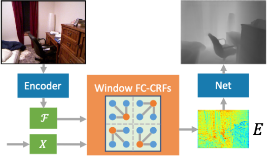
Figure 1: The neural window fully-connected CRFs take image feature $\mathcal{F}$ and upper-level prediction $X$ as input, and compute the fully-connected energy $E$ in each window, which is then fed to the networks to output an optimized depth map.

To address the above challenge, in this work we segment the input to multiple windows, and build the fully-connected CRFs energy within each window, in which way the computation complexity is reduced considerably and the fully-connected CRFs becomes feasible. To capture more relationships between the nodes in the graph, we exploit the multi-head attention mechanism [35] to compute the pairwise potential of the CRFs, and build a new neural CRFs module, as is shown in Figure 1. By employing this neural window FC-CRFs module as decoder, and a vision transformer as encoder, we build a straightforward bottom-up-top-down network to estimate the depth. To make up for the isolation of each window, a window shift action [21] is performed, and the lack of global information in these window FC-CRFs is addressed by aggregating the global features from global average pooling layers [45].

In the experiments, our method is demonstrated to outperform previous methods by a significant margin on both the outdoor dataset, KITTI [8], and the indoor dataset, NYUv2 [32]. Although the state-of-the-art performance on KITTI and NYUv2 has been saturated for a while, our method further reduces the errors considerably on both datasets. Specifically, the Abs-Rel error and the RMS error of KITTI are decreased by $10.3\%$ and $9.8\%$, and that of NYUv2 are decreased by $7.8\%$ and $8.2\%$. Our method now ranks first among all submissions on the KITTI online benchmark. In addition, we evaluate our method on the panorama images. As is well-known, the networks designed for perspective images usually perform poorly on the panorama dataset [34, 36, 14, 33]. Remarkably, our method also sets a new state-of-the-art performance on the panorama dataset, MatterPort3D [3]. This demonstrates that our method can handle the common scenarios in the monocular depth prediction task.

The main contributions of this work are then summarized as follows:

$\bullet$ We split the input image into sub-windows and perform fully-connected CRFs optimization within each window, which reduces the high computation complexity and makes the FC-CRFs feasible.

$\bullet$ We employ the multi-head attention to capture the pairwise relationships in the window FC-CRFs, and embed this neural CRFs module in a network to serve as the decoder.

$\bullet$ We build a new bottom-up-top-down network for monocular depth estimation and show a significant improvement of the monocular depth across all metrics on KITTI, NYUv2, and MatterPort3D datasets.

2 Related Work

2.1 Traditional Monocular Depth Estimation

Prior to the emergence of deep learning, monocular depth estimation is a challenging task. Many published works limit themselves in either estimating 1-D distances of obstacles [22] or limited in several known and fixed objects [23]. Then Saxena et al. [30] claim that local features alone are insufficient to predict the depth of a pixel, and the global context of the whole image needs to be considered to infer the depth. Therefore, they use a discriminatively-trained Markov Random Field (MRF) to incorporate multiscale local and global image features, and model both depths at individual pixels as well as the relation between depths at different pixels. In this way, they infer good depth maps from the monocular cues like colors, pixel positions, occlusion, known object sizes, haze, defocus, etc. Since then, MRFs [31] and CRFs [37] have been well used in monocular depth estimation in traditional methods. However, the traditional approaches still suffer from estimating accurate high-resolution dense depth maps.

2.2 Neural Networks Based Monocular Depth

In monocular depth estimation, neural network based methods have dominated most benchmarks. There are mainly two kinds of approaches for learning the mapping from images to depth maps. The first approach directly regresses the continuous depth map from the aggregation of the information in an image [6, 26, 17, 39, 1, 12, 18, 28]. In this approach, coarse and fine networks are first introduced in [6] and then improved by multi-stage local planar guidance layers in [17]. A bidirectional attention module is proposed in [1] to utilize the feed-forward feature maps and incorporate the global context to filter out ambiguity. Recently, more methods have begun to employ vision transformers to aggregate the information of images [28]. The second approach tries to discretize the depth space and convert the depth prediction to a classification or ordinal regression problem [7, 2]. A spacing-increasing quantization strategy is used in [7] to discretize the depth space more reasonably. Then, an adaptive bins division is computed by the neural networks for better depth quantization. Also, other approaches bring in auxiliary information to help the training of the depth network, such as sparse depth [10] or segmentation information [44, 24, 15, 27]. All these approaches try to directly regress the depth map from the image feature, which falls into a difficult fitting problem. The structures of their networks become increasingly complex. In contrast to these works, we build an energy with the fully-connected CRFs, and then optimize this energy to obtain a high-quality depth map.

2.3 Neural CRFs for Monocular Depth

Since the graph models, like MRFs and CRFs, are effective in traditional depth estimation, some methods try to embed them into neural networks [19, 20, 11, 29, 38]. These methods regard the patches of pixels as nodes and perform the graph optimization. One such approach first uses networks to regress a coarse depth map and then utilizes CRFs to refine it [19], where the post-processing function of CRFs is proven to be effective. However, the CRFs are separated from neural networks. To better combine CRFs and networks, other methods integrate CRFs into the layers of the neural networks and train the whole framework end-to-end [20, 11, 29, 38]. But they are all limited to CRFs rather than fully-connected CRFs due to the high computation complexity.

In this work, different from previous methods, we split the whole graph into multiple sub-windows, such that the fully-connected CRFs become feasible. Also, inspired by recent works in vision transformer[35, 5, 21], we use the multi-head attention mechanism to capture the pairwise relationship in FC-CRFs and propose a neural window fully-connected CRFs module. This module is embedded into the network to play the role of the decoder, such that the whole framework can be trained end-to-end.

3 Neural Window Fully-connected CRFs

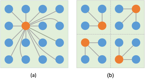
Figure 2: Graph model of fully-connected CRFs and window fully-connected CRFs. In a fully-connected CRFs graph (a), taking the orange node as an example, it is connected to all other nodes in the graph. In a window fully-connected CRFs, however, the orange node is only connected to all other nodes within one window.

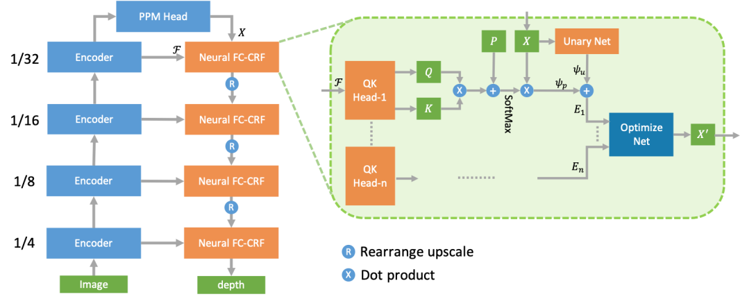
Figure 3: Network structure of the proposed framework. The encoder first extracts the features in four levels. A PPM head aggregates the global and local information and makes the initial prediction $X$ from the top image feature $\mathcal{F}$. Then in each level, the neural window fully-connected CRFs module builds multi-head energy from $X$ and $\mathcal{F}$, and optimizes it to a better prediction $X^{\prime}$. Between each level a rearrange upscale is performed considering the sharpness and network weight.

This section first introduces the window fully-connected CRFs, followed by its integration with neural networks. Afterward, the network structure is displayed, where the neural window FC-CRFs module is embedded into a top-down-bottom-up network to serve as the decoder.

3.1 Fully-connected Conditional Random Fields

In traditional methods, Markov random fields (MRFs) or conditional random fields (CRFs) are leveraged to handle dense prediction tasks such as monocular depth estimation [30] and semantic segmentation [4]. They are shown to be effective in correcting the erroneous predictions based on the information of the current and adjacent nodes. Specifically, in a graph model, these methods favor similar label assignments to nodes that are proximal in space and color.

Thus, in this work we employ CRFs to help the depth prediction. Since the depth prediction of the current pixel is determined by long-range pixels in one image, to increase the receptive field, we use fully-connected CRFs [16] to build the energy. In a graph model, the energy function of the fully-connected CRFs is usually defined as

$$E(\mathbf{x})=\sum_{i}\psi_{u}(x_{i})+\sum_{ij}\psi_{p}(x_{i},x_{j}),$$ (1)

where $x_{i}$ is the predicted value of node $i$, and $j$ denotes all other nodes in the graph. The unary potential function $\psi_{u}$ is computed for each node by the predictor according to the image features.

The pairwise potential function $\psi_{p}$ connects pairs of nodes as

$$\psi_{p}=\mu(x_{i},x_{j})f(x_{i},x_{j})g(I_{i},I_{j})h(p_{i},p_{j}),$$ (2)

where $\mu(x_{i},x_{j})=1$ if $i\neq j$ and $\mu(x_{i},x_{j})=0$ otherwise, $I_{i}$ is the color of node $i$, $p_{i}$ is the position of node $i$. The pairwise potential usually considers the color and position information to enforce some heuristic punishments, which make the predicted values $x_{i},x_{j}$ more reasonable and logical.

In regular CRFs, the pairwise potential only computes the edge connection between the current node and neighboring nodes. In fully-connected CRFs, however, the connections between the current node and any other nodes in a graph need to be computed, as shown in Figure 2 (a).

3.2 Window Fully-connected CRFs

Although the fully-connected CRFs can bring global-range connections, its disadvantage is also obvious. On the one hand, the number of edges connecting all pixels in an image is large, which makes the computation of this kind of pairwise potential quite resource-consuming. On the other hand, the depth of a pixel is usually not determined by distant pixels. Only pixels within some distance need to be considered.

Therefore, in this work we propose the window-based fully-connected CRFs. We segment an image into multiple patch-based windows. Each window includes $N\times N$ image patches, of which each patch is composed of $n\times n$ pixels. In our graph model, each patch rather than each pixel is regarded as one node. All patches within one window are fully-connected with edges, while the patches of different windows are not connected, as displayed in Figure 2 (b). In this case, the computation of pairwise potential only considers the patches within one window, so that the computation complexity is reduced significantly.

Taking an image with $h\times w$ patches as an example, the computation complexity of FC-CRFs and window FC-CRFs for one iteration are

$$\Omega(\text{FC-CRFs})= \ hw\times\Omega(\psi_{u})+hw(hw-1)\times\Omega(\psi_{p})$$ (3)

$$\Omega(\text{Window FC})= \ hw\times\Omega(\psi_{u})+hw(N^{2}-1)\times\Omega(\psi_{p}),$$

where $N$ is the window size, $\Omega(\mu_{u})$ and $\Omega(\mu_{p})$ are the computation complexity of one unary potential and one pairwise potential, respectively.

In the window fully-connected CRFs, all windows are non-overlapped, which means there is no information connection between any windows. The adjacent windows, however, are physically connected. To resolve the isolation of windows, we shift the windows by $(\frac{N}{2},\frac{N}{2})$ patches in the image and calculate the energy function of shifted windows after computing that of the original windows, similar to swin-transformer [21]. In this way, the isolated neighboring pixels are connected in the shifted windows. Hence, each time we calculate the energy function, we calculate two energy functions successively, one for the original windows and the other one for the shifted windows.

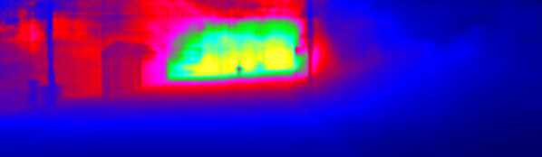
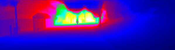
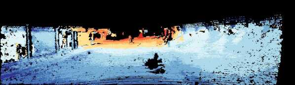
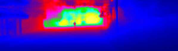
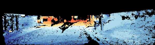
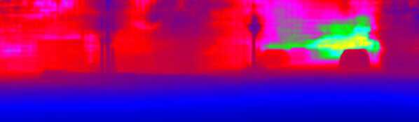
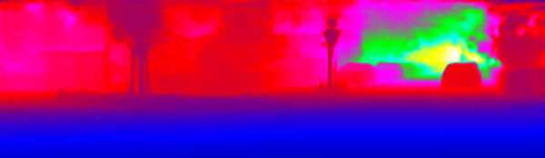
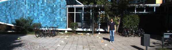
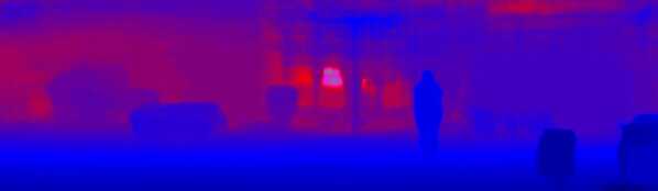
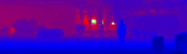
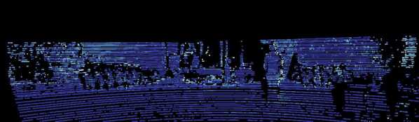
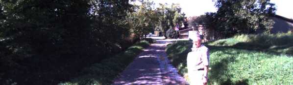
Input image

DORN

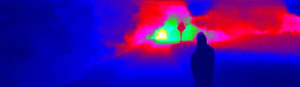
Ours

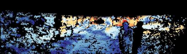
Error map

Figure 4: Qualitative results on the KITTI online benchmark, which are generated by the online server.

3.3 Neural Window FC-CRFs

In traditional CRFs, the unary potential is usually acted by a distribution over the predicted values, e.g.,

$$\psi_{u}(x_{i})=-\log P(x_{i}|I),$$ (4)

where $I$ is the input color image and $P$ is the probability distribution of the value prediction. The pairwise potential is usually computed according to the colors and positions of pixel pairs, e.g.,

$$\psi_{p}(x_{i},x_{j})=\mu(x_{i},x_{j})||x_{i}-x_{j}||e^{-\frac{||I_{i}-I_{j}||}{2\sigma^{2}}}e^{-\frac{||p_{i}-p_{j}||}{2\sigma^{2}}}.$$ (5)

This potential encourages distinct-color and distant pixels to have various value predictions while punishing the value discrepancies in similar-color and adjacent pixels.

These potential functions are designed by hands and cannot be too complicated. Thus they are hard to represent high-dimensional information and describe complex connections. So in this work, we propose to use neural networks to perform the potential functions.

For the unary potential, it is computed from the image features such that it can be directly obtained by the network as

$$\psi_{u}(x_{i})=\theta_{u}(I,x_{i}),$$ (6)

where $\theta$ is the parameters of a unary network.

For the pairwise potential, we realize that it is composed of values of the current node and other nodes, and a weight computed based on the color and position information of the node pairs. So we reformulate it as

$$\psi_{p}(x_{i},x_{j})=w(\mathcal{F}_{i},\mathcal{F}_{j},p_{i},p_{j})||x_{i}-x_{j}||,$$ (7)

where $\mathcal{F}$ is the feature map and $w$ is the weighting function. We calculate the pairwise potential node by node. For each node $i$, we sum all its pairwise potentials and obtain

$$\psi_{p_{i}}=\alpha(\mathcal{F}_{i},\mathcal{F}_{j},p_{i},p_{j})x_{i}+\sum_{j\neq i}\beta(\mathcal{F}_{i},\mathcal{F}_{j},p_{i},p_{j})x_{j},$$ (8)

where $\alpha,\beta$ are the weighting functions and will be computed by the networks.

Inspired by recent works in transformer [35, 5], we calculate a query vector $\mathbf{q}$ and a key vector $\mathbf{k}$ from the feature map of each patch in a window and combine vectors of all patches to matrices $Q$ and $K$. Then we calculate the dot product of matrices $Q$ and $K$ to get the potential weight between any pair, after which the predicted values $X$ are multiplied by the weights to get the final pairwise potential. To introduce the position information, we also add a relative position embedding $P$. Therefore, the equation 8 can be calculated as

$$\psi_{p_{i}}= \ \text{SoftMax}(q\cdot K^{T}+P)\cdot X$$ (9)

$$\sum_{i}\psi_{p_{i}}= \ \text{SoftMax}(Q\cdot K^{T}+P)\cdot X,$$

where $\cdot$ denotes dot production. Thus, the output of the SoftMax gets the weights $\alpha$ and $\beta$ of Equation 8. Therefore, the dot product between $Q$ and $K$ calculates the scores between each node with any other node, which determines the message passing weights with $P$, while the dot product between previous prediction $X$ and the output of the SoftMax performs the message passing.

3.4 Network Structure

Overview.

To embed the neural window fully-connected CRFs into a depth prediction network, we build a bottom-up-top-down structure, where four levels of CRFs optimizations are performed, as is shown in Figure 3. We embed this neural window FC-CRFs module into the network to act as a decoder, which predicts the next-level depth according to the coarse depth and image features. For the encoder, we employ the swin-transformer[21] to extract the features.

For an image with the size of $H\times W$, there are four levels of image patches for the feature extraction encoder and the CRFs optimization decoder, from $4\times 4$ pixels to $32\times 32$ pixels. At each level, $N\times N$ patches make up a window. The window size $N$ is fixed at all levels, so there will be $\frac{H}{4N}\times\frac{W}{4N}$ windows at the bottom level and $\frac{H}{32N}\times\frac{W}{32N}$ windows at the top level.

Global Information Aggregation.

At the top level, to make up for the lack of global information of the window FC-CRFs, we use the pyramid pooling module (PPM) [45] to aggregate the information of the whole image. Similar to [45], we use global averaging pooling of scales $1,2,3,6$ to extract the global information, which is then concatenated with the input feature to map to the top-level prediction $X$ by a convolutional layer.

Neural Window FC-CRFs Module.

In each neural window FC-CRFs block, there are two successive CRFs optimizations, one for regular windows and the other one for shifted windows. To cooperate with the transformer encoder, the window size $N$ is set to $7$, which means each window contains $7\times 7$ patches. The unary potential is computed by a convolutional network and the pairwise potential is computed according to equation 9. In each CRFs optimization, multiple-head $Q$ and $K$ are calculated to obtain multi-head potentials, which can enhance the relationship capturing ability of the energy function. From the top level to the bottom level, a structure of $32,16,8,4$ heads is adopted. Then the energy function is fed into an optimization network composed of two fully-connected layers to output the optimized depth map $X^{\prime}$.

Upscale Module.

After the neural window FC-CRFs decoders at the top three levels, a shuffle operation is performed to rearrange the pixels, by which the image is upscaled from $\frac{h}{2}\times\frac{w}{2}\times d$ to $h\times w\times\frac{d}{4}$. On the one hand, this operation increases the flow to the next level with a larger scale without losing the sharpness like upsampling. On the other hand, this reduces the feature dimension to lighten the subsequent networks.

Training Loss.

Following previous works [17, 2, 18], we use a Scale-Invariant Logarithmic (SILog) loss proposed by [6] to supervise the training. Given the ground-truth depth map, we first calculate the logarithm difference between the predicted depth map and the real depth:

$$\Delta d_{i}=\log\hat{d_{i}}-\log d^{*}_{i},$$ (10)

where $d^{*}_{i}$ is the ground-truth depth value and $\hat{d_{i}}$ is the predicted depth at pixel $i$.

Then for $K$ pixels with valid depth values in an image, the scale-invariant loss is computed as

$$\mathcal{L}=\alpha\sqrt{\frac{1}{K}\sum_{i}\Delta d_{i}^{2}-\frac{\lambda}{K^{2}}(\sum_{i}\Delta d_{i})^{2}},$$ (11)

where $\lambda$ is a variance minimizing factor, and $\alpha$ is a scale constant. In our experiments, $\lambda$ is set to $0.85$ and $\alpha$ is set to $10$ following previous works [17].

Method	cap	Abs Rel $\downarrow$	Sq Rel $\downarrow$	RMSE $\downarrow$	RMSElog $\downarrow$	$\delta<1.25$ $\uparrow$	$\delta<1.25^{2}$ $\uparrow$	$\delta<1.25^{3}$ $\uparrow$
Eigen et al. [6]	0-80m	$0.190$	$1.515$	$7.156$	$0.270$	$0.692$	$0.899$	$0.967$
Liu et al. [20]	0-80m	$0.217$	$-$	$7.046$	$-$	$0.656$	$0.881$	$0.958$
Xu et al. [38]	0-80m	$0.122$	$0.897$	$4.677$	$-$	$0.818$	$0.954$	$0.985$
DORN [7]	0-80m	$0.072$	$0.307$	$2.727$	$0.120$	$0.932$	$0.984$	$0.995$
Yin et al. [39]	0-80m	$0.072$	$-$	$3.258$	$0.117$	$0.938$	$0.990$	$0.998$
BTS [17]	0-80m	$0.059$	$0.241$	$2.756$	$0.096$	$0.956$	$0.993$	$0.998$
PackNet-SAN [10]	0-80m	$0.062$	$-$	$2.888$	$-$	$0.955$	$-$	$-$
Adabin [2]	0-80m	$0.058$	$0.190$	$2.360$	$0.088$	$0.964$	$0.995$	$\mathbf{0.999}$
DPT* [28]	0-80m	$0.062$	$-$	$2.573$	$0.092$	$0.959$	$0.995$	$\mathbf{0.999}$
PWA [18]	0-80m	$0.060$	$0.221$	$2.604$	$0.093$	$0.958$	$0.994$	$\mathbf{0.999}$
Ours	0-80m	$\mathbf{0.052}$	$\mathbf{0.155}$	$\mathbf{2.129}$	$\mathbf{0.079}$	$\mathbf{0.974}$	$\mathbf{0.997}$	$\mathbf{0.999}$

Table 1: Quantitative results on the Eigen split of KITTI dataset. Seven widely used metrics are reported. “Abs Rel” error is the main ranking metric. Note that the “Sq Rel” error is calculated in a different way here. “*” means using additional data for training.

Method	dataset	SILog $\downarrow$	Abs Rel $\downarrow$	Sq Rel $\downarrow$	iRMSE $\downarrow$	RMSE $\downarrow$	$\delta<1.25$ $\uparrow$	$\delta<1.25^{2}$ $\uparrow$	$\delta<1.25^{3}$ $\uparrow$
DORN [7]	val	$12.22$	$11.78$	$3.03$	$11.68$	$3.80$	$0.913$	$0.985$	$0.995$
BTS [17]	val	$10.67$	$7.51$	$1.59$	$8.10$	$3.37$	$0.938$	$0.987$	$0.996$
BA-Full [1]	val	$10.64$	$8.25$	$1.81$	$8.47$	$3.30$	$0.938$	$0.988$	$0.997$
Ours	val	$\mathbf{8.31}$	$\mathbf{5.54}$	$\mathbf{0.89}$	$\mathbf{6.34}$	$\mathbf{2.55}$	$\mathbf{0.968}$	$\mathbf{0.995}$	$\mathbf{0.998}$
DORN [7]	online test	$11.77$	$8.78$	$2.23$	$12.98$	$-$	$-$	$-$	$-$
BTS [17]	online test	$11.67$	$9.04$	$2.21$	$12.23$	$-$	$-$	$-$	$-$
BA-Full [1]	online test	$11.61$	$9.38$	$2.29$	$12.23$	$-$	$-$	$-$	$-$
PackNet-SAN [10]	online test	$11.54$	$9.12$	$2.35$	$12.38$	$-$	$-$	$-$	$-$
PWA [18]	online test	$11.45$	$9.05$	$2.30$	$12.32$	$-$	$-$	$-$	$-$
Ours	online test	$\mathbf{10.39}$	$\mathbf{8.37}$	$\mathbf{1.83}$	$\mathbf{11.03}$	$-$	$-$	$-$	$-$

Table 2: Quantitative results on the official split of KITTI dataset. Eight widely used metrics are reported for the validation set while only four metrics are available from the online evaluation server for the test set. “SILog” error is the main ranking metric. Our method ranks 1st among all submissions on the KITTI depth prediction online benchmark at the submission time of this paper.

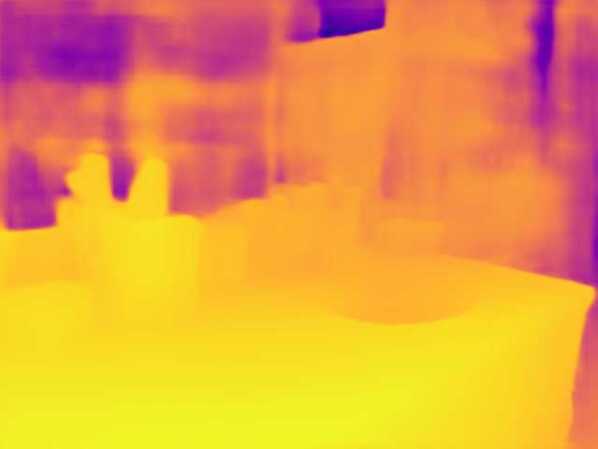
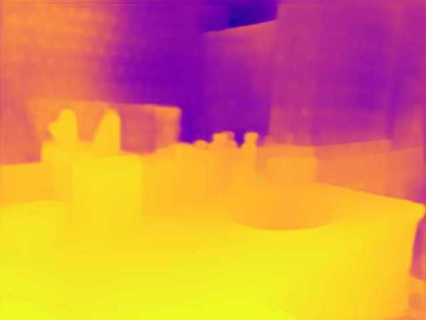
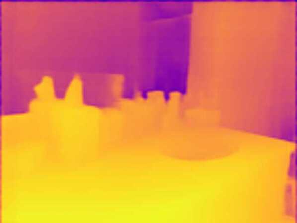
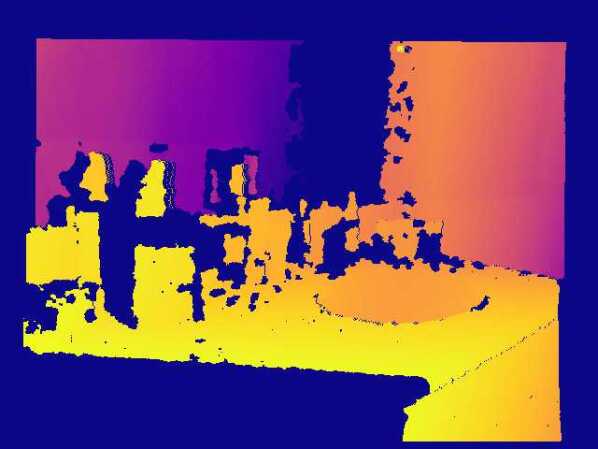
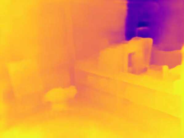
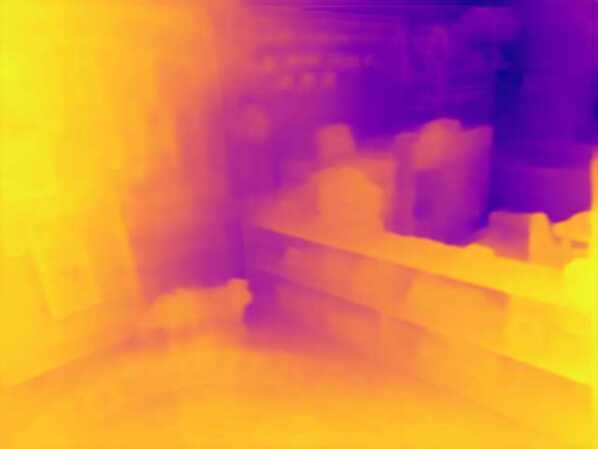
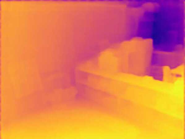
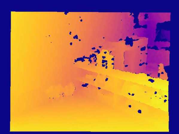
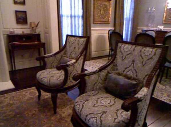
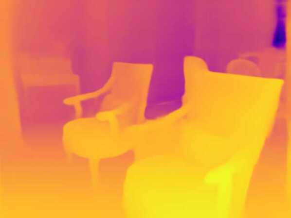
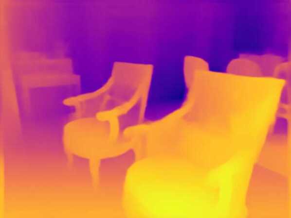
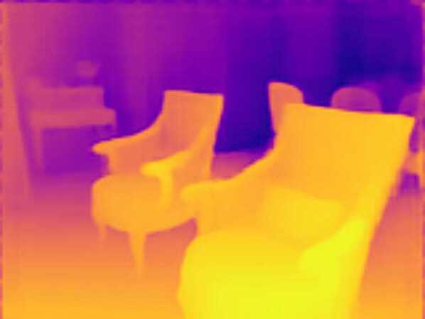
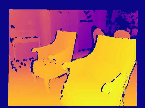
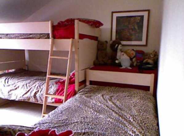
Input image

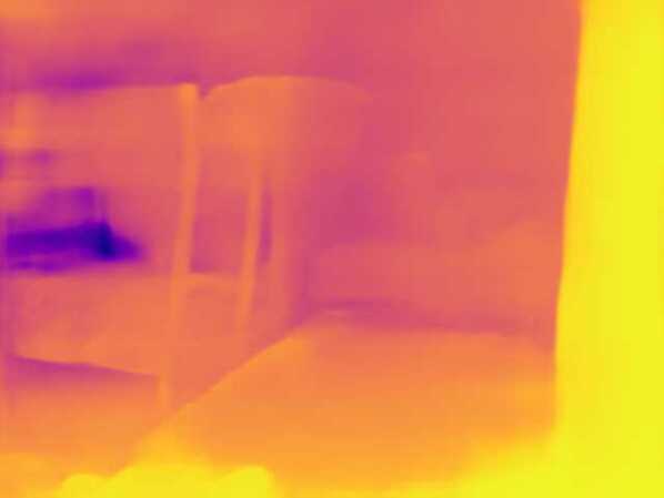
BTS

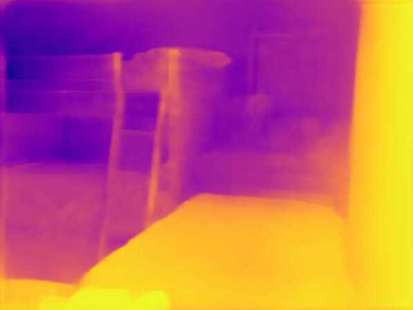
Adabins

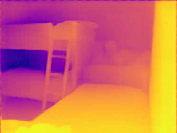
Ours

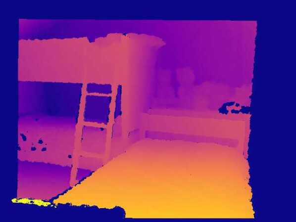
Ground truth

Figure 5: Qualitative results on the NYUv2 dataset.

Method	Abs Rel $\downarrow$	Sq Rel $\downarrow$	RMSE $\downarrow$	RMSElog $\downarrow$	log10 $\downarrow$	$\delta<1.25$ $\uparrow$	$\delta<1.25^{2}$ $\uparrow$	$\delta<1.25^{3}$ $\uparrow$
Liu et al. [20]	$0.230$	$-$	$0.824$	$-$	$0.095$	$0.614$	$0.883$	$0.971$
Xu et al. [38]	$0.125$	$-$	$0.593$	$-$	$0.057$	$0.806$	$0.952$	$0.986$
DORN [7]	$0.115$	$-$	$0.509$	$-$	$0.051$	$0.828$	$0.965$	$0.992$
Yin et al. [39]	$0.108$	$-$	$0.416$	$-$	$0.048$	$0.875$	$0.976$	$0.994$
BTS [17]	$0.110$	$0.066$	$0.392$	$0.142$	$0.047$	$0.885$	$0.978$	$0.994$
DAV [12]	$0.108$	$-$	$0.412$	$-$	$-$	$0.882$	$0.980$	$0.996$
PackNet-SAN* [10]	$0.106$	$-$	$0.393$	$-$	$-$	$0.892$	$0.979$	$0.995$
Adabin [2]	$0.103$	$-$	$0.364$	$-$	$0.044$	$0.903$	$0.984$	$0.997$
DPT* [28]	$0.110$	$-$	$0.357$	$-$	$0.045$	$0.904$	$0.988$	$\mathbf{0.998}$
PWA [18]	$0.105$	$-$	$0.374$	$-$	$0.045$	$0.892$	$0.985$	$0.997$
Ours	$\mathbf{0.095}$	$\mathbf{0.045}$	$\mathbf{0.334}$	$\mathbf{0.119}$	$\mathbf{0.041}$	$\mathbf{0.922}$	$\mathbf{0.992}$	$\mathbf{0.998}$

Table 3: Quantitative results on NYUv2. “Abs Rel” and “RMSE” are the main ranking metrics. “*” means using additional data.

4 Experiments

4.1 Implementation Details

Our work is implemented in Pytorch and experimented on Nvidia GTX 2080 Ti GPUs. The network is optimized end-to-end with the Adam optimizer ($\beta_{1}=0.9$, $\beta_{1}=0.999$). The training runs for $20$ epochs with the batch size of $8$ and the learning rate decreasing from $1\times 10^{-4}$ to $1\times 10^{-5}$. The output depth map of our network is of $\frac{1}{4}\times\frac{1}{4}$ size of the original image, which is then resized to the full resolution.

4.2 Datasets

KITTI dataset. KITTI dataset [8] is the most used benchmark with outdoor scenes captured from a moving vehicle. There are two mainly used splits for monocular depth estimation. One is the training/testing split proposed by Eigen et al. [6] with $23488$ training image pairs and $697$ testing images. The other one is the official split proposed by Geiger et al. [8] with $42949$ training image pairs, $1000$ validation images, and $500$ testing images. For the official split, the ground-truth depth maps for the testing images are withheld by the online evaluation benchmark.

NYUv2 dataset. NYUv2 [32] is an indoor datasets with $120K$ RGB-D videos captured from $464$ indoor scenes. We follow the official training/testing split to evaluate our method, where $249$ scenes are used for training and $654$ images from $215$ scenes are used for testing.

MatterPort3D dataset. To verify the effectiveness of our method on more domains, we also evaluate our method on the panorama images. MatterPort3D [3] is the biggest real-world dataset among all widely used datasets in panorama depth estimation. Following the official split, we use $7829$ images from $61$ houses to train our network and then evaluate the model on the merged set of $957$ validation images and $2014$ testing images. All images are resized to $1024\times 512$ in both training and evaluation.

Method	Abs Rel $\downarrow$	Abs $\downarrow$	RMSE $\downarrow$	RMSElog $\downarrow$	$\delta<1.25$ $\uparrow$	$\delta<1.25^{2}$ $\uparrow$	$\delta<1.25^{3}$ $\uparrow$
OmniDepth [46]	$0.2901$	$0.4838$	$0.7643$	$0.1450$	$0.6830$	$0.8794$	$0.9429$
BiFuse [36]	$0.2048$	$0.3470$	$0.6259$	$0.1134$	$0.8452$	$0.9319$	$0.9632$
SliceNet [25]	$0.1764$	$0.3296$	$0.6133$	$0.1045$	$0.8716$	$0.9483$	$0.9716$
HoHoNet [33]	$0.1488$	$0.2862$	$0.5138$	$0.0871$	$0.8786$	$0.9519$	$0.9771$
UniFuse [14]	$0.1063$	$0.2814$	$0.4941$	$0.0701$	$0.8897$	$0.9623$	$0.9831$
Ours	$\mathbf{0.0906}$	$\mathbf{0.2252}$	$\mathbf{0.4778}$	$\mathbf{0.0638}$	$\mathbf{0.9197}$	$\mathbf{0.9761}$	$\mathbf{0.9909}$
Ours*	$\mathbf{0.0793}$	$\mathbf{0.1970}$	$\mathbf{0.4279}$	$\mathbf{0.0575}$	$\mathbf{0.9376}$	$\mathbf{0.9812}$	$\mathbf{0.9933}$

Table 4: Quantitative results on the Matterport3D dataset. “*” means using additional data for training.

4.3 Evaluations

Evaluation on KITTI. For outdoor scenes, we evaluate our method on the KITTI dataset. We first perform the training and testing on the Eigen split, of which the testing images are available so that the network can be better tuned. The results are reported in Table 1, where we can see that our method outperforms previous methods by a significant margin. Almost all errors are reduced by about $10\%$. Specifically, the “Abs-Rel”, “Sq Rel”, “RMSE” and “RMSE_log” errors are decreased by $10.3\%$, $18.4\%$, $9.8\%$, and $10.2\%$, respectively. Although our method is trained without additional data, it can outperform previous methods trained with additional training data.

We then evaluate our method on the KITTI official split, where the testing images are hidden. The results on the validation set and the testing set are all presented in Table 2. The results of the testing set are cited from the online benchmark and the results of the validation set are cited from BANet [1]. Here we can see that our method reduces the main ranking metric, the SILog error, markedly. Our method now ranks 1st among all submissions on the KITTI depth prediction online server. The colorful visualizations of the predicted depth maps and the error maps generated by the online server are shown in Figure 4. Our method predicts cleaner and smoother depth while maintaining sharper edges of objects, e.g., the edges of the humans.

Evaluation on NYUv2. For indoor scenes, we evaluate our method on the NYUv2 dataset. Since the state-of-the-art performance on NYUv2 dataset has been saturated for a while, some methods have begun to use additional data to pretrain the model and then finetune it on NYUv2 training set [10, 28]. Differently, without any additional data, our method can significantly improve the performance in all metrics, as is shown in Table 3. Specifically, the “Abs Rel” error is reduced to within $0.1$ and the “$\delta<1.25^{2}$” accuracy reaches $99\%$. This emphasizes the contribution of our method in improving the results. The qualitative results in Figure 5 illustrate that our method estimates better depth especially in difficult regions, such as repeated texture, messy environment, and bad light.

Evaluation on MatterPort3D. As is studied in previous works, directly applying a deep network for perspective images to the standard representation of spherical panoramas, i.e., the equirectangular projection, is suboptimal, as it becomes distorted towards the poles [36, 14, 33, 34]. As such, methods in this task try all kinds of ways to convert the panorama images to distortion-free shape, e.g., the cubemap projection [36, 14], the horizontal feature representation [33], and spherical convolutional filters [34]. In comparison to the above-mentioned methods, we directly apply our network designed for perspective images to the panorama images, and outperforms all previous methods, as is presented in Table 4. Specifically, the “Abs Rel” and “Abs” errors are decreased by $14.8\%$ and $20.0\%$.

In addition, we realize that the number of the training set of MatterPort3D is small, so we collect more data in the real world. We use $50K$ images to pretrain the network and then finetune it on the MatterPort3D training set, which results in a better performance, as shown in Table 4. The model pretrained with more data is denoted by “Ours*”. This demonstrates the pretraining with more images can clearly boost the performance in panorama depth estimation.

Setting	Abs Rel	Sq Rel	RMSE	Rlog	$1.25$	$1.25^{2}$
Baseline	$0.069$	$0.256$	$2.610$	$0.103$	$0.947$	$0.993$
Neural CRFs	$0.055$	$0.185$	$2.322$	$0.086$	$0.965$	$0.995$
+ S	$0.054$	$0.174$	$2.297$	$0.084$	$0.968$	$0.996$
+ S + R	$0.054$	$0.168$	$2.271$	$0.083$	$0.970$	$0.996$
+ S + R + P	$0.052$	$0.155$	$2.129$	$0.079$	$0.974$	$0.997$
8, 4, 2, 1	$0.055$	$0.165$	$2.203$	$0.083$	$0.970$	$0.996$
16, 8, 4, 2	$0.054$	$0.162$	$2.172$	$0.081$	$0.972$	$0.997$
32, 16, 8, 4	$0.052$	$0.155$	$2.129$	$0.079$	$0.974$	$0.997$

Table 5: Ablation study on the Eigen split of KITTI dataset. The first six metrics of those used in Table 1 are reported here. “S” refers to window shift, “R” refers to rearrange upscale, and “P” refers to PPM head. The last three rows display the results of using different numbers of heads.

4.4 Abalation Study

To better inspect the effect of each module in our method, we evaluate each component by an ablation study and present the results in Table 5.

Baseline vs. Neural CRFs. To verify the effectiveness of the proposed neural window fully-connected FC-CRFs, we build a baseline model. This model is a well-used UNet structure with the same encoder as ours. In other words, compared to our full method, the PPM head and the rearrange upscale are removed, and the decoder is replaced by the well-used convolutional decoder. Then based on this baseline, we only replace the decoder with our neural window FC-CRFs module, and obtain a noticeable performance improvement as shown in Table 5. The “Abs Rel” error is reduced from $0.069$ to $0.055$, and then to $0.054$ by adding the shift action. This demonstrates the effectiveness of the neural window FC-CRFs in estimating accurate depths.

Rearrange upscale. On top of the basic neural FC-CRFs structure, we add the rearrange upscale module. The performance increment gained from this module is not large, but visually the output depth maps have sharper edges, and the parameters of the network are reduced.

PPM head. The PPM head aggregates the global information, which is lacking in window FC-CRFs. This module can help in some regions that are difficult for estimating with only local information, e.g., the complex texture and the white walls. From the results in Table 5, we see this module contributes to the performance of our framework.

Multi-head energy. The CRFs energy is calculated in a multi-head manner. With more heads, the ability of capturing the pairwise relationship would be stronger but the weight of the network would be heavier. In previous experiments, the numbers of the heads in four levels are set to 32, 16, 8, 4. Here we use fewer heads to see how a lightweight structure performs. From the results in Table 5, fewer heads lead to a small performance decrease.

5 Conclusion

We propose a neural window fully-connected CRFs module to address the monocular depth estimation problem. To solve the expensive computation of FC-CRFs, we split the input into sub-windows and calculate the pairwise potential within each window. To capture the relationships between nodes of the graph, we exploit the multi-head attention to compute a neural potential function. This neural window FC-CRFs module can be directly embedded into a bottom-up-top-down structure and serves as a decoder, which cooperates with a transformer encoder and predicts accurate depth maps. The experiments show that our method significantly outperforms previous methods and sets a new state-of-the-art performance on KITTI, NYUv2, and MatterPort3D datasets.

References

- [1] Shubhra Aich, Jean Marie Uwabeza Vianney, Md Amirul Islam, Mannat Kaur, and Bingbing Liu. Bidirectional attention network for monocular depth estimation. In Proceedings of the IEEE International Conference on Robotics and Automation, pages 11746–11752, 2021.
- [2] Shariq Farooq Bhat, Ibraheem Alhashim, and Peter Wonka. Adabins: Depth estimation using adaptive bins. In Proceedings of the IEEE Conference on Computer Vision and Pattern Recognition, pages 4009–4018, 2021.
- [3] Angel Chang, Angela Dai, Thomas Funkhouser, Maciej Halber, Matthias Niessner, Manolis Savva, Shuran Song, Andy Zeng, and Yinda Zhang. Matterport3d: Learning from rgb-d data in indoor environments. arXiv preprint arXiv:1709.06158, 2017.
- [4] Liang-Chieh Chen, George Papandreou, Iasonas Kokkinos, Kevin Murphy, and Alan L Yuille. Deeplab: Semantic image segmentation with deep convolutional nets, atrous convolution, and fully connected crfs. IEEE Transactions on Pattern Analysis and Machine Intelligence, 40(4):834–848, 2017.
- [5] Alexey Dosovitskiy, Lucas Beyer, Alexander Kolesnikov, Dirk Weissenborn, Xiaohua Zhai, Thomas Unterthiner, Mostafa Dehghani, Matthias Minderer, Georg Heigold, Sylvain Gelly, et al. An image is worth 16x16 words: Transformers for image recognition at scale. In Proceedings of the International Conference on Learning Representations, 2020.
- [6] David Eigen, Christian Puhrsch, and Rob Fergus. Depth map prediction from a single image using a multi-scale deep network. In Advances in Neural Information Processing Systems, pages 2366–2374, 2014.
- [7] Huan Fu, Mingming Gong, Chaohui Wang, Kayhan Batmanghelich, and Dacheng Tao. Deep ordinal regression network for monocular depth estimation. In Proceedings of the IEEE Conference on Computer Vision and Pattern Recognition, pages 2002–2011, 2018.
- [8] Andreas Geiger, Philip Lenz, and Raquel Urtasun. Are we ready for autonomous driving? the kitti vision benchmark suite. In Proceedings of the IEEE Conference on Computer Vision and Pattern Recognition, pages 3354–3361. IEEE, 2012.
- [9] Xiaodong Gu, Weihao Yuan, Zuozhuo Dai, Chengzhou Tang, Siyu Zhu, and Ping Tan. Dro: Deep recurrent optimizer for structure-from-motion. arXiv preprint arXiv:2103.13201, 2021.
- [10] Vitor Guizilini, Rares Ambrus, Wolfram Burgard, and Adrien Gaidon. Sparse auxiliary networks for unified monocular depth prediction and completion. In Proceedings of the IEEE Conference on Computer Vision and Pattern Recognition, pages 11078–11088, 2021.
- [11] Yan Hua and Hu Tian. Depth estimation with convolutional conditional random field network. Neurocomputing, 214:546–554, 2016.
- [12] Lam Huynh, Phong Nguyen-Ha, Jiri Matas, Esa Rahtu, and Janne Heikkilä. Guiding monocular depth estimation using depth-attention volume. In Proceedings of the European Conference on Computer Vision, pages 581–597. Springer, 2020.
- [13] Shahram Izadi, David Kim, Otmar Hilliges, David Molyneaux, Richard Newcombe, Pushmeet Kohli, Jamie Shotton, Steve Hodges, Dustin Freeman, Andrew Davison, et al. Kinectfusion: real-time 3d reconstruction and interaction using a moving depth camera. In Proceedings of the 24th annual ACM symposium on User interface software and technology, pages 559–568, 2011.
- [14] Hualie Jiang, Zhe Sheng, Siyu Zhu, Zilong Dong, and Rui Huang. Unifuse: Unidirectional fusion for 360 panorama depth estimation. IEEE Robotics and Automation Letters, 6(2):1519–1526, 2021.
- [15] Marvin Klingner, Jan-Aike Termöhlen, Jonas Mikolajczyk, and Tim Fingscheidt. Self-supervised monocular depth estimation: Solving the dynamic object problem by semantic guidance. In Proceedings of the European Conference on Computer Vision, pages 582–600. Springer, 2020.
- [16] Philipp Krähenbühl and Vladlen Koltun. Efficient inference in fully connected crfs with gaussian edge potentials. Advances in Neural Information Processing Systems, 24:109–117, 2011.
- [17] Jin Han Lee, Myung-Kyu Han, Dong Wook Ko, and Il Hong Suh. From big to small: Multi-scale local planar guidance for monocular depth estimation. arXiv preprint arXiv:1907.10326, 2019.
- [18] Sihaeng Lee, Janghyeon Lee, Byungju Kim, Eojindl Yi, and Junmo Kim. Patch-wise attention network for monocular depth estimation. In Proceedings of the AAAI Conference on Artificial Intelligence, volume 35, pages 1873–1881, 2021.
- [19] Bo Li, Chunhua Shen, Yuchao Dai, Anton Van Den Hengel, and Mingyi He. Depth and surface normal estimation from monocular images using regression on deep features and hierarchical crfs. In Proceedings of the IEEE Conference on Computer Vision and Pattern Recognition, pages 1119–1127, 2015.
- [20] Fayao Liu, Chunhua Shen, and Guosheng Lin. Deep convolutional neural fields for depth estimation from a single image. In Proceedings of the IEEE Conference on Computer Vision and Pattern Recognition, pages 5162–5170, 2015.
- [21] Ze Liu, Yutong Lin, Yue Cao, Han Hu, Yixuan Wei, Zheng Zhang, Stephen Lin, and Baining Guo. Swin transformer: Hierarchical vision transformer using shifted windows. arXiv preprint arXiv:2103.14030, 2021.
- [22] Jeff Michels, Ashutosh Saxena, and Andrew Y Ng. High speed obstacle avoidance using monocular vision and reinforcement learning. In Proceedings of the International Conference on Machine Learning, pages 593–600, 2005.
- [23] Takaaki Nagai, Takumi Naruse, Masaaki Ikehara, and Akira Kurematsu. Hmm-based surface reconstruction from single images. In Proceedings of the International Conference on Image Processing, volume 2, pages II–II. IEEE, 2002.
- [24] Matthias Ochs, Adrian Kretz, and Rudolf Mester. Sdnet: Semantically guided depth estimation network. In German Conference on Pattern Recognition, pages 288–302. Springer, 2019.
- [25] Giovanni Pintore, Marco Agus, Eva Almansa, Jens Schneider, and Enrico Gobbetti. Slicenet: deep dense depth estimation from a single indoor panorama using a slice-based representation. In Proceedings of the IEEE Conference on Computer Vision and Pattern Recognition, pages 11536–11545, 2021.
- [26] Xiaojuan Qi, Renjie Liao, Zhengzhe Liu, Raquel Urtasun, and Jiaya Jia. Geonet: Geometric neural network for joint depth and surface normal estimation. In Proceedings of the IEEE Conference on Computer Vision and Pattern Recognition, pages 283–291, 2018.
- [27] Siyuan Qiao, Yukun Zhu, Hartwig Adam, Alan Yuille, and Liang-Chieh Chen. Vip-deeplab: Learning visual perception with depth-aware video panoptic segmentation. In Proceedings of the IEEE Conference on Computer Vision and Pattern Recognition, pages 3997–4008, 2021.
- [28] René Ranftl, Alexey Bochkovskiy, and Vladlen Koltun. Vision transformers for dense prediction. In Proceedings of the International Conference on Computer Vision, pages 12179–12188, 2021.
- [29] Elisa Ricci, Wanli Ouyang, Xiaogang Wang, Nicu Sebe, et al. Monocular depth estimation using multi-scale continuous crfs as sequential deep networks. IEEE Transactions on Pattern Analysis and Machine Intelligence, 41(6):1426–1440, 2018.
- [30] Ashutosh Saxena, Sung H Chung, Andrew Y Ng, et al. Learning depth from single monocular images. In Advances in Neural Information Processing Systems, volume 18, pages 1–8, 2005.
- [31] Ashutosh Saxena, Min Sun, and Andrew Y Ng. Make3d: Learning 3d scene structure from a single still image. IEEE Transactions on Pattern Analysis and Machine Intelligence, 31(5):824–840, 2008.
- [32] Nathan Silberman, Derek Hoiem, Pushmeet Kohli, and Rob Fergus. Indoor segmentation and support inference from rgbd images. In Proceedings of the European Conference on Computer Vision, pages 746–760. Springer, 2012.
- [33] Cheng Sun, Min Sun, and Hwann-Tzong Chen. Hohonet: 360 indoor holistic understanding with latent horizontal features. In Proceedings of the IEEE Conference on Computer Vision and Pattern Recognition, pages 2573–2582, 2021.
- [34] Keisuke Tateno, Nassir Navab, and Federico Tombari. Distortion-aware convolutional filters for dense prediction in panoramic images. In Proceedings of the European Conference on Computer Vision, pages 707–722, 2018.
- [35] Ashish Vaswani, Noam Shazeer, Niki Parmar, Jakob Uszkoreit, Llion Jones, Aidan N Gomez, Łukasz Kaiser, and Illia Polosukhin. Attention is all you need. In Advances in Neural Information Processing Systems, pages 5998–6008, 2017.
- [36] Fu-En Wang, Yu-Hsuan Yeh, Min Sun, Wei-Chen Chiu, and Yi-Hsuan Tsai. Bifuse: Monocular 360 depth estimation via bi-projection fusion. In Proceedings of the IEEE Conference on Computer Vision and Pattern Recognition, pages 462–471, 2020.
- [37] Xiaoyan Wang, Chunping Hou, Liangzhou Pu, and Yonghong Hou. A depth estimating method from a single image using foe crf. Multimedia Tools and Applications, 74(21):9491–9506, 2015.
- [38] Dan Xu, Wei Wang, Hao Tang, Hong Liu, Nicu Sebe, and Elisa Ricci. Structured attention guided convolutional neural fields for monocular depth estimation. In Proceedings of the IEEE Conference on Computer Vision and Pattern Recognition, pages 3917–3925, 2018.
- [39] Wei Yin, Yifan Liu, Chunhua Shen, and Youliang Yan. Enforcing geometric constraints of virtual normal for depth prediction. In Proceedings of the IEEE/CVF International Conference on Computer Vision, pages 5684–5693, 2019.
- [40] Weihao Yuan, Rui Fan, Michael Yu Wang, and Qifeng Chen. Mfusenet: Robust depth estimation with learned multiscopic fusion. IEEE Robotics and Automation Letters, 5(2):3113–3120, 2020.
- [41] Weihao Yuan, Kaiyu Hang, Danica Kragic, Michael Y Wang, and Johannes A Stork. End-to-end nonprehensile rearrangement with deep reinforcement learning and simulation-to-reality transfer. Robotics and Autonomous Systems, 119:119–134, 2019.
- [42] Weihao Yuan, Kaiyu Hang, Haoran Song, Danica Kragic, Michael Y Wang, and Johannes A Stork. Reinforcement learning in topology-based representation for human body movement with whole arm manipulation. In Proceedings of the IEEE International Conference on Robotics and Automation, 2019.
- [43] Weihao Yuan, Yazhan Zhang, Bingkun Wu, Siyu Zhu, Ping Tan, Michael Yu Wang, and Qifeng Chen. Stereo matching by self-supervision of multiscopic vision. In Proceedings of the IEEE/RSJ International Conference on Intelligent Robots and Systems, pages 5702–5709. IEEE, 2021.
- [44] Zhenyu Zhang, Zhen Cui, Chunyan Xu, Yan Yan, Nicu Sebe, and Jian Yang. Pattern-affinitive propagation across depth, surface normal and semantic segmentation. In Proceedings of the IEEE Conference on Computer Vision and Pattern Recognition, pages 4106–4115, 2019.
- [45] Hengshuang Zhao, Jianping Shi, Xiaojuan Qi, Xiaogang Wang, and Jiaya Jia. Pyramid scene parsing network. In Proceedings of the IEEE Conference on Computer Vision and Pattern Recognition, pages 2881–2890, 2017.
- [46] Nikolaos Zioulis, Antonis Karakottas, Dimitrios Zarpalas, and Petros Daras. Omnidepth: Dense depth estimation for indoors spherical panoramas. In Proceedings of the European Conference on Computer Vision, pages 448–465, 2018.