Understanding the impact of diffusion of CO in the astrochemical models

Abstract

The mobility of lighter species on the surface of interstellar dust grains plays a crucial role in forming simple through complex molecules. Carbon monoxide is one of the most abundant molecules, its surface diffusion on the grain surface is essential to forming many molecules. Recent laboratory experiments found a diverse range of diffusion barriers for CO on the grain surface, their use can significantly impact the abundance of several molecules. The impact of different diffusion barriers of CO, in the astrochemical models, is studied to understand its effect on the abundance of solid CO and the species for which it is a reactant partner. A gas-grain network is used for three different physical conditions; cold-core and warm-up models with slow and fast heating rates. Two different ratios (0.3 and 0.5) between diffusion and desorption barrier are utilized for all the species. For each physical condition and ratio, six different models are run by varying diffusion barriers of CO. Solid CO abundance for the models with the lowest diffusion barrier yields less than 0.1 % of water ice for cold clouds and a maximum of 0.4 % for slow and fast warm-up models. Also, solid CO₂ in dense clouds is significantly overproduced ($\sim$ 140 % of water). The abundance of H₂CO and CH₃OH showed an opposite trend, and HCOOH, CH₃CHO, NH₂CO, and CH₃COCH₃ are produced in lower quantities for models with low diffusion barriers for CO. Considerable variation in abundance is observed between models with the high and low diffusion barrier. Models with higher diffusion barriers provide a relatively better agreement with the observed abundances when compared with the models having lower diffusion barriers.

Keywords:ISM, molecules, abundances, dust, extinction, astrochemistry

1 Introduction

In the cold ($\sim$ 10 K) and dense interstellar medium (ISM), solid carbon monoxide (CO) is ubiquitous. Its abundance varies from source to source but can be as high as 10^-4 relative to the total hydrogen density. It can form efficiently in the gas phase, which can be depleted on the surface of cold dust grains efficiently (Caselli et al., 1999). On the grain surface, CO can play a significant role in the formation of various molecular species (Garrod et al., 2008). Recent theoretical and laboratory measurements found a considerable variation in the CO diffusion barrier from one measurement to the other. In some cases, it is lower than that is commonly used in astrochemical models. Since surface diffusion is the key to the formation of molecules on the dust grain, therefore, it is important to re-visit the role of CO in the grain surface chemistry.

Molecules that are commonly found in the star-forming regions are partly or almost solely formed on the surface of the bare dust grains or on the water-rich ices that reside on the grains (Herbst & Millar, 2008; Herbst & van Dishoeck, 2009). Interstellar dust grains provide the surface for a reactant to meet with the other and take up the reaction’s excess energy, which makes the reaction possible (Hasegawa et al., 1992). For reaction to occur on the grain surface, reactants need to have sufficient mobility so that they can scan the grain surface in search of a reaction partner. The mobility of an adsorbed species to migrate to an adjacent surface site can come from thermal hopping and quantum tunnelling. However, mobility due to thermal hopping is most commonly used in the astrochemical models. In the low temperatures ($\sim$ 10 K) of dense molecular clouds, only atomic hydrogen has sufficient mobility, making hydrogenation reactions the most important class of reactions on the surface of the grain. However, as the temperature rises due to the star formation process, other species like CO, N, O, OH, CH₂, CH₃, NH₂, NH₃, etc., become mobile and take part in the formation of complex molecules (Garrod et al., 2008).

The hopping rate of any species on a dust grain is calculated through $t_{hop}=\nu exp(E_{\textrm{b}}/k_{B}T_{d})$, where $E_{\textrm{b}}$ is the binding energy for thermal hopping, $T_{d}$ is the temperature of the dust grain and $\nu$ is the characteristic vibrational frequency for the adsorbed species (Hasegawa et al., 1992). In majority of astrochemical models the diffusion barrier, is assumed to be a fraction of desorption barrier ($E_{\textrm{d}}$), i.e., $E_{\textrm{b}}$ = $fE_{\textrm{d}}$. In most cases, a value of either 0.3 or 0.5 is used for $f$ (Hasegawa et al., 1992; Herbst & Millar, 2008; Herbst & van Dishoeck, 2009; Garrod et al., 2008; Wakelam & Herbst, 2008). The value of both the $E_{\textrm{d}}$ and $\nu$ can be estimated using temperature programmed desorption (TPD) experiments performed in the astrophysically relevant surfaces (Fraser et al., 2002; Collings et al., 2003; Bisschop et al., 2006; Noble et al., 2012; He et al., 2016a). Then $E_{\textrm{b}}$ is estimated from $E_{\textrm{d}}$ by using suitable value for $f$. Direct measurement of diffusion barriers are difficult to make and sometimes comes with a large uncertainty. Some of the species for which diffusion barrier is measured either via theoretical calculations or experimental measurements include NH₃ (Livingston et al., 2002; Mispelaer et al., 2013), CH₃OH (Livingston et al., 2002; Marchand et al., 2006), atomic hydrogen (Katz et al., 1999; Watanabe et al., 2010; Hama et al., 2012; Asgeirsson et al., 2017; Senevirathne et al., 2017), atomic oxygen (Minissale et al., 2013a; Minissale et al., 2013b, 2014), and CO Mispelaer et al. (2013); Lauck et al. (2015); Karssemeijer et al. (2014). Experimental determinations of the diffusion energy barrier for CO, N₂, O₂, Ar, CH₄ are given in He et al. (2018).

The value of $E_{\textrm{b}}$ depends on several factors such as bare surface material (e.g., silicate, carbonaceous), nature of the binding sites, and surface roughness. Also, astrophysical grains at low temperatures ($\sim$ 10 K) are coated with layers of ices, which are water dominated. Therefore, often measurements are done with a layer of water ice on the top of the surface (Hama & Watanabe, 2013); ice layers of abundant molecules such as CO are also used (Fraser et al., 2002; Collings et al., 2003; Bisschop et al., 2006). Thus value of $E_{\textrm{b}}$ show a large variation due to change in substrate and its property. For instance, the $E_{\textrm{b}}$ for hydrogen for olivine and carbonaceous surfaces are 24.7 and 44 meV, respectively (Katz et al., 1999) and Watanabe et al. (2010) found two types of potential sites with the energy depths of $\sim$ 20 and $>$ 50 meV, respectively on water ice. Thus the hopping rate of hydrogen will be different for different use of $E_{\textrm{b}}$, which has a significant effect on hydrogenation reactions on the grain surface. Similarly, of diffusion barrier of CO Mispelaer et al. (2013); Lauck et al. (2015); Karssemeijer et al. (2014); He et al. (2018); Kouchi et al. (2020) is found to vary significantly from one experiment to the other. While hydrogenation reactions are relatively well studied, the effect of different CO diffusion barriers on astrochemical modelling has not been explored much.

The main goal of this paper is to understand the impact of various diffusion barrier energies of CO, in the abundances of solid CO and surface species, which requires CO in their formation. In the next section, the barrier energy for CO-diffusion and desorption is discussed. In §3, the importance of solid CO in the surface chemistry, followed by the chemical networks and the model parameters in §4 and 5 are discussed. Results are presented in §6, the comparison with the observation in §7, and finally concluding remarks are made in §8.

2 Barrier for CO-diffusion and desorption

In dense cold interstellar clouds, adsorption of CO on the dust grain is very efficient. Early astrochemical models, such as Allen & Robinson (1977) used $E_{\textrm{d}}$ for CO to be 2.4 kcal/mole ($\sim$ 1200 K), which makes $E_{\textrm{b}}$ to be 360 and 600 K when $f$ = 0.3 and 0.5 respectively. Subsequently, temperature programmed desorption (TPD) experiments are performed to study the desorption energy of CO by several groups (Bisschop et al. (2006); Acharyya et al. (2007); Noble et al. (2012); Fayolle et al. (2016); He et al. (2016b)) on a variety of astrophysically relevant surfaces. These experiments found that $E_{\textrm{d}}$ for CO vary from as low as 831 $\pm$ 40 K to as high as 1940 K, thus $E_{\textrm{b}}$ between 249 and 582 for $f$ = 0.3, and between 430.5 and 970 K when $f$ = 0.5. In addition; recent experiments found that desorption barriers are not only dependent on the nature of the surface but also coverage; $E_{\textrm{d}}$ hence $E_{\textrm{b}}$ is lowest when coverage is about a monolayer or more and goes up with decreasing coverage (He et al., 2016b). The coverage dependence of $E_{\textrm{d}}$ and hence $E_{\textrm{b}}$ could be very important because, in interstellar clouds, the grain mantles are made of mixed ices, and layers of pure ices would not be possible for most species. A summary of various laboratory experiments to study $E_{\textrm{d}}$ for CO is listed in Table 1. If the barrier for diffusion is taken as a fraction of desorption barrier energy, it can vary significantly from one substrate to the other and on the coverage.

Table 1: Desorption energies ($E_{\textrm{d}}$) for CO for selected experiments.

Substrate/ice	$E_{\textrm{d}}$	Comments	Reference
	(K)
Gold coated copper	855 $\pm$ 25	multi-layered pure ice	Bisschop et al. (2006)
	930 $\pm$ 25	multi-layered N2-mixed ice
	858 $\pm$ 15	multi-layered pure ice	Acharyya et al. (2007)
	955 $\pm$ 18	multi-layered O2-mixed ice
Crystalline water ice	849 $\pm$ 55	multiyered	Noble et al. (2012)
	1330, 1288, 1199,	when coverage = 0.1, 0.2,
	1086 and 1009	0.5, 0.9 and 1 respectively
Silicate surface	831 $\pm$ 40	multilayered
	1418, 1257, 1045,	when coverage = 0.1, 0.2,
	896 and 867	0.5, 0.9 and 1 respectively
Nonporous water ice	828 $\pm$ 28	multilayered
	1307, 1247, 1135,	for coverage = 0.1, 0.2, 0.5,
	953 and 863	0.9 and 1 respectively
Non porous	870 - 16001	0.0056 - 1.33 ML	He et al. (2016b)
amorphous water ice
Porous amorphous	980 - 19401	0.0056 - 1.33 ML
water ice
	1575 $\pm$ 117	0.7 ML	Fayolle et al. (2016)
Compact amorphous	866 $\pm$ 68	multilayer ice
water ice	1155 $\pm$ 133	1.3 ML
	1180 $\pm$ 131	0.8 ML
	1236 $\pm$ 139	0.3 ML
	1298 $\pm$ 116	0.2 ML
Amorphous solid	1180	multilayer ice	Collings et al. (2003)
water	1419	monolayer	Smith et al. (2016)
CO2 ice	1240 $\pm$ 90	multilayer ice	Cooke et al. (2018)
	1410 $\pm$ 70

¹ Dependent on coverage.

Table 2: Diffusion energies ($E_{\textrm{b}}$) for CO for selected experiments.

Substrate	$E_{\textrm{b}}$	Comments	Reference
	(K)
Water and CO mixture	300 $\pm$ 100	surface-segregation rate	Öberg et al. (2009)
Amorphous H2O ice	158 $\pm$ 12	Surface diffusion barrier∗1	Lauck et al. (2015)
Amorphous H2O ice	120 $\pm$ 180	Surface diffusion barrier∗2	Mispelaer et al. (2013)
H2O ice	577 $\pm$ 12	theoretical calculation	Karssemeijer et al. (2012)
H2O ice	302 $\pm$ 174	theoretical calculation	Karssemeijer et al. (2014)
H2O ice	490 $\pm$ 12	laboratory measurement	He et al. (2018)
H2O ice	350 $\pm$ 50	laboratory measurement	Kouchi et al. (2020)
		using UHV-TEM

${{}^{*}1}$ Lauck et al. (2015) found CO diffusion into the H₂O ice matrix is a pore-mediated process and described that the extracted energy barrier as effectively a surface diffusion barrier.
^∗2 Mispelaer et al. (2013) obtained the value by fitting the experimental diffusion rates measured at different temperatures with an Arrhenius law.

Experiments to estimate diffusion energy of CO directly was first attempted by Öberg et al. (2009), and found that surface-segregation rate follows the Arrhenius law with a barrier of 300 $\pm$ 100 K for CO on H₂O:CO mixture. One of the first experimental measurements to determine the activation energy for diffusion for CO from the porous amorphous ice is performed by Mispelaer et al. (2013). They found a diffusion barrier of 1.0 $\pm$ 1.5 kJmol^-1 ($\sim$ 120 $\pm$ 180 K) on porous amorphous ice, which makes E${}_{\textrm{CO, b}}$/E${}_{\textrm{CO, d}}$ $\sim$ 0.1. Karssemeijer et al. (2014) found that the CO mobility on the ice substrate is strongly dependent on the morphology, and it could have two sets of mobility, 30 meV ($\sim$ 350 K) for weakly bound sites and 80 meV ($\sim$ 930 K) for strongly bound sites. Subsequently, Lauck et al. (2015) using a set of experiments and applying Fick’s diffusion equation to analyze the data, found the energy barrier for CO diffusion into amorphous water ice is 158 $\pm$ 12 K. Diffusion energy barriers for CO from various studies are listed in the Table 2. More recently, He et al. (2018) found a barrier of 490 $\pm$ 12 K and Kouchi et al. (2020) found a barrier of 350 $\pm$ 50 K. Except for the theoretical calculation of Karssemeijer et al. (2012), all the measurements found that the diffusion barrier is lower than the currently used values in the astrochemical models, which varies between 400 and 600 K depending upon E${}_{\textrm{b, CO}}$/E${}_{\textrm{d, CO}}$ used. Another important aspect is the value of $\nu$; all the measurements found a lower value with only exception is Kouchi et al. (2020) which used standard pre-exponential factor as mentioned by Equation 11. However, measurement of pre-exponential factor can have large uncertainty; its effect is discussed in §6.5.

3 CO-surface Chemistry

Solid CO is an important reactant on the surface of the grain and takes part in the formation of CO₂, CH₃OH, among many other species. The formation of CO₂ on grain surface can occur mainly via following reactions,

$$\rm{CO+H\rightarrow HCO\xrightarrow{\text{O}}CO_{2}+H}$$ (1)

$$\rm{CO}+\rm{OH}\rightarrow\rm{CO}_{2}+\rm{H}$$ (2)

$$\rm{CO+O\rightarrow CO_{2}.}$$ (3)

The first step in the Equation 1 has a barrier between 4.1 and 5.1 kcal/mole (2110 - 2570 K) as calculated by Woon (1996). Lately, (Andersson et al. (2011)) found a barrier height of about 1500 K, which drops from the classical value due to tunnelling above a certain critical temperature. The activation energy of 2500 K is used for the calculation, although lowering the activation energy to 1500 K is also discussed. Similarly, Equation 2 to form CO₂ have a barrier which is found to go down from 2.3 kcal/mol (1160 K) to 0.2 kcal/mol (100 K) in the presence of water molecule (Tachikawa & Kawabata (2016)). Since interstellar ice is believed to be water rich, barrier of 100 K is the used for the calculations. The calculated barrier for Equation 3, varies from as low as 298 K (Roser et al. (2001)), to 1580 K (Goumans et al. (2008)). A barrier of 1000 K is used for the calculations which is average between these two values. However models with activation energy of 298 and 1580 K are also run and discussed. Formaldehyde and methanol, two very important molecules are formed via successive hydrogenation of CO as follows:

$$\rm{CO+H\rightarrow HCO\xrightarrow[\text{}]{\text{H}}H_{2}CO\xrightarrow[\text{}]{\text{H}}CH_{3}O\xrightarrow[\text{}]{\text{H}}CH_{3}OH}.$$ (4)

These chain of reactions are extensively studied by several groups (Watanabe et al. (2003); Watanabe et al. (2004); Fuchs et al. (2009); Fedoseev et al. (2015); Song & Kästner (2017)). Similar to the first step, the third step also have a large barrier and it can form either CH₂OH or CH₃O, having a barrier of 5400 and 2200 K respectively (Ruaud et al. (2015)). Both the species can react with atomic hydrogen to form CH₃OH. Several reactions to form more complex molecules involving solid CO are considered following Garrod et al. (2008). For example, Solid CO can form acetyl (CH₃CO) with an activation energy of 1500 K, and carboxyl group (COOH) as follows:

$$\rm{CH_{3}+CO\rightarrow CH_{3}CO},$$ (5)

$$\rm{CO+OH\rightarrow COOH}.$$ (6)

These groups can form more complex molecules by reacting with other species during cold core and warm-up phase. For example, hydrogenation reactions which are very efficient on the cold ($\sim 10K$) surface of the grains can result in the formation of acetaldehyde from acetyl-group as follows:

$$\rm{CH_{3}CO+H\rightarrow CH_{3}CHO,}$$ (7)

and carboxyl group can form formic acid by the following reaction

$$\rm{H+COOH\rightarrow HCOOH}.$$ (8)

Similarly, CO can react with NH and NH₂ to form NHCO and NH₂CO respectively (Garrod et al. (2008)). It also reacts with sulfur to make solid OCS on the grains. Also, HCO, CH₃O, COOH, NHCO, and NH₂CO can take part in the formation of several other complex organic molecules when grains are heated. Activation barrier used for various surface reactions involving CO is listed in Table 3. Thus diffusion rate of CO could have a significant impact in the formation of these molecules on the grain surface. Once produced on the grain surface, these molecules can come back to gas-phase via various desorption processes and can increase their respective gas-phase abundances.

Table 3: Activation barrier used for various surface reactions involving CO.

Reaction	$E_{\textrm{a}}$
	(K)
CO + H $\rightarrow$ HCO	2500a
HCO + O $\rightarrow$ CO2 + H	0b
CO + OH $\rightarrow$ CO2 + H	100c
CO + OH $\rightarrow$ COOH	150d
CO + O $\rightarrow$ CO2	1000e
HCO + H $\rightarrow$ H2CO	0d
H2CO + H $\rightarrow$ CH3O	2200d
H2CO + H $\rightarrow$ CH2OH	5400d
CH3 + CO $\rightarrow$ CH3CO	1500f
CH2OH + CO $\rightarrow$ CH2OHCO	1500f
CH3O + CO $\rightarrow$ CH3OCO	1500f
NH + CO $\rightarrow$ HNCO	1500f
NH2 + CO $\rightarrow$ NH2CO	1500f
CO + S $\rightarrow$ OCS	0f

a. Woon (1996), b. Garrod & Pauly (2011), c. Tachikawa & Kawabata (2016), d. Ruaud et al. (2015),
e. The average value between Roser et al. (2001) and Goumans et al. (2008) is used, and
f. Garrod et al. (2008).

Table 4: Important model parameters are summarized.

Parameters	C		M1		M2		M3		M4		M5
	a	b	a	b	a	b	a	b	a	b	a	b
$\mathcal{R}_{CO}$	$f(\theta$)∗1	$f(\theta$)	0.1	0.1	0.2	0.2	0.3	0.3	0.4	0.4	0.5	0.5
$\mathcal{R}_{i}$	0.3	0.5	0.3	0.5	0.3	0.5	0.3	0.5	0.3	0.5	0.3	0.5
$E_{\textrm{d, CO}}$	$f(\theta$)	$f(\theta$)	1150		1150		1150		1150		1150
Symbol2	$\bullet$	$\filledmedtriangleup$	$\times$		$\color[rgb]{0.85,1,0.31}\filledstar$		$\filledsquare$		$\filleddiamond$		$\square$

¹Desorption and diffusion energies are coverage dependent. ²Same colour/symbols are always used with a combination line styles.

4 Gas-Grain Chemical network

To study the formation of molecules in the astrophysical conditions, one needs chemical networks that contain reaction rate constants. In the gas-phase, the rate constant ($\kappa_{\textrm{i,j}}(T)$) of bimolecular reactions in the modified Arrhenius formula is given by:

$$\kappa_{\textrm{i,j}}(T)=\alpha\left(\frac{T}{300}\right)^{\beta}exp\left(\frac{-\gamma}{T}\right)\textrm{cm}^{3}\textrm{sec}^{-1},$$ (9)

where, $\alpha$, $\beta$ and $\gamma$ are three parameters and $T$ is the temperature. Our gas-phase network is mainly based on KIDA database (http://kida.obs.u-bordeaux1.fr), an acronym for Kinetic Database for Astrochemistry (Wakelam et al., 2015). It includes reactions which are relevant for astrochemical modelling and similar to widely used databases such as OSU, UMIST. However, rate constants in the KIDA database come with four possible recommendations for users; not recommended, unknown, valid, and recommended. The network also included ion-neutral reactions as described in Woon & Herbst (2009) and high-temperature reaction network from Harada et al. (2010). Besides it update rates and new reactions regularly. In addition to this, assorted gas-phase reactions for complex molecules added from Garrod et al. (2008) and additional reactions as described in Acharyya et al. (2015); Acharyya & Herbst (2017).

The surface reaction rates are treated via rate constants in which diffusion is modelled by a series of hopping or tunnelling motions from one surface binding site to the nearest neighbour (Hasegawa et al., 1992). More exact treatments use stochastic approaches, however for a very large chemical network it’s computationally very expensive. A two-phase model is considered in which the bulk of the ice mantle is not distinguished from the surface. In a three-phase model, surface and mantle are treated separately and considered chemically inert (Garrod & Pauly, 2011) or strongly bound compared to the surface hence less reactive(Garrod, 2013). The three-phase models allow the ice composition to be preserved through later stages for example, which allow carbon to be locked in CO, CO₂, CH₄ or CH₃OH but not as large hydrocarbons Garrod & Pauly (2011). Thus a two-phase will tend to under-produce these ices and over-produce large hydrocarbons. However, the mobility of lighter species such as H, CO on the mantle is poorly understood and requires detail experimental studies to understand the true impact of three-phase models. Therefore a two-phase model is used for this study. There is no open database, which provides grain surface reactions and their rate constants. It can be calculated, analogous to those in the gas-phase two-body reactions by following (Hasegawa et al. (1992)). The first step is to calculate the thermal hopping rate ($r_{\textrm{diff, i}}$) of a species $i$ is given by

$$r_{{\textrm{diff, i}}}=\nu_{0}exp(-E_{\textrm{b, i}}/T_{\textrm{d}}),$$ (10)

where, $T_{\textrm{d}}$ is the dust temperature, and $\nu_{0}$ the characteristic vibration frequency described by,

$$\nu_{0}=\sqrt{\frac{2n_{s}E_{d}}{\pi^{2}m}},$$ (11)

where, n_s is the surface density of sites ($\sim$ 1.5 $\times$ 10¹⁵ cm^-2) and m is the mass of the absorbed particle.

Then the surface reaction rate $k{{}_{\textrm{ij}}}^{{}^{\prime}}$ (cm³s^-1) is given by

$$R_{\textrm{ij}}=k{{}_{\textrm{ij}}}^{{}^{\prime}}n_{\textrm{s}}(i)n_{\textrm{s}}(j),$$ (12)

where n${}_{\textrm{s}}$(i), is the surface concentration (N${}_{\textrm{i}}$.n${}_{\textrm{d}}$) of species i and the rate coefficient $k{{}_{\textrm{ij}}}^{{}^{\prime}}$ is given by

$$k{{}_{\textrm{ij}}}^{{}^{\prime}}=\kappa_{\textrm{ij}}(r_{\textrm{diff, i}}+r_{\textrm{diff, j}})/n_{\textrm{d}}.$$ (13)

The parameter $k_{\textrm{ij}}$ is unity when there is no barrier for exothermic reactions. However, when there is an activation energy barrier ($E_{\textrm{A}}$), the rate is modified by multiplying a simple factor, which is either a tunnelling probability ($k_{ij,t}$) or a hopping probability, whichever is greater. The factor due to tunnelling probability is given by

$$k_{ij,t}=\nu exp[-2(a/\hbar)(2\mu E_{A})],$$ (14)

where $a$ is the width of the potential barrier and $\mu$ is the reduced mass of the i-j system (Hasegawa et al. (1992)). The hopping probability is given by multiplying the rate with $exp(-E_{A}/T)$. Both the hopping and tunnelling probability are compared, and whichever is greater is used for the calculation.

The grain-surface network used for this study has three major components: (i) a network involving complex organic species from Garrod et al. (2008), (ii) non-thermal desorption mechanisms including photodesorption processes by external UV photons and cosmic-ray generated UV photons, and (iii) additional reactions discussed in Acharyya & Herbst (2017).

5 Model parameters

Models are run by varying $E_{\textrm{b, CO}}$/$E_{\textrm{d, CO}}$, $E_{\textrm{b, i}}$/$E_{\textrm{d, i}}$, and physical conditions. In total 36 models are run. For easier description, let us define $E_{\textrm{b, CO}}$/$E_{\textrm{d, CO}}$ as $\mathcal{R_{CO}}$ and $E_{\textrm{b, i}}$/$E_{\textrm{d, i}}$ as $\mathcal{R}_{i}$. Models are run for six different sets of CO diffusion barriers, which are designated as M1, M2, M3, M4, M5, and C. First we varied the $\mathcal{R_{CO}}$ between 0.1 and 0.5, where $E_{\textrm{d,CO}}$ = 1150 K, which is presently used in the astrochemical models. The ratio 0.1 (Model M1) is representative of very low diffusion barrier measured by Lauck et al. (2015); Mispelaer et al. (2013); Karssemeijer et al. (2014). In model M3 and M5, $\mathcal{R_{CO}}$ = 0.3 and 0.5 respectively are considered, which are most commonly used ratio’s in the models. Thus CO diffusion energy for M3 and M5 is 345 and 575 K respectively. Besides, $E_{\textrm{b, CO}}$/$E_{\textrm{d, CO}}$ = 0.3 is close to measured value of 350 $\pm$ 50 K by Kouchi et al. (2020). In models M2 and M4 $\mathcal{R_{CO}}$ = 0.2 and 0.4 are used respectively. For all the five values of $\mathcal{R_{CO}}$, we ran models with $\mathcal{R}_{i}$ = 0.3 and 0.5, which are designated as a and b, e.g., for model M1a, $E_{\textrm{d, CO}}$ = 0.1 and $\mathcal{R}_{i}$ = 0.3. Similarly, for M1b, $E_{\textrm{d,CO}}$ = 0.1 but $\mathcal{R}_{i}$ = 0.5 is used. Then coverage dependent binding energies are used with $\mathcal{R_{CO}}$ and $\mathcal{R}_{i}$ = 0.3 (Ca) and 0.5 (Cb) following He et al. (2016b). The equation for coverage dependent binding energy for desorption is given by,

$$E_{d}(\theta)=E_{1}+E_{2}exp\left(-\frac{a}{max(b-log(\theta),0.001)}\right)$$ (15)

where E₁, E₂, a, and b are fitting parameters. E₁ is the binding energy for $\theta$ $\geq$ 1 Mono Layer (ML), which is 870 K for CO and, while [E₁ + E₂ (730 K)] is the binding energy when $\theta$ approaches zero. Thus E_d varies between 870 and 1600 K, therefore the barrier energy for diffusion varies between 261 and 480 K for Ca ($\mathcal{R}_{CO}=0.3$) model and between 435 and 800 K for Cb ($\mathcal{R}_{CO}\sim 0.5$) model. To find coverage of a species its abundance is divided with the abundance of one monolayer. It makes total 12 sets of parameters, which are listed in Table 4.

All the 12 models are run for three different physical conditions. The first one represents cold cores for which all the physical conditions remain homogeneous with n${}_{\textrm{H}}$ = 2 $\times$ 10⁴ cm^-3, gas and dust temperature = 10 K, and visual extinction ($A_{\textrm{V}}$) = 10 mag. For other two models, the two-phase physical model as prescribed by Brown et al. (1988) is followed. In the first phase or the free fall collapse phase, the cloud undergoes isothermal collapse at 10 K, from a density of 3000 to 10⁷ cm^-3 in about 10⁶ yrs. During which visual extinction grows from 1.64 to 432 mag. In the second phase, collapse is halted, and the temperature is increased linearly from 10 to 200 K over two time-scales; 5 $\times$ 10⁴ and 10⁶ yrs which are representative heating rates for low and high mass star formation respectively (Garrod et al. (2008)). Finally, chemical evolution of the hot core phase is continued till the total time evolution reaches 10⁷ yrs.

The lifetime for the hot core is larger considering the high density of the hot core phase. However, the total time of 10⁷ years is chosen in analogy with the dense cloud models for the sake of completeness. In the plots, warm-up regions and a short period after that is zoomed. It is important to note that the nature of free fall collapse phase is such that the increase of density and visual extinction is very slow for most of the times. Therefore timescales for the formation of molecules will be larger, compared to the standard dense cloud models with a fixed density of 2 $\times$ 10⁴ cm^-3 at early time. However, density and visual extinction rise very rapidly towards the very end of free fall collapse phase, making timescales for formation smaller. It is expected that this aspect will be reflected in the time evolution of various species.

The sticking coefficient is close to unity for the isothermal models kept at 10 K, whereas, for warm-up models, temperature-dependent sticking coefficient is used following He et al. (2016a). We included reactive desorption with $a_{\textrm{RRK}}$ value set at 0.01, i.e., about 1 % of the product will be released to the gas-phase upon formation via grain-surface chemistry. The effect of reactive desorption at early times (t $\leq$ 2 Myr) on the gas-phase abundance profile is almost negligible except for few hydrogenated species (Garrod et al., 2007). It also does not alter the peak abundances. However, at the late time, it reduces the extent of depletion and helps to maintain gas-phase chemistry by re-injecting the various species from the grain surface (Garrod et al., 2007). Cosmic ray ionization rate $\zeta$(s^-1) of 1.33 $\times$ 10^-17 is used for all the models. All grains were assumed to have the same size of 0.1 $\mu$m, the dust-to-gas mass ratio of 0.01, and so-called low-metal elemental abundances are used (Wakelam & Herbst (2008)).

6 Results

Emphasis is given on grain surface abundances, particularly, CO and CO₂ ices. Gas phase abundances are discussed briefly. In cold cores and the collapse phase of the warm-up models, dust temperature is $\sim$ 10 K, which allows CO to stick to the grain surface. It can take part in a surface reaction or desorb back to the gas-phase due to the thermal and various non-thermal desorption processes, which can cause a change in their gas-phase abundances. Discussion of the simulation results of six models corresponding to the cold cores is done with more details. Grain surface reactions involving CO are effective up to $\sim$ 20 - 25 K, above which it desorbs back to the gas-phase. In Table 5, the observed abundances and peak model abundances are provided with for comparison. All abundances are shown with respect to the total hydrogen density unless mentioned otherwise. All comparisons between model and observed abundances are for ices. Five models were run by varying $\mathcal{R}_{CO}$ ($E_{\textrm{b, CO}}$/$E_{\textrm{d, CO}}$) between 0.1 and 0.5 and designated as M1, M2, M3, M4, and M5, and one model is run with coverage-dependent binding energy for CO designated using ‘C’. Each such model is further classified using the alphabet ‘a’ and ‘b’ with $E_{\textrm{b, i}}$/$E_{\textrm{d, i}}$ = 0.3 and 0.5 respectively. Symbols and line-styles for various models are kept same for all the Figures unless mention otherwise. The circle (red), triangle (cyan), $\times$ (black), asterisk (yellow), square (blue), diamond (green), and empty square (magenta) markers represent abundances for Model Ca, Cb, M1, M2, M3, M4, and M5 respectively for all the plots unless mentioned otherwise. Different line styles are used to distinguish between ‘a’ and ‘b’ models.

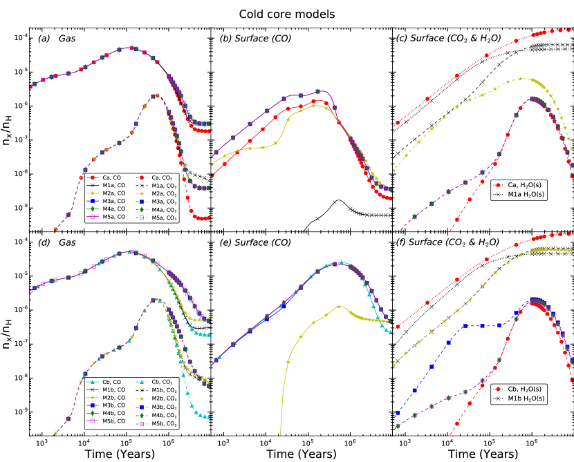
Figure 1: Time variation of the abundance of CO (solid lines) and CO₂ (dashed lines) for cold-core models are shown. Surface water abundance for Ca/Cb and M1a/M1b models are shown for reference using dotted lines. Panel (a) shows gas-phase abundances of CO and CO₂, (b) and (c) show surface abundances of CO and CO₂ respectively. All the abundances are plotted with respect to the total hydrogen density. The top panel is for $\mathcal{R}_{i}$ = 0.3 and bottom panel for 0.5. Legends for CO and CO₂ are same for all the panels. For colour figures please see the online version.

6.1 CO and CO₂

Figure 1 shows the time variation of the gas-phase abundance of CO and CO₂ for all the six models that belong to the cold cores. The top and bottom panels show abundances for $\mathcal{R}_{i}$ = 0.3 and 0.5 respectively, for different $\mathcal{R}_{CO}$. The solid and dashed lines represent CO and CO₂ abundances, respectively. It is evident that gas-phase CO abundance profile (Figure 1a, d) for all the models is almost same till 5 $\times$ 10⁵ years, and peak abundance comes around at 5.2 $\times$ 10^-5 and at $\sim$ 10⁵ yrs. Deviation in CO abundances for different models is not large and stays within a factor of 2.5 between the maximum (model M5) and minimum value (model Ca for $\mathcal{R}_{i}$ = 0.3 and Cb for 0.5). The gas-phase abundance for CO₂ is also mostly similar for all the six models, and it only deviates at the late times like CO. The pattern of deviation is also similar to that of CO, i.e., the model M5 has the maximum abundance and model Ca/Cb the least. The difference in abundance between these two models is nearly one order of magnitude. Interestingly, for the most of time evolution, the abundance of CO and CO₂ for model M1 for which CO diffusion is fastest is closer to the model abundance of M5, for which diffusion rate of CO is slowest. Thus gas-phase CO and CO₂ abundances got affected only at late times. It is expected since CO is efficiently formed in the gas-phase, the only way by which a difference could occur is via desorption processes. In cold cores, thermal desorption is ineffective, and the effect of non-thermal desorption is seen at late times. Therefore, deviations in gas-phase abundances are seen at late times.

In the Figure 1b and Figure 1e, CO abundances for models with $\mathcal{R}_{i}$ ($E_{\textrm{b, i}}$/$E_{\textrm{d, i}}$) = 0.3 and 0.5 are plotted respectively for varying $\mathcal{R}_{CO}$ ($E_{\textrm{b, CO}}$/$E_{\textrm{d, CO}}$). The abundance of surface H₂O for Ca/Cb and M1a/M1b models is also shown in the Figure 1c/f using the dotted lines for reference. In the top panel (Figure 1b) with $\mathcal{R}_{i}$ = 0.3, the profiles for $\mathcal{R}_{CO}$ = 0.3 (M3), 0.4 (M4), and 0.5 (M5) have almost no difference with a peak value of, 2.8 $\times$ 10^-6 (5 % of water), which is followed by Ca (1.5 $\times$ 10^-6, 3 % of water), M2a (1 $\times$ 10^-6, 2 % of water), M1a (1.7 $\times$ 10^-9, $<$ 0.01 % of water). In the bottom panel ($\mathcal{R}_{i}$ = 0.5), models Cb, M3b, M4b, and M5b have almost no difference and having a peak abundance between 2.3 - 2.6 $\times$ 10^-5 (27 - 30 % when compared with water). Model M2b ($\mathcal{R}_{CO}$ = 0.2) have a peak abundance of 1.3 $\times$ 10^-6 (3 % of water), whereas M1a ($\mathcal{R}_{CO}$ = 0.1) model has a very low abundance of solid CO. Thus it is clear the solid CO abundances increases when its mobility decreases but once the $\mathcal{R}_{CO}\geq 0.3$, the change in abundance is small. The solid CO abundance is very low for models M1a, b and M2a, b due to the fast recombination of CO to form other species. Also except for Model M1, solid CO abundance is greater for $\mathcal{R}_{i}$ = 0.5 (bottom panel) when compared between $\mathcal{R}_{i}$ = 0.3 (top panel), due to the slower conversion of CO into the other species.

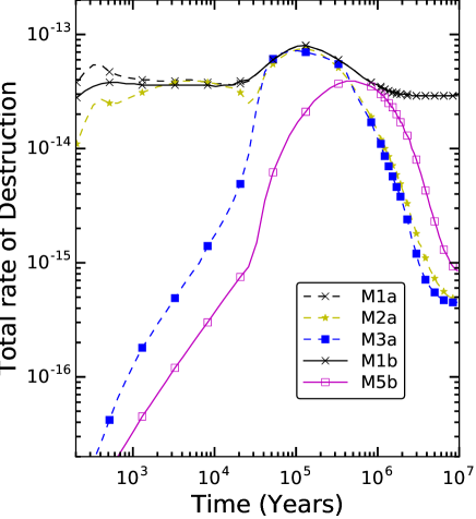
Figure 2: Time variation of the total rate of destruction (cm^-3s^-1) of solid CO is shown for assorted cold-core models. For colour figures please see the online version.

To investigate farther, in Figure 2, the total destruction rate (r${}_{\textrm{CO, pd}}$) which is obtained by adding all the individual rates in which CO is a reaction partner is plotted as a function of time for the assorted models. It is evident that the r${}_{\textrm{CO, pd}}$ for model M1 ($\mathcal{R}_{CO}$ = 0.1) and M2 ($\mathcal{R}_{CO}$ = 0.2) is always higher compared to other models, especially at smaller $t$, when it is significantly higher than the other models. For other models r${}_{\textrm{CO, pd}}$, gradually increases with time. The solid CO is primarily destroyed by the following two reactions:

$$CO+H\rightarrow HCO,$$ (16)

and

$$CO+OH\rightarrow CO_{2}+H.$$ (17)

For both ($E_{\textrm{b, i}}$/$E_{\textrm{d, i}}$ = 0.3 and 0.5) versions of C, M3, M4, and M5 the solid CO is primarily destroyed by Eq. 16, i.e., via hydrogenation. Whereas, for Model M1 and M2, the most dominant destruction pathway is always Eq. 17. Thus when CO mobility is large ($\mathcal{R}_{CO}\leq 0.2$), formation of CO₂ is preferred, otherwise it is hydrogenated to form HCO.

The peak total destruction rate for both the versions of C, M1, M2, M3, M4 is $\sim$ 8 $\times$ 10^-14 cm^-3s^-1 and comes between 10⁵ and 2 $\times$ 10⁵ yrs. For models, Cb and M5b, the peak r${}_{\textrm{CO, pd}}$ is lower by a factor of two and comes at a later time (around 4 $\times$ 10⁵ yrs). It implies that due to higher diffusion barrier, CO is destroyed relatively slowly. Thus solid CO abundance is higher for these models.

Time variation of abundance of solid CO₂ is shown for all the models in the Figure 1c and f for cold cores. Except for models M1a and M2a, for all the other models, the peak solid CO₂ abundance varies between (2 - 2.2) $\times$ 10^-6 (between 1 - 2 % of water). For model M1a ($\mathcal{R}_{CO}$ = 0.1 and $\mathcal{R}_{i}$ = 0.3), CO₂ is produced very efficiently as shown in Figure 1c. Peak solid CO₂ reaches close to the water ice abundance, which is the most abundant ice on the dust grains. Also, from Figure 1c, it is clear that for the model M1 water abundance is lower by at least a factor of two when compared to other models. Since both CO₂ and water formation requires OH radicals, an efficient CO₂ formation due to faster CO diffusion rate, reduces OH radicals available for water formation, thereby decreasing its abundance. Besides for models M1a and M2a the abundance of CO₂ starts to build-up earlier in time and remains flat. In the bottom panel, abundance for $\mathcal{R}_{i}$ = 0.5 is shown. The abundances are similar to as $\mathcal{R}_{i}$ = 0.3, except for M2b model ($\mathcal{R}_{CO}$ = 0.2), for which the solid CO₂ abundance is higher compared to the M1b.

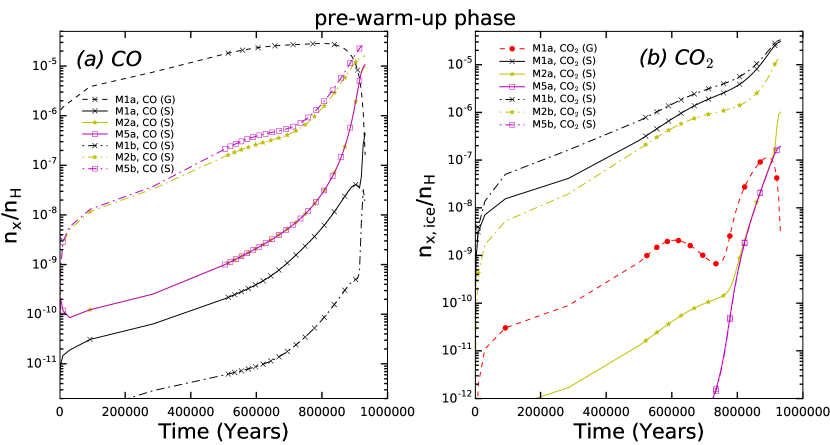
Figure 3: Time variation of CO (a) and CO₂ (b) for assorted models are shown for the pre-warm-up phase. Gas phase models with dashed lines are shown for M1 model only, since the abundance is similar. For colour figures please see the online version.

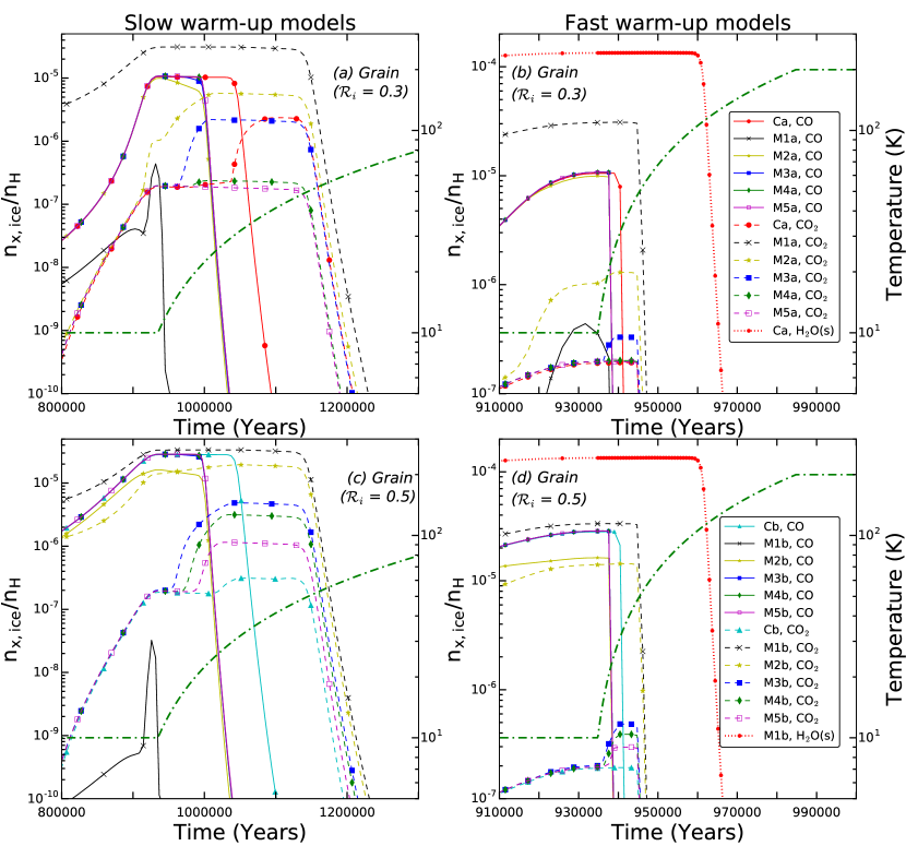
Figure 4: Time variation of the abundance of CO (solid lines), CO₂ (dashed lines), are shown for all the warm-up models for $\mathcal{R}_{i}$ = 0.3 and 0.5 in top and bottom panel respectively. The surface water (dotted line) for Ca model is shown for reference (other models have similar abundances). Panels (a) and (c) are for low mass star formation (slow heating), whereas (b) and (d) are for high mass star formation (fast heating). Legends for CO and CO₂ applies for all the panels. Gas/grain temperature as a function of time is shown using dot-dashed (green) line and scale is provided in the opposite y-axis. For colour figures please see the online version.

Abundance profiles of CO and CO₂ for warm-up models are shown in the Figure 3 and 4. As described in the §5, that the warm-up models have two phases. The abundance profile of the first phase in which density and visual extinction are changing at constant temperature (10 K) is shown in the Figure 3. In the pre warm-up phase, the surface CO abundance increases with decreasing diffusion rate, whereas for CO₂ show the opposite trend, that is the model M1 which have fastest diffusion have the highest abundance. Also difference in gas-phase abundances of CO and CO₂ between various models during the pre-warm-up phase is small.

Figure 4 shows the abundances of solid CO for the warm-up and the post-warm-up phases for $\mathcal{R}_{i}=0.3$ and $0.5$ in the top and bottom panel, respectively. For both $\mathcal{R}_{i}=$ 0.3 and 0.5, models with $\mathcal{R}_{CO}$ = 0.1 (M1a and M1b) have the lowest abundance ($\sim$ 0.4 % of water). Thus faster diffusion of solid CO resulted in the formation of CO₂. For other models, solid CO abundance is always large for $\mathcal{R}_{i}=$ 0.5 with a peak value of $\sim$ 3 $\times$ 10^-5 ($\sim$ 22 % of water) when compared with $\mathcal{R}_{i}=$ 0.3, which show a peak abundance of $\sim$ 1 $\times$ 10^-5 ($\sim$ 8 % of water). The model abundances are similar for both the fast and slow warm-up models. The models (Ca and Cb) for which coverage dependent barrier energies are used, CO desorbed at relatively higher temperatures when compared to the other models since its barrier for desorption increases with decreasing coverage. Since by $\sim$ 20 K, almost the entire CO is back to the gas phase due to the onset of thermal desorption due to warm-up, involvement of solid CO in the grain surface chemistry above this temperature will be limited.

The surface CO₂ abundances for the slow warm-up models are shown in the Figure 4a ($\mathcal{R}_{i}=0.3$), and c ($\mathcal{R}_{CO}=0.5$). In both cases solid CO₂ abundances increase as $\mathcal{R}_{CO}$ is decreased. The peak solid CO₂ abundance for both $\mathcal{R}_{i}=0.3$ and $0.5$ comes for M1a and M1b model, which is around $\sim$ 3 $\times$ 10^-5 ($\sim$ 30 %). There is a notable difference between M2a and M2b between $\mathcal{R}_{i}=0.3$ and $0.5$, for the later case solid CO₂ is higher by a factor of four. It can be due to the slower diffusion of other species which resulted lesser consumption of solid CO. For faster warm-up similar behaviour for M1 and M2 model is observed, but for other models there is almost no difference in the solid CO₂ abundance profile.

For both CO and CO₂, the surface abundance is similar for models with $\mathcal{R}_{CO}$ ($E_{\textrm{b, CO}}$/$E_{\textrm{d, CO}})>$ 0.2 for all the three physical conditions. Thus above a certain critical diffusion barrier, abundances of CO of CO₂ species remain unchanged due to lack of CO mobility.

A large difference in the solid CO₂ abundance in the M1 model (CO diffusion is the fastest) between warm-up and dense cloud models are seen. In the dense cloud, CO₂ abundance ($\sim$ 140% of water) for M1 model becomes greater than water abundance but only a moderate increase ($\sim$ 30% of water) is observed in the corresponding warm-up models. It is clear from Figure 3a gaseous CO in the warm-up models increases rapidly at late times. Therefore, CO accreted to the grain surface towards the end of the free fall collapse phase (density rises much faster towards the end). However by that time a significant amount of O/OH required to form CO₂ ice is used up to form other species especially water; which resulted in the lower abundance of solid CO₂ for the M1 model in warm-up models. On the other hand, in the dense cloud, the density and visual extinction are always relatively higher at the early phase, which resulted in depletion of more CO on the grain relatively earlier than warm-up models. Thus physical conditions played a role to negate the effect of faster diffusion in the warm-up models.

6.2 HCO, H₂CO, CH₃OH, and OCS

Figure 5 show the time variation of the abundance of HCO, H₂CO, CH₃OH, and OCS for the assorted cold core models. The solid and dashed lines represent the gas-phase and grain surface abundances respectively. The results demonstrate that surface abundance of HCO and OCS are always low, whereas surface abundance is high for H₂CO and CH₃OH. Also, models with $\mathcal{R}_{CO}$ ($E_{\textrm{b, CO}}$/$E_{\textrm{d, CO}})>0.2$, have almost similar surface abundances for all the species.

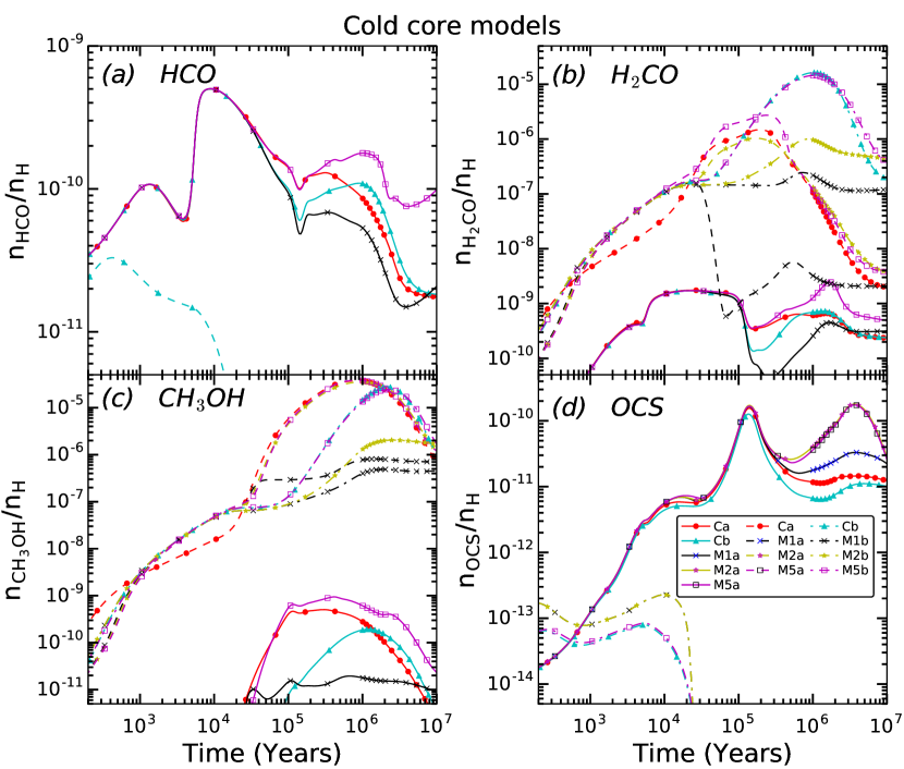
Figure 5: Time variation of gas (solid lines) and surface (dashed lines) abundance of HCO, H₂CO, CH₃OH, and OCS for the assorted cold core models are shown. Model abundances of M3 and M4 are similar to model M5, therefore not shown. For colour figures please see the online version.

For cold core models, the peak gas-phase abundance of HCO is almost same for all the models although abundance profile starts to diverge for time $>$ 4 $\times$ 10⁴ years. The divergence is mainly due to various types of non-thermal desorption such as reactive desorption, due to which $\sim$ 1 % is desorbed into the gas-phase. On the surface, HCO is efficiently produced, but abundance is low for all the models due to very efficient hydrogenation to form H₂CO, which have a large abundance. When HCO is produced, a small fraction is also ejected to the gas-phase, which can cause a difference in the gas-phase HCO abundance, provided its destruction rate in the gas-phase is slower than the rate of reactive desorption. Besides, Formation and destruction of HCO, H₂CO, and CH₃OH are closely linked, for an example the most dominant gas-phase formation route at late times for HCO is due to the reaction between H₂COH⁺ and electron. The production of H₂COH⁺ in the gas-phase occurs via the reaction between H₂CO/CH₃OH with various ions, e.g., H₃⁺. Thus reactive desorption of H₂CO/CH₃OH will also play a role in the abundance variation of gas-phase HCO. The solid HCO has a somewhat higher abundance for models Cb and M5b with $\mathcal{R}_{i}$ = 0.5.

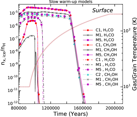
Figure 6: Time variation of surface abundance of H₂CO and CH₃OH, for assorted models with slow warm-up are shown. Gas/grain temperature as a function of time is shown using dotted line (red) and scale is provided in the opposite y-axis. Legends apply to both the plots.

Figure 5b show the abundance variation of H₂CO for assorted cold core models. Although gas-phase abundance is similar for all the models except, with a moderate variation ($\sim$ factor of three) in abundance between different models after 10⁵ yrs, the surface H₂CO varies significantly from one model to the other. Highest peak abundance for surface H₂CO is 1.6 $\times$ 10^-5 (15.6 % of water) for Cb, followed by the M5b model for which abundance is 1.5 $\times$ 10^-5 (14 % of water). For other models, peak surface abundance is reduced by at least a factor of six and model M1a having the lowest abundance. It is to be noted that despite the high surface abundance, gas-phase abundance of H₂CO is low, due to the absence of efficient desorption mechanisms at 10 K.

Figure 5c shows the abundance variation of CH₃OH for assorted dense cloud models. It is primarily formed on the surface of the dust grains. Abundance profile of CH₃OH also exhibits that for $\mathcal{R}_{CO}>0.2$, variation in abundance from one model to the other is small, which is true for both $\mathcal{R}_{i}=$ 0.3 and 0.5. Models with $\mathcal{R}_{i}=$ 0.3 have higher surface abundance compared to the corresponding models with $\mathcal{R}_{i}=$ 0.5. Maximum solid CH₃OH is formed for $\mathcal{R}_{i}=$ 0.3 and $\mathcal{R}_{CO}\geq 0.2$, which is $\sim$ 3.5 $\times$ 10^-5 ($\sim$ 38 % of water). For models with $\mathcal{R}_{i}=$ 0.5 and $\mathcal{R}_{CO}>0.2$ peak abundance is 2.5 $\times$ 10^-5 (20 % of water). The lowest abundance of surface CH₃OH comes for the M1b model. Also, peak abundances for models with $\mathcal{R}_{i}=$ 0.5 comes at later times when compared with models for $\mathcal{R}_{i}=$ 0.3. It can be seen that for H₂CO, peak abundance comes for $\mathcal{R}_{i}=$ 0.5 models, whereas for CH₃OH, it comes for the $\mathcal{R}_{i}=$ 0.3. It is due to the slow conversion of H₂CO to CH₃OH due to slower diffusion. Whereas, for CH₃OH, models with $\mathcal{R}_{i}=$ 0.3 had a higher abundance due to faster diffusion, which results in quick conversion of H₂CO to CH₃OH via hydrogenation. For both the species, model M1 for which CO diffusion is the fastest, the abundance is the lowest since CO quickly converted to CO₂ instead of getting hydrogenated.

Finally, Figure 5d shows the abundance variation of OCS for assorted cold core models; all the models have nearly the same peak gas-phase abundance and similar profiles till about 10⁵ years. The abundance varies only at the later times. The gas-phase abundance of OCS is low $\sim$ 10^-10 to 10^-11; therefore, a small change in the abundance of more abundant reactants which are involve in its formation can account for the late time variation. The OCS in the gas-phase is mostly produced either from HOCS⁺ or SO, which reacts with ions like HCO⁺, CH₃⁺, H₃⁺, etc. to produce OCS. Besides, a major complication comes because OCS can also be converted to HOCS⁺, so their production is interlinked. Solid OCS abundance is low for all the cold core models.

Selected slow heating warm-up model abundances for solid H₂CO and CH₃OH are shown in Figure 6; abundance does not vary from one model to the other except model for M1, for which abundance is lower by a factor of 10. The time variation of abundance of CH₃OH also show similar trends. Abundance of HCO and OCS are small $<10^{-10}$ therefore not shown.

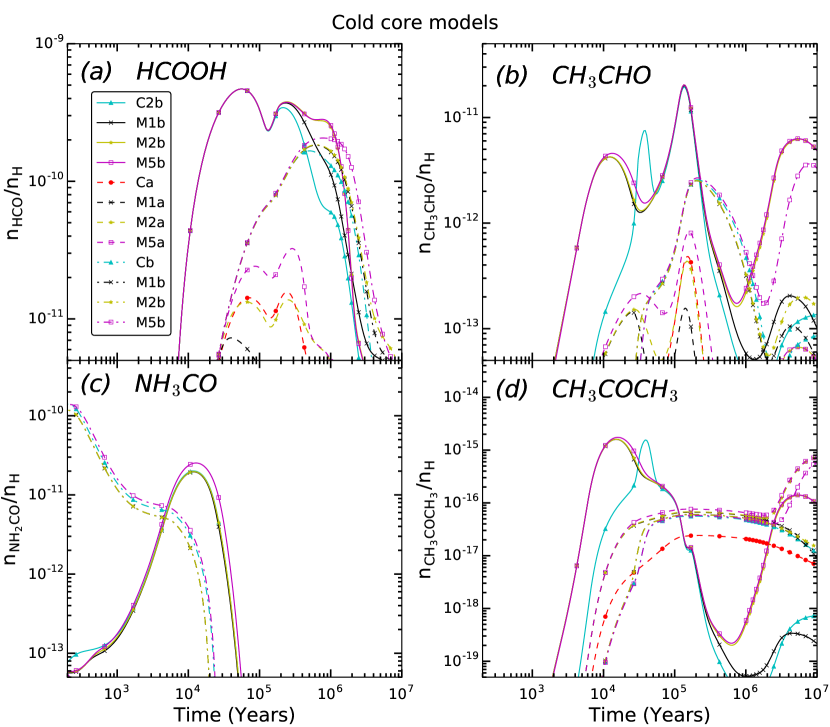
Figure 7: Time variation of gas (solid lines) and surface (dashed lines for $\mathcal{R}_{i}=0.3$, and dot-dashed lines for $\mathcal{R}_{i}=0.5$) abundance of HCOOH, CH₃CHO, NH₃CO, and CH₃COCH₃ for assorted cold core models are shown. Legends apply to all. For colour figures please see the online version.

6.3 HCOOH, CH₃CHO, NH₃CO, and CH₃COCH₃

Time variation of gas (solid lines) and surface (dashed lines for $\mathcal{R}_{i}=0.3$, and dot-dashed lines for $\mathcal{R}_{i}=0.5$) abundance of HCOOH, CH₃CHO, NH₃CO, and CH₃COCH₃ for the assorted dense cloud models are shown in the Figure 7. Since surface abundances of these species are low, warm-up model results are not discussed although peak abundances are shown in Table 5. Only species in the bunch which could have a noticeable amount of surface abundance is HCOOH. Its, gas-phase abundance is similar for all the models except the usual deviation at late times, while the surface abundance of HCOOH is lower and varies from one model to the other after 10⁴ yrs. The models for which $\mathcal{R}_{i}=0.5$, have nearly one order of magnitude higher abundance compared to the models having $\mathcal{R}_{i}=0.3$. Also, for both the cases abundances are nearly same for $\mathcal{R}_{CO}>0.2$. Compared to the dense cloud and fast warm-up models, HCOOH abundance increases for slow warm-up models. For acetaldehyde (CH₃CHO), the gas-phase abundance for all the models is similar till about 10⁶ yrs and having similar peak abundances, except for Cb model. Its surface abundance varies significantly from one model to the other, although the abundance is low; therefore, it will be difficult to detect. Both the formamide (NH₃CO) and acetone (CH₃COCH₃) have low gas-phase and surface abundance for all the models. Thus although there are variations in abundances for HCOOH, CH₃CHO, NH₃CO, and CH₃COCH₃ from one model to the other; none of the models increase the production significantly so that their abundance is above the present day detection limit on the ice. The capability of detection of ice is expected to increase significantly due to JWST mission, which can conclusively detect molecules like HCOOH. Also, formation mechanism of these complex molecules need to be revisited since at present they are not efficient enough.

Figure 8: Time variation of abundance of assorted species when activation energy for H + CO reaction is reduced to 1500 K (dashed lines) following Andersson et al. (2011) from 2500 K (solid lines) for the cold core models. For colour figures please see the online version.

6.4 Effect of Activation Energy

It is pertinent to discuss the effect of activation energy for the reactions for which multiple measurements are available. For the first step in Reaction 1, we have presented results having the activation energy of 2500 K. In an another measurement Andersson et al. (2011) found the activation energy to be as low as 1500 K. Figure 8 compares abundances between these two activation energies for cold core models. Models with activation energy of 1500 K shows higher HCO abundance for all the models for both $\mathcal{R}_{i}$ = 0.3 and 0.5. HCO can form H₂CO upon hydrogenation or CO₂ by reacting with atomic oxygen. Since hydrogen is much more mobile than oxygen, H₂CO is produced in higher quantity for all the models as can be seen in Figure 8b. For CO₂ the trend is reversed for models with $\mathcal{R}_{CO}$ = 0.1 and 0.2, for other models deviation is small. For CO₂ formation via 3, different activation energies (298 and 1580 K) did not yield any significant difference since it is not the most dominant formation pathways for CO₂ formation for any model.

6.5 Effect of pre-exponential factor

The diffusion rate is also depends on pre-exponential factor ($\nu_{0}$) as evident from the Equation 10, therefore, it is pertinent to discuss its effect. The solid CO measurements of Karssemeijer et al. (2014) and Lauck et al. (2015) reported D₀ values of 9.2 $\times$ 10^-10 and 3.1 $\times$ 10^-12 cm² s^-1 respectively. The value of $\nu_{0}$ can be roughly estimated by assuming, $\nu_{0}=D_{0}/a^{2}$, where, $a\sim 3\times 10^{-8}$cm is the typical hopping distance, which comes out to be $\sim$ 10⁶ and $\sim$ 3 $\times$ 10³ s^-1 for Karssemeijer et al. (2014) and Lauck et al. (2015) respectively. Also, He et al. (2018) found this value in the range of 10⁸ - 10⁹ s^-1. Where as Kouchi et al. (2020), considered pre-exponential factor using Equation 11 for their model. To test the dependence on $\nu_{0}$, four additional models are run with E_b from Lauck et al. (2015), Karssemeijer et al. (2014), He et al. (2018), and Kouchi et al. (2020) with $\nu_{0}$ of 3 $\times$ 10³, $\sim$ 10⁶,10⁸, and 10¹² s^-1 respectively. The time variation of abundance of CO and CO₂ for these models along with the M1a model are shown in the Figure 9. It can clearly be found that there is almost no difference between these models. Abundances for these models are similar to M3a model abundance and significantly different than model M1a. Outcome is in line with other models, i.e., for $\mathcal{R}_{CO}>0.2$, i.e, for slower diffusion rates of CO no appreciable difference in abundance is found for both CO and CO₂.

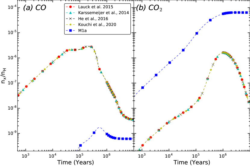
Figure 9: Time variation of solid abundance of CO and CO₂ with various combination of E_b and $\nu_{0}$ and model M1a. Legends applies to both the panel.

7 Comparison with Observations

Figure 10 shows the comparison with the observed range for CO, CO₂, CH₃OH, and H₂CO; and Table 5 shows observed and peak model abundances in water percentage (first row) as well as relative to the total hydrogen (second row) for selected surface species for all the three different physical conditions. We recall the model descriptions once more. Models were run by varying $\mathcal{R}_{CO}$ ($E_{\textrm{b, CO}}$/$E_{\textrm{d, CO}}$) between 0.1 and 0.5 and designated as M1, M2, M3, M4, and M5, and one model is run with coverage-dependent binding energy for CO designated using ‘C’. Each such model is further classified using the alphabet ‘a’ and ‘b’ with $E_{\textrm{b, i}}$/$E_{\textrm{d, i}}$ = 0.3 and 0.5 respectively. Abundances are similar for M3, M4, and M5 models; therefore these models are represented by the M5 model, For dense cloud models (Figure 10a), CO abundances are in the observed range for Cb and M5b models for a considerably large span of time. For models Ca and M5a abundances are close to the lower limit of the observed values. Whereas, abundance for the M1 model is significantly lower than the observed abundances. For low (Figure 10e) and high mass (Figure 10i) star formation, model abundances fall within the observed range for all the models except model M1a, and M1b. It indicates that models for which CO diffusion is relatively slower can explain observed CO abundances better compared to the models with faster diffusion.

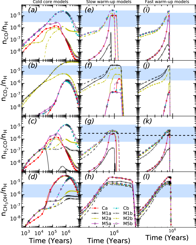
Figure 10: Comparison of observed abundances of CO, CO₂, H₂CO, and CH₃OH are shown for cold cloud (a, b, c ,and d), slow (e, f, g, and h) and fast (i, j, k, and l) heating warm-up models. Shaded regions represent the observed range for solid CO, CO₂, and CH₃OH. Whereas for H₂CO, the observed value is represented by the horizontal dashed line and shaded region represent a factor of six upper and lower abundance compared to the observed value. Each panel show Ca (circle), Cb (triangle), M3 (square), M5 (empty square), and M1 (x) models for a given species.

Table 5: Comparison between observed ice abundances and peak model abundances.

Species	Source	Observed∗	Models
			Ca	Cb	M1a - M2a	M2a - M2b	M5a - M5b
	Dense	9 - 67	3	30	4(-5) - 5(-7)	3.5 - 2.8	11 - 30
	clouds (DC)	3 - 21	1.5	25.6	1.7(-3) - 2(-5)	1 - 1.3	2.8 - 2.5
CO	Low-mass	$<$ 3 - 85	8	21	0.4 - 0.3	7.5 - 14	8 - 22
	Protostar (LMP)	$<$ 1.2 - 26	10.5	28.3	0.4 - 0.03	10 - 16.2	10.8 - 28.7
	Massive	3 - 26	8	21	0.4 - 0.03	7.5 - 14	8.1 - 22
	Protostar (MP)	$<$ 0.4 - 12.8	10.5	28.2	0.4 - 0.03	10 - 16.3	11 - 28.6
	Dense	14 - 43	1.4	1.5	136 - 144	10 - 12	1.4 - 2
	clouds	5.2 - 26	1.6	1.6	63.8 - 64.8	6.4 - 6	1.6 - 2
CO2	Low-mass	12 - 50	1.8	0.2	30.8 -35	4 - 17.4	1.7 - 3.8
	Protostar	2.4 - 25	2.4	0.31	31.2 - 33.6	5.8 - 19.5	2.2 - 5
	Massive	11 - 27	0.15	0.15	30.6 - 34.7	1 - 12.3	0.35 - 0.37
	Protostar	1.8 - 15.6	0.19	0.19	31 - 33.4	1.3 - 14.3	0.33 - 0.49
	Dense	5 - 12	37.5	21.8	1.8 - 1	36 - 4	39 - 19.5
	clouds	$<$ 0.6 - 6.6	37.5	27.8	0.8 - 0.5	35.2 - 2	38.5 - 24.5
CH3OH	Low-mass	1 - 30	22	9	13.3 - 7.7	23 - 8.8	23 - 9
	protostart	$<0.2$ - 15	28.4	9.6	13 - 7	29 - 9	29 - 9.7
	Massive	5 - 30	22.5	9	12.6 - 0.77	23 - 8.8	23 - 9
	Protostar	$<$ 0.4 - 16.6	28.4	9.6	12.5 - 7.1	29 - 9	29 - 10
	DC	-	3.8	16	2.3(-2) - 0.9	2.9 - 2	6.7 - 14
H2CO	LMP	$\sim$ 6	2	4.2	0.2 - 4.4	2.1 - 4	2.1 - 4.2
	MP	1 - 3	1.8	4.2	0.2 -4.4	1.9 - 4.1	1.9 - 4.2
	DC	$\sim$ 2	6(-5)	2(-4)	4(-5) - 4.3(-4)	6.9(-5) - 4(-4)	9.3(-5) - 2.4(-4)
HCOOH	LMP	1 - 9	0.08	0.14	0.5 - 0.23	0.2 - 0.17	0.13 - 0.1
	MP	3 - 7	1(-3)	1(-2)	3.8(-3) - 1.6(-2)	1(-3) - 2(-3)	1(-5) - 2(-3)
	DC	$<$ 2	2(-8)	9(-4)	7.6(-7) - 3.7(-2)	5(-7) - 3.7(-2)	3(-7)-3.8(-5)
OCS	LMP	-	9(-5)	1(-4)	6(-6) - 6(-5)	3(-6) - 4(-5)	2(-6) - 1(-5)
	MP	0.04 - 0.2	5(-5)	4(-4)	3(-5) - 1.5(-4)	3.6(-5) - 1.6(-4)	2.6(-5) - 1.4(-4)

* Observed abundances are from Boogert et al. (2015) and reference therein.
For a given source two sets of abundances are provided: the first row is in water % and second row is relative to n_H ($\times$ 10^-6)
Abundances relative to n_H is given only for CO, CO₂ and CH₃OH, since for other species abundances are low.

None of the model results can explain the solid CO₂ abundance in cold cores (Figure 10b), with an exception for the M1a, M1b, and M2b model for the certain time range. Ca, Cb, M3 - M5 models show significantly lower abundance, whereas, for model M1a and M1b, peak abundances are nearly three times larger compared to the upper bound of the observed abundance. Although over-produced, the faster diffusion of CO can increase the production of CO₂ ice significantly and can match observed abundances during the early phase of evolution. For slow and fast warm-up models (Figure 10f and j), both the versions of M1 and M2b models can match the observed abundance, whereas other models can not produce CO₂ in enough quantity to explain observed abundances. In this context it is important to note that to explain the observed abundance of solid CO₂, Garrod & Pauly (2011) incorporated hydrogenation of oxygen atom while situated on top of a surface CO molecule thus forming OH on the top of a CO surface. In this prescription, the only surface diffusion required to produce CO₂ is that of atomic hydrogen not CO or oxygen atom which are slower than atomic hydrogen when currently used diffusion barriers are considered. These authors successfully produced observed CO₂ abundances using their scheme. It implies that the CO diffusion rate should be similar to that of atomic hydrogen to explain observed CO₂ abundances. Besides, higher CO₂ abundance could also be found, if the initial dust temperature is relatively higher (15 - 20 K). It is found in the star-forming regions of Large and Small Magellanic clouds (Acharyya & Herbst (2015, 2016)), where, higher CO₂/H₂O is observed (dust temperatures are believed to be higher than the dust in our galaxy). Similar results were also found by Kouchi et al. (2020), using the model of Furuya et al. (2015). Similarly, Drozdovskaya et al. (2016) found higher solid CO₂ abundance in protoplanetary disks via grain surface reaction of OH with CO, due to enhanced photodissociation of H₂O. Thus the models with low diffusion barrier of solid CO does not improve the model abundance of solid CO and CO₂ towards the greater agreement with the observed abundances.

The surface abundance of HCO is always very low as can be seen from Figure 5a (cold cores models) and Figure 6 (slow warm-up models). It is yet to be observed, which is in line with the model results. The solid H₂CO is yet to be observed in cold clouds, all models over-produces (Figure 10c), particularly models with slower diffusion (Cb and M5b). It stays within the observed limit for warm-up models for both with the slow and fast heating (4th row in Table 5 and Figure 10g and k) except M1a. For CH₃OH, in dense clouds (Figure 10d), the M1a and M2b models are within the observed abundances. Apart from M1a, M1b and M2b models, all the other models tend to over-produce when compared with the observed abundances for most of the time ranges. For warm-up models (10h and l), abundances for Cb, M1b, M2b models are within observed limits (Table 5, 3rd row). The abundance of HCOOH for all the cold core models is significantly lower when compared with the observed abundances (Table 5, 5th row). The abundance increases for the slow warm-up model but still not sufficient to explain the observed abundances. Observed solid OCS abundance for cold cores have an upper limit of 2 $\%$ of water, whereas it is not observed in low-mass protostars. For massive protostars, its observed range is between 0.04 and 0.2 $\%$ of water (Table 5, 6th row). The model abundances are lower than the observed ranges for all the models.

8 Concluding Remarks

Impact of different diffusion barrier of CO in the grain surface chemistry is studied for three different physical conditions; dense clouds and two warm-up models with heating rates, which are representative of low and high mass star formation. For each of these conditions, six models were run; one coverage dependent binding energies and five models by varying $\mathcal{R}_{CO}$ (E${}_{\textrm{b, CO}}$/E${}_{\textrm{d, CO}}$) between 0.1 and 0.5. Besides for each value of $\mathcal{R}_{CO}$, two sets of models with $\mathcal{R}_{i}$ (E${}_{\textrm{b, i}}$/E${}_{\textrm{d, i}}$) = 0.3 and 0.5 are run. Major conclusions are as follows.

1. The abundance of CO increases with an increase in $\mathcal{R}_{CO}$, i.e., with decreasing diffusion rate. Abundance is higher for $\mathcal{R}_{i}$ = 0.5 compared to 0.3 except M1 models. Models with $\mathcal{R}_{CO}>$ 0.2, and Cb can explain the observed abundances, whereas other models, particularly, model M1a, b ($\mathcal{R}_{CO}$ = 0.1) provides significantly lower solid CO abundance when compared with the observed abundances due to efficient use of solid CO to form other species owing to its faster diffusion. For low and high mass star formation as well, model abundances fall within the observed range except for models with $\mathcal{R}_{CO}=0.1$.

2. For solid CO₂, none of the models can explain the observed abundances for the dense cloud. The models with faster diffusion over-produces CO₂ by a factor of three. Abundances are within the observed limit for the slow and fast warm-up models when $\mathcal{R}_{CO}\leq$ 0.2. Formation of CO₂ via CO + OH $\rightarrow$ CO₂ + H is favoured for $\mathcal{R}_{CO}\leq$ 0.2 otherwise, CO is hydrogenated to form HCO.

3. For H₂CO and CH₃OH agreement with observation can be found for almost all the models albeit in a limited range of parameter space. For H₂CO, peak abundance comes for $\mathcal{R}_{i}=$ 0.5 models, whereas for CH₃OH, it comes for the $\mathcal{R}_{i}=$ 0.3. For both the species, abundance is lowest for the models with the fastest CO-diffusion, since CO is efficiently converted to CO₂ instead of getting hydrogenated.

4. Formation of HCOOH, CH₃CHO, NH₃CO, and CH₃COCH₃ depends on the diffusion of CO. Their surface abundances differ significantly from one model to the other but, none of the models has any particular edge over others. None of the models produces these molecules in enough quantity so that their abundance is above the present-day detection limit on the ice. Among these four molecules, only solid HCOOH is likely to be observable, although models with slower diffusion produce more solid HCOOH compared to the models with faster diffusion but still not close to the observed abundance.

5. For $\mathcal{R}_{CO}>$ 0.2, the surface abundance of various species involving CO remain almost unchanged. Thus above a certain critical diffusion barrier, CO diffusion is slow and can not play a dominant role.

6. Finally, both $\mathcal{R}_{i}$ and $\mathcal{R}_{CO}$ plays a crucial role in the formation of molecules, and more laboratory measurements are required for both the parameters.

References

- Acharyya & Herbst (2015) Acharyya K., Herbst E., 2015, ApJ, 812, 142
- Acharyya & Herbst (2016) Acharyya K., Herbst E., 2016, ApJ, 822, 105
- Acharyya & Herbst (2017) Acharyya K., Herbst E., 2017, ApJ, 850, 105
- Acharyya et al. (2007) Acharyya K., Fuchs G. W., Fraser H. J., van Dishoeck E. F., Linnartz H., 2007, A&A, 466, 1005
- Acharyya et al. (2015) Acharyya K., Herbst E., Caravan R. L., Shannon R. J., Blitz M. A., Heard D. E., 2015, Molecular Physics, 113, 2243
- Allen & Robinson (1977) Allen M., Robinson G. W., 1977, ApJ, 212, 396
- Andersson et al. (2011) Andersson S., Goumans T. P. M., Arnaldsson A., 2011, Chemical Physics Letters, 513, 31
- Asgeirsson et al. (2017) Asgeirsson V. M., Jonssion H. M., Wikfeldt K. T. M., 2017, The Journal of Physical Chemistry C, 121, 1648
- Bisschop et al. (2006) Bisschop S. E., Fraser H. J., Öberg K. I., van Dishoeck E. F., Schlemmer S., 2006, A&A, 449, 1297
- Boogert et al. (2015) Boogert A. C. A., Gerakines P. A., Whittet D. C. B., 2015, ARA&A, 53, 541
- Brown et al. (1988) Brown P. D., Charnley S. B., Millar T. J., 1988, MNRAS, 231, 409
- Caselli et al. (1999) Caselli P., Walmsley C. M., Tafalla M., Dore L., Myers P. C., 1999, ApJ, 523, L165
- Collings et al. (2003) Collings M. P., Dever J. W., Fraser H. J., McCoustra M. R. S., 2003, Ap&SS, 285, 633
- Cooke et al. (2018) Cooke I. R., Öberg K. I., Fayolle E. C., Peeler Z., Bergner J. B., 2018, ApJ, 852, 75
- Drozdovskaya et al. (2016) Drozdovskaya M. N., Walsh C., van Dishoeck E. F., Furuya K., Marboeuf U., Thiabaud A., Harsono D., Visser R., 2016, MNRAS, 462, 977
- Fayolle et al. (2016) Fayolle E. C., Balfe J., Loomis R., Bergner J., Graninger D., Rajappan M., Öberg K. I., 2016, ApJ, 816, L28
- Fedoseev et al. (2015) Fedoseev G., Cuppen H. M., Ioppolo S., Lamberts T., Linnartz H., 2015, MNRAS, 448, 1288
- Fraser et al. (2002) Fraser H. J., Collings M. P., McCoustra M. R. S., 2002, Review of Scientific Instruments, 73, 2161
- Fuchs et al. (2009) Fuchs G. W., Cuppen H. M., Ioppolo S., Romanzin C., Bisschop S. E., Andersson S., van Dishoeck E. F., Linnartz H., 2009, A&A, 505, 629
- Furuya et al. (2015) Furuya K., Aikawa Y., Hincelin U., Hassel G. E., Bergin E. A., Vasyunin A. I., Herbst E., 2015, A&A, 584, A124
- Garrod (2013) Garrod R. T., 2013, ApJ, 765, 60
- Garrod & Pauly (2011) Garrod R. T., Pauly T., 2011, ApJ, 735, 15
- Garrod et al. (2007) Garrod R. T., Wakelam V., Herbst E., 2007, A&A, 467, 1103
- Garrod et al. (2008) Garrod R. T., Widicus Weaver S. L., Herbst E., 2008, ApJ, 682, 283
- Goumans et al. (2008) Goumans T. P. M., Uppal M. A., Brown W. A., 2008, MNRAS, 384, 1158
- Hama & Watanabe (2013) Hama T., Watanabe N., 2013, Chemical Reviews, 113, 8783
- Hama et al. (2012) Hama T., Kuwahata K., Watanabe N., Kouchi A., Kimura Y., Chigai T., Pirronello V., 2012, ApJ, 757, 185
- Harada et al. (2010) Harada N., Herbst E., Wakelam V., 2010, ApJ, 721, 1570
- Hasegawa et al. (1992) Hasegawa T. I., Herbst E., Leung C. M., 1992, ApJS, 82, 167
- He et al. (2016a) He J., Acharyya K., Vidali G., 2016a, ApJ, 823, 56
- He et al. (2016b) He J., Acharyya K., Vidali G., 2016b, ApJ, 825, 89
- He et al. (2018) He J., Emtiaz S., Vidali G., 2018, ApJ, 863, 156
- Herbst & Millar (2008) Herbst E., Millar T., 2008, The Chemistry of Cold Interstellar Cores. Imperial College Press, pp 1–54
- Herbst & van Dishoeck (2009) Herbst E., van Dishoeck E. F., 2009, ARA&A, 47, 427
- Karssemeijer et al. (2012) Karssemeijer L. J., Pedersen A., Jónsson H., Cuppen H. M., 2012, Physical Chemistry Chemical Physics (Incorporating Faraday Transactions), 14, 10844
- Karssemeijer et al. (2014) Karssemeijer L. J., Ioppolo S., van Hemert M. C., van der Avoird A., Allodi M. A., Blake G. A., Cuppen H. M., 2014, ApJ, 781, 16
- Katz et al. (1999) Katz N., Furman I., Biham O., Pirronello V., Vidali G., 1999, ApJ, 522, 305
- Kouchi et al. (2020) Kouchi A., Furuya K., Hama T., Chigai T., Kozasa T., Watanabe N., 2020, ApJ, 891, L22
- Lauck et al. (2015) Lauck T., Karssemeijer L., Shulenberger K., Rajappan M., Öberg K. I., Cuppen H. M., 2015, ApJ, 801, 118
- Livingston et al. (2002) Livingston F. E., Smith J. A., George S. M., 2002, Journal of Physical Chemistry A, 106, 6309
- Marchand et al. (2006) Marchand P., Riou S., Ayotte P., 2006, Journal of Physical Chemistry A, 110, 11654
- Minissale et al. (2013a) Minissale M., et al., 2013a, Phys. Rev. Lett., 111, 053201
- Minissale et al. (2013b) Minissale M., Congiu E., Manicò G., Pirronello V., Dulieu F., 2013b, A&A, 559, A49
- Minissale et al. (2014) Minissale M., Congiu E., Dulieu F., 2014, J. Chem. Phys., 140, 074705
- Mispelaer et al. (2013) Mispelaer F., et al., 2013, A&A, 555, A13
- Noble et al. (2012) Noble J. A., Congiu E., Dulieu F., Fraser H. J., 2012, MNRAS, 421, 768
- Öberg et al. (2009) Öberg K. I., Fayolle E. C., Cuppen H. M., van Dishoeck E. F., Linnartz H., 2009, A&A, 505, 183
- Roser et al. (2001) Roser J. E., Vidali G., Manicò G., Pirronello V., 2001, ApJ, 555, L61
- Ruaud et al. (2015) Ruaud M., Loison J. C., Hickson K. M., Gratier P., Hersant F., Wakelam V., 2015, MNRAS, 447, 4004
- Senevirathne et al. (2017) Senevirathne B., Andersson S., Dulieu F., Nyman G., 2017, Molecular Astrophysics, 6, 59
- Smith et al. (2016) Smith R. S., May R. A., Kay B. D., 2016, The Journal of Physical Chemistry B, 120, 1979
- Song & Kästner (2017) Song L., Kästner J., 2017, ApJ, 850, 118
- Tachikawa & Kawabata (2016) Tachikawa H., Kawabata H., 2016, Journal of Physical Chemistry A, 120, 6596
- Wakelam & Herbst (2008) Wakelam V., Herbst E., 2008, ApJ, 680, 371
- Wakelam et al. (2015) Wakelam V., et al., 2015, ApJS, 217, 20
- Watanabe et al. (2003) Watanabe N., Shiraki T., Kouchi A., 2003, ApJ, 588, L121
- Watanabe et al. (2004) Watanabe N., Nagaoka A., Shiraki T., Kouchi A., 2004, ApJ, 616, 638
- Watanabe et al. (2010) Watanabe N., Kimura Y., Kouchi A., Chigai T., Hama T., Pirronello V., 2010, ApJ, 714, L233
- Woon (1996) Woon D. E., 1996, J. Chem. Phys., 105, 9921
- Woon & Herbst (2009) Woon D. E., Herbst E., 2009, ApJS, 185, 273