Splitting of Fermi point of strongly interacting electrons in one dimension:
A nonlinear effect of spin-charge separation

Abstract

A system of one-dimensional electrons interacting via a short-range potential described by Hubbard model is considered in the regime of strong coupling using the Bethe ansatz approach. We study its momentum distribution function at zero temperature and find one additional singularity, at the $3k_{\mathrm{F}}$ point. We identify that the second singularity is of the same Luttinger liquid type as the low-energy one at $k_{\mathrm{F}}$. By calculating the spectral function simultaneously, we show that the second Luttinger liquid at $3k_{\mathrm{F}}$ is formed by charge modes only, unlike the known one around $k_{\mathrm{F}}$ consisting of both spin and charge modes. This result reveals the ability of the spin-charge separation effect to split the Fermi point of free electrons into two, demonstrating its robustness beyond the low-energy limit of Luttinger liquid where it was originally found.

Interactions have a dramatic effect on electrons in one dimension that has been attracting a significant interest in condensed-matter physics for a long time [1]. Their low-energy excitations become quantised density waves described by the Tomonaga-Luttinger liquid (TLL) theory based on linearisation of the spectrum around the Fermi points [2, 3, 4]. A hallmark prediction of this theory is separation of the spin and charge degrees of freedom of the underlying electrons into density waves of two distinct types with different velocities [5, 6]. Two linear dispersions originating from the Fermi point were observed in experiments on magnetotunnelling spectroscopy in semiconductors [7, 8], on photoemission in organic [9] and strongly anisotropic [10] crystals, and on time-resolved microscopy in cold atoms [11], establishing firmly this phenomenon.

Figure 1: (A) Momentum distribution function $n_{k}$ in the ground state of the model in Eq. (1) evaluated in the $U/t=\infty$ limit using Eqs. (6-9,11), where the two leading levels of the hierarchy of modes $l\leq 1$ were taken into account in the sum in Eq. (11), for $N=200$ particles (solid line) and for free particles $U/t=0$ (dashed line). Inset: Zoom-in around $3k_{\mathrm{F}}$. (B), (C), and (D) First derivative $dn_{k}/dk$ around the $k_{\mathrm{F}}$, $3k_{\mathrm{F}}$, and $5k_{\mathrm{F}}$ points respectively.

More recently, the theoretical interest was focused on spectral nonlinearity since it breaks construction of the TLL theory altogether [12] but, on the other hand, is unavoidable at any finite distance from the Fermi energy in a Fermi system. The Boltzmann equation approach to weakly interacting Fermi gas predicts a finite relaxation time due to nonlinearity [13, 14, 15], suggesting decay of the many-body modes. Application of the mobile impurity model to Luttinger liquids predicts survival of spin-charge separation at least in a weak sense, as a singularity–consisting of a mixture of spin and charge modes–at the spectral edge with nonlinear dispersion [16, 17, 18]. At the same time, the continuing experimental progress is starting to provide information on effects beyond the low-energy regime [19, 20, 21, 22, 23]. In one of these experiments [23], the spin-charge separated modes at low energy were observed to extend to the whole conduction band forming a pair of parabolic dispersions characterised by two incommensurate masses, raising the question if the spin-charge separation phenomenon manifests itself directly in other properties of the whole Fermi sea.

We explore such a possibility theoretically in this Letter by studying the momentum distribution function for a Fermi system with short-range interactions described by the Hubbard model, in which the spin-charge separation is well-established in the TLL limit [1]. Using the microscopic methods of Bethe ansatz in the strong coupling limit ($U=\infty$) not restricted to low energy [24], we find (at $T=0$) one extra divergence at $3k_{\mathrm{F}}$ in addition to the usual Fermi point at $k_{\mathrm{F}}$, see Fig. 1. Both singularities are of the same order, in the first derivative $dn_{k}/dk$, revealing the ability of spin-charge separation to split one Fermi point of free electrons into two [25]. It is a direct manifestation of this phenomenon in the whole Fermi sea, far away from the TLL limit. Around the second point, we find a power-law behaviour of $n_{k}$, $n_{k}\sim\dots+\mathrm{sgn}\left(k-3k_{\mathrm{F}}\right)\left|k-3k_{\mathrm{F}}\right|^{\alpha_{3k_{\mathrm{F}}}}$, with a real exponent of the TLL type $\alpha_{3k_{\mathrm{F}}}=0.787\pm 0.067$. However, this exponent does not correspond to the known exponents for spinful or spinless TLLs at $k_{\mathrm{F}}$ [1]. By calculating simultaneously the spectral function we show that, out of the spin-charge separated linear modes around $k_{\mathrm{F}}$, only the charge branch extends through the nonlinear region to form a TLL around $3k_{\mathrm{F}}$, identifying it as a TLL of a new kind.

We analyse fermions with spin-1/2 interacting via a short-range potential that are described by the 1D Hubbard model,

$$H=-t\sum_{j,\alpha}\left(c_{j\alpha}^{\dagger}c_{j+1,\alpha}+c_{j\alpha}^{\dagger}c_{j-1,\alpha}\right)+U\sum_{j}n_{j\uparrow}n_{j\downarrow},$$ (1)

where $c_{j\alpha}$ are the Fermi operators at site $j$, $\alpha$ is the spin-1/2 index $\uparrow$ or $\downarrow$, $n_{j\alpha}=c_{j\alpha}^{\dagger}c_{j\alpha}$ is the local density operator of the spin species $\alpha$, $t$ is the hoping amplitude describing the kinetic energy, and $U>0$ is the repulsive two-body interaction energy. Below, we consider the periodic boundary conditions, $c_{j+L}=c_{j}$, for a 1D lattice consisting of $L$ sites and for $N$-particle states we impose the constraint of low particle density, $N/L\ll 1$ [26]. In the strong-interaction limit, $U/t=\infty$, the spectrum of the model in Eq. (1) is given by the following Lieb-Wu equations [27, 28],

$$Lk_{j} -P_{s}=2\pi I_{j},$$ (2)

$$Nq_{m} -2\sum_{l\neq m}^{M}\varphi_{lm}=2\pi J_{m},$$ (3)

where $e^{i2\varphi_{lm}}=-\big{(}e^{iq_{l}+iq_{m}}+1-2e^{iq_{l}}\big{)}/\big{(}e^{iq_{l}+iq_{m}}+1-2e^{iq_{m}}\big{)}$ are the two-spinon scattering phases, the total spin momentum $P_{s}=\sum_{m}q_{m}$ is defined in the interval of $-\pi..\pi$, and $N$ non-equal integers $I_{j}$ and $M$ non-equal integers $J_{m}$ define the solution for the charge $k_{j}$ and spin $q_{m}$ (quasi)momenta of the $N$-particle state. This solution gives the eigenenergy of the many-body state as $E=t\sum_{j}k_{j}^{2}/2$ and its momentum as $P=\sum_{j}k_{j}$.

In the same limit, the eigenstates are factorised, $\left|\Psi\right\rangle=\left|\Psi_{c}\right\rangle\otimes\left|\Psi_{s}\right\rangle$, into a Slater determinant (like for free particles) for the charge and a Bethe wave function (like that for a Heisenberg chain) for the spin degrees of freedom [29, 28],

$$\left|\Psi_{c}\right\rangle =\frac{1}{L^{N}}\sum_{Q,\mathbf{j}}^{L}\left(-1\right)^{Q}e^{iQ\mathbf{k}\cdot\mathbf{j}}a_{j_{1}}^{\dagger}\cdots a_{j_{N}}^{\dagger}\left|0\right\rangle$$ (4)

$$\left|\Psi_{s}\right\rangle =\frac{1}{Z}\sum_{R,x_{1}<\dots<x_{M}}^{N}e^{i\sum_{l<m}\varphi_{R_{l}R_{m}}+iR\mathbf{q}\cdot\mathbf{x}}S_{x_{1}}^{+}\cdots S_{x_{M}}^{+}\left|\Downarrow\right\rangle$$ (5)

where $\mathbf{j}$ are charge coordinates of $N$ particles on the original Hubbard chain of length $L$, $\mathbf{x}$ are positions of say $M$ spins pointing up on the spin chain of $N$ spins forming the spin part of the wave function, and the sums over $Q$ and $R$ run over all possible permutations of $N$ momenta $k_{j}$ and $M$ momenta $q_{m}$ respectively. These wave functions are normalised to unity, with the non-trivial normalisation factor of the Bethe wave function being the determinant, $Z^{2}=\det\hat{Q}$, of an $M\times M$ matrix with the following diagonal $Q_{aa}=N-\sum_{l\neq a}^{M}4\left(1-\cos q_{l}\right)/\left(e^{iq_{l}}+e^{-iq_{a}}-2\right)/\left(e^{iq_{a}}+e^{-iq_{l}}-2\right)$ and off-diagonal $Q_{ab}=4\big{(}1-\cos q_{b}\big{)}/\big{(}e^{iq_{a}}+e^{-iq_{b}}-2\big{)}/\big{(}e^{iq_{b}}+e^{-iq_{a}}-2\big{)}$, with $a\neq b$, elements [30]. Here, the spinless Fermi $a_{j}^{\pm}$ and the purely spin $S_{j}^{\pm}$ operators can be recombined in the original electron operators $c_{j\alpha}^{\dagger}$ by introducing an insertion(deletion) of the spin-down state at a given position $x$ in the spin chain operator $I_{x}\left(D_{x}\right)$ as $c_{j\uparrow}^{\dagger}=a_{j}^{\dagger}S_{x}^{+}I_{x}$, $c_{j\downarrow}^{\dagger}=a_{j}^{\dagger}$ $I_{x}$, $c_{j\uparrow}=a_{j}D_{x}S_{x}^{-}$, and $c_{j\downarrow}=a_{j}D_{x}S_{x}^{-}S_{x}^{+}$ [31].

The zero temperature Green function is expressed in terms of the expectation values of the ladder operators as [32] $G_{\alpha}\left(k,E\right)=\sum_{f}\big{[}\big{|}\big{\langle}f\big{|}c_{k\alpha}^{\dagger}\big{|}0\big{\rangle}\big{|}^{2}/\big{(}E-E_{f}+i\eta\big{)}+\big{|}\big{\langle}f\big{|}c_{k\alpha}\big{|}0\big{\rangle}\big{|}^{2}/\big{(}E+E_{f}-i\eta\big{)}\big{]}$, where $c_{k\alpha}^{\pm}=\sum_{j}c_{j\alpha}^{\pm}e^{\pm ikj}/\sqrt{L}$ is the Fourier transform and $\eta$ is an infinitesimally small real number. The factorisation of the wave functions makes this calculation easier since the matrix elements becomes a product of two factors, $\left\langle f|c_{j\alpha}^{\pm}|0\right\rangle=\left\langle f|c_{j\alpha}^{\pm}|0\right\rangle_{c}\cdot\left\langle f|c_{j\alpha}^{\pm}|0\right\rangle_{s}$, where $0=\left(\mathbf{k}^{0},\mathbf{q}^{0}\right)$ and $f=\left(\mathbf{k}^{f},\mathbf{q}^{f}\right)$ the momenta of the ground and excited states. The model in Eq. (1) has the symmetry of swapping the spin indices $\uparrow\leftrightarrow\downarrow$, which its Green function also possesses, $G_{\uparrow}\left(k,E\right)=G_{\downarrow}\left(k,E\right)$. Therefore, we will consider only $\alpha=\uparrow$. The charge part of the matrix element is an expectation value with respect to the state in Eq. (4) that evaluates as an $N$-fold sum over coordinates $\mathbf{j}$ producing a determinant of the Vandermonde type. Then, application of the generalised Cauchy formula gives the following result for the annihilation operator $c_{j\uparrow}$ [33, *Penc97p, 35]

$$\big{<}f\big{|}c_{j\uparrow}\big{|}0\big{>}_{c}=\frac{2^{N-1}\sin^{N-1}\left(\frac{P_{s}^{f}-P_{s}^{0}}{2}\right)e^{i\left(P_{0}-P_{f}\right)j}}{L^{N-\frac{1}{2}}}\\ \times\frac{\prod_{i<j}^{N-1}\left(k_{i}^{f}-k_{j}^{f}\right)\prod_{i<j}^{N}\left(k_{i}^{0}-k_{j}^{0}\right)}{\prod_{i,j}^{N,N-1}\left(k_{j}^{f}-k_{i}^{0}\right)},$$ (6)

where $\big{<}f\big{|}c_{j\uparrow}\big{|}0\big{>}_{c}\equiv\big{<}\Psi_{c}^{f}\big{|}a_{j}\big{|}\Psi_{c}^{f}\big{>}$ and the low-density limit, in which $k_{j}^{0,f}\ll 1$, is already taken.

The spin part part of the matrix elements is an expectation value with respect to the states in Eq. (5) that is less straightforward to evaluate. A mathematical technique for dealing with these Bethe states analytically was invented in an algebraic form [36], leading to calculation of the correlation function for the non-iternarant quantum magnets described by the Heisenberg model [37, *Kitanine00, 39]. However, this result cannot be used here directly since the operators of the Hubbard model $c_{j\uparrow}^{\pm}$ change the length of the spin chain, making the constructions of [36] for the bra and ket states incompatible with each other. We resolve this problem by representing operators of one algebra (for the longer chain) through the other (for the shorter chain) and the spin operators of the extra site. Then, explicit evaluation of the expectation value in the spin subspace of the additional site restores applicability of the methods in [[Seethebookby][andreferencesthereinfordetails.]Korepin_book], and we obtain the spin part of the matrix element in terms of the determinant of an $M\times M$ matrix (see details of this calculation in [28]),

$$\big{<}f\big{|}c_{j\uparrow}\big{|}0\big{>}_{s}=\frac{\det\hat{R}}{Z_{0}Z_{f}}\prod_{i,j}^{M-1,M}\left(e^{iq_{i}^{f}}+e^{-iq_{j}^{0}}-2\right)\\ \times\prod_{i\neq j}^{M-1}\left(e^{iq_{i}^{f}}+e^{-iq_{j}^{f}}-2\right)^{-\frac{1}{2}}\prod_{i\neq j}^{M}\left(e^{iq_{i}^{0}}+e^{-iq_{j}^{0}}-2\right)^{-\frac{1}{2}},$$ (7)

where $\big{<}f\big{|}c_{j\uparrow}\big{|}0\big{>}_{s}\equiv\big{<}\Psi_{s}^{f}\big{|}D_{x}S^{-}\big{|}\Psi_{s}^{0}\big{>}$ and the elements of matrix $\hat{R}$ are

$$R_{ab} =\frac{e^{iq_{b}^{0}\left(N-1\right)}\prod_{j\neq a}^{M-1}\left(-\frac{e^{iq_{j}^{f}+iq_{b}^{0}}+1-2e^{iq_{j}^{f}}}{e^{iq_{j}^{f}+iq_{b}^{0}}+1-2e^{iq_{b}^{0}}}\right)-1}{\left(e^{-iq_{a}^{f}}-e^{-iq_{b}^{0}}\right)\left(e^{iq_{a}^{f}}+e^{-iq_{b}^{0}}-2\right)},$$ (8)

$$R_{Mb} =\frac{e^{ik_{b}^{0}}\prod_{i\neq b}^{M}\left(e^{iq_{i}^{0}}+e^{-iq_{b}^{0}}-2\right)}{\prod_{j}^{M-1}\left(e^{iq_{i}^{f}}+e^{-iq_{b}^{0}}-2\right)}$$ (9)

for $a<M$ and for $a=M$ respectively. Together Eqs. (6-9) give the complete analytical expression for the matrix element for the 1D Hubbard model. Repeating the same calculation for the matrix element of the creation operator, $\big{\langle}f\big{|}c_{k\uparrow}^{\dagger}\big{|}0\big{\rangle}$, we obtain the same expressions as in Eqs. (6-9), in which the momenta are swapped, $\mathbf{k}^{0},\mathbf{q}^{0}\leftrightarrow\mathbf{k}^{f},\mathbf{q}^{f}$, and the particle (spin) quantum number is increased by one, $N\rightarrow N+1$ ($M\rightarrow M+1$).

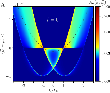
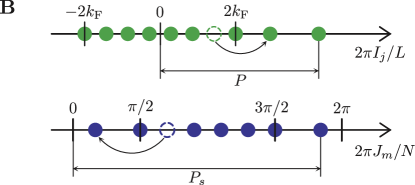
Figure 2: (A) Spectral function $A_{\alpha}\left(k,E\right)$ of the model in Eq. (1) evaluated in the $U/t=\infty$ limit using Eqs. (6-9,10) for $N=500$ particles, where only the leading level of the hierarchy $l=0$ was taken into account in the sum in Eq. (10). The single particle dispersion of free particles $U/t=0$ is superimposed as dashed line. (B) Two sets of integer numbers, $I_{j}$ for charge and $J_{m}$ for spin degrees of freedom, defining the Lieb-Wu equations (2,3) for an excited state with momentum $P$ and the total spin momentum $P_{s}$; two “electron-hole” pairs are shown as examples of lowering the level of the hierarchy, see text. For a spin-unpolarised system, the number of spin degrees of freedom is $M=N/2$ that makes the charges’ density twice larger than that of the spins.

The response of a many-body system to a single-particle excitation at a given momentum and energy is described by the spectral function, making this observable particularly interesting for the experiments on spectroscopy. It is related to Green function as $A_{\alpha}\left(k,E\right)=-\textrm{Im}G_{\alpha}\left(k,E\right)\textrm{sgn}\left(E-E_{0}\right)/\pi$ [32] giving

$$A_{\alpha}\left(k,E\right)=\sum_{f}\big{|}\big{<}f\big{|}c_{k\alpha}^{\dagger}\big{|}0\big{>}\big{|}^{2}\delta\left(E-E_{f}+E_{0}\right)\\ +\sum_{f}\big{|}\big{<}f\big{|}c_{k\alpha}\big{|}0\big{>}\big{|}^{2}\delta\left(E+E_{0}-E_{f}\right),$$ (10)

where the sum over the result in Eqs. (6-9) [40] needs to be evaluated over exponentially many final states $f$. It can be done based on emergence of the hierarchy of modes: Away from the low-energy regime around the Fermi points the many-body continuum splits itself into levels (consisting of a polynomial number of excitations on each of them) according to their spectral strength, which is proportional to integer powers of a small parameter $1/L^{2}$ [41, *OT16].

In the presence of spin and charge degrees of freedom this phenomenon manifests itself on the microscopic level in the following way. For the ground states, the charge and spin momenta form two Fermi seas that correspond to selecting the non-equal integer numbers in Eqs. (2,3) as $I_{j}=-N/2\dots N/2$ and $J_{m}=-\left(N-M\right)/2\dots\left(N+M\right)/2$ [27], see illustration in Fig. 2B. The charge part of the spectral amplitude for a generic excitation above this ground state, $\big{|}\big{<}f\big{|}c_{k\alpha}^{\dagger}\big{|}0\big{>}_{c}\big{|}^{2}$ given by Eq. (6), is vanishingly small in the thermodynamic limit since it is proportional to $1/L^{2N}$. However, the factor $k_{j}^{f}-k_{i}^{0}$ in the denominator of Eq. (6) produces a singularity that is cut off by $1/L$ cancelling a power of $1/L^{2}$ in the spectral amplitude each time a charge momentum of the excited state is equal to a momentum of the ground state. This property selects a specific set of the excitations, for which a charge is added above the ground–see the charge state in Fig. 2B–and for which the $1/L^{2N}$ factors is canceled altogether making $\big{|}\big{<}f\big{|}c_{k\alpha}^{\dagger}\big{|}0\big{>}_{c}\big{|}^{2}\sim 1$. Adding each “electron-hole” pairs of charges on top of these states multiplies the spectral amplitude by an extra small parameter $1/L^{2}$ since some powers of the normalisation factor $1/L^{2N}$ remain uncanceled.

For the spin part of the spectral amplitude, $\big{|}\big{<}f\big{|}c_{k\alpha}^{\dagger}\big{|}0\big{>}_{s}\big{|}^{2}$ given by Eq. (7), emergence of a small parameter is similar. The normalisation factor $1/\left(Z_{0}Z_{f}\right)$ makes the amplitude proportional to a vanishing in the thermodynamic limit factor $1/N^{2M}$ and the singularity $1/\big{(}e^{-iq_{a}^{f}}-e^{-iq_{b}^{0}}\big{)}$ in the matrix elements in Eq. (8) cancels it altogether for a subset of states, for which only one spin is added on top of the spin ground states–see the spin state in Fig. 2B–making $\big{|}\big{<}f\big{|}c_{k\alpha}^{\dagger}\big{|}0\big{>}_{s}\big{|}^{2}\sim 1$. Adding each “electron-hole” pair of spins on top multiplies the spectral amplitude by an extra small parameter $1/N^{2}$.

Combined, these two properties result in the hierarchy of modes for both types of the degrees of freedom, with the spectral power for the strongest excitations being of the order of $\big{|}\big{<}f\big{|}c_{k\alpha}^{\dagger}\big{|}0\big{>}\big{|}^{2}\sim 1$ and the subleading excitations being weak as $\big{|}\big{<}f\big{|}c_{k\alpha}^{\dagger}\big{|}0\big{>}\big{|}^{2}\sim 1/\big{(}N^{2m}L^{2n}\big{)}$, where $l=n+m>0$ and $n$ and $m$ are the numbers of extra “electron-hole” pairs in the charge and spin Fermi seas respectively. Close to the Fermi points this hierarchy of modes breaks down. The spectral amplitudes of all excitations become of the same order forming spin and charge density waves, and the spinful TLL theory becomes a better approach for calculating correlation functions [6, *Voit93].

Analysing first the nonlinear regime away from the Fermi points, we evaluate the spectral function in Eq. (10) numerically taking into account only the top level of the hierarchy $l=0$ in the sum over $f$ [43]. The result is presented in Fig. 2A, where the Fermi momentum is defined by the free particle limit as $k_{\mathrm{F}}=\pi N/2$ and the corresponding sum rule (which also includes the linear regime around the Fermi points) is already fulfilled as $2\int_{-\infty}^{\infty}dk\int_{-\infty}^{0}dEA\left(k,E\right)/N\simeq 61\%$ even for a large number of particles $N=500$. Unlike the case of spinless fermions [41, 42], the excitations at the top level of the hierarchy form a continuum for fermions with spin-1/2 since adding an electron with spin-1/2 adds simultaneously both charge and spin with two different momenta $P$ and $P_{s}$, see Fig. 2B. In this continuum, only two non-equivalent peaks emerge away from the Fermi points: One connects the $\pm k_{\mathrm{F}}$ points and the other connects the $-k_{\mathrm{F}},3k_{\mathrm{F}}$ points (or equivalently, the $-3k_{\mathrm{F}},k_{\mathrm{F}}$ points) on the $E=\mu$ line. Around the $\pm k_{\mathrm{F}}$ Fermi points, these nonlinear peaks become two linear peaks that are the manifestation of the collective spin (i.e spinon) and charge (i.e holon) modes predicted by the spinful TLL model at low energy [6, 5]. This identifies the nonlinear modes as being collective spin and charge excitations as well (see more details in [28]), and shows that the spin-charge separation still manifests itself in observables beyond the linear TLL limit.

The line shapes of the peaks away from the low-energy region have the form of divergent power-laws, e.g. the particular momentum-dependent exponent was predicted for the spinon mode (which correspond to the spectral edge at finite $U$) in [16, 44] and experimentally confirmed in [21]. The nonlinear holon and spinon modes were observed directly in the momentum-energy resolved magnetotunneling experiments in semiconductor quantum wires at intermediate coupling strength [20, 23] that strongly suggests their robustness also for interactions with finite range and of finite strength, beyond the regime of the present calculation.

The momentum distribution function is another observable of interest in the many-body systems. It can be obtained from Green function as $n_{k}=\int dE\allowbreak\Theta\left(E_{0}-E\right)\textrm{Im}G_{\alpha}\left(k,E\right)/\pi$ [32] giving

$$n_{k}=\sum_{f}\big{|}\big{<}f\big{|}c_{k\alpha}\big{|}0\big{>}\big{|}^{2}.$$ (11)

One of the regions of particular interest for this quantity is proximity of the Fermi point, in which the infinite number the “electron-hole” pairs has to be included in the sum over $f$. This can be, at least partially, accounted for by adding subleading levels of the hierarchy. The result of the numerical calculation for $N=200$ and $l\leq 1$ is presented in Fig. 1A, where the sum rule already accounts for $2\int dkn_{k}/N\simeq 86\%$ of the particles.

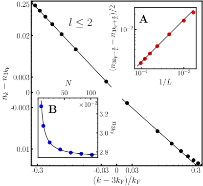
Figure 3: Momentum distribution function $n_{k}$ around $3k_{\mathrm{F}}$ on the log-log scale for $N=80$ particles, where the three leading levels of the hierarchy of modes $l\leq 2$ were taken into account in the sum in Eq. (11). The dashed solid lines are power-law functions for $k<3k_{\mathrm{F}}$ and for $k>3k_{\mathrm{F}}$ giving the exponent as $a_{3k_{\mathrm{F}}}=0.787\pm 0.067$, where the value is the average of the two and the error bars is the difference. Inset A: Finite size cutoff for $n_{k}$ as the function of inverse system size $1/L$ on the log-log scale at $3k_{\mathrm{F}}$. The solid line is a power-law fit giving $a_{3k_{\mathrm{F}}}=0.838$, within the accuracy of the fitting $n_{k}$ directly. Inset B: The value of $n_{k}$ at $3k_{\mathrm{F}}$ as a function of the particle number $N$. The solid line is a fit of finite size corrections, $n_{3k_{\mathrm{F}}}=C_{3k_{\mathrm{F}}}+b/N$, giving $C_{3k_{\mathrm{F}}}=0.027$.

Singularities in $n_{k}$ were introduced as the definition of a Fermi surface in many-body systems in the Luttinger theorem [45]. Here, we use this definition to interpret the result in Fig. 1. Due to the TLL physics, the singularity at $k_{\mathrm{F}}$ is weaker in 1D [46], e.g. instead of a discontinuity in $n_{k}$ in $D>1$ dimensions $n_{k}$ is finite, with a divergence appearing in $dn_{k}/dk$ in 1D, see Fig. 1B. Inspecting the result in Fig. 1A, we find a second singularity of same order at $3k_{\mathrm{F}}$, see Fig. 1C. And we find no divergencies at any other points, e.g. see Fig. 1D. The second singularity can be interpreted as a direct manifestation of spin-charge separation beyond the low-energy regime, which facilitates appearance of two Fermi points at different momenta since the density of nonlinear holons twice larger than that of the nonlinear spinons in a spin-unpolarised system. Note that $n_{k=0}\simeq 0.7$ in Fig. 1A is still smaller than $n_{k=0}=1$ for the free system so $\sim 30\%$ of particles is redistributed above $k_{\mathrm{F}}$ providing a significant amplitude around the $3k_{\mathrm{F}}$ point.

The coinciding order of both singularities suggests that the states around $3k_{\mathrm{F}}$ are also described by a TLL model, which predicts a power-law behaviour of the momentum distribution function [1],

$$n_{k}=C_{(3)k_{\mathrm{F}}}+\dots\mathrm{sgn}\left((3)k_{\mathrm{F}}-k\right)\left|k-(3)k_{\mathrm{F}}\right|^{\alpha_{(3)k_{\mathrm{F}}}},$$ (12)

where $\alpha_{(3)k_{\mathrm{F}}}$ is a real exponents and $C_{(3)k_{\mathrm{F}}}$ is the value of $n_{k}$ exactly at $\left(3\right)k_{\mathrm{F}}$. Fitting a linear function on a log-log plot of $n_{k}$ extracts the exponent around $3k_{\mathrm{F}}$ directly, see Fig. 3. Alternatively, the same exponent can be extracted from the finite size cutoff at $3k_{\mathrm{F}}$, see inset A in Fig. 3. Both methods give $a_{3k_{\mathrm{F}}}=0.787\pm 0.067$. The scaling of $n_{3k_{\mathrm{F}}}$ with the system size gives a finite amplitude in the thermodynamic limit, $C_{3k_{\mathrm{F}}}=0.027$, see inset B in Fig. 3. In all of these numerical calculations the number of the levels $l$ used in calculating Eq. (11) was increased until the next subleading level was giving only a small correction to the value of $n_{k}$ at each point. Application of the same procedure around $k_{\textrm{F}}$ gives $C_{k_{\mathrm{F}}}=0.477$ and $\alpha_{k_{\mathrm{F}}}=0.124\pm 0.020$ [28], which is the well-known result of the TLL theory $\alpha_{k_{\mathrm{F}}}=0.125$ [47, 48, 49]. However, only one attempt of using the TLL approach at $3k_{\mathrm{F}}$ was made in [50], in which $a_{3k_{\mathrm{F}}}=1.125$ was obtained, suggesting a lower order (in $d^{2}n_{k}/dk^{2}$) of the second singularity. This discrepancy can be attributed to using both spinon and holon modes in [50], while the present microscopic calculation shows in Fig. 2A that only the holon modes can form a TLL at $3k_{\mathrm{F}}$.

In conclusions, we have shown that spin-charge separation can split one Fermi surface into two. Together with the recent experimental observation of spin-charge splitting of the whole band in [23], it demonstrates that this phenomenon is more general than it was originally anticipated, and also that substantial features of the Fermi gas still survive in 1D despite formation of a genuine many-body continuum by the interactions.

I thank Andy Schofield for discussions and helpful comments. This work was funded by the Deutsche Forschungsgemeinschaft (DFG) via project number 461313466.

References

- Giamarchi [2003] T. Giamarchi, Quantum physics in one dimension (Clarendon press, Oxford, 2003).
- Tomonaga [1950] S. Tomonaga, Prog. Theor. Phys. 5, 544 (1950).
- Luttinger [1963] J. M. Luttinger, J. Math. Phys. 4, 1154 (1963).
- Haldane [1981] F. D. M. Haldane, J. Phys. C: Solid State Phys. 14, 2585 (1981).
- Voit [1993] J. Voit, Phys. Rev. B 47, 6740 (1993).
- Meden and Schönhammer [1992] V. Meden and K. Schönhammer, Phys. Rev. B 46, 15753 (1992).
- Auslaender et al. [2005] O. M. Auslaender, H. Steinberg, A. Yacoby, Y. Tserkovnyak, B. I. Halperin, K. W. Baldwin, L. N. Pfeiffer, and K. W. West, Science 308, 88 (2005).
- Jompol et al. [2009] Y. Jompol, C. J. B. Ford, J. P. Griffiths, I. Farrer, G. A. C. Jones, D. Anderson, D. A. Ritchie, T. W. Silk, and A. J. Schofield, Science 325, 597 (2009).
- Claessen et al. [2002] R. Claessen, M. Sing, U. Schwingenschlögl, P. Blaha, M. Dressel, and C. S. Jacobsen, Phys. Rev. Lett. 88, 096402 (2002).
- Kim et al. [2006] B. J. Kim, H. Koh, E. Rotenberg, S.-J. Oh, H. Eisaki, N. Motoyama, S. Uchida, T. Tohyama, S. Maekawa, Z.-X. Shen, and C. Kim, Nat. Phys. 2, 397 (2006).
- Vijayan et al. [2020] J. Vijayan, P. Sompet, G. Salomon, J. Koepsell, S. Hirthe, A. Bohrdt, F. Grusdt, I. Bloch, and C. Gross, Science 367, 186 (2020).
- Samokhin [1998] K. V. Samokhin, J. Phys. Condens. Matter 10, L533 (1998).
- Karzig et al. [2010] T. Karzig, L. I. Glazman, and F. von Oppen, Phys. Rev. Lett. 105, 226407 (2010).
- Levchenko and Micklitz [2021] A. Levchenko and T. Micklitz, J. Exp. Theor. Phys. 132, 675 (2021).
- Ristivojevic and Matveev [2021] Z. Ristivojevic and K. A. Matveev, Phys. Rev. Lett. 127, 086803 (2021).
- Imambekov and Glazman [2009] A. Imambekov and L. I. Glazman, Phys. Rev. Lett. 102, 126405 (2009).
- Schmidt et al. [2010] T. L. Schmidt, A. Imambekov, and L. I. Glazman, Phys. Rev. Lett. 104, 116403 (2010).
- Imambekov et al. [2012] A. Imambekov, T. L. Schmidt, and L. I. Glazman, Rev. Mod. Phys. 84, 1253 (2012).
- Barak et al. [2010] G. Barak, H. Steinberg, L. N. Pfeiffer, K. W. West, L. Glazman, F. von Oppen, and A. Yacoby, Nat. Phys. 6, 489 (2010).
- Moreno et al. [2016] M. Moreno, C. J. B. Ford, Y. Jin, J. P. Griffiths, I. Farrer, G. A. C. Jones, D. A. Ritchie, O. Tsyplyatyev, and A. J. Schofield, Nat. Commun. 7, 12784 (2016).
- Jin et al. [2019] Y. Jin, O. Tsyplyatyev, M. Moreno, A. Anthore, W. Tan, J. Griffiths, I. Farrer, D. Ritchie, L. Glazman, A. Schofield, and C. Ford, Nat. Commun. 10, 2821 (2019).
- Wang et al. [2020] S. Wang, S. Zhao, Z. Shi, F. Wu, Z. Zhao, L. Jiang, K. Watanabe, T. Taniguchi, A. Zettl, C. Zhou, and F. Wang, Nat. Mater. 19, 986 (2020).
- Vianez et al. [2021] P. M. T. Vianez, Y. Jin, M. Moreno, A. S. Anirban, A. Anthore, W. K. Tan, J. P. Griffiths, I. Farrer, D. A. Ritchie, A. J. Schofield, O. Tsyplyatyev, and C. J. B. Ford, arXiv:2102.05584 (2021).
- Korepin et al. [1993] V. E. Korepin, N. M. Bogoliubov, and A. G. Izergin, Quantum inverse scattering methods and correlation functions (Cambridge University Press, 1993).
- [25] The definition of a Fermi point (or surface) for a many-body system as a special point in was given by Luttinger and Haldane [45, 46].
- [26] This limit corresponds to the continuum model with a finite mass and a -functional density-density interaction, in which the mass is inversely proportional to the hopping amplitude , the interaction strength is proportional to , and the lattice parameter only plays the role of an ultraviolet cutoff.
- Lieb and Wu [1968] E. H. Lieb and F. Y. Wu, Phys. Rev. Lett. 20, 1445 (1968).
- [28] See Supplementary Material at https:// for details, which includes Refs. 51, 52, 53, 54, 55, 56, 57, 58.
- Ogata and Shiba [1990] M. Ogata and H. Shiba, Phys. Rev. B 41, 2326 (1990).
- Gaudin et al. [1981] M. Gaudin, B. M. McCoy, and T. T. Wu, Phys. Rev. D 23, 417 (1981).
- [31] While the and operators obey the regular Fermi and spin commutation rules, the insertion(deletion) operator () does not. In general, they also do not commute with the spin operators.
- Mahan [1990] G. D. Mahan, Many-particle physics (Plenum Press, 1990).
- Penc et al. [1996] K. Penc, K. Hallberg, F. Mila, and H. Shiba, Phys. Rev. Lett. 77, 1390 (1996).
- Penc et al. [1997] K. Penc, K. Hallberg, F. Mila, and H. Shiba, Phys. Rev. B 55, 15475 (1997).
- Penc and Serhan [1997] K. Penc and M. Serhan, Phys. Rev. B 46, 6555 (1997).
- Sklyanin et al. [1979] E. K. Sklyanin, L. A. Takhtajan, and L. D. Faddeev, Theor. Math. Phys. 40, 688 (1979).
- Kitanine et al. [1999] N. Kitanine, J. Maillet, and V. Tetras, Nucl. Phys. B 554, 647 (1999).
- Kitanine and Maillet [2000] N. Kitanine and J. M. Maillet, Nucl. Phys. B 567 (2000).
- Caux and Maillet [2005] J.-S. Caux and J. M. Maillet, Phys. Rev. Lett. 95, 077201 (2005).
- [40] Owning to the translational invariance of the model in Eq. (1) the expectation values of the operator is related to the result in Eqs. (6-9) in a trivial way, .
- Tsyplyatyev et al. [2015] O. Tsyplyatyev, A. J. Schofield, Y. Jin, M. Moreno, W. K. Tan, C. J. B. Ford, J. P. Griffiths, I. Farrer, G. A. C. Jones, and D. A. Ritchie, Phys. Rev. Lett. 114, 196401 (2015).
- Tsyplyatyev et al. [2016] O. Tsyplyatyev, A. J. Schofield, Y. Jin, M. Moreno, W. K. Tan, C. J. B. Ford, J. P. Griffiths, I. Farrer, G. A. C. Jones, and D. A. Ritchie, Phys. Rev. B 93, 075147 (2016).
- [43] Addition of extra excitations with to the spectral function in Eq. (10) produces extra levels of the hierarchy beyond the low-energy limit that correspond to mirroring with respect to the line and translating by integer multiples of and the continuum picture of the top level in Fig. 2. However, the overall amplitude of these replicas is proportional to positive integer powers of the small parameters and .
- Tsyplyatyev and Schofield [2014] O. Tsyplyatyev and A. J. Schofield, Phys. Rev. B 90, 014309 (2014).
- Luttinger [1960] J. M. Luttinger, Phys. Rev. 119, 1153 (1960).
- Haldane [1994] F. D. M. Haldane, in Proceedings of the International School of Physics “Enrico Fermi”, Course CXXI: “Perspectives in Many-Particle Physics”, edited by R. Broglia and J. R. Schrieffer (North Holland, Amsterdam, 1994) pp. 5–30.
- Schulz [1990] H. J. Schulz, Phys. Rev. Lett. 64, 2831 (1990).
- Frahm and Korepin [1990] H. Frahm and V. E. Korepin, Phys. Rev. B 42, 10553 (1990).
- Kawakami and Yang [1990] N. Kawakami and S.-K. Yang, Phys. Lett. A 148, 359 (1990).
- Penc and Sólyom [1991] K. Penc and J. Sólyom, Phys. Rev. B 44, 12690 (1991).
- Bethe [1931] H. Bethe, Z. Physik 71, 205 (1931).
- Gaudin [1967] M. Gaudin, Phys. Lett. A 24, 55 (1967).
- Yang [1967] C. N. Yang, Phys. Rev. Lett. 19, 1312 (1967).
- Gaudin [2014] M. Gaudin, The Bethe Wavefunction (Cambridge University Press, Cambridge, 2014).
- Essler et al. [2005] F. H. L. Essler, H. Frahm, F. Göhmann, A. Klümper, and V. E. Korepin, The One-Dimensional Hubbard Model (Cambridge University Press, Cambridge, 2005).
- Slavnov [1989] N. A. Slavnov, Theor. Math. Phys. 79, 502 (1989).
- Korepin [1982] V. E. Korepin, Commun. Math. Phys. 86, 391 (1982).
- Drinfeld [1983] V. G. Drinfeld, Sov. Math. Dokl. 28, 667 (1983).