Efficient computation of Cantor’s division polynomials of hyperelliptic curves over finite fields

Abstract

[S U M M A R Y] Let $p$ be an odd prime number. We propose an algorithm for computing rational representations of isogenies between Jacobians of hyperelliptic curves via $p$-adic differential equations with a sharp analysis of the loss of precision. Consequently, after having possibly lifted the problem in the $p$-adics, we derive fast algorithms for computing explicitly Cantor’s division polynomials of hyperelliptic curves defined over finite fields.

1 Introduction

An important aspect in the study of principally polarized abelian varieties over finite fields is to design effective algorithms to calculate the number of points on these varieties. In 1985, Schoof proposed the first deterministic polynomial time algorithm for counting points on elliptic curves [1]. A few years later, improvements were made by computing kernels of isogenies, resulting in the Schoof-Elkies-Atkin algorihm which is sufficiently fast for practical purposes [2, 3, 4]. In 1990, Pila gave a generalization of the classical Schoof algorithm to abelian varieties and in particular Jacobians of curves over finite fields [5]. His algorithm remains impractical in the general case but improvements were made for varieties of small dimension, typically for Jacobians of genus $2$ and $3$ curves [6, 7, 8]. When the inputs are Jacobians of hyperelliptic curves, isogenies (for curves of low genus) and Cantor’s division polynomials (for curves of arbitrary genus) are important ingredients to these algorithms. For this reason, a keen interest has been raised to compute them efficiently [9, 10, 11, 12, 13]. In this work, we tackle, in all generality, the problem of effective computation of isogenies between Jacobians of hyperelliptic curves to obtain fast algorithms that compute Cantor’s division polynomials.

1.1 Isogenies and ($p$-adic) differential equations

A separable isogeny between Jacobians of hyperelliptic curves of genus $g$ defined over a field $k$ is characterized by its so called rational representation $($see Section 3.2 for the definition$)$; it is a compact writing of the isogeny and can be expressed by $2g$ rational fractions defined over a finite extension of $k$. These rational fractions are related. In fields of characteristic different from $2$, they can be determined by computing an approximation of the solution $X(t)\in k^{\prime}\llbracket t\rrbracket{}^{g}$, where $k^{\prime}$ is a finite extension of $k$ of degree at most $O(g!)$, of a first order non-linear system of differential equations of the form

$$H\left(X(t)\right)\cdot X^{\prime}(t)=G(t)$$ (1)

where $H\!:k^{\prime}\llbracket t\rrbracket{}^{g}\rightarrow{M}_{g}\!\left(k^{\prime}\llbracket t\rrbracket\right)$ is a well chosen map and $G(t)\!\in\!k^{\prime}\llbracket t\rrbracket{}^{g}$. This approach is a generalization of the elliptic curves case [10] for which Equation (1) is solved in dimension one.

Equation (1) was first introduced in [11] for genus two curves defined over finite fields of odd characteristic and solved in [14] using a well-designed algorithm based on a Newton iteration; this allowed them to compute $X(t)$ modulo $t^{O({\ell})}$ in the case of an $(\ell,\ell)$-isogeny for a cost of $\tilde{O}(\ell)$ operations in $k$ then recover the rational fractions that defines the rational representation of the isogeny. This approach does not work when the characteristic of $k$ is positive and small compared to $\ell$, in which case divisions by $p$ occur and an error can be raised while doing the computations. We take on this issue similarly as in the elliptic curve case [15, 12] by lifting the problem to the $p$-adics. We will always suppose that the lifted Jacobians are also Jacobians for some hyperelliptic curves. It is relevant to assume this, even though it is not the generic case when $g$ is greater than $3$ [16], since it allows us to compute efficiently the rational representation of the multiplication by an integer in which case the lifting can be done arbitrarily. After this process, we need to analyze the loss of $p$-adic precision in order to solve Equation (1) without having a numerical instability. We extend the result of [10] to compute isogenies between Jacobians of hyperelliptic curves, by proving that the number of lost digits when computing an approximation of the solution of Equation (1) modulo $t^{O(g\ell)}$, stays within $O(\log_{p}(g\ell))$ (see Sections 2 and 4).

1.2 Computing with $p$-padic numbers

We introduce the computation model that we will use throughout this paper. Let $p$ be a prime number and $K$ a finite extension of the $p$-adic field $\mathbb{Q}_{p}$. We denote by $\upsilon_{p}$ the unique normalized extension to $K$ of the $p$-adic valuation. We denote by $\mathcal{O}_{K}$ the ring of integers of $K$, $\pi\in\mathcal{O}_{K}$ a fixed uniformizer of $K$ and $e$ the ramification index of the extension $K/\mathbb{Q}_{p}$. We naturally extend the valuation $\upsilon_{p}$ to quotients of $\mathcal{O}_{K}$, the resultant valuation is also denoted by $\upsilon_{p}$.

From an algorithmic point of view, $p$-adic numbers behave like real numbers: they are defined as infinite sequences of digits that cannot be handled by computers. It is thus necessary to work with truncations. For this reason, several computational models were suggested to tackle these issues (see [17] for more details). In this paper, we use the fixed point arithmetic model at precision $O(p^{M})$, where $M\in\mathbb{N}^{*}$, to do computations in $K$. More precisely, an element in $K$ is represented by an interval of the form $a+O(p^{M})$ with $a\in\mathcal{O}_{K}/\pi^{eM}\mathcal{O}_{K}$. We define basic arithmetic operations on intervals in an elementary way

$$\big{(}x+O(p^{M})\big{)}\pm\big{(}y+O(p^{M})\big{)} =(x\pm y)+O(p^{M})\,,$$

$$\big{(}x+O(p^{M})\big{)}\times\big{(}y+O(p^{M})\big{)} =xy+O(p^{M})\,.$$

For divisions we make the following assumption: for $x,y\in\mathcal{O}_{K}/\pi^{eM}\mathcal{O}_{K}$, the division of $x+O(p^{M})$ by $y+O(p^{M})$ raises an error if $\upsilon_{p}(y)>\upsilon_{p}(x)$, returns $0+O(p^{M})$ if $x=0$ in $\mathcal{O}_{K}/\pi^{eM}\mathcal{O}_{K}$ and returns any representative $z+O(p^{M})$ with the property $x=yz$ in $\mathcal{O}_{K}/\pi^{eM}\mathcal{O}_{K}$ otherwise.

Matrix computation

We extend the notion of intervals to the $K$-vector space $M_{n,m}(K)$: an element in $M_{n,m}\!\left(K\right)$ of the form $A+O(p^{M})$ represents a matrix $\left(a_{ij}+O(p^{M})\right)_{ij}$ with $A=(a_{ij})\in M_{n,m}\!\left(\mathcal{O}_{K}/\pi^{eM}\mathcal{O}_{K}\right)$. Operations in $M_{n,m}\!\left(K\right)$ are defined from those in $K$:

$$\left(A+O(p^{M})\right)\pm\left(B+O(p^{M})\right) =(A\pm B)+O(p^{M})\,,$$

$$\left(A+O(p^{M})\right)\cdot\left(B+O(p^{M})\right) =(A\cdot B)+O(p^{M})\,.$$

For inversions, we use standard Gaussian elimination.

Proposition .

[18, Proposition 1.2.4 and Théorème 1.2.6] Let $A\in\text{GL}_{n}(\mathcal{O}_{K})$ with entries known up to precision $O(p^{M})$. The Gauss-Jordan algorithm computes the inverse $A^{-1}$ of $A$ with entries known with the same precision as those of $A$ using $O(n^{3})$ operations in $K$.

1.3 Main result

We are interested in designing fast algorithms that solve Equation (1). In a first step, we arrive at a generic algorithm for solving the differential system. Its complexity depends on the complexity of matrix multiplication and the composition $H(X(t))$. Let $\text{\rm MM}(g,n)$ be the number of arithmetical operations required to compute the product of two $g\times g$ matrices containing polynomials of degree bounded by $n$. Our first theorem is the following.

Theorem A (See Theorem 3 and Proposition 4).

Let $p$ be a prime number and $g\geq 1$ be an integer. Let $K$ be a finite extension of $\mathbb{Q}_{p}$ and $\mathcal{O}_{K}$ be its ring of integers. There exists an algorithm that takes as input:

• two positive integers $n$ and $N$,

• an analytic map $H\!:\mathcal{O}_{K}\llbracket t\rrbracket{}^{g}\rightarrow{M}_{g}\!\left(\mathcal{O}_{K}\llbracket t\rrbracket\right)$ of the form $H(y_{1}(t),\cdots,y_{g}(t))=(f_{ij}(y_{i}(t)))_{ij}$ with $f_{ij}\in\mathcal{O}_{K}\llbracket t\rrbracket$ and $H(0)\in\text{GL}_{g}(\mathcal{O}_{K})$,

• a vector $G(t)\in\mathcal{O}_{K}\llbracket t\rrbracket{}^{g}$,

and, assuming that the unique solution of the differential equation

$$H\left(X(t)\right)\cdot X^{\prime}(t)=G(t)$$

is in $\left(t\mathcal{O}_{K}\llbracket t\rrbracket\right)^{g}$, outputs an approximation of this solution modulo $(p^{N},t^{n+1})$ for a cost
$O\left(\text{\rm MM}(g,n)+\text{\rm C}_{H}(n)\right)$ operations in $\mathcal{O}_{K}$, where $\text{\rm C}_{H}(n)$ denotes the algebraic complexity of an algorithm computing the composition $H(X(t))\mod t^{n+1}$, at precision $O(p^{M})$ with $M=\max(N,3)+\lfloor\log_{p}(n)\rfloor$ if $p=2$, $M=\max(N,2)+\lfloor\log_{p}(n)\rfloor$ if $p=3$ and $M=N+\lfloor\log_{p}(n)\rfloor$ otherwise.

It is important to know that one can do a bit better for $p=2$ and $3$ if we follow the same strategy as [10], in this case $M$ is equal to $\max(N,2)+\lfloor\log_{p}(n)\rfloor$ if $p=2$ and $N+\lfloor\log_{p}(n)\rfloor$ otherwise. For the sake of simplicity, we will not prove this here.

The field $K$ in the algorithm of Theorem A is generally given with a uniformizing parameter to avoid the calculation of its ring of integers. However, for the computation of isogenies, this ring is already known since the extension $K$ can always be chosen to be unramified.

If the integer $g$ is assumed to be small then the function $\text{\rm C}_{H}(n)$ depends only on the number of arithmetical operations required to compute the composition of two power series modulo $t^{n+1}$. In the general case, Kedlaya and Umans bound [19] allows us to obtain $\text{\rm C}_{H}(n)=\tilde{O}(n)$. In our context, the composition $H(X(t))\mod t^{n+1}$ is easy to compute since $H$ only includes univariate rational fractions of radicals of constant degree, therefore $\text{\rm C}_{H}(n)=\text{\rm M}(n)$, where $\text{\rm M}(n)$ is the number of arithmetical operations required to compute the product of two polynomials of degrees bounded by $n$. Moreover, $\text{\rm MM}(g,n)=\text{\rm M}(n)$, hence if $g$ is small, the algorithm in Theorem A requires at most $\tilde{O}(n\cdot[K:\mathbb{Q}_{p}])$ operations in $\mathbb{Z}_{p}$ to compute $X(t)\mod t^{n+1}$.

If $g$ is arbitrary then the algorithm of Theorem A requires at most $\tilde{O}(g^{\omega}n\cdot[K:\mathbb{Q}_{p}])$ operations in $\mathbb{Z}_{p}$, where $\omega\in]2,3]$ is a feasible exponent of matrix multiplication. This complexity can be reduced to $\tilde{O}(gn\cdot[K:\mathbb{Q}_{p}])$ operations in $\mathbb{Z}_{p}$ if $H$ is given by a structured matrix.
In the case of the computation of a rational representation of an isogeny $I$ over an unramified extension $K_{0}$ of $\mathbb{Q}_{p}$, the field $K$ can be chosen to be an extension of $K_{0}$ of degree at most $O(g)$ and $H$ is given by an alternant matrix. Therefore, the algorithm of Theorem A performs at most $\tilde{O}(g^{2}n\cdot[K_{0}:\mathbb{Q}_{p}])$ operations in $\mathbb{Z}_{p}$ to compute an approximation of $X(t)\mod t^{n+1}$; but this is not optimal in $g$ since $I$ is defined over $K_{0}$.
In order to remedy this problem, we work directly on the first Mumford coordinate of a rational representation of $I$, i.e. the degree $g$ monic polynomial whose roots are the components of the solution $X(t)$, which has the decisive advantage to be defined over the base field $K_{0}$. Consequently, we obtain a fast algorithm for computing a rational representation of $I$ in quasi-linear time. This is the main result of Section 4.

Theorem B (See Theorem 30 and Proposition 31).

Let $p$ be an odd prime number. Let $K_{0}$ be an unramified extension of $\mathbb{Q}_{p}$ and $\mathcal{O}_{K_{0}}$ the ring of integers of $K_{0}$. There exists an algorithm that takes as input:

• three positive integers $g$, $n$ and $N$,

• a monic polynomial $U_{0}(z)=\prod\limits_{j=1}^{g}{(z-x_{j}^{(0)})}\in\mathcal{O}_{K_{0}}[z]$ such that $U_{0}(z)\mod p$ is separable,

• a polynomial $V_{0}\in\mathcal{O}_{K_{0}}[z]$ of degree $g-1$ such that $V(x_{j}^{(0)})\mod{p}\neq 0$ for all $j\in\{1,\ldots,g\}$,

• a polynomial $f\in\mathcal{O}_{K_{0}}\llbracket t\rrbracket[z]$ of degree $O(g)$ such that $U_{0}$ divides $f-V_{0}^{2}$ in $\mathcal{O}_{K_{0}}\llbracket t\rrbracket[z]$,

• a vector $G(t)\in\mathcal{O}_{K_{0}}\llbracket t\rrbracket{}^{g}$,

and, assuming that the unique solution $X(t)$ of the differential equation

$$\left\{\begin{array}[]{l}H(X(t))\cdot X^{\prime}(t)=G(t),\quad X(0)=(x_{1}^{(0)},\cdots,x_{g}^{(0)}),\\ y_{j}(t)^{2}=f(x_{j}(t)),\quad y_{j}(0)=V_{0}(x_{j}^{(0)})\,\quad\text{for }j=1,\ldots,g\end{array}\right.$$

where $H(X(t))$ is the matrix defined by

$$H(X(t))=\left(\dfrac{x_{j}(t)^{i-1}}{y_{j}(t)}\right)_{1\leq i,j\leq g},$$

is in $\mathcal{O}_{K}\llbracket t\rrbracket^{g}$, where $K$ denotes the splitting field of $U_{0}$, outputs a polynomial $U(t,z)=\prod\limits_{i=1}^{g}{(z-x_{i}(t))}\in\mathcal{O}_{K_{0}}\llbracket t\rrbracket[z]$ such that $(x_{1}(t),\ldots,x_{g}(t))$ is an approximation of this solution modulo $(p^{N},t^{n+1})$ for a cost $\tilde{O}\left(ng\right)$ operations in $\mathcal{O}_{K_{0}}$, at precision $O(p^{M+\lfloor\log_{p}(2g-1)\rfloor})$, with $M=\max(N,2)+\lfloor\log_{p}(n)\rfloor$ if $p=3$ and $M=N+\lfloor\log_{p}(n)\rfloor$ otherwise.

1.4 Computing Cantor’s division polynomials

Cantor’s division polynomials are defined as being the numerators and denominators of the components of a rational representation of the multiplication by an integer endomorphism. They were first introduced for elliptic curves and later were described for hyperelliptic curves by Cantor [20]. They are crucial in point counting algorithms on elliptic and hyperelliptic curves. Classical algorithms for computing a rational representation of the multiplication endomorphism are usually based on Cantor’s paper [20] and Cantor’s algorithm for adding points on Jacobians (see for example [21]). Although, they exhibit acceptable running time in practice, their theoretical complexity has not been well studied yet and experiments show that they become much slower when the degree or the genus get higher.

Using the algorithm of Theorem B, we derive a fast algorithm to compute Cantor’s division polynomials over finite fields of odd characteristic. Our final result is then the following.

Theorem C (See Theorem 34).

Let $p$ an odd prime number and $g>1$ an integer. Let $\ell$ be an integer greater than $g$ and coprime to $p$. Let $C:y^{2}=f(x)$ be a hyperelliptic curve of genus $g$ defined over a finite field $k$ of characteristic $p$. There exists an algorithm that computes Cantor $\ell$-division polynomials of $C$, performing at most $\tilde{O}(\ell^{2}g^{2})$ operations in $k$.

2 Solving a system of $p$-adic differential equations: the general case

In this section, we give a proof of Theorem A by solving the nonlinear system of differential equations (1) in an extension of $\mathbb{Q}_{p}$ for all prime numbers $p$. We use the computational model introduced in Section 1.2 in our algorithm exposed in Section 2.1 and the proof of its correctness is presented in Section 2.2.
Throughout this section the letter $p$ refers to a fixed prime number and $K$ corresponds to a fixed finite extension of $\mathbb{Q}_{p}$. We denote by $\mathcal{O}_{K}$ the ring of integers of $K$, $\pi\in\mathcal{O}_{K}$ a fixed uniformizer and $e$ the ramification index of the extension $K/\mathbb{Q}_{p}$.

2.1 The algorithm

Let $g$ be a positive integer, $K\llbracket t\rrbracket$ be the ring of formal series over $K$ in $t$. We denote by ${M}_{g}\!\left(k\right)$ the ring of square matrices of size $g$ over a field $k$. Let $\mathrm{f}=\big{(}f_{ij}\big{)}_{i,j}\!\!\in{M}_{g}\!\left(K\llbracket t\rrbracket\right)$ and $H_{\mathrm{f}}$ be the map defined by

$$\begin{array}[]{rcl}\big{(}tK\llbracket t\rrbracket\big{)}^{g}&\overset{H_{\mathrm{f}}}{\longrightarrow}&{M}_{g}\!\left(K\llbracket t\rrbracket\right)\\ \big{(}x_{1}(t),\ldots,x_{g}(t)\big{)}&\longmapsto&\Big{(}f_{ij}\big{(}x_{i}(t)\big{)}\Big{)}_{ij}\,.\end{array}$$

Given $\mathrm{f}\in{M}_{g}\!\left(K\llbracket t\rrbracket\right)$ and $G=(G_{1},\ldots,G_{g})\in K\llbracket t\rrbracket{}^{g}$, we consider the following differential equation in $X=(x_{1},\ldots,x_{g})$,

$$H_{\mathrm{f}}\circ X\cdot X^{\prime}=G.$$ (2)

We will always look for solutions of (2) in $\big{(}tK\llbracket t\rrbracket\big{)}^{g}$ in order to ensure that $H_{\mathrm{f}}\circ X$ is well defined. We further assume that $H_{\mathrm{f}}(0)$ is invertible in ${M}_{g}\!\left(K\right)$.

The next proposition guarantees the existence and the uniqueness of a solution of the differential equation (2).

Proposition 1.

Assuming that $H_{\mathrm{f}}(0)$ is invertible in ${M}_{g}\!\left(K\right)$, the system of differential equations (2) admits a unique solution in $K\llbracket t\rrbracket{}^{g}$.

Proof.

We are looking for a vector $X(t)=\sum\limits_{n=1}^{\infty}{X_{n}t^{n}}$ that satisfies Equation (2). Since $X(0)=0$ and $H_{\mathrm{f}}(0)$ is invertible in $K\llbracket t\rrbracket{}^{g}$, then $H_{\mathrm{f}}\big{(}X(t)\big{)}$ is invertible in $M_{g}\!\left(K\llbracket t\rrbracket\right)$. So Equation (2) can be written as

$$X^{\prime}(t)=\big{(}H_{\mathrm{f}}(X(t))\big{)}^{-1}\cdot G(t).$$ (3)

Equation (3) applied to $0$, gives the non-zero vector $X_{1}$. Taking the $n$-derivative of Equation (3) with respect to $t$ and applying the result to $0$, we observe that the coefficient $X_{n}$ only appears on the hand left side of the result, so each component of $X_{n}$ is a polynomial in the components of the $X_{i}$’s for $i<n$ with coefficients in $K$. Therefore, the coefficients $X_{n}$ exist and are all uniquely determined. ∎

We construct the solution of Equation (2) using a Newton scheme. We recall that for $Y=(y_{1},\ldots,y_{g})\in K\llbracket t\rrbracket{}^{g}$, the differential of $H_{\mathrm{f}}$ with respect to $Y$ is the function

$$\begin{array}[]{rcl}dH_{\mathrm{f}}(Y)\,:\,K\llbracket t\rrbracket{}^{g}&\longrightarrow&{M}_{g}\!\left(K\llbracket t\rrbracket\right)\\ h&\longmapsto&dH_{\mathrm{f}}(Y)(h)=\left({{f^{\prime}_{ij}}}\left(y_{i}\right)\cdot h_{i}\right)_{1\leq i,j\leq g}\,.\end{array}$$ (4)

We fix $m\in\mathbb{N}$ and we consider an approximation $X_{m}$ of $X$ modulo $t^{m}$. We want to find a vector $h\in\left(t^{m}\,K\llbracket t\rrbracket\right)^{g}$, such that $X_{m}+h$ is a better approximation of $X$. We compute

$$H_{\mathrm{f}}\left(X_{m}+h\right)=H_{\mathrm{f}}\left(X_{m}\right)+dH_{\mathrm{f}}(X_{m})(h)\pmod{t^{2m}}\,.$$

Therefore we obtain the following relation

$$H_{\mathrm{f}}\left(X_{m}+h\right)\cdot\left(X_{m}+h\right)^{\prime}-G=\\ H_{\mathrm{f}}\left(X_{m}\right)\cdot X_{m}^{\prime}+H_{\mathrm{f}}\left(X_{m}\right)\cdot h^{\prime}+dH_{\mathrm{f}}(X_{m})(h)\cdot X_{m}^{\prime}-G\pmod{t^{2m-1}}\,.$$

So we look for $h$ such that

$$H_{\mathrm{f}}\left(X_{m}\right)\cdot h^{\prime}+dH_{\mathrm{f}}(X_{m})(h)\cdot X_{m}^{\prime}=-H_{\mathrm{f}}\left(X_{m}\right)\cdot X_{m}^{\prime}+G\pmod{t^{2m-1}}\,.$$ (5)

It is easy to see that the left hand side of Equation (5) is equal to $\left(H_{\mathrm{f}}\left(X_{m}\right)\cdot h\right)^{{}^{\prime}}$, therefore integrating each component of Equation (5) and multiplying the result by $\left(H_{\mathrm{f}}\left(X_{m}\right)\right)^{-1}$ gives the following expression for $h$

$$h=\left(H_{\mathrm{f}}\left(X_{m}\right)\right)^{-1}\,\int{\left(G-H_{\mathrm{f}}\left(X_{m}\right)\cdot X_{m}^{\prime}\right)\,dt}\pmod{t^{2m}},$$ (6)

where $\int Ydt$, for $Y\in K\llbracket t\rrbracket{}^{g}$, denotes the unique vector $I\in K\llbracket t\rrbracket{}^{g}$ such that $I^{\prime}=Y$ and $I(0)=0$.
This formula defines a Newton operator for computing an approximation of the solution of Equation (2). Reversing the above calculations leads to the following proposition.

Proposition 2.

We assume that $H_{\mathrm{f}}(0)$ is invertible in ${M}_{g}\!\left(K\right)$. Let $m\geq 0$ be an integer, $n=2m+1$ and $X_{m}\in K\llbracket t\rrbracket{}^{g}$ a solution of Equation (2) mod $t^{m+1}$. Then,

$$X_{n}=X_{m}+\left(H_{\mathrm{f}}\left(X_{m}\right)\right)^{-1}\int{\left(G-H_{\mathrm{f}}\left(X_{m}\right)\cdot X_{m}^{\prime}\right)\,dt}$$

is a solution of Equation (2) mod $t^{n+1}$.

It is straightforward to turn Proposition 2 into an algorithm that solves the non-linear system (2). We make a small optimization by integrating the computation of $H_{\mathrm{f}}(X)^{-1}$ in the Newton scheme.

DiffSolve $(G,\mathrm{f},n)$

       Input : $G,\mathrm{f}\mod{t^{n}}$ such that $H_{\mathrm{f}}(0)$ is invertible in $M_{g}\!\left(K\right)$.

       Output : The solution $X$ of Equation (2)$\mod{t^{n+1}}$, $H_{\mathrm{f}}\left(X\right)\mod t^{\lceil n/2\rceil}$

       if $n=0$ then

            return $0\mod t,\,H_{\mathrm{f}}(0)^{-1}\mod t$

       $m:=\lceil\frac{n-1}{2}\rceil$;

      $X_{m},\,H_{m}:=$ DiffSolve$(G,\mathrm{f},m)$;

      $H_{n}:=2H_{m}-H_{m}\cdot H_{\mathrm{f}}(X)\cdot H_{m}\mod t^{m+1}$

      return $X_{m}+H_{n}{\int}{\left(G-H_{\mathrm{f}}\left(X_{m}\right)\cdot X_{m}^{\prime}\right)\,dt}\;\mod{t^{n+1}}$

Algorithm 1 Differential Equation Solver

According to Proposition 2, Algorithm 1 runs correctly when its entries are given with an infinite $p$-adic precision; however it could stop working if we use the fixed point arithmetic model. The next theorem guarantees its correctness in this type of model.

Theorem 3.

Let $n,g\in\mathbb{N}$, $N\in\frac{1}{e}\mathbb{Z}^{*},G\in\mathcal{O}_{K}\llbracket t\rrbracket^{g}$ and $\mathrm{f}\in M_{g}\!\left(\mathcal{O}_{K}\llbracket t\rrbracket\right)$. We assume that $H_{\mathrm{f}}(0)$ is invertible in $M_{g}\!\left(\mathcal{O}_{K}\right)$ and that the components of the solution of Equation (2) have coefficients in $\mathcal{O}_{K}$. Then, the procedure DiffSolve runs with fixed point arithmetic at precision $O(p^{M})$, with $M=\max(N,3)+\lfloor\log_{p}(n)\rfloor$ if $p=2$, $M=\max(N,2)+\lfloor\log_{p}(n)\rfloor$ if $p=3$ and $M=N+\lfloor\log_{p}(n)\rfloor$ otherwise, all the computations are done in $\mathcal{O}_{K}$ and the result is correct at precision $O(p^{N})$.

We give a proof of Theorem 3 at the end of Section 2.2. Right now, we concentrate on the complexity of Algorithm 1. Recall that $\text{\rm MM}(g,n)$ is the number of arithmetical operations required to compute the product of two $g\times g$ matrices containing polynomials of degree $n$ and $\text{\rm M}(n):=\text{\rm MM}(1,n)$, therefore $\text{\rm M}(n)$ is the number of arithmetical operations required to compute the product of two polynomials of degree $n$. According to [22, Chapter 8], the two functions $\text{\rm M}(.)$ and $\text{\rm MM}(g,.)$ (in the worst case) are related by the following formula

$$\text{\rm MM}(g,n)=O\left(g^{\omega}\text{\rm M}(n)\right)$$ (7)

where $\omega\in[2,3[$ is the exponent of matrix multiplication. Furthermore, we recall that $\text{\rm C}_{H}(n)$ denotes the algebraic complexity for computing $H\circ X\mod t^{n}$ for an analytic map $H\!:K\llbracket t\rrbracket{}^{g}\rightarrow{M}_{g}\!\left(K\llbracket t\rrbracket\right)$ of the form $H=H_{\mathrm{f}}$ where $\mathrm{f}\in{M}_{g}\!\left(K\llbracket t\rrbracket\right)$. We assume that $\text{\rm M}(n)$ and $\text{\rm C}_{H}(n)$ satisfy the superadditivity hypothesis

$$\begin{array}[]{cccc}\text{\rm M}(n_{1}+n_{2})&\geq&\text{\rm M}(n_{1})+\text{\rm M}(n_{2}),\\ \text{\rm C}_{H}(n_{1}+n_{2})&\geq&\text{\rm C}_{H}(n_{1})+\text{\rm C}_{H}(n_{2}),\end{array}$$ (8)

for all $n_{1},n_{2}\in\mathbb{N}.$
Using Equation (7) we deduce the following relation

$$\begin{array}[]{ccc}O(\text{\rm MM}(g,n_{1}+n_{2}))&\geq&\text{\rm MM}(g,n_{1})+\text{\rm MM}(g,n_{2}).\end{array}$$ (9)

Proposition 4.

Algorithm 1 performs $O\left(\text{\rm MM}(g,n)+\text{\rm C}_{H_{\mathrm{f}}}(n)\right)$ operations in $K$.

Proof.

Let D denote the algebraic complexity of Algorithm 1, then we have the following relation

$$\text{\rm D}(n)\leq\text{\rm D}\left(\left\lceil\dfrac{n-1}{2}\right\rceil\right)+O\left(\text{\rm MM}(g,n)+\text{\rm C}_{H_{\mathrm{f}}}(n)\right).$$

Noticing that $g$ does not change at each iteration and using Equations (8) and (9), we find $\text{\rm D}(n)=O\left(\text{\rm MM}(g,n)+\text{\rm C}_{H_{\mathrm{f}}}(n)\right)$ and the result is proved. ∎

Remark 2.1.

If the map $H_{\mathrm{f}}$ includes random univariate rational fractions of radicals of constant degrees, the algebraic complexity $\text{\rm C}_{H_{\mathrm{f}}}(n)$ is equal to $O\left(g^{2}\text{\rm M}(n)\right)$. Standard algorithms allow us to take $\text{\rm M}(n)\in\tilde{O}(n)$. Therefore, Algorithm 1 outputs the solution of Equation (2) mod $t^{n+1}$ for a cost of $\tilde{O}(g^{\omega}n)$ operations in $\mathcal{O}_{K}$.

Corollary 5.

When performed with fixed point arithmetic at precision $O(p^{M})$, the bit complexity of Algorithm 1 is $O\left(\left(\text{\rm MM}(g,n)+\text{\rm C}_{H_{\mathrm{f}}}(n)\right)\cdot\text{\rm A}(K;M)\right)$ where $\text{\rm A}(K;M)$ denotes an upper bound on the bit complexity of the arithmetic operations in $\mathcal{O}_{K}/\pi^{eM}\mathcal{O}_{K}$.

2.2 Precision analysis

The goal of this subsection is to prove Theorem 3. The proof relies on the the theory of "differential precision" developed in [23, 24].
We study the solution $X(t)$ of Equation (2) when $G(t)$ varies, with the assumption $H_{\mathrm{f}}(0)$ is invertible in ${M}_{g}\!\left(\mathcal{O}_{K}\right)$. Proposition 1 showed that Equation (2) has a unique solution $X\!\left(G\right)\in K\llbracket t\rrbracket^{g}$. Moreover, if we examine the proof of Proposition 1, we see that the $n+1$ first coefficients of the vector $X\!\left(G\right)$ depends only on the first $n$ coefficients of $G$. This gives a well-defined function

$$\begin{array}[]{rcl}X_{n}\,:\;\left(K\llbracket t\rrbracket/\left(t^{n}\right)\right)^{g}&\longrightarrow&\left(tK\llbracket t\rrbracket/\left(t^{n+1}\right)\right)^{g}\\ G&\longmapsto&X\!\left(G\right)\end{array}$$

for a given positive integer $n$. In addition, the proof of Proposition 1 states that for $G\in\left(K\llbracket t\rrbracket/\left(t^{n}\right)\right)^{g}$, $X_{n}\!\left(G\right)$ can be expressed as a polynomial in $G(0),G^{\prime}(0),\ldots,G^{(n-1)}(0)$ with coefficients in $K$, therefore $X_{n}$ is locally analytic.

Proposition 6.

For $G\in\left(K\llbracket t\rrbracket/\left(t^{n}\right)\right)^{g}$, the differential of $X_{n}$ with respect to $G$ is the following function

$$\begin{array}[]{rcl}dX_{n}\!\left(G\right)\,:\;\left(K\llbracket t\rrbracket/\left(t^{n}\right)\right)^{g}&\longrightarrow&\left(tK\llbracket t\rrbracket/\left(t^{n+1}\right)\right)^{g}\\ \delta G&\longmapsto&\left(H_{\mathrm{f}}\left(X_{n}\!\left(G\right)\right)\right)^{-1}\cdot{\int}\delta G.\end{array}$$

Proof 2.2.

We differentiate the equation $H_{\mathrm{f}}\!\left(X_{n}\!\left(G\right)\right)\cdot X_{n}\!\left(G\right)^{\prime}=G$ with respect to $G$. We obtain the following relation

$$H_{\mathrm{f}}\!\left(X_{n}\!\left(G\right)\right)\cdot\big{(}dX_{n}(G)(\delta G)\big{)}^{{}^{\prime}}+dH_{\mathrm{f}}\!\left(X_{n}\!\left(G\right)\right)\!\left(dX_{n}(G)(\delta G)\right)\cdot X_{n}(G)^{\prime}=\delta G$$ (10)

where $dH_{\mathrm{f}}\!\left(X_{n}(G)\right)$ is the differential of $H_{\mathrm{f}}$ at $X_{n}(G)$ defined in (4). Making use of the relation

$$\big{(}\left(H_{\mathrm{f}}\!\left(X_{n}(G)\right)\right)\cdot dX_{n}(G)(\delta G)\big{)}^{{}^{\prime}}=H_{\mathrm{f}}\!\left(X_{n}\!\left(G\right)\right)\cdot\big{(}dX_{n}(G)(\delta G)\big{)}^{{}^{\prime}}+dH_{\mathrm{f}}\!\left(X_{n}(G)\right)\!\left(dX_{n}(G)(\delta G)\right)\cdot X_{n}(G)^{\prime},$$

Equation (10) becomes

$$\big{(}H_{\mathrm{f}}\!\left(X_{n}(G)\right)\cdot dX_{n}(G)(\delta G)\big{)}^{{}^{\prime}}=\delta G.$$

Integrating the above relation and multiplying by $\left(H_{\mathrm{f}}\!\left(X_{n}(G)\right)\right)^{-1}$ we get the result.

We now introduce some norms on $\left(K\llbracket t\rrbracket/\left(t^{n}\right)\right)^{g}$ and $\left(tK\llbracket t\rrbracket/\left(t^{n}\right)\right)^{g}$. We set $E_{n}=\left(K\llbracket t\rrbracket/\left(t^{n}\right)\right)^{g}$ and $F_{n}=\left(tK\llbracket t\rrbracket/\left(t^{n+1}\right)\right)^{g}$; for instance, $X_{n}$ is a function from $E_{n}$ to $F_{n}$.
First, we equip the vector space $K_{n}:=K\llbracket t\rrbracket/\left(t^{n}\right)$ with the usual Gauss norm

$$\|a_{0}+a_{1}t+\cdots+a_{n-1}t^{n-1}\|_{K_{n}}=\max\left(\left|a_{0}\right|,\left|a_{1}\right|,\ldots,\left|a_{n-1}\right|\right).$$

We endow $F_{n}$ with the norm obtained by the restriction of the induced norm $\|.\|$ on $F_{n}$: for every $X(t)=\left(x_{i}(t)\right)_{i}\in F_{n},$

$$\left\|X(t)\right\|_{F_{n}}=\max\limits_{i}\left\|x_{i}(t)\right\|_{K_{n}}.$$

On the other hand, we endow $E_{n}$ with the following norm: for every $X(t)=\left(x_{i}(t)\right)_{i}\in E_{n},$

$$\left\|X(t)\right\|_{E_{n}}=\left\|\int X(t)\,\right\|_{F_{n}}=\max\limits_{i}\left\|\int x_{i}(t)\,\right\|_{K_{n}}.$$

Lemma 7.

Let $A\in{M}_{g}\!\left(\mathcal{O}_{K}\llbracket t\rrbracket/(t^{n})\right)$. If there exists a vector $x(t)\in\left(\mathcal{O}_{K}\llbracket t\rrbracket/\left(t^{n}\right)\right)^{g}$ such that $\|A\,x\|_{F_{n}}<1$ then $A$ is not invertible in ${M}_{g}\!\left(\mathcal{O}_{K}\llbracket t\rrbracket/(t^{n})\right)$.

Proof 2.3.

Write $A=(a_{ij}(t))_{i,j}$ and $x(t)=(x_{1}(t),\ldots,x_{g}(t))$. By definition, the norm $\|A\,x\|_{F_{n}}$ is equal to

$$\|A\,x\|_{F_{n}}=\max\limits_{i}\left\|\sum\limits_{j}{a_{ij}x_{j}}\right\|_{K_{n}}.$$

Therefore, the condition $\|A\,x\|_{F_{n}}<1$ is equivalent to the following inequality

$$\left\|\sum\limits_{j}{a_{ij}x_{j}}\right\|_{K_{n}}<1$$ (11)

for all $i=1,\ldots,g$. Let $k$ be the residue field of $K$. Equation (11) implies that $\sum\limits_{j}{a_{ij}x_{j}}=0$ in $k$. Hence, the reduction of $A$ in ${M}_{g}\!\left(k\llbracket t\rrbracket/(t^{n})\right)$ is not invertible and $A$ is not invertible in ${M}_{g}\!\left(\mathcal{O}_{K}\llbracket t\rrbracket/(t^{n})\right)$.

Lemma 8.

Let $G\in\left(\mathcal{O}_{K}\llbracket t\rrbracket/\left(t^{n}\right)\right)^{g}$. We assume that $X_{n}\!\left(G\right)\in\left(t\mathcal{O}_{K}\llbracket t\rrbracket/\left(t^{n}\right)\right)^{g}$, then $dX_{n}\!\left(G\right)\,:\;E_{n}\longrightarrow F_{n}$ is an isometry.

Proof 2.4.

The assumptions $X_{n}(G)\in\left(t\mathcal{O}_{K}\llbracket t\rrbracket/\left(t^{n}\right)\right)^{g}$ and $H_{\mathrm{f}}(0)\in\text{GL}_{g}\left(\mathcal{O}_{K}\right)$ guarantee the invertibility of $H_{\mathrm{f}}\!\left(X_{n}(G)\right)$ in ${M}_{g}\!\left(\mathcal{O}_{K}\llbracket t\rrbracket\right)$. Let $\delta G\in E_{n}$ such that $\|\delta G\|_{E_{n}}=1$. Using the fact that $H(X(G))^{-1}\int\delta G\in\left(t\mathcal{O}_{K}\llbracket t\rrbracket/\left(t^{n}\right)\right)^{g}$ and applying Lemma 7, we get

$$\|dX_{n}(G)(\delta G)\|=\|H(X(G))^{-1}\int\delta G\|_{F_{n}}=1.$$

We define the following function:

$$\begin{array}[]{rcl}\tau_{n}\,:\,F_{n}\times E_{n}&\longrightarrow&\text{Hom}(E_{n},F_{n})\\ (X\,,\,G)&\longmapsto&\left(\delta G\mapsto\left(H_{\mathrm{f}}\!\left(X\right)\right)^{-1}\cdot{\int}\delta G\right).\end{array}$$

By Proposition 6, the map $dX_{n}$ is equal to $\tau_{n}\circ(X_{n},\text{id})$, where id denotes the identity map on $E_{n}$.

Lemma 9.

Let $x\in\mathbb{R}$ such that $x<-2\dfrac{\log p}{p-1}$, then $\Lambda\!\left(X_{n}\right)_{\geq 2}\!(x)<x$.

Proof 2.5.

One checks easily that $\Lambda(\text{id})(x)=x$ and, by Lemma 9, $\Lambda(\tau_{n})(x)\geq 0$ for all $x\in\mathbb{R}_{+}^{*}$. Applying [24, Proposition 2.5], we get

$$\Lambda\!\left(X_{n}\right)_{\geq 2}(x)\leq 2\!\left(x+\dfrac{\log p}{p-1}\right)$$

for all $x\leq-\dfrac{\log p}{p-1}$. Therefore, $\Lambda\!\left(X_{n}\right)_{\geq 2}\!(x)<x$ if $x<-2\dfrac{\log p}{p-1}$.

Proposition 10.

Let $B_{E_{n}}\!\left(\delta\right)$ $($resp. $B_{F_{n}}\!\left(\delta\right))$ be the closed ball in $E_{n}$ $($resp. in $F_{n})$ of center $0$ and radius $\delta$. Under the assumption of Lemma 8, we have for all $\delta<p^{\frac{-2}{p-1}}$,

$$X_{n}\!\left(G+B_{E_{n}}\!\left(\delta\right)\right)=X_{n}\!\left(G\right)+B_{F_{n}}\!\left(\delta\right).$$

Proof 2.6.

As a direct consequence of [23, Proposition 3.12] and Lemma 9, we have the following formula

$$X_{n}\!\left(G+B_{E_{n}}\!\left(\delta\right)\right)=X_{n}\!\left(G\right)+dX_{n}\!\left(G\right)\!\left(B_{E_{n}}\!\left(\delta\right)\right),$$

for all $\delta<p^{\frac{-2}{p-1}}$. The result follows from Lemma 8.

We end this section by giving a proof of Theorem 3.

Proof 2.7 (Correctness proof of Theorem 3).

Let $G,\mathrm{f}$ and $n$ be the input of Algorithm 1. We first prove by induction on $n\geq 1$ the following equation

$$H_{\mathrm{f}}\!\left(X_{n}\right)\cdot X_{n}^{{}^{\prime}}=G\mod{(t^{n},p^{M})}.$$

Let $m$ be a positive integer and $n=2m+1$. Let $e_{m}={G-H_{\mathrm{f}}\!\left(X_{m}\right)\cdot X^{\prime}_{m}}$. From the relation

$$X_{n}=X_{m}+\left(H_{\mathrm{f}}\!\left(X_{m}\right)\right)^{-1}{\int}{e_{m}\,dt}\;\mod{(t^{n+1},p^{M})}\,,$$

we derive the two formulas

$$H_{\mathrm{f}}\!\left(X_{m}\right)\cdot X_{n}=H_{\mathrm{f}}\!\left(X_{m}\right)\cdot X_{m}+{\int}{e_{m}\,dt}\;\mod{(t^{n+1},p^{M})}$$ (12)

and

$$H_{\mathrm{f}}\!\left(X_{m}\right)\cdot X^{\prime}_{n} =H_{\mathrm{f}}\!\left(X_{m}\right)\cdot X^{\prime}_{m}+\left(H_{\mathrm{f}}\!\left(X_{m}\right)\right)^{\prime}\cdot\left(X_{m}-X_{n}\right)+e_{m}\mod{(t^{n},p^{M})}\,$$

$$=G+\left(H_{\mathrm{f}}\!\left(X_{m}\right)\right)^{\prime}\cdot\left(X_{m}-X_{n}\right)\mod{(t^{n},p^{M})}\,$$

$$=G-\left(H_{\mathrm{f}}\!\left(X_{m}\right)\right)^{\prime}\cdot\left(H_{\mathrm{f}}\!\left(X_{m}\right)\right)^{-1}{\int}{e_{m}\,dt\mod{(t^{n},p^{M})}}\,.$$

Using the fact that the first $m$ coefficients of $e_{m}$ vanish, we get

$$H_{\mathrm{f}}\!\left(X_{n}\right)\cdot X^{\prime}_{n}=H_{\mathrm{f}}\!\left(X_{m}\right)\cdot X^{\prime}_{n}+dH_{\mathrm{f}}\!\left(X_{m}\right)\!\left(\left(H_{\mathrm{f}}\!\left(X_{m}\right)\right)^{-1}{\int}{e_{m}\,dt}\right)\cdot X^{\prime}_{m}\mod{(t^{n},p^{M})}\,.$$ (13)

In addition, one can easily verifies

$$dH_{\mathrm{f}}\!\left(X_{m}\right)\!\left(\left(H_{\mathrm{f}}\!\left(X_{m}\right)\right)^{-1}{\int}{e_{m}\,dt}\right)\cdot X^{\prime}_{m}=\left(H_{\mathrm{f}}\!\left(X_{m}\right)\right)^{\prime}\cdot\left(H_{\mathrm{f}}\!\left(X_{m}\right)\right)^{-1}{\int}{e_{m}\,dt}$$

Hence, Equation (13) becomes

$$H_{\mathrm{f}}\!\left(X_{n}\right)\cdot X^{\prime}_{n}=G\mod{(t^{n},p^{M})}.$$

Now, we define $G_{n}=H_{\mathrm{f}}\!\left(X_{n}\right)\cdot X^{\prime}_{n}$ so that we have $X_{n}=X_{n}\!\left(G_{n}\right)$ and $\|G-G_{n}\|_{F_{n}}\leq p^{-M}$. Therefore, $\|G-G_{n}\|_{E_{n}}\leq p^{-M+\lfloor\log_{p}(n)\rfloor}$. By Proposition 10, we have that

$$X_{n}\!\left(G_{n}\right)=X_{n}\!\left(G\right)\mod{(t^{n+1},p^{N})}.$$

Thus $X_{n}=X_{n}\!\left(G\right)\mod{(t^{n+1},p^{N})}$.

3 Jacobians of curves and their isogenies

Throughout this section, the letter $k$ refers to a fixed field of characteristic different from two. Let $\bar{k}$ be a fixed algebraic closure of $k$. In Section 3.1, we briefly recall some basic elements about principally polarized abelian varieties and $(\ell,\ldots,\ell)$-isogenies between them; the notion of rational representation is discussed in Section 3.2. Finally, for a given rational representation, we construct a system of differential equations that we associate with it.

3.1 $(\ell,\cdots,\ell)$-isogenies between abelian varieties

Let $A$ be an abelian variety of dimension $g$ over $k$ and $A^{\vee}$ be its dual. To a fixed line bundle $\mathcal{L}$ on $A$, we associate the morphism $\lambda_{\mathcal{L}}$ defined as follows

$$\begin{array}[]{rcl}\lambda_{\mathcal{L}}\,:\>A&\longrightarrow&A^{\vee}\\ x&\longmapsto&t_{x}^{*}\mathcal{L}\otimes\mathcal{L}^{-1}\end{array}$$

where $t_{x}$ denotes the translation by $x$ and $t_{x}^{*}\mathcal{L}$ is the pullback of $\mathcal{L}$ by $t_{x}$.
We recall from [25] that an isogeny between two abelian varieties is a surjective homomorphism of abelian varieties of finite kernel. The degree of an isogeny is the number of preimages of a generic point in its codomain.
A polarization $\lambda$ of $A$ is an isogeny $\lambda:\,A\longrightarrow A^{\vee}$, such that over $\bar{k}$, $\lambda$ is of the form $\lambda_{\mathcal{L}}$ for some ample line bundle $\mathcal{L}$ on $A_{\bar{k}}:=A\otimes\text{Spec}(\bar{k})$. When the degree of a polarization $\lambda$ of $A$ is equal to $1$, we say that $\lambda$ is a principal polarization and the pair $(A,\lambda)$ is a principally polarized abelian variety. We assume in the rest of this subsection that we are given a principally polarized abelian variety $(A,\lambda)$. The Rosati involution on the ring End$(A)$ of endomorphsims of $A$ corresponding to the polarization $\lambda$ is the map

$$\begin{array}[]{rcl}\text{ End}(A)&\longrightarrow&\text{End}(A)\\ \alpha&\longmapsto&\lambda^{-1}\,\circ\alpha^{\vee}\circ\lambda.\end{array}$$

The Rosati involution is crucial for the study of the division algebra End$(A)\otimes\mathbb{Q}$, but for our purpose, we only state the following result.

Proposition 11.

[25, Proposition 14.2] For every $\alpha\in$ End$\,\!(A)$ fixed by the Rosati involution, there exists, up to algebraic equivalence, a unique line bundle $\mathcal{L}_{A}^{\alpha}$ on $A$ such that $\lambda_{\mathcal{L}_{A}^{\alpha}}=\lambda\circ\alpha$. In particular, taking $\alpha$ to be the identity endomorphism denoted “$1$”, there exists a unique line bundle $\mathcal{L}_{A}^{1}$ such that $\lambda_{\mathcal{L}_{A}^{1}}=\lambda$.

The notion of algebraic equivalence is defined as follows. We say that two line bundles $\mathcal{L}_{1}$ and $\mathcal{L}_{2}$ on $A$ are algebraically equivalent if they can be connected by a third line bundle, i.e. if there exist a connected scheme $X$, two closed points $x_{1},x_{2}\in X$ and a line bundle $\mathcal{N}$ on $A\times X$, such that $\mathcal{N}_{|{A\times\{x_{1}\}}}\simeq\mathcal{L}_{1}$ and $\mathcal{N}_{|{A\times\{x_{2}\}}}\simeq\mathcal{L}_{2}$. We say that two divisors on $A$ are algebraically equivalent if their corresponding line bundles are.

Using Proposition 11, we give the definition of an $(\ell,\ldots,\ell)$-isogeny.

Definition 12.

Let $(A_{1},\lambda_{1})$ and $(A_{2},\lambda_{2})$ be two principally polarized abelian varieties of dimension $g$ over $k$ and $\ell\in\mathbb{N}^{*}$. An $(\ell,\ldots,\ell)$-isogeny $I$ between $A_{1}$ and $A_{2}$ is an isogeny $I:\,A_{1}\longrightarrow A_{2}$ such that

$$I^{*}\mathcal{L}_{A_{2}}^{1}=\mathcal{L}_{A_{1}}^{\ell},$$

where $\mathcal{L}_{A_{1}}^{\ell}$ is the unique line bundle on $A_{1}$ associated with the multiplication by $\ell$ map.

We now suppose that $A$ is the Jacobian of a genus $g$ curve $C$ over $k$. We will always make the assumption that there is at least one $k$-rational point on $C$. Let $r$ be a positive integer and fix $P\in C$. We define $C^{(r)}$ to be the symmetric power of $C$ and $j_{P}^{(r)}$ to be the map

$$\begin{array}[]{rcl}C^{(r)}&\longrightarrow&A\simeq J(C)\\ (P_{1},\ldots,P_{r})&\longmapsto&[P_{1}+\cdots P_{r}-rP].\end{array}$$

If $r=1$ then the map $j_{P}^{(1)}$ is called the Jacobi map with origin $P$. We write $j_{P}$ for the map $j_{P}^{(1)}$.
The image of $j_{P}^{(r)}$ is a closed subvariety of $A$ which can be also written as $r$ summands of $j_{P}(C)$. Let $\Theta$ be the image of $j_{P}^{(g-1)}$, it is a divisor on $A$ and when $P$ is replaced by another point, $\Theta$ is replaced by a translate. We call $\Theta$ the theta divisor associated with $A$.

Remark 3.1.

If $A$ is the Jacobian of a curve $C$ and $\Theta$ its theta divisor, then $\mathcal{L}_{A}^{1}=\mathcal{L}(\Theta)$, where $\mathcal{L}(\Theta)$ is the sheaf associated to the divisor $\Theta$.

Using Remark 3.1, Definition 12 for Jacobian varieties gives the following

Proposition 13.

Let $\ell\in\mathbb{N}^{*}$, $A_{1}$ and $A_{2}$ be the Jacobians of two algebraic curves over $k$ and $\Theta_{1}$ and $\Theta_{2}$ be the theta divisors associated to $A_{1}$ and $A_{2}$ respectively. If an isogeny $I\,:\,A_{1}\longrightarrow A_{2}$ is an $(\ell,\ldots,\ell)$-isogeny then $I^{*}\Theta_{2}$ is algebraically equivalent to $\ell\Theta_{1}$.

Proof 3.2.

For all $x\in A_{1}$, the theorem of squares [25, Theorem 5.5] gives the following relation

$$t_{\ell x}^{*}\,\mathcal{L}_{A_{1}}^{1}\otimes\big{(}\mathcal{L}_{A_{1}}^{1}\big{)}^{-1}=\left(t_{x}^{*}\,\mathcal{L}_{A_{1}}^{1}\otimes\big{(}\mathcal{L}_{A_{1}}^{1}\big{)}^{-1}\right)^{\otimes\ell}=t_{x}^{*}\big{(}\mathcal{L}_{A_{1}}^{1}\big{)}^{\otimes\ell}\otimes\big{(}(\mathcal{L}_{A_{1}}^{1})^{\otimes\ell\,}\big{)}^{-1}.$$

Meaning that,

$$\lambda_{(\mathcal{L}_{A_{1}}^{1})^{\otimes\ell}}=\lambda_{\mathcal{L}_{A_{1}}^{\ell}}.$$

From Proposition 11, we deduce that the line bundle $\mathcal{L}_{A_{1}}^{\ell}$ is algebraically equivalent to $\big{(}\mathcal{L}_{A_{1}}^{1}\big{)}^{\otimes\ell}$, therefore $I^{*}\mathcal{L}_{A_{2}}^{1}$ and $\big{(}\mathcal{L}_{A_{1}}^{1}\big{)}^{\otimes\ell}$ are algebraically equivalent. By Remark 3.1, $I^{*}\mathcal{L}_{A_{2}}^{1}$ corresponds to $I^{*}\Theta_{2}$ and $\big{(}\mathcal{L}_{A_{1}}^{1}\big{)}^{\otimes\ell}$ corresponds to $\ell\Theta_{1}$.

3.2 Rational representation of an isogeny between Jacobians of hyperelliptic curves

We focus on computing an isogeny between Jacobians of hyperelliptic curves. Let $C_{1}$ $($resp. $C_{2})$ be a genus $g$ hyperelliptic curve over $k$, $J_{1}$ $($resp. $J_{2})$ be its associated Jacobian and $\Theta_{1}$ $($resp. $\Theta_{2})$ be its theta divisor. We suppose that there exists a separable isogeny $I:J_{1}\longrightarrow J_{2}$. Let $P\in C_{1}$ be a Weierstrass point, let $j_{P}:C_{1}\longrightarrow J_{1}$ be the Jacobi map with origin $P$. Generalizing [14, Proposition 4.1] gives the following proposition

Proposition 14.

The morphism $I\circ j_{P}$ induces a unique morphism $I_{P}:\;C_{1}\longrightarrow C_{2}^{(g)}$ such that the following diagram commutes

We assume that $C_{1}$ $($resp. $C_{2})$ is given by the singular model $v^{2}=f_{1}(u)\quad(\text{resp. }y^{2}=f_{2}(x))$, where $f_{1}$ $($resp. $f_{2})$ is a polynomial of degree $2g+1$ or $2g+2$. Set $Q=(u,v)\in C_{1}$ and $I_{P}(Q)=\{(x_{1},y_{1}),\ldots,(x_{g},y_{g})\}$. We use the Mumford’s coordinates to represent the element $I_{P}(Q)$: it is given by a pair of polynomials $(U(X),V(X))$ such that

$$U(X)=X^{g}+\mathbf{\sigma}_{1}X^{g-1}+\cdots+\mathbf{\sigma}_{g}$$

where

$$\mathbf{\sigma}_{i}=(-1)^{i}\sum\limits_{1\leq j_{1}<j_{2}<\cdots<j_{i}\leq g}{x_{j_{1}}x_{j_{2}}\cdots x_{j_{i}}}$$

and

$$V(X)=\mathbf{\rho}_{1}X^{g-1}+\cdots+\mathbf{\rho}_{g}=\sum\limits_{j=0}^{g-1}{y_{j}\left(\prod\limits_{i=0,i\neq j}^{g-1}\dfrac{X-x_{i}}{x_{j}-x_{i}}\right)}.$$

The tuple $(\sigma_{1},\cdots,\sigma_{g},\rho_{1},\cdots,\rho_{g})$ consists of rational functions (on $C_{1}$) in $u$ and $v$ and it is called a rational representation of $I$.
We recall that the degree of a rational function $f$ on a curve $C$, denoted by $\deg(f)$, is the number of its zeros (or poles).

Lemma 15.

Let $\pi\,:C_{1}\rightarrow\mathbb{P}^{1}$ be a rational function on $C_{1}$.

1. If $\pi(u,v)$ is invariant under the hyperelliptic involution of $C_{1}$ then there exists a rational fraction $A$ in $u$ such that

   $$\pi(u,v)=A(u)$$

   and $\deg(A)\leq\deg(\pi)/2$.

2. Otherwise, we can always find two rational fractions $B$ and $D$ in $u$ such that

   $$\pi(u,v)=B(u)+vD(u)$$

   and the degrees of $B$ and $D$ are bounded by $\deg(\pi)$ and $\deg(\pi)+g+1$ respectively. Moreover, if $B(u)=0$ then $\deg(D)\leq\deg(\pi)/2+g+1$.

Proof 3.3.

1. The inequality $\deg(A)\leq\deg(\pi)/2$ comes from the fact that the function $u$ has degree $2$.

2. The rational fractions $B(u)$ and $D(u)$ verify the following relations

   $$B(u)=\dfrac{\pi(u,v)+\pi(u,-v)}{2},\quad D(u)=\dfrac{\pi(u,v)-\pi(u,-v)}{2v}.$$

   Since, $\pi(u,v)+\pi(u,-v)$ and $\pi(u,v)-\pi(u,-v)$ are invariant under the hyperelliptic involution and have degrees bounded by $2\deg(\pi)$, then $B(u)$ is a rational fraction of degree bounded by $\deg(\pi)$ and $D(u)$ is a rational fraction of degree bounded by $\deg(\pi)+g+1$ (Note that $v$ is a rational fraction of degree bounded by $2g+2$).

Proposition 16.

The functions $\mathbf{\sigma}_{1},\ldots,\mathbf{\sigma}_{g}$ can be seen as rational fractions in $u$ and have the same degree bounded by $\deg(\sigma_{1})/2$. Moreover, the rational functions $\mathbf{\rho}_{1}/v,\ldots,\mathbf{\rho}_{g}/v$ can also be expressed as rational fractions in $u$ of degrees bounded by $\deg(\rho_{1})/2+g+1,\ldots,\deg(\rho_{g})/2+g+1$ respectively.

Proof 3.4.

It is a direct consequence of Lemma 15 and using the fact that $I_{P}(u,-v)=-I_{P}(u,v)$.

Remark 3.5.

If $P$ is not a Weierstrass point, there exists rational fractions $A_{i}$,$B_{i}$,$D_{i}$ and $E_{i}$ in $u$ such that $\sigma_{i}(u,v)=A_{i}(u)+vB_{i}(u)$ and $\rho_{i}(u,v)=D_{i}(u)+vE_{i}(u)$ for all $i\in\{1,\cdots,g\}.$ Let $\bar{P}$ the image of $P$ by the hyperelliptic involution. The morphism $I_{\bar{P}}$ gives a rational representation $(\overline{\sigma_{1}},\cdots,\overline{\sigma_{g}},\overline{\rho_{1}},\cdots,\overline{\rho_{g}})$ of $I$. From the relation $I_{P}(u,-v)=-I_{\bar{P}}(u,v)$, we deduce $\overline{\sigma_{i}}(u,v)=A_{i}(u)-vB_{i}(u)$ and $\overline{\rho_{i}}(u,v)=-D_{i}(u)+vE_{i}(u)$ for all $i\in\{1,\cdots,g\}.$ This gives the following formulas

$$A_{i}(u)=({\sigma_{i}(u,v)+\overline{\sigma_{i}}(u,v)})/{2},\quad B_{i}(u)=({\sigma_{i}(u,v)-\overline{\sigma_{i}}(u,v)})/{2v},$$

$$D_{i}(u)=({\rho_{i}(u,v)-\overline{\rho_{i}}(u,v)})/{2},\quad E_{i}(u)=({\rho_{i}(u,v)+\overline{\rho_{i}}(u,v)})/{2v}.$$

The degrees of $A_{i}$ and $D_{i}$ (resp. $B_{i}$ and $E_{i}$) are bounded by $\deg(\sigma_{i})$ (resp. $\deg(\rho_{i})+g+1$).

In order to determine the isogeny $I$, it suffices to compute its rational representation (because $I$ is a group homomorphism), so we need to have some bounds on the degrees of the rational functions $\mathbf{\sigma}_{1},\ldots,\mathbf{\sigma}_{g},\mathbf{\rho}_{1},\ldots,\mathbf{\rho}_{g}$. In the case of an $(\ell,\ldots,\ell)$-isogeny, we adapt the proof of [11, § 6.1] in order to obtain bounds in terms of $\ell$ and $g$.

Lemma 17.

Let $i\in\{1,\ldots,g\}$. The pole divisor of $\sigma_{i}$ seen as function on $J_{2}$, is algebraically equivalent to $2\Theta_{2}$. The pole divisor of $\rho_{i}$ seen as function on $J_{2}$ is algebraically equivalent to $3\Theta_{2}$ if $\deg(f_{2})=2g+1$, and $4\Theta_{2}$ otherwise.

Proof 3.6.

This is a generalization of [14, Lemma 4.25]. Note that if $\deg(f_{2})=2g+1$, then $\sigma_{i}$ has a pole of order two along the divisor $\{(R_{1},\ldots,R_{g-1},\infty)\,;R_{i}\in C_{2}\}$ which is algebraically equivalent to $\Theta_{2}$.

Lemma 18 ([26, Appendix]).

The divisor $j_{P}(C_{1})$ of $J_{1}$ is algebraically equivalent to $\dfrac{\Theta_{1}^{g-1}}{(g-1)!}$ where $\Theta_{1}^{g-1}$ denotes the $g-1$ times self intersection of the divisor $\Theta_{1}$.

Proposition 19.

Let $\ell$ be a non-zero positive integer and $i\in\{1,\ldots,g\}$. If $I$ is an $(\ell,\ldots,\ell)$-isogeny, then the degree of $\sigma_{i}$ seen as a function on $C_{1}$ is bounded by $2g\ell$. The degree of $\rho_{i}$ seen as a function on $C_{1}$ is bounded by $3g\ell$ if $\deg(f_{2})=2g+1$, and $4g\ell$ otherwise.

Proof 3.7.

The degrees of $\sigma_{1},\ldots,\sigma_{g},\rho_{1},\ldots,\rho_{g}$ are obtained by computing the intersection of $I_{P}(C)$ with their pole divisors. By Lemma 17, it suffices to show that

$$I_{P}(C)\cdot\Theta_{2}=\ell g.$$

Since $I$ is an $(\ell,\ldots,\ell)$-isogeny, Proposition 13 gives that $I^{*}\Theta_{2}$ is algebraically equivalent to $\ell\Theta_{1}$. Moreover, up to algebraic equivalence,

$$I^{*}\big{(}I_{P}(C)\big{)}=\big{(}|\ker(I)|\big{)}\,j_{P}(C)=\ell^{g}j_{P}(C).$$

Using Lemma 18, we obtain

$$I^{*}\big{(}I_{P}(C)\big{)}\cdot I^{*}\Theta_{2}=g\ell^{g+1}.$$

As

$$I^{*}\big{(}I_{P}(C)\big{)}\cdot I^{*}\Theta_{2}=\deg(I)\,\big{(}I_{P}(C)\cdot\Theta_{2}\big{)}=\ell^{g}(I_{P}(C)\cdot\Theta_{2}\big{)},$$

the result follows.

3.3 Associated differential equation

We assume that char$(k)\neq 2$. We generalize [11, § 6.2] by constructing a differential system modeling the map $F_{P}=I\circ j_{P}$ of Proposition 14. The map $F_{P}$ is a morphism of varieties, it acts naturally on the spaces of holomorphic differentials $H^{0}(J_{2},\Omega^{1}_{J_{2}})$ and $H^{0}(C_{1},\Omega^{1}_{C_{1}})$ associated to $J_{2}$ and $C_{1}$ respectively, this action gives a map

$$F_{P}^{*}\,:\,H^{0}(J_{2},\Omega^{1}_{J_{2}})\longrightarrow H^{0}(C_{1},\Omega^{1}_{C_{1}}).$$

A basis of $H^{0}(C_{1},\Omega^{1}_{C_{1}})$ is given by

$$B_{1}=\left\{u^{i}\dfrac{du}{v}\,;i\in\{0,\ldots,g-1\}\right\}.$$

The Jacobi map of $C_{2}$ induces an isomorphism between the spaces of holomorphic differentials associated to $C_{2}$ and $J_{2}$, so $H^{0}(J_{2},\Omega^{1}_{J_{2}})$ is of dimension $g$, it can be identified with the space $H^{0}(C_{2}^{g},\Omega^{1}_{C_{2}^{g}})^{S_{n}}$ (here the symmetric group $S_{n}$ acts naturally on the space $H^{0}(C_{2}^{g},\Omega^{1}_{C_{2}^{g}})$). With this identification, a basis of $H^{0}(J_{2},\Omega^{1}_{J_{2}})$ is chosen to be equal to

$$B_{2}=\left\{\sum\limits_{j=1}^{g}{x_{j}^{i}\dfrac{dx_{j}}{y_{j}}}\,;\,i\in\{0,\ldots,g-1\}\right\}.$$

Let $(m_{ij})_{0\leq i,j\leq g}\in\text{ GL}_{g}(\bar{k})$ be the matrix of $F_{P}^{*}$ with respect of these two bases, we call it the normalization matrix.

Remark 3.8.

Let $P_{1}$ and $P_{2}$ be two points on $C_{1}$. The two morphisms $I_{P_{1}}$ and $I_{P_{2}}$ satisfy the following relation

$$I_{P_{1}}=I_{P_{2}}+I([P_{2}-P_{1}]).$$

Therefore, the linear maps $I_{P_{1}}^{*}$ and $I_{P_{2}}^{*}$ are equal.

Let $Q=(u_{Q},v_{Q})\in C_{1}$ be a non-Weierstrass point different from $P$ and $I_{P}(Q)=\{R_{1},\ldots,R_{g}\}$ such that $I_{P}(Q)$ contains $g$ distinct points and does not contain neither a point at infinity nor a Weierstrass point. The points $R_{i}$ may be defined over an extension $k^{\prime}$ of $k$ of degree equal to $O(g!)$. Let $t$ be a formal parameter of $C_{1}$ at $Q$, then we have the following diagram

For all $i=1,\ldots,g$, the pull back of $\sum\limits_{j=1}^{i-1}{x^{i-1}dx_{j}/y_{j}}$ along the bottom horizontal arrow, then along the left vertical arrow, gives

$$\frac{du}{v}\sum\limits_{j=1}^{g}{m_{ij}u^{j-1}}.$$

And the pull back of $\sum\limits_{j=1}^{i-1}{x^{i-1}dx_{j}/y_{j}}$ along the right vertical arrow, then along the top horizontal arrow gives

$$\sum\limits_{j=1}^{g}{x_{j}^{i-1}dx_{j}}.$$

This gives the differential system

$$\left\{\begin{array}[]{ccccccc}\dfrac{dx_{1}}{y_{1}}&+&\cdots&+&\dfrac{dx_{g}}{y_{g}}&=&\big{(}{m_{11}+m_{12}\cdot u+...+m_{1g}\cdot u^{g-1}}\big{)}\dfrac{du}{v}\,,\\ &&&&&&\\ \dfrac{x_{1}\cdot dx_{1}}{y_{1}}&+&\cdots&+&\dfrac{x_{g}\cdot dx_{g}}{y_{g}}&=&\big{(}{m_{21}+m_{22}\cdot u+...+m_{2g}\cdot u^{g-1}}\big{)}\dfrac{du}{v}\,,\\ &&\vdots&&&&\vdots\\ \dfrac{x_{1}^{g-1}\cdot dx_{1}}{y_{1}}&+&\cdots&+&\dfrac{x_{g}^{g-1}\cdot dx_{g}}{y_{g}}&=&\big{(}{m_{g1}+m_{g2}\cdot u+...+m_{gg}\cdot u^{g-1}}\big{)}\dfrac{du}{v}\,,\vskip 12.0pt plus 4.0pt minus 4.0pt\\ y_{1}^{2}=f_{2}(x_{1}),&&\cdots&&,\,y_{g}^{2}=f_{2}(x_{g})\,.&\end{array}\right.$$ (14)

Equation (14) has been initially constructed and solved in [11] for $g=2$. In this case, the normalization matrix and the initial condition $(x_{1}(0),x_{2}(0))$ are computed using algebraic theta functions. In a more practical way, we refer to [14] for an easy computation of the initial condition $(x_{1}(0),x_{2}(0))$ of Equation (14) and for solving the differential system using a Newton iteration. However, in this case, the normalization matrix is determined by differentiating modular equations. There is a slight difference in Equation (14) between the two cases, especially $x_{1}(0)$ and $x_{2}(0)$ are different in the first, and equal in the second. Let $H$ be the $g$-squared matrix defined by

$$H(x_{1},\ldots x_{g})=\left(x_{j}^{i-1}\dfrac{1}{y_{j}}\right)_{1\leq i,j\leq g}.$$

We suppose that $g=2$. If the initial condition $(x_{1}(0),x_{2}(0))$ of Equation (14) satisfies $x_{1}(0)\neq x_{2}(0)$, then the matrix $H(x_{1}(0),x_{2}(0))$ is invertible in ${M}_{2}\!\left(k^{\prime}\right)$. Otherwise, its determinant is equal to zero.
More generally, we prove that with the assumptions that we made on $Q,R_{1},R_{2},\ldots R_{g-1}$ and $R_{g}$, the matrix $H(x_{1}(0),\ldots,x_{g}(0))$ is invertible in ${M}_{g}\!\left(k^{\prime}\right)$. Let $t$ be a formal parameter, $Q(t)=(u(t),v(t))$ the formal point on $C_{1}\left(k\llbracket t\rrbracket\right)$ that corresponds to $t=u-u_{Q}$ and $\{R_{1}(t),\ldots,R_{g}(t)\}$ the image of $Q(t)$ by $I_{P}$, then Equation (14) becomes

$$H\!\left(X(t)\right)\cdot X^{\prime}(t)=G(t)$$ (15)

where $X(t)=(x_{1}(t),\ldots,x_{g}(t))$ and $G(t)=v^{-1}\left(\sum\limits_{i=1}^{g}{m_{ij}{u^{i-1}}}\right)_{1\leq j\leq g}$. Thus we have the following proposition.

Proposition 20.

The matrix $H\!\left(X(t)\right)$ is invertible in ${M}_{g}\!\left(k^{\prime}\llbracket t\rrbracket\right)$.

Proof 3.9.

The matrix $H\!\left(X(t)\right)$ is an alternant matrix, its determinant is given by

$$\det\left(H\!\left(X(t)\right)\right)=\dfrac{\prod\limits_{1\leq i<j\leq g}{\left(x_{j}(t)-x_{i}(t)\right)}}{\prod\limits_{i=1}^{g}{y_{i}(t)}}$$

which is invertible in ${M}_{g}\!\left(k^{\prime}\llbracket t\rrbracket\right)$ because $x_{i}(0)\neq x_{j}(0)$ for all $i,j\in\{1,\ldots,g\}$ such that $i\neq j$.

Corollary 21.

Let $p$ be a prime number. We assume that $k$ is an extension of $\mathbb{Q}_{p}$. Up to a change of variables, Equation (15) fulfills all the assumptions of Equation (2), in particular it admits a unique solution in $k^{\prime}\llbracket t\rrbracket$.

By Corollary 21, it is straightforward to make use of Algorithm 1 to solve Equation (15) when $k$ is an unramified extension of the field of $p$-adic numbers. This gives rise to an algorithm that computes a rational representation of a given $(\ell,\cdots,\ell)$-isogeny between Jacobians of hyprelliptic curves of genus $g$, whose complexity is quasi-optimal with respect to $\ell$ but not in $g$. Thus, Algorithm 1 can only be used efficiently to compute isogenies of Jacobians of hyperelliptic curves of small genus.

4 Solving alternant systems of differential equations

Let $p$ be an odd prime number. In this section, we aim for effective resolution of Equation (15) when it is defined over an unramified extension of $\mathbb{Q}_{p}$. We re-examine the Newton scheme of Algorithm 1 to make it quasi-linear in the dimension of the solution $X(t)$. This will give a quasi-optimal algorithm to compute rational representations of isogenies between Jacobians of hyperelliptic curves over finite fields, after having possibly lifted the problem in the $p$-adics.

The three next subsections are concerned with preliminary material: we introduce the differential system that we want to solve, then we recall some computational results that will eventually be used in our main algorithm exposed in Section 4.4.

4.1 The setup

We keep the same notation as Section 3.3 and we assume that $p\neq 2$ and $k$ is a finite field of characteristic $p$. For $i\in\{1,\ldots,g\}$, write $R_{i}=(x_{i}^{(0)},y_{i}^{(0)})$. We recall that the computation of the rational representation associated with $I_{P}$ reduces to the problem of computing an approximation of the following differential system whose unknown is $X(t)=(x_{1}(t),\ldots,x_{g}(t))\in k^{\prime}$.

$$\left\{\begin{array}[]{l}H(X(t))\cdot X^{\prime}(t)=G(t),\quad X(0)=(x_{1}^{(0)},\cdots,x_{g}^{(0)}),\\ y_{j}(t)^{2}=f_{2}(x_{j}(t)),\quad y_{j}(0)=y_{j}^{(0)}\,\quad\text{for }j=1,\ldots,g\end{array}\right.$$ (16)

where $G(t)\in k\llbracket t\rrbracket^{g}$ and $H(X(t))$ are the matrices defined by

$$\begin{array}[]{ccc}G(t)=\dfrac{1}{v(t)}\left(\sum\limits_{i=1}^{g}{m_{ij}{u(t)^{i-1}}}\right)_{1\leq j\leq g}&\text{and}&H(X(t))=\left(\dfrac{x_{j}(t)^{i-1}}{y_{j}(t)}\right)_{1\leq i,j\leq g}.\end{array}$$

Based on the discussion in Section 1.1, we are sometimes obliged to lift Equation (16) to the $p$-adics. Therefore, we will replace $k$ by an unramified extension $K_{0}$ of $\mathbb{Q}_{p}$ and $k^{\prime}$ by an unramified extension $K$ of $K_{0}$ of degree at most $O(g)$. Consequently, $f_{1}$, $f_{2}$ and the components of $G(t)$ have coefficients in $\mathcal{O}_{K_{0}}$; moreover, $X(t)\in\mathcal{O}_{K}\llbracket t\rrbracket^{g}$.

By Corollary 21, Equation (16) can be solved using the following Newton iteration

$$X_{2m+1}(t)=X_{m}(t)+H(X_{m}(t))^{-1}\int(G-H(X_{m}(t))\cdot X^{\prime}_{m}(t))\,dt.$$

Or, equivalently,

$$H(X_{m}(t))\cdot(X_{2m+1}(t)-X_{m}(t))=\int(G-H(X_{m}(t))\cdot X^{\prime}_{m}(t))\,dt.$$ (17)

A call from Algorithm 1 gives the desired result, but this is not optimal in $g$. As explained in Section 1.1, this lack of efficiency is due to the fact that the components of the solution $X(t)$ of Equation (16) have coefficients defined over the field $K$, whose degree over $K_{0}$ depends on $g$. For this reason, we work directly on the first Mumford polynomial

$$U(t,z)=\prod\limits_{j=1}^{g}{(z-x_{j}(t))}$$

whose coefficients are defined over the ring $K_{0}\llbracket t\rrbracket$: we rewrite the Newton scheme (17) accordingly and design fast algorithms for iterating it in quasi-linear time.

4.2 Computing Newton sums

We recall an efficient algorithm for the computation of the Newton sums of a polynomial. Let $K_{0}$ be an unramified extension of $\mathbb{Q}_{p}$. Let $P(t,z)$ be a monic polynomial of degree $d$ with coefficients in $K_{0}\llbracket t\rrbracket$ such that $P(0,z)$ is separable over $K_{0}$ and $x_{1}(t),x_{2}(t),\cdots,x_{d}(t)$ its roots in $K\llbracket t\rrbracket$, where $K$ denotes the splitting field of $P(0,z)$. We define the $i$-th Newton sum $s_{i}(t)$ of $P$ by

$$s_{i}(t)=\sum\limits_{j=1}^{d}{{x_{j}(t)}^{i}}\in K_{0}\llbracket t\rrbracket,$$

and we are interested in designing an efficient algorithm to compute it, only from the coefficients of $P$.
Let $P^{*}$ be the reciprocal polynomial of $P$, i.e. $P^{*}(t,z)=\prod\limits_{j=1}^{d}{(1-x_{j}(t)z)}$. It is well known that the $i$-th coefficient of the power series expansion of $(P^{*})^{\prime}/P^{*}$ in $K_{0}\llbracket t\rrbracket\llbracket z\rrbracket$ is equal to $-s_{i+1}(t)$ (see for instance [27, Lemma 2]). This gives Algorithm 2 to compute the first $g$ Newton sums of the polynomial $P(t,z)$ modulo $t^{n+1}$.

NewtonSums $(P,g,n)$

       Input : $P\in K_{0}\llbracket t\rrbracket[z]$, $g\in\mathbb{N}^{*}$, $n\in\mathbb{N}^{*}$.

       Output : The sequence $s_{1}(t)\mod t^{n+1},\cdots,s_{g}(t)\mod t^{n+1}$.

       $f:=-(P^{*})^{\prime}/P^{*}\mod(t^{n+1},z^{g})$ ;

        // $f=\sum\limits_{i=0}^{g-1}f_{i}(t)z^{i}$

       return $f_{0}(t),\cdots,f_{g-1}(t)$

Algorithm 2 Newton Sums

Proposition 22.

Let $P\in\mathcal{O}_{K_{0}}\llbracket t\rrbracket[z]$ be a monic polynomial and $g,n,N\in\mathbb{N}^{*}$. When the procedure NewtonSums runs with fixed point arithmetic at precision $O(p^{N})$, all the computations are done in $\mathcal{O}_{K_{0}}$ and the result is correct at precision $O(p^{N})$. Moreover, Algorithm 2 performs at most $\tilde{O}(ng)$ operations in $K_{0}$.

Proof 4.1.

The fact that all the computations stay within $\mathcal{O}_{K_{0}}$ is a direct consequence of the assumption $P\in\mathcal{O}_{K_{0}}\llbracket t\rrbracket[z]$ and the fact that $P^{*}$ is invertible in $\mathcal{O}_{K_{0}}\llbracket t\rrbracket\llbracket z\rrbracket$. In addition, it is easy to see that the output of NewtonSums$(P,g,n)$ is correct at precision $O(p^{N})$.
The inverse power series of $P^{*}$ modulo $(t^{n+1},z^{g})$ in $K_{0}\llbracket t\rrbracket\llbracket z\rrbracket$ is computed by the Newton iteration $Q\mapsto Q(2-QP^{*})$. Therefore, the complexity of the computation of $f$ only depends on the complexity of multiplying two bivariate polynomials of total degree $n+g$. This can be done using at most $\tilde{O}(gn)$ operations in $K_{0}$.

4.3 Hankel matrix-vector product

Let $g\in\mathbb{N}^{*}$. We recall that a $g\times g$ Hankel matrix $A$ is a $g\times g$ matrix of the form

$$A=\begin{pmatrix}a_{0}&a_{1}&a_{2}&\cdots&\cdots&a_{g-1}\\ a_{1}&a_{2}&&\cdots&\cdots&a_{g}\\ a_{2}&&&&&\vdots\\ \vdots&&&&&\vdots\\ a_{g-1}&\cdots&\cdots&a_{2g-4}&a_{2g-3}&a_{2g-2}\end{pmatrix}.$$

Matrix-vector multiplication for this type of matrix can be computed in $O(M(g))$ arithmetic operations instead of $O(g^{\omega})$, where $\omega\in]2,3]$ is a feasible exponent of matrix multiplication.

Proposition 23.

Let $n\in\mathbb{N}$. Let $K_{0}$ be an unramified extension of $\mathbb{Q}_{p}$. Let $A=(a_{i+j-2}(t))_{i,j}\in M_{g}(K_{0}\llbracket t\rrbracket)$ be a Hankel matrix and $v=(v_{1}(t),\cdots,v_{g}(t))\in K_{0}\llbracket t\rrbracket^{g}$. Let $f$ and $h$ be the two polynomials

$$f(t,z)=a_{0}(t)+a_{1}(t)z+a_{2}(t)z^{2}+\cdots+a_{2g-3}(t)z^{2g-3}+a_{2g-2}(t)z^{2g-2}$$

and

$$h(t,z)=v_{1}(t)z^{g-1}+v_{2}(t)z^{g-2}+\cdots+v_{g}(t).$$

Write $f(t,z)\cdot h(t,z)\mod(t^{n+1},z^{2g-1})=\sum\limits_{i=0}^{2g-2}{w_{i}(t)z^{i}}$ then

$$A\cdot v\!\mod t^{n+1}=(w_{g-1},\cdots,w_{2g-2}).$$

Proof 4.2.

Let $i\in\{1,\ldots,g\}$. The $(g-2+i)$-th coefficient of the product $R=f(t,z)\cdot h(t,z)$ is equal to

$$R_{g-2+i}(t)=\sum\limits_{j=i-1}^{g-2+i}{a_{j}(t)v_{j+2-i}(t)}=\sum\limits_{j=1}^{g}{a_{i+j-2}(t)v_{j}(t)}.$$

Therefore, $R_{g-2+i}(t)$ is the $i$-th component of the product $A\cdot v$.

Proposition 23 gives a quasi-linear algorithm to compute the matrix-vector product for Hankel matrices.

HankelProd $(A,v,n)$

       Input : $A=(a_{i+j-2}(t))_{i,j}\mod t^{n+1}$, $v=(v_{1}(t),\cdots,v_{g}(t))\mod t^{n+1}$, $n\in\mathbb{N}$.

       Output : The product $A\cdot v\mod t^{n+1}$.

       $f:=a_{0}+a_{1}z+a_{2}z^{2}+\cdots+a_{2g-3}z^{2g-3}+a_{2g-2}z^{2g-2}$;

      $h:=v_{1}z^{g-1}+v_{2}z^{g-2}+\cdots+v_{g}$;

      $w:=fh\mod(t^{n+1},z^{2g-1})$ ;

        // $w=\sum\limits_{i=0}^{2g-2}w_{i}z^{i}$

      

      return $w_{g-1},\cdots,w_{2g-2}$

Algorithm 3 Hankel matrix-vector product

Proposition 24.

Let $n\in\mathbb{N}$. Let $K_{0}$ be an unramified extension of $\mathbb{Q}_{p}$. Let $A=(a_{i+j-2}(t))_{i,j}\in M_{g}(K_{0}\llbracket t\rrbracket)$ be a Hankel matrix and $v=(v_{1}(t),\cdots,v_{g}(t))\in K_{0}\llbracket t\rrbracket^{g}$. When it is called on the input $(A,v,n)$, the algorithm HankelProd performs at most $\tilde{O}(ng)$ operations in $K_{0}$.

Proof 4.3.

This is a direct consequence of Proposition 23.

4.4 The alternant differential system

We go back to the system of differential equations (16). We will make use of Equation (17) to construct its solution by successive approximations.

Let $m\geq 0$ be an integer and $n=2m+1$. We suppose that we are given an approximation $U_{m}(t,z)=\prod\limits_{j=1}^{g}{(z-x_{j}^{(m)}(t))}\in K_{0}\llbracket t\rrbracket[z]$ of the polynomial $U(t,z)$ modulo $t^{m+1}$, such that the vector $X_{m}=(x_{1}^{(m)}(t),\ldots x_{g}^{(m)}(t))$ satisfies Equation (16) modulo $t^{m}$. In order to compute an approximation $U_{n}(t,z)$ of $U(t,z)$ modulo $t^{n+1}$ from $U_{m}(t,z)$, we use Equation (17) and perform the three following steps:

1. Compute $H(X_{m}(t))\cdot X^{\prime}_{m}(t)$ modulo $t^{n+1}$.

2. Compute $F_{m}(t)=\int(G-H(X_{m}(t))\cdot X^{\prime}_{m}(t))\,dt.\mod t^{n+1}$

3. Compute $U_{n}$ by solving linear system $H(X_{m}(t))\cdot(X_{n}(t)-X_{m}(t))=F_{m}(t)$ modulo $t^{n+1}$.

Once step 1 is carried out, step 2 can be executed using at most $\tilde{O}(ng)$ operations in $K_{0}$, because the components of the vector $H(X_{m}(t))\cdot X^{\prime}_{m}(t)$ are defined over $K_{0}$. The following construction will show that the vector $X_{m}$ will not be of any use to perform steps 1 and 3 but only the polynomial $U_{m}(t,z)$.

Write $f_{2}(z)=\sum\limits_{j=1}^{g-1}{f_{j}z^{j}}$. Let $s_{i}^{(m)}(t)\in K_{0}\llbracket t\rrbracket$ be the $i$-th Newton sum of $U_{m}(t,z)$ and

$$r_{i}^{(m)}(t)=\dfrac{1}{i}\dfrac{ds_{i}^{(m)}(t)}{dt}=\sum\limits_{j=1}^{g}\dfrac{dx_{j}^{(m)}(t)}{dt}\cdot{x_{j}^{(m)}(t)}^{i-1}\in K_{0}\llbracket t\rrbracket.$$ (18)

Let $W_{m}(t,z)=\sum\limits_{i=0}^{g-1}w_{i}^{(m)}(t)\,z^{i}\in K_{0}\llbracket t\rrbracket[z]$ be the degree $g-1$ polynomial such that

$$W_{m}(t,z)^{2}=\dfrac{1}{f_{2}(z)}\mod(t^{n+1},U_{m}(t,z))\\$$

with the initial condition $W_{m}(0,x_{j}^{(0)})=y_{j}^{(0)},$ for all $j\in\{1,\ldots,g\}.$
Set $V_{m}(t,z)=f_{2}(z)\cdot W_{m}(t,z)\mod(t^{n+1},U_{m}(t,z))$ and, for $j\in\{1,\ldots,g\}$, let $y_{j}^{(m)}(t)$ be the power series $V_{m}(t,x_{j}^{(m)}(t))$. By construction, we have

$$W_{m}(t,x_{j}^{(m)}(t))\cdot y_{j}^{(m)}(t)\equiv 1\mod t^{n+1}$$

and

$$y_{j}^{(m)}(t)\equiv y_{j}(t)\mod t^{m+1},$$

for all $j\in\{1,\ldots,g\}$.

Proposition 25.

The product $H(X_{m}(t))\cdot X^{\prime}_{m}(t)$ satisfy the following relation:

$$H(X_{m}(t))\cdot X^{\prime}_{m}(t)\mod{t^{n+1}}=\begin{pmatrix}r_{1}^{(m)}&r_{2}^{(m)}&\cdots&r_{g}^{(m)}\\ r_{2}^{(m)}&r_{3}^{(m)}&&r_{g+1}^{(m)}\\ \vdots\\ r_{g}^{(m)}&r_{g+1}^{(m)}&\cdots&r_{2g-1}^{(m)}\end{pmatrix}\begin{pmatrix}w_{0}(t)\\ w_{1}(t)\\ \vdots\\ w_{g-1}(t)\end{pmatrix}$$

Proof 4.4.

This is a direct consequence of the fact that ${1}/{y_{j}^{(m)}(t)}\mod t^{n+1}=\sum\limits_{i=0}^{g-1}{w_{i}^{(m)}(t)x_{j}^{(m)}(t)^{i}}$, for all $j\in\{1,\ldots,g\}$.

Corollary 26.

Step 1 can be carried out using at most $\tilde{O}(ng)$ operations in $K_{0}$.

Proof 4.5.

Approximations of the Newton sums $s_{i}^{(m)}(t)$ modulo $t^{n+1}$ can be computed from the polynomial $U_{m}(t,z)$ and using Algorithm 2. By Proposition 22, this can be done using at most $\tilde{O}(ng)$ operations in $K_{0}$. The power series $r_{i}^{(m)}(t)$ can be computed using Equation (18) and the polynomial $W_{m}(t,z)$ is constructed from the classical Newton scheme for extracting square roots.
By Proposition 25, the product $H(X_{m}(t))\cdot X^{\prime}_{m}(t)\mod t^{n+1}$ is a Hankel matrix-vector product that can be computed using Algorithm 3. By Proposition 24, this can be done using at most $\tilde{O}(ng)$ operations in $K_{0}$.

We now explain how to compute $U_{n}$ from the linear system $H(X_{m}(t))\cdot(X_{n}(t)-X_{m}(t))=F_{m}(t)$ modulo $t^{n+1}$. The following proposition and its proof give a construction over $K_{0}\llbracket t\rrbracket$ of an approximation of the interpolating polynomial of the data $\{(x_{1}^{(m)}(t),x_{1}^{(n)}(t)-x_{1}^{(m)}(t)),\ldots,(x_{g}^{(m)}(t),x_{g}^{(n)}(t)-x_{g}^{(m)}(t))\}$ modulo $t^{n+1}$.

Proposition 27.

Let $m\geq 0$ be an integer and $n=2m+1$. There exists a polynomial $h_{m}(t,z)\in\mathcal{O}_{K}\llbracket t\rrbracket[z]$ of degree $g-1$ such that $x_{j}^{(n)}(t)=h_{m}(t,x_{j}^{(m)}(t))+x_{j}^{(m)}(t)\mod t^{n+1}$ for all $j\in\{1,\ldots,g\}$.

Proof 4.6.

We give a construction of $h_{m}$ using the approach in [28, Section 5]. Let $D_{m}(t,z)$ be the polynomial defined by

$$D_{m}(t,z)=x_{1}^{(m)}(t)z^{g}+x_{2}^{(m)}(t)z^{g-1}+\cdots+x_{g-1}^{(m)}(t)z^{2}+x_{g}^{(m)}(t)z.$$

Write

$$U_{m}(t,z)\cdot D_{m}(t,z)=q_{2g}^{(m)}(t)z^{2g}+q_{2g-1}^{(m)}(t)z^{2g-1}+\cdots+q_{1}^{(m)}(t)z+q_{0}^{(m)}(t)$$

and

$$Q_{m}(t,z)=q_{2g}^{(m)}(t)z^{g-1}+q_{2g-1}^{(m)}(t)z^{g-2}+\cdots+q_{g+2}^{(m)}(t)z+q_{g+1}^{(m)}(t).$$

For all $j=1,\cdots,g$ we have the following relation

$$x_{j}^{(n)}(t)-x_{j}^{(m)}(t)=\dfrac{Q_{m}(t,x_{j}^{(m)}(t))}{\partial_{z}U_{m}(t,x_{j}^{(m)}(t))}\cdot y_{j}^{(m)}(t),$$

where $\partial_{z}U_{m}$ denotes the partial derivative of $U_{m}$ with respect to variable $z$. Hence, we take $h_{m}$ to be equal to

$$h_{m}(t,z)=\dfrac{Q_{m}(t,z)}{\partial_{z}U_{m}(t,z)}\cdot V_{m}(t,z)\mod{(t^{n+1},U_{m}(t,z))}.$$

We end up with the computation of $U_{n}$ using a Newton scheme. Write $U_{n}=U_{m}+T_{m}$, where $T_{m}\in t^{m+1}K_{0}\llbracket t\rrbracket[z]$. By Propostion 27, the polynomial $U_{n}(t,z)$ can be constructed from the following relations

$$U_{n}(t,h_{m}(t,x_{j}^{(m)}(t))+x_{j}^{(m)}(t))\mod t^{n+1}=0,\;\text{for all }j\in\{1,\ldots,g\}.$$ (19)

Equation (19) can be rewritten as follows:

$$U_{n}(t,x_{j}^{(m)}(t))+h_{m}(t,x_{j}^{(m)}(t))\cdot\partial_{z}U_{n}(t,x_{j}^{(m)})\equiv 0\mod t^{n+1},\;\text{for all }j\in\{1,\ldots,g\}.$$ (20)

Using the fact that $U_{m}(t,x_{j}^{(m)}(t))=0$ for all $j\in\{1,\ldots,g\}$, we get

$$T_{m}(t,x_{j}^{(m)}(t))+h_{m}(t,x_{j}^{(m)}(t))\cdot\partial_{z}U_{m}(t,x_{j}^{(m)})\equiv 0\mod t^{n+1},\;\text{for all }j\in\{1,\ldots,g\}.$$ (21)

Repeating the above calculations in the reverse direction, we obtain the next proposition.

Proposition 28.

Let $m\geq 0$ be an integer and $n=2m+1$. Let $T_{m}\in t^{m+1}K_{0}\llbracket t\rrbracket[z]$ be the polynomial defined by

$$T_{m}(t,z)=h_{m}(t,z)\cdot\partial_{z}U_{m}(t,z)\mod(t^{n+1},U_{m}).$$

Then, $U_{n}=U_{m}+T_{m}$ is an approximation of $U(t,z)$ modulo $t^{n+1}$.

Corollary 29.

Step 3 can be performed using at most $\tilde{O}(ng)$ operations in $K_{0}$.

Proof 4.7.

This is a direct consequence of Propositions 27 and 28.

We summarize all the steps that we performed to solve Equation (16) in Algorithm 4.

AlternantSystem $(G,f_{2},U_{0},V_{0},n)$

       Input : $G$ $\mod t^{n}$, $f_{2}$ $\mod t^{n}$, $U_{0}(z)=\prod\limits_{j=1}^{g}{(z-x_{j}^{(0)})}$ a separable polynomial, $V_{0}(z)$ such that $V_{0}(x_{j}^{(0)})=y_{j}^{(0)}$ for all $j=1,\ldots g$.

       Output : The polynomial $U\mod t^{n+1}$ whose roots form the solution of Equation (16)

       if $n=0$ then

            return $U_{0}\mod t$, $1/V_{0}\mod(t,U_{0})$

       $m:=\lceil\frac{n-1}{2}\rceil$;

      $X_{m},W_{m}:=$ AlternantSystem$(G,f_{2},U_{0},V_{0},m)$;

       $W_{m}:=(W_{m}/2)\cdot(-f_{2}\cdot W_{m}^{2}+3)\mod(t^{n+1},U_{m})$;

       $V_{m}:=f_{2}\cdot W_{m}\mod(t^{n+1},U_{m})$;

       $s_{1}^{(m)},\ldots,s_{2g-1}^{(m)}:=$ NewtonSums$(U_{m},2g-1,n)$;

       for $j:=1$ to $2g-1$ do

            $r_{i}^{(m)}:=(ds_{i}^{(m)}/dt)/i$;

       $Hp_{1}^{(m)},\ldots,Hp_{g}^{(m)}:=\texttt{HankelProd}((r_{i+j-1}^{(m)})_{i,j},(w_{0}^{(m)},\ldots,w_{g-1}^{(m)}),n)$;

       for $i:=1$ to $g$ do

            $F_{i}^{(m)}=\int(G_{i}-Hp_{i}^{(m)})\,dt\mod t^{n+1}$;

       $D_{m}:=F_{1}^{(m)}z^{g}+F_{2}^{(m)}z^{g-1}+\cdots+F_{g-1}^{(m)}z^{2}+F_{g}^{(m)}z\mod t^{n+1}$;

      Write $U_{m}\cdot D_{m}=q_{2g}^{(m)}z^{2g}+q_{2g-1}^{(m)}z^{2g-1}+\cdots+q_{1}^{(m)}z+q_{0}^{(m)}\mod t^{n+1}$;

      $Q_{m}:=q_{2g}^{(m)}z^{g-1}+q_{2g-1}^{(m)}z^{g-2}+\cdots+q_{g+2}^{(m)}z+q_{g+1}^{(m)}\mod t^{n+1}$;

      $T_{m}:=-Q_{m}\cdot V_{m}\mod(t^{n+1},U_{m})$;

       return $U_{m}+T_{m}\mod t^{n+1},W_{m}\mod t^{n+1}$

Algorithm 4 Alternant Differential System Solver

Theorem 30.

Let $K_{0}$ be an unramified extension of $\mathbb{Q}_{p}$. Let $n,g\in\mathbb{N}$, $N\in\mathbb{N}^{*}$, $G\in\mathcal{O}_{K_{0}}\llbracket t\rrbracket^{g}$, $f_{2}\in\mathcal{O}_{K_{0}}\llbracket t\rrbracket[z]$ of degree $O(g)$, $U_{0}=\prod\limits_{j=1}^{g}{(z-x_{j}^{(0)})}\in\mathcal{O}_{K_{0}}[z]$, $V_{0}\in\mathcal{O}_{K_{0}}[z]$ of degree $g-1$ such that $V_{0}(x_{j}^{(0)})\mod p\neq 0$ and $U_{0}$ divides $f_{2}-V_{0}^{2}$ in $\mathcal{O}_{K_{0}}\llbracket t\rrbracket[z]$. We assume that $U_{0}$ is separable over the the residue field of $K_{0}$ and that the polynomial $U(t,z)$, whose roots form a solution of Equation (16), have coefficients in $\mathcal{O}_{K_{0}}\llbracket t\rrbracket$. Then, the procedure AlternantSystem runs with fixed point arithmetic at precision $O(p^{M+\lfloor\log_{p}(2g-1)\rfloor})$, with $M=\max(N,2)+\lfloor\log_{p}(n)\rfloor$ if $p=3$ and $M=N+\lfloor\log_{p}(n)\rfloor$ otherwise. All the computations are done in $\mathcal{O}_{K_{0}}$ and the result is correct at precision $O(p^{N})$.

Proof 4.8.

The proof is similar to the proof of Theorem 3.

Proposition 31.

When performed with fixed point arithmetic at precision $O(p^{M})$, the bit complexity of Algorithm 4 is $\tilde{O}\left(ng\cdot\text{\rm A}(K_{0};M)\right)$, where $\text{\rm A}(K_{0};M)$ denotes an upper bound on the bit complexity of the arithmetic operations in $\mathcal{O}_{K_{0}}/p^{M}\mathcal{O}_{K_{0}}$.

Proof 4.9.

Let D denote the algebraic complexity of Algorithm 4, then we have the following relation

$$\text{\rm D}(n)\leq\text{\rm D}\left(\left\lceil\dfrac{n-1}{2}\right\rceil\right)+\tilde{O}\left(ng\right).$$

Solving the recurrence, we find $\text{\rm D}(n)=\tilde{O}\left(ng\right)$. Therefore, the bit complexity of Algoritmh 4 is $\tilde{O}\left(ng\cdot\text{\rm A}(K_{0};M)\right)$.

5 Fast computation of the multiplication by-$\ell$ maps

Thanks to Algorithm 4, we now have fast algorithms for computing rational representations of separable isogenies between Jacobians of hyperelliptic curves defined over fields of odd characteristic, after having possibly lifted the two curves and the normalization matrix to the $p$-adics. In this section, we are interested in the computation of a rational representation of the multiplication by an integer. It is therefore necessary to know in advance some bounds on the degrees of its components.

It has been proved that the degrees of the components of a rational representation of the multiplication-by-$\ell$ are bounded by $O(\ell^{2})$, only for curves of genus $2$ and $3$ [21, Chapter 4]. In the general case, it has been shown that these degrees are bounded by $O_{g}(\ell^{3})$ [21, Theorem 4.13], although experiments show that they are only quadratic in $\ell$.

In Section 5.1, we use the results of Section 3.2 to reduce the bound to $O(g\ell^{2})$. Consequently, we derive from Algorithm 4 a quasi-optimal algorithm to compute a rational representation of the multiplication by an integer.

5.1 Cantor $\ell$-division polynomials

Let $C:y^{2}=f(x)$ be a hyperelliptic curve of genus $g$ over a finite field $k$ and $\ell>g$ an integer coprime to the characteristic of $k$.
Let $P\in C(k)$. For a generic point $Q=(x,y)$ on $C$, the Mumford representation of the element $\ell[Q-P]$ in the Jacobian of $C$ can be written as follows

$$\ell[Q-P]=\left(X^{g}+\sum\limits_{i=1}^{g-1}{\dfrac{d_{i}(x)}{d_{g}(x)}}X^{i},\,y\sum\limits_{i=1}^{g-1}{\dfrac{e_{i}(x)}{e_{g}(x)}}X^{i}\right),$$

where the numerators $d_{0},\ldots,d_{g-1},e_{0},\ldots,e_{g-1}$ are polynomials in $k[x]$ and the denominators $d_{g}$ and $e_{g}$ are monic polynomials in $k[x]$. Therefore, $\left(\frac{d_{0}}{d_{g}},\ldots,\frac{d_{g-1}}{d_{g}},\frac{e_{0}}{e_{g}},\ldots,\frac{e_{g-1}}{e_{g}}\right)$ is a rational representation of the multiplication-by-$\ell$ map.

Definition 32.

The $2g+2$ polynomials $d_{0},\ldots,d_{g},e_{0},\ldots e_{g}$ are called Cantor’s $\ell$-division polynomials.

Since the multiplication-by-$\ell$ endomorphism is a separable $(\ell^{2},\ldots,\ell^{2})$-isogeny, we can then apply Propositions 16 and 19 and Remark 3.5 in order to obtain bounds on the degrees of the Cantor’s $\ell$-division polynomials. This gives the following result.

Proposition 33.

The degrees of the polynomials $d_{0},\ldots,d_{g}$ are bounded by $g\ell^{2}$. Moreover,

• if $P$ is a Weierstrass point, then the degrees of $e_{0},\ldots,e_{g}$ are bounded by

  $$\left\{\begin{array}[]{cc}\frac{3}{2}g\ell^{2}+g+1&\text{if }\deg(f)=2g+1\\ 2g\ell^{2}+g+1&\text{otherwise}\end{array}\right.$$

• if $P$ is not a Weierstrass point, then the degrees of $e_{0},\ldots,e_{g}$ are bounded by

  $$\left\{\begin{array}[]{cc}3g\ell^{2}+g+1&\text{if }\deg(f)=2g+1\\ 4g\ell^{2}+g+1&\text{otherwise}\end{array}\right.$$

Remark 5.1.

The bounds obtained in Propostion 33 are not optimal. In fact, the experiments carried out by Abelard in his thesis [21, Section 4.2] show that Cantor $\ell$-division polynomials have degrees slightly smaller than the bounds that we have obtained in Propostion 33.

The next theorem and its proof give an efficient algorithm to compute Cantor’s division polynomials.

Theorem 34.

Let $p$ an odd prime number and $g>1$ an integer. Let $\ell$ be an integer greater than $g$ and coprime to $p$. Let $C:y^{2}=f(x)$ be a hyperelliptic curve of genus $g$ defined over a finite field $k$ of odd characteristic $p$. There exists an algorithm that computes Cantor $\ell$-division polynomials of $C$, performing at most $\tilde{O}(\ell^{2}g^{2})$ operations in $k$.

Proof 5.2.

Let $p$ be the characteristic of $k$ and $d=[k:\mathbb{F}_{p}]$. For the sake of simplicity, we will assume that $C$ admits a Weierstrass point over $k$. The algorithm performs the following steps:

1. Pick a Weierstrass point $P\in C(k)$.

2. Chose a point $Q\in C(k)$ different from $P$ such that $\ell[Q-P]$ is generic.

3. Lift $C$ arbitrarily as $\widetilde{C}:y^{2}=\tilde{f}(x)$ over an unramified extension $K_{0}$ of $\mathbb{Q}_{p}$ of degree $d$ with a $p$-adic precision equal to $1+\lfloor\log_{p}(2g\ell^{2})\rfloor+\lfloor\log_{p}(2g-1)\rfloor$.

4. Lift $P$ as $\tilde{P}$ and $Q$ as $\tilde{Q}$ over $K_{0}$ such that $\tilde{P},\tilde{Q}\in\tilde{C}(K_{0})$.

5. Solve the differential equation (16) by applying Algorithm 4 to the following input:

   • $n=2g\ell^{2}$,

   • $f_{2}=\tilde{f}$,

   • $U_{0}(z)$: the first Mumford coordinate of $\ell[\tilde{Q}-\tilde{P}]$,

   • $V_{0}(z)$: the second Mumford coordinate of $\ell[\tilde{Q}-\tilde{P}]$,

   • $G(t)$, given by the following relation

     $$G=\dfrac{\ell}{v(t)}\begin{pmatrix}1\\ u(t)\\ u(t)^{2}\\ \vdots\\ u(t)^{g-1}\end{pmatrix},$$

     where $u(t)=t+x_{\tilde{Q}}$ and $v(t)=\sqrt{f(u(t))}$ such that $v(0)=y_{\tilde{Q}}$.

   Let $U(t,z)$ be the reduction of the output of the algorithm in $k$.

6. Reconstruct from $U(t,z)$ the $g+1$ polynomials $d_{0},\ldots,d_{g}$.

7. Recover the polynomials $e_{0},\ldots,e_{g}$ from $d_{0},\ldots,d_{g}$ and the equation of $C$.

The time complexity of the algorithm depends mainly on the complexity of steps 5,6 and 7. According to Proposition 31, step 5 can be carried out for a cost of $\tilde{O}(g^{2}\ell^{2})$ operations in $k$. The $g+1$ polynomials $d_{0},\ldots,d_{g}$ are obtained by reconstructing (for example) $d_{0}/d_{g}$ using Padé approximants from the constant coefficient of $U$ then multiplying the other coefficients of $U$ by $d_{g}$ to recover $d_{1},\ldots,d_{g-1}$. Therefore, step 6 requires $\tilde{O}(g^{2}\ell^{2})$ operations in $k$ as well. Step 7 is executed as follows: we make use of the polynomials $d_{0},\ldots,d_{g}$ to increase the $t$-adic approximation of the polynomial $U(t,z)$ to $2\deg(e_{0})$. We compute, using a Newton iteration, the degree $g$ polynomial $V(t,z)$ such that $V(0,z)=V_{0}(z)$ and

$$V(z,t)^{2}\equiv f(z)\mod(t^{2\deg(e_{0})},U(t,z)).$$

We reconstruct (for example) the rational fraction $e_{0}/e_{g}$ from the constant coefficient of $V$. The polynomials $e_{1},\ldots,e_{g-1}$ are obtained by multiplying $e_{g}$ with the non-constant coefficients of $V$. This can also be carried out using $\tilde{O}(g^{2}\ell^{2})$ operations in $k$.

5.2 Experiments

We made an implementation of both Algorithm 4 and the Padé approximant step using the half-gcd algorithm given in [29] with the magma computer algebra system [30] to compute Cantor $\ell$-division polynomials in $\mathbb{F}_{5}$ for hyperelliptic curves. Our implementation is available at [31] . Timings are detailed in Figures 1 and 2. All the calculations were done in the ring $\mathbb{Z}_{5}$ with a fixed precision which is equal to $1+\lfloor\log_{5}(2g\ell^{2})\rfloor+\lfloor\log_{5}(2g-1)\rfloor.$ The observed timings fit rather well with the expected time complexity, which is $\tilde{O}(\ell^{2}g^{2})$: Figure 2 (resp. Figure 1) shows that the time complexity of our algorithm is almost linear in $g^{2}$ (resp. in $\ell^{2}$).

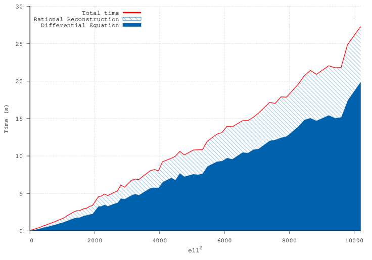
(a) $g=4$

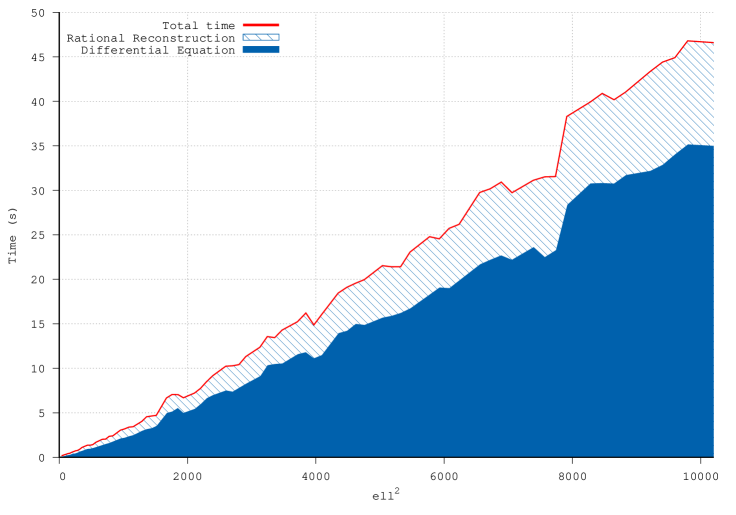
(b) $g=5$

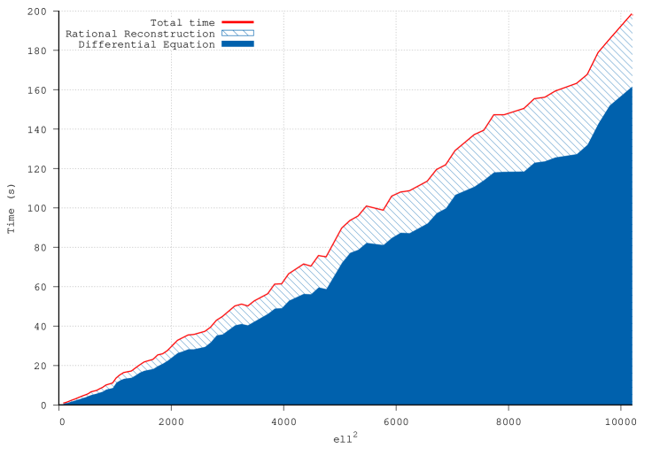
(c) $g=8$

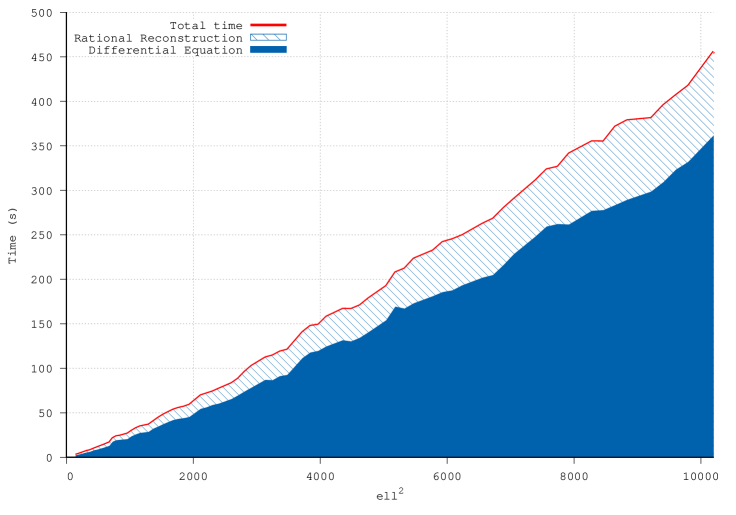
(d) $g=11$

Timings obtained with magma V2.25-7 on a laptop with an intel processor E5-2687WV4@3.00ghz

Figure 1: Computation of the multiplication-by-$\ell$ map over $\mathbb{F}_{5}$ for $\ell\in\{g+1,\ldots,101\}$ and such that gcd$(\ell,5)=1$

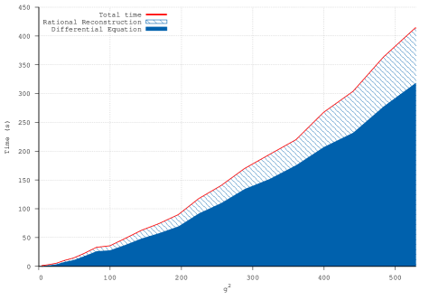
Timings obtained with magma V2.25-7 on a laptop with an intel processor E5-2687WV4@3.00ghz

Figure 2: Computation of the multiplication-by-$31$ map over $\mathbb{F}_{5}$ for $g\in\{2,\ldots,30\}$.

References

-
[1]
R. Schoof, Elliptic curves over finite
fields and the computation of square roots mod , Math. Comp. 44 (170)
(1985) 483–494.
doi:10.2307/2007968.
URL https://doi.org/10.2307/2007968 - [2] A. O. L. Atkin, The number of points on an elliptic curve modulo a prime, manuscript, Chicago IL (1988).
-
[3]
F. Morain, Calcul du nombre de
points sur une courbe elliptique dans un corps fini: aspects algorithmiques,
Journal de Théorie des Nombres de Bordeaux 7 (1) (1995) 255–282.
URL http://www.jstor.org/stable/43972443 -
[4]
R. Schoof, Counting points on
elliptic curves over finite fields, Journal de Théorie des Nombres de
Bordeaux 7 (1) (1995) 219–254.
URL www.numdam.org/item/JTNB_1995__7_1_219_0/ - [5] J. Pila, Frobenius maps of abelian varieties and finding roots of unity in finite fields, Mathematics of Computation 55 (1990) 745–763.
- [6] P. Gaudry, R. Harley, Counting points on hyperelliptic curves over finite fields, in: W. Bosma (Ed.), Algorithmic Number Theory, Springer Berlin Heidelberg, Berlin, Heidelberg, 2000, pp. 313–332.
- [7] P. Gaudry, É. Schost, Construction of secure random curves of genus 2 over prime fields, in: C. Cachin, J. L. Camenisch (Eds.), Advances in Cryptology - EUROCRYPT 2004, Springer Berlin Heidelberg, Berlin, Heidelberg, 2004, pp. 239–256.
-
[8]
S. Abelard, Counting points on
hyperelliptic curves with explicit real multiplication in arbitrary genus,
Journal of Complexitydoi:10.1016/j.jco.2019.101440.
URL https://hal.inria.fr/hal-01905580 -
[9]
A. Bostan, F. Morain, B. Salvy, E. Schost,
Fast algorithms for
computing isogenies between elliptic curves, Math. Comp. 77 (263) (2008)
1755–1778.
doi:10.1090/S0025-5718-08-02066-8.
URL https://doi.org/10.1090/S0025-5718-08-02066-8 - [10] P. Lairez, T. Vaccon, On -adic differential equations with separation of variables, in: Proceedings of the 2016 ACM International Symposium on Symbolic and Algebraic Computation, ACM, New York, 2016, pp. 319–323.
- [11] J.-M. Couveignes, T. Ezome, Computing functions on jacobians and their quotients, LMS Journal of Computation and Mathematics 18 (1) (2015) 555–577. doi:10.1112/S1461157015000169.
-
[12]
X. Caruso, E. Eid, R. Lercier,
Fast computation of
elliptic curve isogenies in characteristic two, working paper or preprint
(Mar. 2020).
URL https://hal.archives-ouvertes.fr/hal-02508825 -
[13]
E. Eid, Sur le calcul d’isogénies par
résolution d’équations différentielles p-adiques, Ph.D. thesis, thèse de
doctorat dirigée par Lercier, Reynald et Caruso, Xavier Mathématiques et
leurs interactions Rennes 1 2021 (2021).
URL http://www.theses.fr/2021REN1S012 -
[14]
J. Kieffer, A. Page, D. Robert,
Computing isogenies
from modular equations between Jacobians of genus 2 curves, working paper
or preprint (Jan. 2020).
URL https://hal.archives-ouvertes.fr/hal-02436133 -
[15]
R. Lercier, T. Sirvent,
On Elkies
subgroups of -torsion points in elliptic curves defined over a finite
field, J. Théor. Nombres Bordeaux 20 (3) (2008) 783–797.
URL http://jtnb.cedram.org/item?id=JTNB_2008__20_3_783_0 -
[16]
F. OORT, T. SEKIGUCHI, The
canonical lifting of an ordinary jacobian variety need not be a jacobian
variety, J. Math. Soc. Japan 38 (3) (1986) 427–437.
doi:10.2969/jmsj/03830427.
URL https://doi.org/10.2969/jmsj/03830427 -
[17]
X. Caruso,
Computations
with -adic numbers, Les cours du CIRM 5 (1).
doi:10.5802/ccirm.25.
URL https://ccirm.centre-mersenne.org/item/CCIRM_2017__5_1_A2_0 - [18] T. Vaccon, Précision p-adique: applications en calcul formel, théorie des nombres et cryptographie, Ph.D. thesis, University of Rennes 1 (2015).
-
[19]
K. S. Kedlaya, C. Umans, Fast
polynomial factorization and modular composition, SIAM J. Comput. 40 (6)
(2011) 1767–1802.
doi:10.1137/08073408X.
URL https://doi.org/10.1137/08073408X -
[20]
D. G. Cantor, On the analogue
of the division polynomials for hyperelliptic curves. 1994 (447) (1994)
91–146.
doi:doi:10.1515/crll.1994.447.91.
URL https://doi.org/10.1515/crll.1994.447.91 -
[21]
S. Abelard, Comptage de points de
courbes hyperelliptiques en grande caractéristique : algorithmes et
complexité, Ph.D. thesis, thèse de doctorat dirigée par Gaudry, Pierrick
et Spaenlehauer, Pierre-Jean Informatique Université de Lorraine 2018
(2018).
URL http://www.theses.fr/2018LORR0104 - [22] A. Bostan, F. Chyzak, M. Giusti, R. Lebreton, G. Lecerf, B. Salvy, É. Schost, Algorithmes efficaces en calcul formel, 2017.
-
[23]
X. Caruso, D. Roe, T. Vaccon,
Tracking -adic
precision, LMS J. Comput. Math. 17 (suppl. A) (2014) 274–294.
doi:10.1112/S1461157014000357.
URL https://doi.org/10.1112/S1461157014000357 - [24] X. Caruso, D. Roe, T. Vaccon, -adic stability in linear algebra, in: ISSAC’15—Proceedings of the 2015 ACM International Symposium on Symbolic and Algebraic Computation, ACM, New York, 2015, pp. 101–108.
- [25] J. S. Milne, Abelian varieties, in: Arithmetic geometry, Springer, 1986, pp. 103–150.
- [26] T. Matsusaka, On a characterization of a Jacobian variety, 1959.
- [27] A. Bostan, L. González-Vega, H. Perdry, É. Schost, From Newton sums to coefficients: complexity issues in characteristic , in: MEGA’05, 2005, eighth International Symposium on Effective Methods in Algebraic Geometry, Porto Conte, Alghero, Sardinia (Italy), May 27th – June 1st.
-
[28]
E. Kaltofen, L. Yagati,
Improved sparse multivariate
polynomial interpolation algorithms, in: Symbolic and algebraic computation
(Rome, 1988), Vol. 358 of Lecture Notes in Comput. Sci., Springer, Berlin,
1989, pp. 467–474.
doi:10.1007/3-540-51084-2\_44.
URL https://doi.org/10.1007/3-540-51084-2_44 - [29] E. Thomé, Algorithmes de calcul de logarithmes discrets dans les corps finis, Ph.D. thesis, École polytechnique (2003).
-
[30]
W. Bosma, J. Cannon, C. Playoust,
The Magma algebra system.
I. The user language, J. Symbolic Comput. 24 (3-4) (1997) 235–265,
computational algebra and number theory (London, 1993).
doi:10.1006/jsco.1996.0125.
URL http://dx.doi.org/10.1006/jsco.1996.0125 - [31] E. Eid, Package Equadif_Solver, https://github.com/eeid95/HyperellipticIsogeny (2022).