Towards Revenue Maximization with Popular and Profitable Products

Abstract.

Economic-wise, a common goal for companies conducting marketing is to maximize the return revenue/profit by utilizing the various effective marketing strategies. Consumer behavior is crucially important in economy and targeted marketing, in which behavioral economics can provide valuable insights to identify the biases and profit from customers. Finding credible and reliable information on products’ profitability is, however, quite difficult since most products tends to peak at certain times w.r.t. seasonal sales cycle in a year. On-Shelf Availability (OSA) plays a key factor for performance evaluation. Besides, staying ahead of hot product trends means we can increase marketing efforts without selling out the inventory. To fulfill this gap, in this paper, we first propose a general profit-oriented framework to address the problem of revenue maximization based on economic behavior, and compute the On-shelf Popular and most Profitable Products (OPPPs) for the targeted marketing. To tackle the revenue maximization problem, we model the $k$-satisfiable product concept and propose an algorithmic framework for searching OPPP and its variants. Extensive experiments are conducted on several real-world datasets to evaluate the effectiveness and efficiency of the proposed algorithm.

1. Introduction

Economic-wise, a common goal for companies conducting marketing is to maximize the return profit by utilizing various effective marketing strategies. Consumer behavior plays a very important role in economy and targeted marketing (Peng et al., 2012; Xu and Lui, 2016; Yang et al., 2016; Zhang and Chen, 2018). A successful business influences the behavior of consumers to encourage them buying its products. In marketing, behavioral economics can provide valuable insights via various web services, e.g., Amazon, by helping people to identify the biases and profit from all customers. On the other hand, manufacturers can use the information of consumers’ requirements on various products to select appropriate products in the market. As a result, evolving the ecosystem of personal behavioral data from web services has many real applications (Agrawal et al., 1994; Geng and Hamilton, 2006; Han et al., 2004; Quattrone et al., 2016). However, understanding consumer behavior is quite challenging, such as finding credible and reliable information on products’ profitability.

The consumer behavior analytics is crucially important for decision maker, which can be used to support the global market and has attracted many considerable attentions (Ahmed et al., 2009; Tseng et al., 2013; Peng et al., 2012; Xu and Lui, 2016; Yang et al., 2016). In economics, utility (Marshall, 2009) is a measure of a consumer’s preferences over alternative sets of goods or services. Specifically, only few works of data mining and information search have been studied (Teng et al., 2015; Quattrone et al., 2016; Xu and Lui, 2016; Zhang et al., 2016; Zhang and Chen, 2018), from a economic perspective, to study targeted marketing revenue/profit maximization based on economic behavior. Consider the consumer choice (Coleman and Fararo, 1992) and the preferences constraint, several crucial factors for the task of commerce has been succeeded (w.r.t. profit/utility maximization): i) rational behavior; ii) preferences are known and measurable; iii) inventory management; and iv) price. To obtain higher profit from the products, the decision-maker should find out the most profitable and popular products from the historical records. The reason is that the business people would likely know the amount of profit in their business, but it is, difficult to know which product makes the most money (Peng et al., 2012; Xu and Lui, 2016).

In recent decades, there are many studies have been proposed for computational economics which explores the intersection of economics and computation. In the same time, the scientists in field of computer science also incorporate some interesting concepts (e.g., utility theory) form Economics into various research domains, such as data mining, database, social network, Internet of Things, etc. In the field of data mining which also called knowledge discovery form data (KDD), there is tremendous interest in developing novel utility-oriented methodologies and models for obtaining insights over rich data. Therefore, a new utility-oriented data mining paradigm called utility mining (Tseng et al., 2013; Gan et al., 2018b, 2021) becomes an emerging technology and successfully be applied to various fields. For example, high-utility itemset mining (Tseng et al., 2013; Mai et al., 2017; Nguyen et al., 2019), high-utility sequence mining (Yin et al., 2012; Lan et al., 2014; Wang and Huang, 2018), and high-utility episode mining (Wu et al., 2013; Lin et al., 2015c) been extensively studied to deal with different types of data, including itemset-based transactional data, sequence data, and complex event data.

Most products operate on a seasonal sales cycle that tends to peak at a certain time in a year. How to sell the seasonal products to make profit maximization, the sale department can find what products are most likely purchased on special periods, by utilizing different seasonal consumer behavior data (i.e., weekly sales data, monthly sales data, quarterly sales data, and annual sales data). Despite On-Shelf Availability (OSA) is a key factor (Corsten and Gruen, 2003), out of stock levels on the shelf, as shown in Fig. 1, still remains highly persistent, and today’s economic environment is more challenging since it is even more critical than ever for retailers and manufacturers to ensure that every product a customer wants to buy is available every time. The historical data was analyzed to classify the groups of products and identify those are most likely to be sold-out first. A sustainable OSA management process should consider the frequency and quantity of ordering, as well as the inventory, to address the root causes of out-of-stocks. In general, the seasonal products may become popular/hot on some special periods. The popular/hot products that are flying off the shelves. For example, sunglasses may sold out during the summer, but for the coming up winter, fewer people would purchase it.

Figure 1. Out of stock products.

Product bundling is one of the sales strategy to make the successful commerce. Use product bundling to pair less profitable (even has negative profit) or slower-moving products with more profitable ones to reduce the storage savings of the less valuable products, which making more space to keep the products with higher profitability. To improve the overall business’ profitability, it is important to decide when and how to adjust product pricing and sell bundled products for further increasing profitability. Compared to the hot-sold out products, finding the most profitable products can increase the overall profitability (Ge et al., 2015). Ensuring most hot and profitable products on the shelf is essential for any retailer, but even today, it still remains a major challenge.

Motivated by existing research in economics, in this paper, we propose a profit-oriented framework to address the problem and compute the on-shelf popular and most profitable products for the targeted marketing. We also model $k$-satisfiable product searching and propose an algorithmic framework. The principle contributions of this paper are summarized as follows:

• This is the first work to systematically study the problem of computing on-shelf hot and most profitable products for the targeted marketing based on economic behavior, including purchase frequency, purchase time periodic, on-shelf availability and utility/profit theory. It can help us to make understand users’ economic behaviors, find out the On-shelf Popular and most Profitable Products (OPPPs), then make targeted marketing with profit maximization.

• The solution space of the designed approach can be reduced to a finite the number of points by tree-based searching technique. Two compact data structures are developed to store the necessary information of the databases.

• The concept of remaining positive profit is adopted to calculate the estimated upper bound. Based on developed pruning strategies, the OP3M algorithm can directly discover OPPPs using OPP-list with only twice database scans. Without the candidate generation-and-test, it performs a depth-first search by spanning the search space during the constructing process of the OPP-list.

• The extensive performance evaluation on several real-world e-commerce datasets demonstrates the effectiveness and efficiency of the proposed OP3M framework.

The rest of this paper is organized as follows. Some related works are reviewed in Section 2. The preliminaries and problem statement are given in Section 3. Details of the proposed OP3M algorithm are described in Section 4. The evaluation of the effectiveness and efficiency of the proposed OP3M framework are provided in Section 5. Finally, some conclusions are drawn in Section 6.

2. Related Work

Our research is related to the work in computational economic, utility-based mining, other profit-oriented searching and mining works. In particular, the advent of Internet has resulted in large sets of user behavior records, which makes it possible for targeted marketing to maximize the return profit. Up to now, evolving the ecosystem of personal behavioral data from web services has many real applications (Agrawal et al., 1994; Geng and Hamilton, 2006; Han et al., 2004; Quattrone et al., 2016; Fournier-Viger et al., 2017). For example, frequency-based pattern or rule mining (Agrawal et al., 1994; Han et al., 2004) is one of the common approaches to discover hidden relationships among items in the transaction. Different from the frequency-based mining model, the rare pattern mining framework that aim at discovering the non-frequent but interesting patterns also has been proposed (Koh and Ravana, 2016). Geng and Hamilton (Geng and Hamilton, 2006) reviewed some measures that are intended for selecting and ranking patterns according to the potential interest to the user. The consumer behavior analytics is crucially important for decision-maker, which can be used to support the global market and has attracted many considerable attentions (Tseng et al., 2013; Peng et al., 2012; Xu and Lui, 2016; Yang et al., 2016). Recently, some researchers studied the profit of web mining such as profit-oriented pattern mining (Ahmed et al., 2009; Tseng et al., 2013), association (Yang et al., 2007), market share (Quattrone et al., 2016), and decision making to maximize the revenue from products (Agrawal et al., 1994; Geng and Hamilton, 2006; Teng et al., 2015). Periodicity is prevalent in physical world, and many events involve more than one periods. The previous profit-oriented works (Liu et al., 2005; Tseng et al., 2013) and skyline operator (Ugarte et al., 2017) have not yet optimized to handle temporal on-shelf data, on-shelf availability (Corsten and Gruen, 2003), even considering both positive and negative unit profits. In this class of data regarding time, the period of interest needs to be added as an additional constraint to be evaluated together with the decision criteria of the addressed problem.

In economics, utility (Marshall, 2005) is a key measure of a consumer’s preferences over alternative sets of goods or services. It is a basic building block of rational choice theory (Coleman and Fararo, 1992). Up to now, some works that exploring the economic behavior data have been studied (Teng et al., 2015; Quattrone et al., 2016; Xu and Lui, 2016; Zhang et al., 2016), from the data mining and information search perspectives. For example, considering the utility concept, a new data mining paradigm called utility mining (Tseng et al., 2013; Gan et al., 2018b, 2021; Mai et al., 2017; Wang and Huang, 2018) has been extensively studied and applied to different applications. Although a straightforward enumeration of all high-utility patterns (HUPs) sounds promising, it unfortunately does not yield a scalable solution for utility computation of patterns. The reason is that utility in HUPs does not hold the well-known Apriori property (Agrawal et al., 1994) (aka the downward closure property (Agrawal et al., 1994)) (Ahmed et al., 2009; Tseng et al., 2013; Gan et al., 2018b, 2021). Utility mining has been extended to deal with different types of data, including itemset-based transactional data (Tseng et al., 2013; Mai et al., 2017), sequence data (Yin et al., 2012; Lan et al., 2014; Wang and Huang, 2018), uncertain data (Lin et al., 2016c, 2017), and complex event data (Wu et al., 2013; Lin et al., 2015c). Furthermore, various interesting and challenging issues about utility mining have been addressed, including top-$K$ high-utility pattern mining (Tseng et al., 2016; Duong et al., 2016; Yin et al., 2013), utility mining in dynamic databases (Lin et al., 2015b, 2016b; Gan et al., 2018b), mining high-utility patterns by taking different special constraints into account (Lin et al., 2015a, 2016d; Lan et al., 2015; Nguyen et al., 2019), and privacy preserving utility mining (Gan et al., 2018a), etc. Overall, utility-driven pattern mining has been shown to be of considerable value in a wide range of applications.

There are many heuristic search algorithms in artificial intelligence such. Up to now, there has been several studies about heuristic search (Guns et al., 2011c), constraint programming (Guns et al., 2011a, b), and multi-objective optimization (Ugarte et al., 2017) such as Pareto for pattern mining. Notice that exhaustive search strategy explores many possible subsets, while heuristic search strategy explores a limited number of possible subsets. Thus, they are different. In particular, in heuristic search methods, the state space is not fully explored and randomization is often employed. Most of the studies of utility mining and pattern mining aim at discovering an optimal set of interesting patterns under the given constraints, while some approaches may lead to not necessarily optimal result by the heuristic search.

In other related research fields, some interesting works have applied the utility theory (Marshall, 2005) to recommender systems (Li et al., 2011; Wang and Zhang, 2011; Ying et al., 2014; Zhang and Chen, 2018). Wang and Zhang (Wang and Zhang, 2011) first incorporates marginal utility into product recommender systems. They adapt the widely used Cobb-Douglas utility function (Coleman and Fararo, 1992) to model product-specific diminishing marginal return and user-specific basic utility to personalize recommendation. Li et al. (Li et al., 2011) highlights that product recommender systems differ from the music or movie recommender systems as the former should take into account the utility of products in their ranking. It employs the utility and utility surplus (Zhang and Chen, 2018) theories from economics and marketing to improve the list of recommended product. (Zhao et al., 2017) finds multi-product utility maximization for economic recommendation. These existing product recommender systems, however, do not consider the time periodicity between the products purchased and on-shelf availability. The work in (Zhao et al., 2012) utilizes the purchase interval information to improve the performance for e-commerce, but it does not consider the on-shelf availability and purchase frequency of products.

3. Preliminaries and Problem Formulation

3.1. Utility-based Computing Model

A fundamental notion in utility theory is that each consumer is endowed with an associated utility function, which is “a measure of the satisfaction from consumption of various goods and services” (Marshall, 2009). In the context of purchasing decisions, we assume that the consumer has access to a set of products, each product having a price. Informally, buying a product involves the exchange of money for a product. Given the utility of a product, to analyze consumers’ motivation to trade money for the product, it is also necessary to analyze consumer behavior. In economics, the utility that a consumer has for a product can be decomposed into a set of utilities for each product characteristic. According to this utility theory, we have the following concepts and formulation. The notations of symbols are first summarized in Table 1.

Table 1. Summary of Notations

Symbol	Description
$I$	A set of $m$ items/products, I = {i1, i2, $\ldots$, im}.
$X$	A group of products $X$ = $\{i_{1},$ $i_{2},$ $\dots,i_{j}\}$.
$D$	A quantitative database, D = {T1, T2, $\ldots$, Tn}.
minfre	A minimum frequent threshold.
minpro	A minimum profit threshold.
$sup(X)$	The total support value of $X$ in $D$.
OPPP	On-shelf most popular and profitable product.
$q(i_{j},T_{c})$	The occurred quantity of an item $i_{j}$ in $T_{c}$.
$up(i_{j})$	Each item $i_{j}\in I$ has a unit profit.
$p(i_{j},T_{c})$	The profit of an item $i_{j}$ in $T_{c}$.
$p(X,h)$	The sum of profits of $X$ in a period $h$.
RTWU	Redefined transaction-weighted utilization.
pp(X)	The sum of positive profit of $X$ in $D$.
np(X)	The sum of negative profit of $X$ in $D$.
rpp(X)	The sum of remaining positive profit of $X$ in $D$.
OPP-list	List structure with On-shelf Popularity and Profit.
OFU±-table	An On-shelf Frequency-Utility (with both positive
	and negative profit value) table.
X.list	The OPPP-list of a group of product $X$.

Example 3.1.

Consider an e-commerce database shown in Table 2, which will be used as running example in the following sections. Similar to the e-commerce database provided by RecSys Challenge 2015 (it contains some negative profit values since many all-occasion gifts are sold.), this example database contains five purchase behavior records ($T_{1},T_{2},\dots,T_{5}$) and three time periods ($1,2,3$). Behavior $T_{1}$ occurred in time period 2, and contains products $b$, $c$, and $e$, which respectively appear in $T_{1}$ with a purchase quantity of 2, 1 and 3. Table 3 indicates that the external profit w.r.t. unit profit of these products are respectively -$2, $4 and $7. Notice that the negative unit profit of a product $b$ indicates that this product is sold at a loss.

Table 2. An e-commerce database

Tid	User	Purchase record	Period
$T_{1}$	$U_{1}$	$(b,2)(c,1)(e,3)$	1
$T_{2}$	$U_{2}$	$(a,1)(b,1)(c,2)(f,1)$	1
$T_{3}$	$U_{3}$	$(a,3)(b,6)(c,4)(d,1),(e,1),(f,2)$	2
$T_{4}$	$U_{4}$	$(c,3)(d,3)(e,1)$	2
$T_{5}$	$U_{5}$	$(a,1)(d,2)(e,3)(f,1)$	3

Given a time-varying e-commerce database such that $D$ = {$T_{1}$, $T_{2}$, $\dots$, $T_{n}$} containing a set of temporal consumer purchase behaviors. Each transaction $T_{c}$ is a behavior record of one consumer, $T_{c}$ $\in D$ is a subset of $I$, and $T_{c}$ has a unique identifier $c$ called its Tid. Let $I$ be a set of distinct products/items, $I$ = {$i_{1}$, $i_{2}$, $\dots$, $i_{m}$}. Each product/item $i_{j}\in I$ is associated with a positive or negative number $up(i_{j})$, called its unit profit. For each transaction $T_{c}$ such that $i_{j}$ $\in$ $T_{c}$, a positive number $q(i_{j}$, $T_{c})$ is called purchase quantity of $i$. Let PE be a set of positive integers representing time periods, for any given period, this could be a weekly, monthly, quarterly or yearly timespan. Note that each transaction $T_{c}\in D$ is associated to a time period $pe(T_{c})\in PE$, representing the duration time in a period, which the transaction occurred.

In general, the profit of $X\subseteq I$ is associated to the cost price and selling price. For the addressed problem in this paper, assume that the unit profit of each distinct product has been given in the pre-defined profit-table, as shown in Table 3. As mentioned before, it is usually seen in cross-promotion with negative profits. Although giving away a unit of product $\{b\}$ results in a loss of $4 for the supermarket, selling bundled products $\{(c,1)(e,3)\}$ that are cross-promoted with $\{b\}$ generates $21 profit.

Table 3. External profit values (unit profit)

Product	$a$	$b$	$c$	$d$	$e$	$f$
Profit ($)	3	-2	4	1	7	5

Given a set of products $I$ and a set of customers $C$ = {$c_{1}$, $c_{2}$, $\dots$, $c_{j}$}, the market contribution of a group of products $X$ = {$i_{1}$, $i_{2}$, $\dots$, $i_{j}$} is related to the profit from $X$ after marketing. Finally, the contribution of a group of products $X$ becomes the sum of the profits it receives from all the customers in the market. Therefore, the key concepts used in this paper are first introduced as follows. A utility function is a map $U$: $X\longrightarrow\Re$. The profit of a combined product $X$ (a group of products $X\subseteq I$) in a transaction $T_{c}$ is:

(1) $$p(X,T_{c})=\sum_{i_{j}\in X\wedge X\subseteq T_{c}}{p(i_{j},T_{c})}.$$

where $p(i_{j},T_{c})$ is the profit of a product $i_{j}\in I$ in a transaction $T_{c}$, and $p(i_{j},T_{c})$ can be calculated as $p(i_{j},T_{c})$ = $up(i_{j})$ $\times$ $q(i_{j},T_{c})$. It represents the profit generated by products $i\in X$ in $T_{c}$. Consider the set of time periods where $X$ was sold, the time periods (on-shelf time) of a group of products $X\subseteq I$ becomes $os(X)$ = $\{pe(T_{c})|T_{c}\in D$ $\wedge X$ $\subseteq T_{c}\}$. Let $p(X,h)$ denote the profit of a group of products $X\subseteq I$ in a time period $h\in os(X)$, then by Eq. (2) we have:

(2) $$p(X,h)=\sum_{T_{c}\in D\wedge h\in os(X)}{p(X,T_{c})}.$$

By Eq. (3) we have the overall profit of a group of products $X\subseteq I$ in an e-commerce database $D$ as $p(X)$ = $\sum_{h\in os(X)}{p(X,h)}$. Thus, given a group of products $X$, let $top(X)$ denote the total profit of the time periods about $X$, then it can be represented in a function as follows:

(3) $$top(X)=\sum_{h\in os(X)\wedge T_{c}\in D}{tp(T_{c})},$$

where $tp(T_{c})$ is the transaction profit (tp) of a transaction $T_{c}$, i.e.,

(4) $$tp(T_{c})=\sum_{i\in T_{c}}{p(i,T_{c})}.$$

Let $rp(X)$ denote the relative profit of a group of products $X\subseteq I$ in an e-commerce database $D$, by Eq. (4) we have $rp(X)$ = $p(X)$/$top(X)$, and it represents the percentage of the profit that was generated by $X$ during the time periods where $X$ was sold.

Example 3.2.

The profit of product $e$ in $T_{1}$ is $p(e,T_{1})$ = 3 $\times$ $7 = $21, and the profit of products $\{c,e\}$ in $T_{1}$ is $p(\{c,e\},T_{1})$ = $p(c,T_{1})$ + $p(e,T_{1})$ = 1 $\times$ $4 + 3 $\times$ $7 = $25. The time periods of $\{c,e\}$ are $os(\{c,e\})$ = {period 1, period2}. The profit of $\{c,e\}$ in periods 1 and 2 are respectively $p(\{c,e\}$, period 1) = $25, and $p(\{c,e\}$, period 2) = $42. The profit of $\{c,e\}$ in the database is $p(\{c,e\})$ = $p(\{c,e\}$, period 1) + $p(\{c,e\}$, period 2) = $25 + $42 = $67. The transaction profit of $T_{1}$, $T_{2}$, $\dots$, $T_{5}$ are $tp(T_{1})$ = $21, $tp(T_{2})$ = $14, $tp(T_{3})$ = $31, $tp(T_{4})$ = $20 and $tp(T_{5})$ = $31. The total profit of the time periods of $\{c,e\}$ is $top(\{c,e\})$ = $tp(T_{1})$ + $tp(T_{3})$ + $tp(T_{4})$ = $72. The relative profit of $\{c,e\}$ is $rp(\{c,e\}$ = $p(\{c,e\})$/$top(\{c,e\})$ = $67 / $72 = 0.93.

3.2. On-Shelf Availability

On-Shelf Availability (OSA) (Corsten and Gruen, 2003) is a key factor of product for sale to the customer. It is impacted by a host of different factors, all along with the supply chain. Out of Stock (OOS) (Corsten and Gruen, 2003) is also known as stock-out, it is a situation where the retailer does not physically possess a particular product category, on its shelf, to sell this product to the customer. It can be estimated from store inventory data.

The retail industry being the highly competitive field, being able to fulfill customer expectations and the demands has become the most essential element in order to get sustainable growth and profit margin. Among them, on-shelf availability plays a key indicator for the retail industry, which can greatly impact the profit and customer loyalty. On the basis of the dataset shown in Table 2, and by taking the OSA, popularity and profit into account as the primary decision criteria, details of each product are shown in Table 4.

Table 4. Details of each product

Product	Profit	Quantity	Seasonal period
			Start	End
$a$	$12	4	1	3
$b$	-$18	9	1	2
$c$	$40	10	1	2
$d$	$6	6	2	3
$e$	$56	8	1	3
$f$	$20	4	1	3

Let $sup(h)$ denote the frequency of a time period $h$ w.r.t. $sup(h)$ = $|$the number of ${T_{c}\in h}|$, and $sup(X,h)$ denote the number of $|X\subseteq T_{c}\wedge T_{c}\in h|$, then the relative frequency of a group of products $X$ for a time period $h$ can be defined as:

(5) $$rf(X,h)=sup(X,h)/sup(h).$$

Consider products $\{c\}$ and $\{a,c\}$ in period 1, $sup(\textit{period}1)$ = 2, thus $rf(\{c,\textit{period}1\})$ = $2/2$ = 1.0, and $rf(\{a,c\},\textit{period}1)$ = $1/2$ = 0.5. Besides, $rf(\{c,\textit{period}1\})>$ $rf(\{a,c\},\textit{period}1)$. The relative profit of a group of products $X$ for a time period $h$ is

(6) $$rp(X,h)=p(X,h)/top(h),$$

where $top(h)$ means the total profit of a time period $h$, and $top(h)=\sum_{T_{c}\in h\wedge T_{c}\in D}{tp(T_{c})}$. Consider products $\{c\}$ and $\{a,c\}$ in period 1, $top(\textit{period}1)$ = $tp(T_{1})$ + $tp(T_{2})$ = $21 + $14 = $35, thus $rp(\{c,\textit{period}1\})$ = $12$/$$35 = 0.343, and $rp(\{a,c\},\textit{period}1)$ = $11$/$$35 = 0.314.

3.3. Problem Formulation

A group of products $X$ is said to be the on-shelf most popular and profitable products (OPPP) if it is popular in one or more periods $pt$ (its occurred relative frequency is no less than a user-specified minimum frequent threshold $minfre$), and it is high profitable in $pt$ (its relative profit $rp(X)$ is no less than a user-specified minimum profit threshold $minpro$ given by the user $(0\leq minpro\leq 1)$. Otherwise, $X$ is a non-OPPP.

For clarity, when we use the terms of “OPPP”, which indicates “On-shelf most Popular and Profitable Product”. The OPPP makes maximal profit with various customer satisfactions in terms of on-shelf period, high popular and high profitable products. Thus, the significant concept of OPPP is actually a $k$-satisfiable product. If a product satisfies at least $k$-constraints (i.e., OSA constraint, popular w.r.t. inventory control, high profitable product), we say that this product is $k$-satisfiable product for maximizing profit where $k$ is a user’s predefined parameter and a non-negative integer. In the addressed OP3M problem and the given running example, $k$ is equal to 3. To satisfy the customers, retailers must be able to obtain to their feedback and improve the services. Regarding to the above analytics, the decision maker can make the efficient business strategy and decision, which can improve the overall profitability in his/her business. Ensuring the on shelf product is essential for any retailer, but even today it remains a major challenge.

Problem statement. The problem by computing the most popular on-shelf and profitable products for the targeted marketing is to discover all significant OPPPs in an e-commerce database containing unit profit values are positive. The problem by computing the most popular on-shelf and profitable products for targeted marketing with negative values is to discover all OPPPs in an e-commerce database where external unit profit values are positive or negative.

A naive way for this problem is to enumerate all possible subsets of products $I$, then calculate the sum of the frequency and profits of each possible subset, and choose the frequent subsets with the highly sum profit. However, this approach is not scalable because there is an exponential number of all possible subsets. This motivates us to propose an efficient algorithm named OP3M for the searching problem of OPPPs. For efficient multi-criteria decision analyses, as mentioned previously, we can utilize heuristic search (Guns et al., 2011c), constraint programming (Guns et al., 2011a, b), and multi-objective optimization (Ugarte et al., 2017). An alternative approach is to formulate a truly multi-objective optimization problem where the heuristic search tries to optimize for each criterion with respect to each other. However, the state space of heuristic search methods is not fully explored and randomization is often employed. Therefore, OP3M utilizes exhaustive search strategy with various user-specified constraints instead of heuristic search. Overall, OP3M is an exact utility-based framework but not a randomize one.

4. The Proposed OP3M Algorithm

4.1. Properties of On-Shelf Availability

It can be demonstrated that the popularity measure is anti-monotonic (Agrawal et al., 1994; Ugarte et al., 2017), any superset of a non-popular pattern cannot be a popular pattern, while (relative) profit measure is not monotonic or anti-monotonic (Liu et al., 2005; Tseng et al., 2013). In other words, a product may have a lower, equal or higher profit than that of the profit of its subsets. We extend the concept of transaction-weighted utilization (TWU) (Liu et al., 2005; Ahmed et al., 2009) in OPPP to show properties of on-shelf availability. For a given time period $h$, let $\textit{RTWU}(X,h)$ denote the redefined transaction-weighted utilization of a group of products $X$ in $h$, thus it is the sum of the redefined transaction profit of transactions from $h$ containing $X$.

To handle the negative profit of product, the redefined transaction-weighted utilization (RTWU) (Lin et al., 2016a) of a group of products $X$ is defined as:

(7) $$\textit{RTWU}(X)=\sum_{T_{c}\in D\wedge X\subseteq T_{c}}{rtp(T_{c})}.$$

where $rtp(T_{c})$ is the redefined transaction profit (abbreviated as rtp) of a transaction $T_{c}$, that is $rtp(T_{c})$ = $\sum_{x\in T_{c}\wedge p(x)>0}{p(X,T_{c})}$. Thus, $rtp(T_{c})$ contains the sum of the positive profit of the products in $T_{c}$, while negative external profits are ignored. Similarly, the redefined transaction-weighted utilization of a group of products $X$ for a time period $h$ can be represented as:

(8) $$\textit{RTWU}(X,h)=\sum_{T_{c}\in D\wedge X\subseteq T_{c}\wedge pe(T_{c})\subseteq h}{rtp(T_{c})}.$$

For the running example (considering that $b$ has an external profit value of $-\$2$), the rtp of $T_{1}$, $T_{2}$, $T_{3}$, $T_{4}$, and $T_{5}$ are respectively $25, $16, $43, $20 and $31. The RTWU of products $a$, $b$, $c$, $d$, $e$, and $f$ are respectively $90, $84, $104, $94, $119 and $90. With reflexivity of OSA makes sense at all, the continuous utility function has several components, and the addressed problem becomes quite complicated. According to previous studies (Lin et al., 2016a; Fournier-Viger and Zida, 2015), we generalize the properties of on-shelf availability for the case of an e-commerce database with time-sensitive periods as follows.

Property 1.

The RTWU of a group of products $X$ for a period $h$ is an upper bound on the profit of $X$ in period $h$, that is $\textit{RTWU}(X,h)$ $\geq$ $p(X,h)$.

Property 2.

The RTWU measure is anti-monotonic in the whole database or in a specific period. Let $X$ and $Y$ be two products, if $X\subset Y$, then $\textit{RTWU}(X)$ $\geq$ $\textit{RTWU}(Y)$; for a period $h$, it has $\textit{RTWU}(X,h)$ $\geq$ $\textit{RTWU}(Y,h)$.

Property 3.

Let $X$ be a group of products, if $\textit{RTWU}(X)$/$top(X)$ $<$ minpro, then the product $X$ is low profit as well as all its supersets.

Property 4.

The RTWU of a group of products $X$ divided by the total profit of its time periods $h$ is higher than or equal to its relative profit in periods $h$, i.e., $\textit{RTWU}(X,h)$ / $top(X)$ $\geq$ $rp(X,h)$. It is an upper bound on the relative profit of a group of products.

Property 5.

Given a group of products $X$, if there does not exist a time period $h$ such that $\textit{RTWU}(X,h)$/$top(X)$ $\geq$ minpro, then $X$ is not an profitable on-shelf product. Otherwise, $X$ may or may not be an profitable on-shelf product.

Consider products $\{c\}$ and $\{a,c\}$ in period 1, the values $\textit{RTWU}(\{c\})$ and $\textit{RTWU}(\{a,c\})$ are $90 and $59, which are the overestimations of $p(\{a\})$ = $39 and $p(\{a,c\})$ = $36, thus respecting Property 4. Suppose the above properties we’ve been studying, and the previous proposition true, we still cannot easily solve the OP3M problem.

4.2. Properties of Positive and Negative Profits

Economic profit can be positive, negative, or zero. If your business generates a negative profit, this means that, for the time those products are sold less than their cost price. Thus, some products went less successful than others and got negative profit. Nevertheless, all profit together make a whole profit for each cosmetic product, which is common seen in the successful business. What if the profit target is negative and the final actual result is positive? The following properties hold.

First, let the total order $\prec$ on products in the designed algorithm adopts the RTWU ascending order of products, and negative products always succeed all positive products. In the running example, the RTWU of six products $a$, $b$, $c$, $d$, $e$, and $f$ are respectively as $90, $84, $104, $94, $119, and $90, thus the total order $\prec$ on products is $a\prec$ $f\prec$ $d\prec c$ $\prec e\prec b$. The complete search space of the addressed problem can be represented by a Set-enumeration tree (Rymon, 1992) where products are sorted according to the previous total order $\prec$. By utilizing the OPP-list and OFU^±-table, we named this tree as OPP-tree. In this OPP-tree, according to the total order $\prec$, all child nodes of any tree node are called its extension nodes. For any products (product-sets) $X$, let $pp(X)$ and $np(X)$ respectively denote the sum of positive profits and the sum of negative profits of $X$ in a transaction or period or database, such that $p(X)$ = $pp(X)$ + $np(X)$. We have the following important observations.

Property 6.

Relationship between positive profits and negative profits of a group of products: $np(X)$ $\leq p(X)$ $\leq pp(X)$ in a transaction or period or database (Lin et al., 2016a). We respectively denote as $np(X,T_{c})$ $\leq p(X,T_{c})$ $\leq$ $pp(X,T_{c})$ in a transaction $T_{c}$, $np(X,h)$ $\leq$ $p(X,h)$ $\leq$ $pp(X,h)$ in a period $h$, and $np(X)$ $\leq$ $p(X)$ $\leq$ $pp(X)$ in a database.

It can be seen that the positive profit value of a group of products is always no less than its actual profit, while the negative profit value is just the opposite. Thus, the positive profit value is an upper-bound on the profit. However, both $pp(X)$ and $np(X)$ cannot be used to overestimate the profit of a group of products. As an upper-bound on profit, $pp(X)$ still does not hold the downward closure property for the extensions with positive or negative products.

4.3. OPP-List and OFU^±-Table

In this subsection, we introduce the new concept called “list structure of a group of products with its On-shelf Popularity and Profit” (OPP-list for short) which is a component used for the information storing and calculation. Besides, a new concept called remaining positive profit is introduced and applied to obtain the estimated upper-bound, which will be presented in next subsection. First, the OPP-list structure is defined as follows.

Definition 4.1.

Let $rpp(X,T_{c})$ denote the remaining positive profit of a group of products $X$ in a transaction $T_{c}$. Thus, $rpp(X,T_{c})$ is the sum of the positive profit values of each product appearing after $X$ in $T_{c}$ according to the total order $\prec$. It is represented as:

(9) $$rpp(X,T_{c})=\sum_{i_{j}\notin X\wedge X\subseteq T_{c}\wedge X\prec i_{j}}p(i_{j},T_{c}),p(i_{j},T_{c})\geq 0.$$

Definition 4.2.

The OPP-list in an e-commerce database $D$ is a set of tuples corresponding to the transactions where $X$ appears. A tuple is defined as $<$$\underline{tid}$, $\underline{pp}$, $\underline{np}$, $\underline{rpp}$, period $>$ for each transaction $T_{c}$ containing $X$.

• $\underline{tid}$: the transaction identifier of $T_{c}$;

• $\underline{pp}$: the positive profit of $X$ in $T_{c}$, i.e., $p(X,T_{c})\geq 0$;

• $\underline{np}$: the negative profit of $X$ in $T_{c}$, i.e., $p(X,T_{c})<0$;

• rpp: the remaining positive profit of $X$ in $T_{c}$, w.r.t. $rpp(X,T_{c})$;

• period: the related period where $T_{c}$ is occurred.

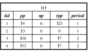
Figure 2. Constructed OPP-lists of product ($c$).

Example 4.3.

Since the total order $\prec$ on products is $a\prec f\prec d\prec c\prec e\prec b$, we have that $rpp(a,T_{3})$ = $p(f,T_{3})$ + $p(d,T_{3})$ + $p(c,T_{3})$ + $p(e,T_{3})$ = $10 + $1 + $16 + $67 = $34, and $rpp(\{a,c\},T_{3})$ = $p(e,T_{3})$ = $7. Thus, the OPP-list of product $(c)$ is $\{(T_{1}$, $4, 0, $21, 1), $(T_{2}$, $3, 0, 0, 1), $(T_{3}$, $16, 0, $7, 2), $(T_{4}$, $12, 0, $7, 2), $\}$, as shown in Fig. 2. It can perform a single database scan to create the all OPP-lists of all 1-products in the processed database. Based on the designed OPP-list and previous studies (Lin et al., 2016a; Fournier-Viger and Zida, 2015), we can extract the following information.

For a group of products X, let $pp(X,h)$, $np(X,h)$, and $rpp(X,h)$ are respectively the sum of pp values, the sum of np values and the sum of rpp values in a period $h$ w.r.t. OPP-list of X, that are:

(10) $$pp(X,h)=\sum_{X\subseteq T_{c}\wedge T_{c}\in h}pp(X,T_{c});$$

(11) $$np(X,h)=\sum_{X\subseteq T_{c}\wedge T_{c}\in h}np(X,T_{c});$$

(12) $$rpp(X,h)=\sum_{X\subseteq T_{c}\wedge T_{c}\in h}rpp(X,T_{c}).$$

Similarly, let $pp(X)$, $np(X)$, and $rpp(X)$ are respectively the sum of pp values, the sum of np values and the sum of rpp values for a group of products X in the database $D$ w.r.t. OPP-list of X, we have:

(13) $$pp(X)=\sum_{X\subseteq T_{c}\wedge T_{c}\in D}pp(X,T_{c});$$

(14) $$np(X)=\sum_{X\subseteq T_{c}\wedge T_{c}\in D}np(X,T_{c});$$

(15) $$rpp(X)=\sum_{X\subseteq T_{c}\wedge T_{c}\in D}rpp(X,T_{c}).$$

By utilizing the property of OPP-list, we further design a structure called on-shelf frequency-profit table with both positive and negative value, hereafter termed OFU^±-table. The OFU^±-table of a pattern is built after the construction of its OPP-list, and it stores the following information.

Definition 4.4.

An OFU^±-table of a group of products $X$ contains nine parts: (1) name: the name of product $X$; (2) sup(X, h): the support of $X$ in a period $h$; (3) sup(X): the support of $X$ in database $D$; (4) pp(X, h): the summation of the positive profits of $X$ in a period $h$; (5) pp(X): the summation of the positive profits of $X$ in database $D$; (6) np(X, h): the summation of the negative profits of $X$ in a period $h$; (7) np(X): the summation of the negative profits of $X$ in database $D$; (8) rpp(X, h): the summation of the remaining positive profits of $X$ in $h$; and (9) rpp(X): the summation of the remaining positive profits of $X$ in $D$. Notice that there is a HashMap to respectively keep the sup(X, h), pp(X, h), np(X, h) and rpp(X, h) vaules of product $X$ in each period $h$.

Example 4.5.

The construction process of a OFU^±-table is as follows. Consider a group of products $(c)$ in Table 2, it appears in $T_{1}$, $T_{2}$, $T_{3}$, and $T_{4}$. From the built OPP-list of $(c)$ which is shown in Fig. 2, the OFU^±-table of product $(c)$ is efficiently constructed using the support count, positive profit, negative profit and remaining positive profit. They are calculated during the construction of its OPP-list, and the results of its OFU^±-table are {$sup(c)$ = 4, $pp(c,1)$ = $7, $pp(c,2)$ = $28, $pp(c)$ = $pp(c,1)$ + $pp(c,2)$ = $35, $np(c,1)$ = $np(c,2)$ = $np(c)$ = $0, and $rpp(c,1)$ = $21, $rpp(c,2)$ = $14, $rpp(c)$ = $rpp(c,1)$ + $rpp(c,2)$ = $35}.

After initially constructing the OPP-list and OFU^±-table of each 1-product/item, for any $k$-product ($k\geq 2$), its’ OPP-list can be directly calculated using the OPP-lists of some of its subsets, without scanning the database. The construction procedure of the OPP-list and OFU^±-table of a $k$-product, and is shown in Algorithm 1. Let be a product $X$ and two products $X_{a}$ and $X_{b}$, they are extensions of $X$ by respectively adding two distinct products $a$ and $b$ to $X$. The construction procedure takes as input the OPP-lists of $X$, $X_{a}$ and $X_{b}$, and outputs the OPP-list and OFU^±-table of the pattern $X_{ab}$. Specially, it is important to notice that the construction for $k$-product ($k\geq 3$, Lines 4 to 7) is different from that of $k$-product ($k$ = 2, Line 9). For instance, the profit value of {$a,b$} is the sum profit value of {$a$} and {$b$}. And the 3-itemset {$a,b,c$} its OPP-list is constructed by the OPP-lists of {$a,b$} and {$b,c$}, and the sum profit value of {$a,b$} and {$b,c$} has a duplicate profit value of {$b$}. Thus, it should avoid duplication for $k$-product ($k\geq 3$). It can be easily implemented, because the all necessary information of ($k$-1)-product ($k\geq 2$) has been calculated before constructing the OPP-list of $(k)$-product ($k\geq 2$) w.r.t. the extension pattern.

Input: $X$, $X_{a}$, $X_{b}$.

Output: $X_{ab}$.

1 set $X_{ab}.list\leftarrow\emptyset$, $X_{ab}.table$ $\leftarrow\emptyset$;

2 for each tuple $E_{a}\in X_{a}.list$ do

3       if $\exists E_{a}\in$ $X_{b}.list$ $\wedge E_{a}.tid$ == $E_{b}.tid$ then

4             if $X.list\neq\emptyset$ then

5                   Search for element $E\in X.list$, $E.tid$ = $E_{a}.tid$;

6                   $E_{ab}\leftarrow<E_{a}.tid$, $E_{a}.pp$ + $E_{b}.pp$ - $E.pp$, $E_{a}.np$ + $E_{b}.np$ - $E.np$, $E_{b}.rpp$, $E_{a}.\textit{period}>$;

7                  

8             end if

9            else

10                   $E_{ab}\leftarrow<E_{a}.tid$, $E_{a}.pp$ + $E_{b}.pp$, $E_{a}.np$ + $E_{b}.np$, $E_{b}.rpp$, $E_{a}.\textit{period}>$;

11                  

12             end if

13            $X_{ab}.list$ $\leftarrow$ $X_{ab}.list$ $\cup E_{ab}$;

14             update information in the OPP-table for $X_{ab}$;

15            

16       end if

17      

18 end for

return $X_{ab}$ 

ALGORITHM 1 Construction procedure

4.4. Filtering Strategies for Searching

Lemma 4.6.

(Anti-monotonicity of the unpromising product with support). In the search space w.r.t. OPP-tree, if a tree node is a popular product in the whole database $D$ or a period $h$, its parent node is also a popular product in $D$ or $h$. Let $X$ be a $k$-products (node) and its parent node are denoted as $X^{\prime}$, a ($k$-1)-products. For a given database $D$ or a period $h$, the relative frequency measure is anti-monotonic: $rf(X)\leq rf(X^{\prime})$ always holds.

Proof.

According to well-known Apriori property (Agrawal et al., 1994), it always exists the relationship $sup(X,h)$ $\leq$ $sup(X^{\prime},h)$. Thus, the downward closure property of relative frequency measure can be hold. ∎

Lemma 4.7.

(Anti-monotonicity of unpromising product with profit upper-bound). For any node $X$ in the search space w.r.t. the OPP-tree, the sum of $\textit{SUM}(X.pp)$ and $\textit{SUM}(X.rpp)$ in the OPP-list of $X$ (within a period or the whole database) is larger than or equal to profit of any one of its children (within any period $h$ or the whole database $D$ w.r.t. the whole/maximal period in database).

Thus, there exists an upper bound on profit of any pattern/node with respect to a special period. Lemma 4.7 guarantees that the sum of profits of $X$ in $D$ or $h$ w.r.t $p(X)$ is always less than or equal to the sum of SUM$(X^{\prime}.pp)$ and SUM$(X^{\prime}.rpp)$ in $D$ or $h$. It ensures that the downward closure property of transitive extensions with positive or negative products, based on these observations, we can use the following two filtering strategies.

Strategy 1.

When performing a depth-first search strategy on the OPP-tree, if the relative frequency of any product $X$ within a time period $h$ is less than minfre (w.r.t. $rf(X,h)$ = $sup(X,h)$/$sup(h)$), any of its child node is not an OPPP, they can be regarded as irrelevant and directly pruned.

Strategy 2.

When traversing the OPP-tree based on a depth-first search strategy, if the sum of SUM$(X.pp)$ and SUM$(X.rpp)$ of any node/product $X$ within the related period of $X$ is less than minpro (w.r.t. $rp(X)$ = $p(X)$/$top(X)$), any of its child node is not an OPPP, they can be regarded as irrelevant and be directly pruned.

4.5. Main Procedure

To clarify our methodology, we have illustrated the key properties of OSA and profit, the key data structures and the profit upper-bound so far. Utilizing the above technologies, as shown in Algorithm 2, the main procedure takes as input: (1) an e-commerce database, $D$; (2) a user-specified profit-table, ptable; (3) minimum frequent threshold, minfre; and (4) a user-specified minimum profit threshold, minpro. How to systematically select these thresholds? And how they could be optimized to ensure the performance of the proposed approach? Note that both minfre and minpro are user-specified based on user’s priori knowledge and empiricism. In other wolds, when applying the OP3M algorithm for mining OPPPs in different databases, the parameter setting is different. For example, a pattern may be on-shelf popular and high-profitable in one database, while it may be not in another one. Besides, the number of time periods in a database is inherent characteristic. We can manually set it according to domain knowledge and empiricism, such as week, month, quarter, or year. Therefore, minfre, minpro, and time periods can be manually specified case-by-case. It is worth mentioning that various parameter settings may lead to different performance. It is hard to optimize them to ensure the performance of the OP3M algorithm in all databases, but them can be tuned to achieve optimal performance in a special database.

The OP3M algorithm first scans the database to calculate $\textit{RTWU}(\{i\})$, $\textit{RTWU}(\{i\},h)$ and $os(\{i\})$ for each product $i$. Moreover, the set of all time periods $PE$ and the profit $top(h)$ of each period $h$ is computed during the first database scan. Notice that for optimization, the set of time periods $os(\{i\})$ of each product $i$ is represented as a bitset where the $k$th-bit is set to 1 if $i$ appear in the period $k$, otherwise 0. The bitset representation can quickly calculate the time periods of any product $X$ = $\{x_{1}$, $x_{2}$, $\dots$, $x_{n}\}$ by using the logical AND operation ($\oplus$), i.e., $os(X)$ = $os(x_{1})\oplus os(x_{2})$ $\oplus\dots os(x_{n})$.

Then, the algorithm computes for each product $i$ the value $top(\{i\})$ using $os(i)$ and the profit of periods previously obtained. This allows us to create the set $I^{*}$ containing all products $i$ such that RTWU($\{i\},h$) / $top(\{i\})$ $\geq$ minpro. Thereafter, all products not in $I^{*}$ will be ignored since they cannot be part of OPPPs. The RTWU values of products are then used to establish a total order $\succ$ on products, which is the ascending RTWU order. A second database scan is then performed and the products in transactions are reordered according to the total order $\succ$; the OPP-list of each product $i\in I^{*}$ is built. After the construction of the OPP-list, the depth-first search exploration of products starts calling the recursive procedure Search with the empty product $\emptyset$, the set of single products $I^{*}$, minfre, minpro, and the set of all time periods $PE$.

input : D; ptable; minfre; minpro

output : OPPPs

1

2Scan $D$ and ptable to calculate RTWU($\{i\})$, RTWU($\{i\},h)$ and $os(\{i\})$ for each product $i$, and calculate $top(h)$ for each period $h$, as well as the set of all time periods $PE$;

3 Find $I^{*}\leftarrow$ each product $i\in I$ such that RTWU($\{i\},h$)/$top(\{i\})$ $\geq$ minpro;

4 Sort $I^{*}$ using the RTWU ascending order as the total order $\succ$;

5 Scan $D$ to build the OPP-list of each product $i\in I^{*}$;

6 Search ($\emptyset$, $I^{*}$, minfre, minpro, $PE$);

return OPPPs 

ALGORITHM 2 The OP3M algorithm

The Search procedure (Algorithm 3) takes as input: (1) a group of products $P$, (2) extensions of $P$ having the form $Pz$ meaning that $Pz$ was previously obtained by appending a product $z$ to $P$, (3) minfre, (4) minpro, and (5) the time periods of $P$ ($os(P)$). The search procedure operates as follows. For each extension $Px$ of $P$, if the related frequency of $Px$ is no less than minfre, and the sum of the actual related profits values of $Px$ in the OPP-list is no less than minpro, then $Px$ is output as a OPPP (Lines 2 to 6). Then, it uses the pruning strategies to determine whether the extensions of $Px$ would be the OPPPs and should be explored (Line 7). This is performed by merging $Px$ with all extensions $Py$ of $P$ such that $y\succ x$, $rf(Px,h)$ $\geq$ minfre and RTWU($\{x,y\},h$) $\geq$ minpro (Line 10), to form extensions of the form $Pxy$ containing $|Px|$+1 products. The OPP-list of Pxy is then constructed by calling the Construct procedure to join the OPP-lists of $P$, $Px$ and $Py$ (Lines 10 to 15). Only the promising OPP-lists would be explored in next extension (Line 14). Then, a recursive call to the Search procedure with $Pxy$ is performed to calculate its on-shelf popularity and profit and explore its extension(s) (Line 17).

input : $P$: a group of products, ExtenOfP: a set of extensions of $P$, minfre, minpro, $os(P)$: the time periods of $P$

output : the set of OPPPs

1 foreach  product $Px\in$ ExtenOfP do

2       $os(Px)\leftarrow os(P)\cap os(x)$;

3       Calculate $top(Px)$;

4       if $\exists h\in os(Px)$ such that $rf(Px,h)$ $\geq$ minfre $\wedge$ $\textit{SUM}(Px.pp)$ + $\textit{SUM}(Px.np)$/$top(Px)$ $\geq$ minpro then

5             output $Px$;

6            

7       end if

8      

9      if $\exists h\in os(Px)$ such that $rf(Px,h)$ $\geq$ minfre $\wedge$ $\textit{SUM}(Px.pp)$ + $\textit{SUM}(Px.rpp)$/$top(Px)$ $\geq$ minpro then

10             ExtenOfPx $\leftarrow\emptyset$;

11             foreach  product $Py\in$ ExtenOfP such that $y\succ x$ do

12                   $Pxy\leftarrow Px\cup Py$;

13                   if $\exists h\in os(Pxy)$ such that $\textit{RTWU}(\{x,y\},h)$ / $top(Pxy)\geq\textit{minpro}$ then

14                         $Pxy.list\leftarrow$ Construct $(P,Px,Py$);

15                         ExtenOfPx $\leftarrow$ ExtenOfPx $\cup$ Pxy.list;

16                        

17                   end if

18                  

19             end foreach

20            call Search ($Px$, ExtenOfPx, minfre, minpro, $os(Px)$);

21            

22       end if

23      

24 end foreach

25

return OPPPs 

ALGORITHM 3 The Search procedure

Complexity analysis. Assume $I$ = $\{i_{1},$ $i_{2},$ $\dots,i_{m}\}$ be a finite set of $m$ distinct items, and $D$ = {$T_{1}$, $T_{2}$, $\dots,T_{n}$}. Firstly, a single database scan performs in $O(nz)$ time, where $z$ is the average transaction length. In the worst case, it takes $O(nm)$ time. The construction of OPP-list and OFU^±-table is done in linear time. An exhaustive search of the search space in OP3M would take $O(2^{m}-1)$ time. However, in real situation, database may be rarely very sparse or very dense. Thus, the number of items in the longest products in OP3M is generally much less than $m$, and search space is $2^{m}-1$ (the complete number of itemsets in the search space), in the worst case. The space analysis is as follow. The number of initial OPP-list and OFU^±-table is $|I^{*}|$, and each OPP-list takes $O(n)$ space if it contains an entry for each transaction. Firstly, the total space required for building the initial OPP-lists of 1-products is in the worst case $O(|I^{*}|\times n)$ space. Therefore, the worst-case space complexity of OP3M is $O((2^{m}-1)\times n)$. Incorporating the constraints of frequency, time periods, and profit, the filtering strategies above can lead to a smaller search space than the worst case. In practice, the real search space of the OP3M algorithm is reasonable and it has a linear time, which will be shown in experimental evaluation.

5. Experimental Study

In this section, we study the proposed algorithm on several real datasets to evaluate its effectiveness and efficiency. To the best of our knowledge, this is the first work to address the targeted marketing problem for finding the on-shelf popular and most profitable products by considering product frequency, purchase time periodic, on-shelf availability and utility theory. Thus, none existing methods in literature can be reasonably compared here, as the baseline, to evaluate the efficiency (w.r.t. execution time, memory usage, etc.) against the proposed model.

To analyze the usefulness of the OP3M framework, the derived frequent patterns (FPs, generated by the well-known FP-growth algorithm (Han et al., 2004)), high utility/profitable patterns (HUPs, generated by the FHN algorithm (Lin et al., 2016a)), and OPPPs (generated by the proposed OP3M algorithm) on the same datasets are examined. Thus, in Section 5.2, the well-known FP-growth, UP-growth are conducted as the baseline algorithms. A comparison with the frequency-based FP-growth approach will demonstrate whether the utility-based method is superior. Specially, we also compare the total utility of the derived patterns (e.g., HUPs and OPPPs), to evaluate how can the proposed OP3M algorithm towards revenue maximization. It is worth mentioning that OP3M, as an exact utility-based framework, utilizes exhaustive search strategy with constraints but not heuristic search. Therefore, some methods algorithm with existing heuristics are not compared here.

5.1. Datasets and Data Preprocessing

All compared algorithms are implemented using the Java language and executed on a PC ThinkPad T470p with an Intel Core i7-7700HQ CPU @2.80GHz and 32 GB of memory, run on the 64 bit Microsoft Windows 10 platform. Typically e-commerce datasets are proprietary and consequently hard to find among publicly available data. We support reproducibility and use four publicly available e-commerce datasets (mushroom, chess, retail, and kosarak) in our experiments. These datasets have varied characteristics and represented the main types of data typically encountered in real-life scenarios. The characteristics of used datasets are described below in details.

$\bullet$ mushroom: a very dense dataset containing 8124 transactions with 119 distinct items. Its average item count per transaction is 23, with a density ratio as 19.33%.

$\bullet$ chess: it contains 3,196 transactions with 75 distinct products and an average transaction length of 36 products. It is a very dense dataset, with a density ratio as 49.33%.

$\bullet$ retail: it is a sparse e-commerce dataset, which contains 88,162 purchase records with 16,470 distinct products and an average transaction length of 10.30 products.

$\bullet$ kosarak: a very large dataset containing 990,002 transactions of click-stream data from a hungarian on-line news portal, it has 41,270 distinct products.

5.2. Effectiveness Analytics

The addressed OP3M problem aims at computing the $k$-satisfiable on-shelf most popular and profitable products. Thereby, this OPPP explicitly includes on-shelf availability, the frequency, and profit of contributions. How to know whether the results is interpreted or not? Numerous studies have shown that two metrics, frequency and utility, are good estimations of the importance of a pattern. And those frequency-based or utility-based methods have broad applications (see (Geng and Hamilton, 2006; Gan et al., 2018b, 2021) for an overview). Therefore, it is make sense to evaluate the number, frequency, and profit of the mining results of OP3M. Results of different kinds of generated patterns under various parameters are shown in Table 5.

Notice that mushroom is first tested with a fixed minfre: 6% and various minpro from 5% to 13%, and then tested with a fixed minpro: 5% and various minfre from 6% to 14%. Chess is tested in a similar way. For the retail dataset, it is performed under a fixed minfre: 0.07% and various minpro from 0.20% to 0.28%, then performed under a fixed minpro: 0.20% and various minfre from 0.05% to 0.13%. Besides, We ran OP3M algorithm on the same datasets but randomly grouped transactions into 5, 25 and 50 time periods, notice that #${P5}$, #${P25}$ and #${P50}$ are the number of OPPPs which is respectively derived by the same OP3M algorithm on the dataset with different number of time periods 5, 25 and 50.

Table 5. Derived patterns under various parameters

Dataset	Pattern	Results with varied threshold (minfre or minpro)
		test1	test2	test3	test4	test5
	FPs	1,843,327	1,843,327	1,843,327	1,843,327	1,843,327
	HUPs	-	-	-	-	-
mushroom	#${P5}$	222,251	154,513	102,642	66,917	42,717
(fix minfre: 6%)	#${P25}$	222,251	154,513	102,642	66,917	42,717
	#${P50}$	222,251	154,513	102,644	66,917	42,717
	FPs	1,843,327	650,003	600,817	150,137	104,629
	HUPs	-	-	-	-	-
mushroom	#${P5}$	222,251	102,452	94,882	30,659	25,579
(fix minpro: 5%)	#${P25}$	222,251	102,452	94,882	30,659	25,579
	#${P50}$	222,251	102,452	94,882	30,659	25,579
	FPs	1,272,932	1,272,932	1,272,932	1,272,932	1,272,932
	HUPs	32,324	14,114	5,847	2,304	859
chess	#${P5}$	16,596	8,639	4,146	1,848	761
(fix minfre: 50%)	#${P25}$	16,596	8,639	4,146	1,848	761
	#${P50}$	16,596	8,639	4,146	1,848	761
	FPs	2,832,777	1,272,932	574,998	254,944	111,239
	HUPs	14,114	14,114	14,114	14,114	14,114
chess	#${P5}$	11,335	8,639	5,584	3,097	1,413
(fix minpro: 40%)	#${P25}$	11,335	8,639	5,584	3,097	1,413
	#${P50}$	11,335	8,639	5,584	3,097	1,413
	FPs	12,418	12,418	12,418	12,418	12,418
	HUPs	10,524	9,103	7,872	6,965	6,194
retail	#${P5}$	5,092	4,850	4,619	4,384	4,159
(fix minfre: 0.07%)	#${P25}$	13,696	12,943	12,149	11,437	10,675
	#${P50}$	8,590,024	8,501,157	8,394,752	8,287,240	8,187,650
	FPs	19,242	12,418	8,829	6,749	5,282
	HUPs	10,524	10,524	10,524	10,524	10,524
retail	#${P5}$	6,857	5,092	3,901	3,116	2,515
(fix minpro: 0.20%)	#${P25}$	13,477,640	13,696	4,199	3,222	2,555
	#${P50}$	73,1663,259	8,590,024	7,907,427	7,173,798	3,361

It can be clearly observed that the number of OPPPs is always different from that of FPs and HUPs under various minfre and minpro thresholds. Specifically, the minfre and minpro thresholds and the number of time periods all influence the results of OPPPs. However, the FPs is only influenced by minfre, and the HUPs is only influenced by minpro. For example, when setting minfre: 0.07% and minpro: 0.20% on retail, the number of HUPs, #${P5}$ (with 5 periods), #${P25}$ (with 25 periods), and #${P50}$ (with 50 periods), are respectively as 10,524, 5,092, 13,696 and 8,590,024, while there are 12,418 FPs. These patterns (HUPs and OPPPs with 5, 25 and 50 periods) respectively have the total utility as 3.76E7, 2.70E7, 2.97E7 and 1.40E9, but these results are not contained in Table 5 due to the space limit. When setting minfre: 0.07% and minpro: 0.28% on retail, the number of HUPs, #${P5}$, #${P25}$ and #${P50}$ are changed to 6,194, 4,159, 10,675 and 8,187,650, and their total utility are 3.05E7, 2.55E7, 2.77E7 and 1.38E9, respectively. The reason is that a huge number of frequent patterns are always found, while few of them are on-shelf popular with high profit. Moreover, it is clear that both the period and popular factors affect the derived results of the addressed problem in terms of the number of patterns and the achieved total utility. And larger the granularity of on-shelf period is, the higher revenue maximization can be achieved.

What is more, it is interesting to notice that the number of OPPPs using the developed OP3M framework may increase when the number of time periods in the processed dataset increases. This can be clearly observed from the results of #${P5}$, #${P25}$ and #${P50}$, as shown in retail. Besides, the time period does not affect the very dense dataset since each transaction has the similar products and quantity, the on-shelf hot and profitable patterns within a short time period is likely to be an OPPP within a long time period. The distribution of $k$-patterns of the derived #${P5}$, #${P25}$ and #${P50}$ is skipped here due to space limitation. In general, the frequent patterns do not usually contain a large portion of the desired profitable on-shelf patterns, the complete information (e.g., OSA, profit) may be ignored. This implies the importance of inferring and understanding consumers’ adoption behavior. In particular, using methods devised from information search and economics utility theory, we can focus on understanding the economic behavior of users from the periodic behavior in the historical data.

5.3. Efficiency Analytics

From Table 5, we can observe that the influence of minfre threshold, minpro threshold, and the number of time periods. Furthermore, we performed an experiment to assess the influence of the number of time periods on the execution time with the same parameter setting at Table 5. Notice that OP3M_P5, OP3M_P25 and OP3M_P50 are respectively the running time of OP3M algorithm on the dataset with different number of time period 5, 25 and 50. Results are shown in Fig. 3 for the four datasets. As we can see, the designed OP3M has much better scalability w.r.t to the number of periods on all datasets under various parameters. For example, when varying minrpro on chess, as shown in Fig. 3(b), it always has OP3M${}_{P5}<$ OP3M${}_{P25}<$ OP3M_P50, the same trend can also be observed in Fig. 3(a) and Fig. 3(c). The reason why OP3M with less period performs better is that it mines all time periods at the same time; less period makes it earlier to achieve the conditions of pruning strategies in OP3M, thus leading to less computation time. OP3M mines them separately and merge results found in each-time periods, which degrades its performance when the number of time periods is large.

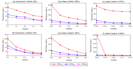
Figure 3. Runtime under various parameters (minfre, minpro and period).

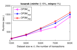
Figure 4. Scalability test.

Furthermore, we performed an experiment to asses the scalability of OP3M w.r.t the number of transactions. We ran the proposed profit-based OP3M model on kosarak dataset with minfre: 0.15% and minpro: 1%, and varied the number of transactions from 100,000 to 900,000. Results of scalability test are shown in Fig. 4. In general, runtime is an estimate of how long it takes to perform such an analysis. Form the results, it can be observed that OP3M has linear scalability w.r.t the number of transactions.

6. Conclusion

In this paper, we have presented a novel framework named OP3M for searching on-shelf popular and most profitable products in databases where both positive and negative profit values appeared and on-shelf time of products are considered. This is the first work to systematically study the problem of profit-based optimization for Economic behavior, including purchase frequency, on-shelf availability w.r.t. purchase time periodic, and profit. Given some historical datasets on market share, the designed algorithm can help us to make sense of the users’ economic behavior and find the on-shelf popular and most profitable products. OP3M also brings several improvements over existing technologies. Based on the developed profit-based OPP-lists, it is a single phase algorithm that does not need to maintain candidates in memory. It relies on the novel concept named remaining positive profit, and uses a depth-first search rather than a level-wise search. Moreover, OP3M finds OPPPs in all time periods at the same time rather than separately searching each period and performing costly intersection operations of the results of each time period. The extensive performance evaluation on several datasets demonstrates the effectiveness and efficiency of the OP3M algorithm.

References

- (1)
- Agrawal et al. (1994) Rakesh Agrawal, Ramakrishnan Srikant, et al. 1994. Fast algorithms for mining association rules. In Proceedings of the 20th International Conference on Very Large Data Bases. 487–499.
- Ahmed et al. (2009) Chowdhury-Farhan Ahmed, Syed Khairuzzaman Tanbeer, Byeong-Soo Jeong, and Young-Koo Lee. 2009. Efficient tree structures for high utility pattern mining in incremental databases. IEEE Transactions on Knowledge and Data Engineering 21, 12 (2009), 1708–1721.
- Coleman and Fararo (1992) James S Coleman and Thomas J Fararo. 1992. Rational choice theory. Nueva York: Sage (1992).
- Corsten and Gruen (2003) Daniel Corsten and Thomas Gruen. 2003. Desperately seeking shelf availability: an examination of the extent, the causes, and the efforts to address retail out-of-stocks. International Journal of Retail & Distribution Management 31, 12 (2003), 605–617.
- Duong et al. (2016) Quang-Huy Duong, Bo Liao, Philippe Fournier-Viger, and Thu Lan Dam. 2016. An efficient algorithm for mining the top-k high utility itemsets, using novel threshold raising and pruning strategies. Knowledge-Based Systems 104 (2016), 106–122.
- Fournier-Viger et al. (2017) Philippe Fournier-Viger, Jerry Chun-Wei Lin, Rage Uday Kiran, Yun-Sing Koh, and Rincy Thomas. 2017. A survey of sequential pattern mining. Data Science and Pattern Recognition 1, 1 (2017), 54–77.
- Fournier-Viger and Zida (2015) Philippe Fournier-Viger and Souleymane Zida. 2015. FOSHU: faster on-shelf high utility itemset mining–with or without negative unit profit. In The 30th Annual ACM Symposium on Applied Computing. 857–864.
- Gan et al. (2021) Wensheng Gan, Chun Wei Lin, Philippe Fournier-Viger, Han Chieh Chao, Vincent Tseng, and Philip S Yu. 2021. A survey of utility-oriented pattern mining. IEEE Transactions on Knowledge and Data Engineering 33, 4 (2021), 1306–1327.
- Gan et al. (2018a) Wensheng Gan, Jerry Chun-Wei Lin, Han-Chieh Chao, Shyue-Liang Wang, and Philip S Yu. 2018a. Privacy preserving utility mining: a survey. In Proceedings of the IEEE International Conference on Big Data. IEEE, 2617–2626.
- Gan et al. (2018b) Wensheng Gan, Jerry Chun-Wei Lin, Philippe Fournier-Viger, Han-Chieh Chao, Tzung-Pei Hong, and Hamido Fujita. 2018b. A survey of incremental high-utility itemset mining. Wiley Interdisciplinary Reviews: Data Mining and Knowledge Discovery 8, 2 (2018).
- Ge et al. (2015) Shen Ge, Nikos Mamoulis, David WL Cheung, et al. 2015. Dominance relationship analysis with budget constraints. Knowledge and Information Systems 42, 2 (2015), 409–440.
- Geng and Hamilton (2006) Liqiang Geng and Howard J Hamilton. 2006. Interestingness measures for data mining: A survey. Comput. Surveys 38, 3 (2006), 9.
- Guns et al. (2011a) Tias Guns, Siegfried Nijssen, and Luc De Raedt. 2011a. Itemset mining: A constraint programming perspective. Artificial Intelligence 175, 12-13 (2011), 1951–1983.
- Guns et al. (2011b) Tias Guns, Siegfried Nijssen, and Luc De Raedt. 2011b. k-Pattern set mining under constraints. IEEE Transactions on Knowledge and Data Engineering 25, 2 (2011), 402–418.
- Guns et al. (2011c) Tias Guns, Siegfried Nijssen, Albrecht Zimmermann, and Luc De Raedt. 2011c. Declarative heuristic search for pattern set mining. In IEEE 11th International Conference on Data Mining Workshops. IEEE, 1104–1111.
- Han et al. (2004) Jiawei Han, Jian Pei, Yiwen Yin, and Runying Mao. 2004. Mining frequent patterns without candidate generation: A frequent-pattern tree approach. Data Mining and Knowledge Discovery 8, 1 (2004), 53–87.
- Koh and Ravana (2016) Yun-Sing Koh and Sri-Devi Ravana. 2016. Unsupervised rare pattern mining: a survey. ACM Transactions on Knowledge Discovery from Data 10, 4 (2016), 45.
- Lan et al. (2015) Guo-Cheng Lan, Tzung-Pei Hong, Yi-Hsin Lin, and Shyue-Liang Wang. 2015. Fuzzy utility mining with upper-bound measure. Applied Soft Computing 30 (2015), 767–777.
- Lan et al. (2014) Guo-Cheng Lan, Tzung-Pei Hong, Vincent S Tseng, and Shyue-Liang Wang. 2014. Applying the maximum utility measure in high utility sequential pattern mining. Expert Systems with Applications 41, 11 (2014), 5071–5081.
- Li et al. (2011) Beibei Li, Anindya Ghose, and Panagiotis G Ipeirotis. 2011. Towards a theory model for product search. In Proceedings of the 20th International Conference on World Wide Web. ACM, 327–336.
- Lin et al. (2016a) Jerry Chun-Wei Lin, Philippe Fournier-Viger, and Wensheng Gan. 2016a. FHN: An efficient algorithm for mining high-utility itemsets with negative unit profits. Knowledge-Based Systems 111 (2016), 283–298.
- Lin et al. (2016c) Jerry Chun-Wei Lin, Wensheng Gan, Philippe Fournier-Viger, Tzung-Pei Hong, and Vincent S Tseng. 2016c. Efficient algorithms for mining high-utility itemsets in uncertain databases. Knowledge-Based Systems 96 (2016), 171–187.
- Lin et al. (2016d) Jerry Chun-Wei Lin, Wensheng Gan, Philippe Fournier-Viger, Tzung-Pei Hong, and Vincent S Tseng. 2016d. Fast algorithms for mining high-utility itemsets with various discount strategies. Advanced Engineering Informatics 30, 2 (2016), 109–126.
- Lin et al. (2017) Jerry Chun-Wei Lin, Wensheng Gan, Philippe Fournier-Viger, Tzung-Pei Hong, and Vincent S Tseng. 2017. Efficiently mining uncertain high-utility itemsets. Soft Computing 21, 11 (2017), 2801–2820.
- Lin et al. (2016b) Jerry Chun-Wei Lin, Wensheng Gan, and Tzung-Pei Hong. 2016b. A fast maintenance algorithm of the discovered high-utility itemsets with transaction deletion. Intelligent Data Analysis 20, 4 (2016), 891–913.
- Lin et al. (2015a) Jerry Chun-Wei Lin, Wensheng Gan, Tzung-Pei Hong, and Vincent S Tseng. 2015a. Efficient algorithms for mining up-to-date high-utility patterns. Advanced Engineering Informatics 29, 3 (2015), 648–661.
- Lin et al. (2015b) Jerry Chun-Wei Lin, Wensheng Gan, Tzung-Pei Hong, and Binbin Zhang. 2015b. An incremental high-utility mining algorithm with transaction insertion. The Scientific World Journal 2015 (2015).
- Lin et al. (2015c) Yu-Feng Lin, Cheng-Wei Wu, Chien-Feng Huang, and Vincent S Tseng. 2015c. Discovering utility-based episode rules in complex event sequences. Expert Systems with Applications 42, 12 (2015), 5303–5314.
- Liu et al. (2005) Ying Liu, Wei-keng Liao, and Alok Choudhary. 2005. A two-phase algorithm for fast discovery of high utility itemsets. In Pacific-Asia Conference on Knowledge Discovery and Data Mining. Springer, 689–695.
- Mai et al. (2017) Thang Mai, Bay Vo, and Loan TT Nguyen. 2017. A lattice-based approach for mining high utility association rules. Information Sciences 399 (2017), 81–97.
- Marshall (2005) Alfred Marshall. 2005. From Principles of Economics. In Readings in the Economics of the Division of Labor: the Classical Tradition. World Scientific, 195–215.
- Marshall (2009) Alfred Marshall. 2009. Principles of economics: unabridged eighth edition. Cosimo, Inc.
- Nguyen et al. (2019) Loan TT Nguyen, Phuc Nguyen, Trinh DD Nguyen, Bay Vo, Philippe Fournier-Viger, and Vincent S Tseng. 2019. Mining high-utility itemsets in dynamic profit databases. Knowledge-Based Systems (2019).
- Peng et al. (2012) Yu Peng, Raymond Chi-Wing Wong, and Qian Wan. 2012. Finding top-k preferable products. IEEE Transactions on Knowledge and Data Engineering 24, 10 (2012), 1774–1788.
- Quattrone et al. (2016) Giovanni Quattrone, Davide Proserpio, Daniele Quercia, Licia Capra, and Mirco Musolesi. 2016. Who benefits from the sharing economy of Airbnb?. In Proceedings of the 25th International Conference on World Wide Web. ACM, 1385–1394.
- Rymon (1992) Ron Rymon. 1992. Search through systematic set enumeration. Proceeding of the 3rd International Conference on Principles of Knowledge Representation and Reasoning (1992), 539–550.
- Teng et al. (2015) Ya-Wen Teng, Chih-Hua Tai, Philip S Yu, and Ming-Syan Chen. 2015. An effective marketing strategy for revenue maximization with a quantity constraint. In Proceedings of the 21th ACM SIGKDD International Conference on Knowledge Discovery and Data Mining. ACM, 1175–1184.
- Tseng et al. (2013) Vincent S Tseng, Bai-En Shie, Cheng-Wei Wu, and Philip S Yu. 2013. Efficient algorithms for mining high utility itemsets from transactional databases. IEEE Transactions on Knowledge and Data Engineering 25, 8 (2013), 1772–1786.
- Tseng et al. (2016) Vincent S Tseng, Cheng-Wei Wu, Philippe Fournier-Viger, and Philip S Yu. 2016. Efficient algorithms for mining top- high utility itemsets. IEEE Transactions on Knowledge and Data Engineering 28, 1 (2016), 54–67.
- Ugarte et al. (2017) Willy Ugarte, Patrice Boizumault, Bruno Crémilleux, Alban Lepailleur, Samir Loudni, Marc Plantevit, Chedy Raïssi, and Arnaud Soulet. 2017. Skypattern mining: From pattern condensed representations to dynamic constraint satisfaction problems. Artificial Intelligence 244 (2017), 48–69.
- Wang and Zhang (2011) Jian Wang and Yi Zhang. 2011. Utilizing marginal net utility for recommendation in e-commerce. In Proceedings of the 34th International ACM SIGIR Conference on Research and Development in Information Retrieval. ACM, 1003–1012.
- Wang and Huang (2018) Jun-Zhe Wang and Jiun-Long Huang. 2018. On Incremental High Utility Sequential Pattern Mining. ACM Transactions on Intelligent Systems and Technology 9, 5 (2018), 55.
- Wu et al. (2013) Cheng-Wei Wu, Yu-Feng Lin, Philip S Yu, and Vincent S Tseng. 2013. Mining high utility episodes in complex event sequences. In Proceedings of the 19th ACM SIGKDD International Conference on Knowledge Discovery and Data Mining. ACM, 536–544.
- Xu and Lui (2016) Silei Xu and John Lui. 2016. Product selection problem: improve market share by learning consumer behavior. ACM Transactions on Knowledge Discovery from Data 10, 4 (2016), 34.
- Yang et al. (2016) Jianye Yang, Ying Zhang, Wenjie Zhang, and Xuemin Lin. 2016. Influence based cost optimization on user preference. In Proceedings of the IEEE 32nd International Conference on Data Engineering. IEEE, 709–720.
- Yang et al. (2007) Zhenglu Yang, Lin Li, Botao Wang, and Masaru Kitsuregawa. 2007. Towards efficient dominant relationship exploration of the product items on the web. In Proceedings of the 16th International Conference on World Wide Web. ACM, 1205–1206.
- Yin et al. (2012) Junfu Yin, Zhigang Zheng, and Longbing Cao. 2012. USpan: an efficient algorithm for mining high utility sequential patterns. In Proceedings of the 18th ACM SIGKDD International Conference on Knowledge Discovery and Data Mining. ACM, 660–668.
- Yin et al. (2013) Junfu Yin, Zhigang Zheng, Longbing Cao, Yin Song, and Wei Wei. 2013. Efficiently mining top- high utility sequential patterns. In Proceedings of the IEEE 13th International Conference on Data Mining. IEEE, 1259–1264.
- Ying et al. (2014) Jia-Ching Ying, Huan-Sheng Chen, Kawuu W Lin, Eric Hsueh-Chan Lu, Vincent S Tseng, Huan-Wen Tsai, Kuang Hung Cheng, and Shun-Chieh Lin. 2014. Semantic trajectory-based high utility item recommendation system. Expert Systems with Applications 41, 10 (2014), 4762–4776.
- Zhang and Chen (2018) Yongfeng Zhang and Xu Chen. 2018. Explainable recommendation: A survey and new perspectives. arXiv preprint arXiv:1804.11192 (2018).
- Zhang et al. (2016) Yongfeng Zhang, Qi Zhao, Yi Zhang, Daniel Friedman, Min Zhang, Yiqun Liu, and Shaoping Ma. 2016. Economic recommendation with surplus maximization. In Proceedings of the 25th International Conference on World Wide Web. ACM, 73–83.
- Zhao et al. (2012) Gang Zhao, Mong Li Lee, Wynne Hsu, and Wei Chen. 2012. Increasing temporal diversity with purchase intervals. In Proceedings of the 35th International ACM SIGIR Conference on Research and Development in Information Retrieval. ACM, 165–174.
- Zhao et al. (2017) Qi Zhao, Yongfeng Zhang, Yi Zhang, and Daniel Friedman. 2017. Multi-product utility maximization for economic recommendation. In Proceedings of the Tenth ACM International Conference on Web Search and Data Mining. ACM, 435–443.