Iterative Genetic Improvement: Scaling Stochastic Program Synthesis

Abstract

Program synthesis aims to automatically find programs from an underlying programming language that satisfy a given specification. While this has the potential to revolutionize computing, how to search over the vast space of programs efficiently is an unsolved challenge in program synthesis. In cases where large programs are required for a solution, it is generally believed that stochastic search has advantages over other classes of search techniques. Unfortunately, existing stochastic program synthesizers do not meet this expectation very well, suffering from the scalability issue. Here we propose a new framework for stochastic program synthesis, called iterative genetic improvement to overcome this problem, a technique inspired by the practice of the software development process. The key idea of iterative genetic improvement is to apply genetic improvement to improve a current reference program, and then iteratively replace the reference program by the best program found. Compared to traditional stochastic synthesis approaches, iterative genetic improvement can build up the complexity of programs incrementally in a more robust way. We evaluate the approach on two program synthesis domains: list manipulation and string transformation. Our empirical results indicate that this method has considerable advantages over several representative stochastic program synthesizer techniques, both in terms of scalability and of solution quality.

I INTRODUCTION

Program synthesis is a longstanding challenge in artificial intelligence (AI) and has even been considered by some as the ”holy grail of computer science” gulwani2017program . The goal of program synthesis is to automatically write a program that has a behavior consistent with a specification. The specification itself can be expressed in various forms such as logical specification manna1980deductive ; srivastava2010program , examples bauer1979programming ; gulwani2011automating ; gulwani2016programming ; balog2017deepcoder or in natural language descriptions desai2016program ; yaghmazadeh2017sqlizer ; shin2019program . Program synthesis techniques have been used successfully in many real-world application domains including data wrangling gulwani2011automating ; devlin2017robustfill ; chen2021spreadsheetcoder , program repair le2012systematic ; yuan2020arja , computer graphics gulwani2011synthesizing ; ellis2018learning and others. Furthermore, viewing machine learning tasks as program synthesis ellis2015unsupervised ; trivedi2021learning can potentially address some of the difficulties of modern deep learning approaches, e.g., data hunger or poor interpretability, leading to more reliable and interpretable AI.

Recently, program synthesis has seen a renaissance in several different research communities, particularly in the programming language and the machine learning community. Most research efforts focus on developing more effective search techniques since program synthesis is a notoriously difficult combinatorial search problem. Enumerative search-based synthesis alur2018search enumerates programs in the search space according to a specific order, a topic well studied in the literature. But this class of techniques is usually inefficient and needs to be augmented with strategies (i) to prune the search space gulwani2011automating ; alur2017scaling , (ii) to bias the search using probabilistic models balog2017deepcoder ; lee2018accelerating ; odena2021bustle , or (iii) to split a large problem via divide-and-conquer strategies alur2017scaling ; huang2020reconciling . Despite such augmentations, enumerative search still struggles to scale to large program sizes, as the search space grows exponentially with program size. Another popular class of search techniques is to reduce the program synthesis problem by constraint solving, and leverage off-the-shelf SAT/SMT solvers to efficiently explore the search space solar2008program ; jha2010oracle ; feng2018program . Although this class of techniques has achieved impressive results alur2019syguscomp , it also has difficulty in synthesizing large programs due to the limited power of the underlying SAT/SMT solvers.

Stochastic program synthesis (SPS) employs stochastic search methods such as the Metropolis-Hastings (MH) algorithm chib1995understanding or genetic programming (GP) koza1992genetic ; banzhaf1998genetic in order to explore the space of programs. Compared to the above mentioned search techniques, SPS is a very promising technique for addressing harder synthesis problems that require larger programs gulwani2016technical . However, this potential of SPS is currently far from being fully exploited. According to the experiments done in alur2013syntax , a typical MH approach for program synthesis has been shown to be not very effective compared to other approaches. One possible drawback of the MH approach is that it cannot make the corresponding local changes when a program is close to being correct, because the proposal distribution used can only lead to big changes in a program sps2018 .

The Genetic Programming (GP) method was always intended for automatic programming, but has suffered from scalability issues for quite a long time o2019automatic . For hard problems, GP can be very slow and the well-known continued growth of programs without fitness improvement (’bloat’) greatly limits its applicability gustafson2004problem . Although there have been some methods to handle code growth luke2006comparison , they usually result in unsatisfactory or even worse performance gustafson2004problem ; luke2006comparison . Besides MH and GP, stochastic local search (SLS) hoos2004stochastic , such as simulated annealing, would be another alternative, but it has received little attention o1995analysis in program synthesis. One serious limitation of SLS is that it can easily get trapped in local minima, given that the search space of programs is often highly rugged and contains many plateaus schulte2014software ; langdon2017software .

In this paper, we propose an iterative genetic improvement (IGI) method to make SPS more scalable for finding large programs as solutions. Our approach is inspired by a practical software development technique called iterative enhancement basil1975iterative , where human programmers write a simple initial implementation and then enhance it iteratively until a final implementation is achieved. Based on this paradigm, our basic idea is to consider a sequence of program improvements just like the evolution from a primitive cell to a sophisticated and specialized cell banzhaf2018some . Our proposed IGI starts with a random program, then the current program is improved iteratively by applying genetic improvement (GI) petke2018genetic which evolves modifications to the current program. When no improvements can be made any more by GI, a perturbation operator is applied that will allow to continue the iterative improvement process. Because IGI carefully rewrites small parts of a current program via GI in each iteration, it can largely avoid unnecessarily big code changes like those of the MH approach alur2013syntax , or the code growth problem GP faces, leading to faster search. Moreover, IGI considers a neighborhood of the current program that is much larger than SLS based techniques such as SA o1995analysis , so it is more able to avoid or escape local minima and plateaus. We demonstrate the superiority of IGI on two different program synthesis domains and compare with several representative SPS techniques. Our experimental results show that IGI can outperform all of the compared techniques by a large margin in terms of scalability. In addition, our results also indicate that IGI appears to be less prone to overfitting.

The rest of this paper is organized as follows. In Section II we discuss some background material for our study. Section III describes the proposed IGI method in detail. Section IV presents empirical results while Section V briefly introduces other work related to this study. Section VI summarizes and concludes.

II Preliminaries and Background

II.1 Domain-Specific Language

A domain-specific language (DSL) is a computer language that is specifically created for a particular domain. Program synthesis is usually based on a given DSL in order to take a first cut at the space of possible programs.

A DSL can be expressed as a primitive set which includes functions and terminals assumed to be useful for solving problems in a specific domain. Consider a toy DSL with the primitive set $\{\texttt{ADD},\texttt{SUB},\texttt{EQ},\texttt{ITE},0,1,\text{IN0},\text{IN1}\}$. In this primitive set, ADD, SUB, EQ and ITE are functions explained in Table 1, and the remaining four entities are terminals. Among the four terminals, integers 0 and 1 are constants, and integers IN0 and IN1 are external inputs to the program.

Table 1: Description of functions in the DSL.

Symbol	Arguments	Return Type	Description
ADD	$x,y$: Integer	Integer	Return $x+y$.
SUB	$x,y$: Integer	Integer	Return $x-y$.
EQ	$x,y$: Integer	Boolean	If $x$ is equal to $y$, return true,
			otherwise return false.
ITE	$c$: Boolean;	Integer	If $c$ is true, return $x$,
	$x,y$: Integer		otherwise return $y$.

The primitive set of a DSL defines the complete hypothesis space of possible programs. Each program can be represented as an expression tree. Figure 1 shows such a tree for a valid program in the above toy DSL.

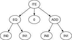
Figure 1: The tree of the valid program ITE(EQ(IN0, IN1), 0, ADD(IN0, IN1)) in the above toy DSL.

In our experiments, we will consider two DSLs. One is useful for list manipulation (referred to as DSL-LM), and the other is useful for string transformation (referred to as DSL-ST). They are described in detail in Appendix A and Appendix B, respectively.

II.2 Programming by Example

Programming by example (PBE) is a subfield of program synthesis, where the specification is given in the form of input-output (IO) examples.

Assume that we have a DSL that defines the space of all possible programs denoted by $\mathcal{P}$. In PBE, a task is described by a set of IO examples $\mathcal{X}=\{(I_{1},O_{1}),\ldots,(I_{n},O_{n})\}$. We can then say we have solved this task if we find a program $\mathbf{p}\in\mathcal{P}$ that can map correctly every input in $\mathcal{X}$ to the corresponding output, i.e., $\mathbf{p}(I_{i})=O_{i},\forall i=1,2,\ldots,n$. Table 2 shows a PBE task with four IO examples and a potential correct program from the toy DSL described in Section II.1.

Table 2: A PBE task with four IO examples (each input contains two integers) and a possible program in the toy DSL that satisfies all of the four examples.

Input ($I_{i}$)	Output ($O_{i}$)	Program
3, 3	0	ITE(EQ(IN0, IN1), 0, ADD(IN0, IN1))
2, 5	7
8, 1	9
6, 6	0

Our goal is to build a program synthesizer which can find such a program $\mathbf{p}$ in $\mathcal{P}$ according to the IO specification $\mathcal{X}$ within a certain time limit.

II.3 Genetic Improvement

Genetic improvement (GI) petke2018genetic is the use of an automated search algorithm, genetic programming, to improve an existing program. GI typically conducts the search over the space of patches, where a patch constitutes a sequence of edits that are applied to the original program and corresponds to a modified program. Compared to the original program, an improved version needs to have better functional properties (e.g., by eliminating buggy behavior) le2012systematic ; yuan2020arja ; yuan2020toward or better non-functional properties (e.g., shorter execution time or smaller energy consumption) langdon2015optimizing ; bruce2015reducing , depending on the application scenario or an user’s goal. GI has achieved notable success in software repair and optimization. For example, a GI approach langdon2015optimizing can find code that is 70 times faster (on average), when applied to a widely-used DNA sequencing system called Bowtie2.

In this paper, GI improves a program with respect to a fitness function measuring how well the program performs over a given set of input-output examples.

III Iterative Genetic Improvement

III.1 Overview

The IGI framework proposed here is described in Algorithm 1. First, in Step 1, we create $K$ program trees randomly using ramped half-and-half initialization koza1992genetic with a depth range of $[d_{\min},d_{\max}]$. The best among these $K$ random programs is set to become the initial program $\mathbf{p}_{0}$. This step is intended to find a good starting point for the search by sampling from a (substantial) number of programs instead of a single one.

Algorithm 1 Framework of the Proposed IGI

1.  $\mathbf{p}_{0}\leftarrow\texttt{InitProg}(d_{\min},d_{\max},K)$

2.  $\mathbf{p}\leftarrow\texttt{IterGenImprov}(\mathbf{p}_{0})$

3.  while termination criterion is not satisfied do

4.     $\mathbf{p}^{\prime}\leftarrow\texttt{Perturbation}(\mathbf{p}$)

5.     $\mathbf{p}^{\prime\prime}\leftarrow\texttt{IterGenImprov}(\mathbf{p}^{\prime})$

6.     $\mathbf{p}\leftarrow\texttt{AcceptanceCriterion}(\mathbf{p},\mathbf{p}^{\prime\prime})$

7.  end while

8.  return  the best program found

In Step 2, we make incremental improvements from $\mathbf{p}_{0}$ by applying the GI procedure iteratively until a program $\mathbf{p}$ is reached that cannot be further improved by the adopted GI. In each iteration GI tries to produce an improved version $p_{i+1}$ by searching for modifications to the current program $p_{i}$. Figure 2 illustrates this process where $\mathbf{p}_{l}=\mathbf{p}$, and we call the process from $\mathbf{p}_{i}$ to $\mathbf{p}_{i+1}$ an epoch, where $\mathbf{p}_{i+1}$ is an improved version of $\mathbf{p}_{i}$ obtained through GI.

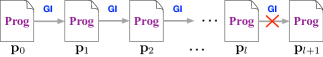
Figure 2: Illustration of Step 2 in Algorithm 1. $\mathbf{p}_{i+1}$ is an improved version of $\mathbf{p}_{i}$ for $i=0,1,\ldots,l-1$, that is obtained by applying GI to $\mathbf{p}_{i}$. Since $\mathbf{p}_{l+1}$ is not better than $\mathbf{p}_{l}$ (i.e., GI fails to improve $\mathbf{p}_{l}$), $\mathbf{p}_{l}$ is finally returned by IterGenImprov.

After Step 2, to continue the search, we need to generate a new starting program for IterGenImprov. To do this, a naive strategy is to randomly produce a new program as the starting program. However this strategy is obviously not efficient because the search history is completely discarded. Here we follow the basic idea of iterated local search lourencco2019iterated . That is, we apply some perturbation operator to $\mathbf{p}$ that leads to an intermediate program $\mathbf{p}^{\prime}$ (Step 4 in Algorithm 1). Then IterGenImprov restarts the search from $\mathbf{p}^{\prime}$ and returns $\mathbf{p}^{\prime\prime}$ (Step 5 in Algorithm 1). In Step 6, AcceptanceCriterion will decide to which program the next time Perturbation is applied. In this paper, this criterion just simply returns the better of $\mathbf{p}$ and $\mathbf{p}^{\prime\prime}$. Steps 4–6 are iterated until some termination criterion is met.

As can be seen in IGI, we need to compare the quality of two programs frequently. This is aided by a predefined fitness function which can measure how well a program satisfies the given specification. Suppose we are given a set of $n$ input-output examples $\{(I_{1},O_{1}),\ldots,(I_{n},O_{n})\}$, the fitness function of a program $\mathbf{p}$ can be defined as $fitness(\mathbf{p})=\frac{1}{n}\sum_{i=1}^{n}sim(O_{i},\mathbf{p}(I_{i}))$, where $sim$ function indicates the similarity between the expected output $O_{i}$ and the actual output $\mathbf{p}(I_{i})$. In our study, for DSL-LM, $sim$ returns 1 if $O_{i}=\mathbf{p}(I_{i})$ otherwise returns 0. As for DSL-ST, we use a finer-grained $sim$ function which returns the normalized Levenshtein similarity between two strings. In our approach, a program with larger fitness is better, while in the case of two programs having the same fitness, the program with smaller size is deemed better according to Occam’s razor. A program $\mathbf{p}$ will satisfy the given specification iff it achieves maximum fitness (i.e., $fitness(\mathbf{p})=1$).

Section III.2 will detail how to apply GI to the current program $\mathbf{p}_{i}$ to get an improved version $\mathbf{p}_{i+1}$, which corresponds to one epoch in IterGenImprov (see Figure 2). Section III.3 will explain how to conduct the perturbation operator, which corresponds to Step 4 in Algorithm 1.

III.2 Applying Genetic Improvement

III.2.1 Patch Representation

A program different from the program we want to improve can be coded as the difference between the original and the new program. In computing, this is known as a program patch, represented as a sequence of edits to the program’s expression tree. In this patch representation, we define three kinds of edits: replacement, insertion and deletion. Syntactic and type constraints are considered in these edits in order to ensure that the modified tree remains legal. To randomly generate an edit, we first select a node randomly in the expression tree that is called target node. Then we choose one of the three kinds of edits randomly.

1) Replacement: If we choose to perform replacement, the target node is replaced by another random primitive from the primitive set which has the same number of arguments, the same argument types and the same return type. This is illustrated in Figure 3.

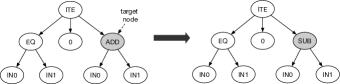
Figure 3: Illustration of a replacement edit (shaded nodes are changed).

2) Insertion: If we choose to perform insertion, for the primitive that can be inserted, its return type and at least one of its argument types should be the same as the return type of the target node. Such a primitive is selected at random from the primitive set. Then this primitive will replace the target node, and the subtree rooted at the target node will become one of its child tree that requires the same data type. All the remaining children of this primitive will be selected randomly from the set of terminals with the corresponding data types. This is illustrated in Figure 4.

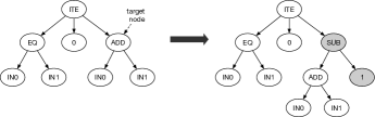
Figure 4: Illustration of an insertion edit (shaded nodes are the newly inserted nodes).

3) Deletion: If we choose to perform deletion, one node is randomly chosen from the children of the target node that have the same return type as the target node. The subtree rooted at this node will replace the subtree rooted at the target node. This is illustrated in Figure 5.

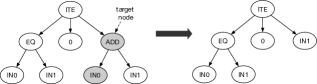
Figure 5: Illustration of a deletion edit (shaded nodes are removed from the original tree).

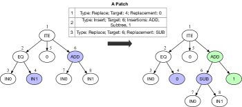
Figure 6: Illustration of a patch that contains three edits. The number above the node is the ID of the node. The blue shaded nodes are changed by replacement edits and the green shaded nodes are the new nodes added by the insertion edit.

A patch contains a list of concrete edits and each edit is performed sequentially when applying the patch. This is illustrated in Figure 6.

In our study, we find that the above replacement/insertion edits sometimes struggle to introduce the following two kinds of primitives into the program. First, if the return type of a primitive is different from all its argument types (e.g., the primitive LEN in the DSL-ST), we know that it is hard or even impossible to bring the two kinds of primitives using the above insertion edit. Second, if there are no corresponding terminals for some of its argument types of a primitive (e.g., the primitive Take in the DSL-LM), the situation is similar. Also, a replacement edit might have little chance to get introduced into a program, if there are few (or even no) primitives with the same return type and argument types in the set. Should the desired program really require this primitive, the search will become inefficient. We address the generation of replacement and insertion edits to introduce the two kinds of primitives easily as follows:
For the replacement edit, when the target node is a leaf, a function with the same return type is also allowed to replace the target node and the arguments of this function will be filled with random terminals having the corresponding types. This is demonstrated in Figure 7.

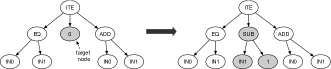
Figure 7: Illustration of a replacement edit (shaded node in the original tree is replaced by the shaded nodes in the new tree).

As for the insertion edit, when the algorithm fails to find a terminal for a child of the inserted node, it instead chooses a function with the desired return type and fill its arguments with random terminals having the corresponding types. This is demonstrated in Figure 8.

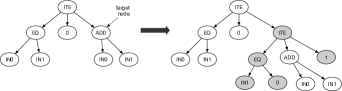
Figure 8: Illustration of an insertion edit (shaded node are the newly inserted nodes).

Note that there may exist conflicts between two edits. For example, a replacement edit as shown in Figure 3 and a deletion edit as shown in Figure 5 cannot take effect at the same time. We resolve such conflicts at the time of generating or applying a patch by disabling the latter one if it conflicts with a previous edit.

Using this patch representation, we can search for patches to the current program $\mathbf{p}_{i}$ that are able to produce an improved version $\mathbf{p}_{i+1}$. In our framework, we provide two alternative search algorithms: stochastic beam search (SBS) and linear genetic programming (LGP) brameier2007linear , which are described in the next subsections III.2.2 and III.2.3, respectively.

III.2.2 Stochastic Beam Search

In stochastic beam search (SBS), the search for patches of length $L+1$ is based on the patches of length $L$ (i.e., there are already $L$ edits in the patch). Suppose that we currently have a set of $B$ patches of length $L$. Then for each of the $B$ patches, we produce $C$ copies and append a randomly generated edit to each copy where the appended edit should not conflict with the previous $L$ edits. Having produced a total of $B\times C$ patches of length $L+1$, tournament selection is used to select $B$ patches from the total $B\times C$. Based on these $B$ patches of length $L+1$, SBS continues to explore further patches, this time of length $L+2$.

SBS starts the search from $B$ empty patches (i.e., length $L=0$), with a limiting parameter $L_{\max}$ used to restrict the maximum length of allowed patches. Once SBS finds a program $\mathbf{p}_{i}^{\prime}$ that is better than the current program $\mathbf{p}_{i}$, we need to decide whether to continue SBS or just return $\mathbf{p}_{i}^{\prime}$ as $\mathbf{p}_{i+1}$ for the next GI epoch. In this study, our strategy is that if $\mathbf{p}_{i}^{\prime}$ is the best program ever found from the beginning of IGI, SBS in this GI epoch is deemed to be fruitful and continues searching for better return programs until it reaches $L_{\max}$. Otherwise $\mathbf{p}_{i}^{\prime}$ can be simply returned as $\mathbf{p}_{i+1}$. Note that SBS may fail to find any improved version of the current program $\mathbf{p}_{i}$ after reaching $L_{\max}$, in this case the perturbation operator will be invoked.

III.2.3 Linear Genetic Programming

In the linear genetic programming (LGP) approach, the search starts with a population of $N$ random patches denoted $\mathcal{P}_{0}$. To produce patches with diverse lengths, each patch length in $\mathcal{P}_{0}$ is drawn from a $1+Poisson(1)$ distribution, where $Poisson(\lambda)$ is a Poisson distribution with parameter $\lambda=1$.

In the $g$-th generation of LGP, we use tournament selection to select two parent patches from $\mathcal{P}_{g}$ and apply crossover and mutation to the two patches to generate two offspring. By repeating this process $N/2$ times, $N$ offspring patches are generated which constitute the next population $\mathcal{P}_{g+1}$.

One-point crossover between two parent patches is used. Suppose that the length of the two parents is $L_{1}$ and $L_{2}$, respectively. We use a cut point in the two parents given by $\lfloor\alpha L_{1}\rfloor$ and $\lfloor\alpha L_{2}\rfloor$, where $\alpha\in(0,1)$ is a random value. The edits after the cut points are swapped between the two parent patches, leading to two offspring.

Mutation is then applied to each of the two offspring patches. When applying mutation to a patch, an edit in the patch is selected uniformly at random, and with equal probabilities removed, replaced with a random edit, or a random edit is inserted after the selected one.

In LGP, we use the same strategy as in SBS to determine when to terminate the search and return the best program LGP has found during the current epoch of GI.

III.3 Perturbation Operator

The goal of the perturbation operator is to provide a new good starting program for the next application of IterGenImprov in case we get stuck.

When applying the perturbation to $\mathbf{p}$ (Step 4 in Algorithm 1), some useful components of $\mathbf{p}$ need to be conserved, in order to provide a new good starting program for the next application of IterGenImprov. At the same time the perturbation should not be too small, in order to avoid staying stuck in the same local optimum as the previous epoch of IterGenImprov.

In our framework, the perturbation operator works as follows: First, we collect a set of nodes denoted by $\mathcal{N}$ from the expression tree of $\mathbf{p}$, where the size of the subtree rooted at each node is not smaller than $S_{\min}$. Second, we randomly select a node $\nu$ from $\mathcal{N}$. For convenience, the subtree rooted at node $\nu$ is denoted by $\mathcal{T}$ and its size is denoted by $S_{\mathcal{T}}$. Third, we randomly generate $M$ trees with size in the range $[1,S_{\mathcal{T}}]$ and the same return type as $\mathcal{T}$. Fourth, we replace $\mathcal{T}$ in the tree of $\mathbf{p}$ with each of the $M$ trees in turn, and obtain $M$ new programs. Last, the best program among the $M$ programs is returned as the perturbed program $\mathbf{p}^{\prime}$.

In addition, we handle two special cases: One is that $\mathcal{N}=\emptyset$ and the other is that the selected node $\nu$ is the root node. For both of these cases, we invoke the initialization function InitProg to produce a program that is used as the perturbed program $\mathbf{p}^{\prime}$.

As can be seen from above, $S_{\min}$ is the parameter that restricts the minimum strength of a perturbation. Since we know that a random subtree replacement usually leads to a bad fitness of the new program in program synthesis, our perturbation operator generates $M$ candidate program variants instead of a single one. Moreover, with a relatively low probability, the perturbation operator can ignore much (when $\nu$ is the node very close to root) or even all (when $\nu$ is the root node) of the information of $\mathbf{p}$, which can help to explore other promising regions of the program space.

IV Experiments

IV.1 Experimental Setup

The IGI framework is instantiated here with SBS (see Section III.2.2) and LGP (see Section III.2.3), resulting in two algorithms IGI-SBS and IGI-LGP, respectively. The source code is implemented in Python and has been made available at GitHub. All the experiments are conducted on the Intel Xeon E5-2680 2.4GHz CPU processor with 20GB memory.

IV.1.1 Benchmarks

We evaluate the algorithms on synthesis tasks from two different application domains: list manipulation and string transformation. The corresponding DSLs for the two domains are described in Appendix A and B.

For the list manipulation domain, 200 benchmarks are generated, similar to balog2017deepcoder . In particular, we first randomly generate a program with a number of tree nodes in the range between 10 and 15. Then we generate random input/output pairs for this program. This process is repeated until we either obtain 100 valid input-output examples or no examples can be found within a fixed iteration limit, in which case we discard it and start over again. Note that in order to test the scalability of SPS techniques, we consider larger oracle programs than existing studies balog2017deepcoder ; feng2018program ; chen2020program . For example, oracle programs with at most seven nodes were investigated in balog2017deepcoder .

As for the second domain, string transformations, we use the dataset consisting of all SyGuS tasks whose outputs are only strings from the PBE-Strings track in 2018 and 2019 sygus2014 . This results in 185 tasks in total. The semantic specifications consist of 2–400 examples.

IV.1.2 Baseline Algorithms

IGI-SBS and IGI-LGP are compared to the following representative SPS techniques:

MH alur2013syntax — This approach is an adaption of the algorithm proposed in schkufza2013stochastic for program superoptimization. It uses the Metropolis-Hastings procedure to sample programs. Given the current program $\mathbf{p}$, a variant $\mathbf{p}^{\prime}$ with the same size is obtained by conducting a random subtree replacement. The probability of adopting $\mathbf{p}^{\prime}$ as the new current program is given by the Metropolis-Hastings acceptance ratio $\alpha(\mathbf{p},\mathbf{p}^{\prime})=\min\{1,\exp(\beta(C(\mathbf{p})-C(\mathbf{p}^{\prime}))\}$, where $\beta$ is a smoothing constant and $C(\mathbf{p})=\sum_{i=1}^{n}\{1-sim(O_{i},\mathbf{p}(I_{i}))\}$ indicates the degree to which $\mathbf{p}$ violates a set of given input-output examples. The approach starts search for programs of size $k=1$, but switches at each step with some probability $p_{m}$ to search for programs of size $k+1$ or $k-1$.

GP poli2008field — This is a highly optimized genetic programming system, often referred to as TinyGP. It employs a steady state algorithm where only one individual in the population is replaced each generation. During program evolution the system uses tournament selection to select mating parents, and subtree crossover and point mutation to generate offspring.

SIHC o1995analysis — This algorithm uses stochastic iterated hill climbing (SIHC) to discover programs. It starts with a random program as the current program $\mathbf{p}_{c}$, then a mutation operator called HVL-Mutate is applied to the current program to obtain a variant $\mathbf{p}_{c}^{\prime}$. If $\mathbf{p}_{c}^{\prime}$ is better than $\mathbf{p}_{c}$, $\mathbf{p}_{c}^{\prime}$ will replace $\mathbf{p}_{c}$ as the new current program and the search will move onward from it. Otherwise, another mutation to $\mathbf{p}_{c}$ is tried. The maximum number of mutations that can be applied to $\mathbf{p}_{c}$ is given by a parameter $T_{\max}$. If none of the $T_{\max}$ variants is better than $\mathbf{p}_{c}$, $\mathbf{p}_{c}$ is discarded and a new current program is generated at random.

SA o1995analysis — This algorithm uses simulated annealing (SA) to discover programs. It is somewhat similar to SIHC, but at each step only a single variant $\mathbf{p}_{c}^{\prime}$ is generated from $\mathbf{p}_{c}$ using HVL-Mutate, and the variant $\mathbf{p}_{c}^{\prime}$ will be accepted as the new current program with probability $\min\{1,\exp((fitness(\mathbf{p}^{\prime})-fitness(\mathbf{p}))/T_{c})\}$, where $T_{c}$ is the current temperature which is decreased by an exponential rate.

Note that the original HVL-Mutate does not consider data-type constraints in a DSL, so it is not applicable to synthesis tasks where there are multiple data-types. In our experiments, we replace the HVL-Mutate in SIHC and SA with the replacement/insertion/deletion edit described in Section III.2.1, in order to ensure a fair comparison.

IV.1.3 Parameter Settings

The timeout for each run of the algorithm on a benchmark is set to one hour in these experiments, and in each run the algorithm will be terminated at once when a solution program is found.

The key parameters of all algorithms considered are tuned on two additional difficult synthesis tasks, one for each domain. Grid search is used to find the best parameter combination among 81 combinations for IGI-SBS, 72 combinations for IGI-LGP, 50 combinations for MH, 81 combinations for GP, 40 combinations for SIHC and 50 combinations for SA. Details can be seen in Appendix C.

IV.2 Results for List Manipulation

We evaluate IGI-SBS and IGI-LGP on 200 benchmarks from the list manipulation domain and compare them with MH, GP, SIHC and SA. Each algorithm runs only once on each benchmark. Table 3 summarizes the comparison results, where we list for each algorithm the number of benchmarks solved (“Total solved”), the number of benchmarks solved with the fastest solving time (“Fastest solved”), the number of benchmarks solved with the smallest program size (“Smallest solved”), the average and median times to find a solution, and the average and median sizes of solution programs. Here program size refers to the number of nodes in the program’s expression tree.

Table 3: Main result (in the list manipulation domain) comparing the performance of all algorithms considered.

Statistics	IGI-SBS	IGI-LGP	MH	GP	SIHC	SA
Total solved	141	136	24	65	80	62
Fastest solved	76	51	1	2	22	4
Smallest solved	74	64	6	14	49	14
Average time	581.76	596.28	474.77	726.97	615.26	1135.35
Median time	229.78	173.27	28.85	404.61	198.15	884.54
Average size	12.09	12.31	12.75	16.32	10.41	22.5
Median size	12.0	12.0	8.5	12.0	10.0	15.5

Out of 200 benchmarks, IGI-SBS and IGI-LGP can solve 141 and 136 benchmarks respectively. Other algorithms perform much worse than IGI-SBS and IGI-LGP in terms of total number of benchmarks solved. The most competitive one is SIHC, but it can only solve 80 benchmarks which is just about 57% of that by IGI-SBS. GP and SA solve similar number of benchmarks (65 for GP and 62 for SA). MH can only solve 24 benchmarks and is significantly outperformed by all other algorithms.

IGI-SBS and IGI-LGP are the fastest solvers in 76 and 51 benchmarks, respectively. Next to IGI-SBS and IGI-LGP, SIHC is the fastest only in 22 benchmarks. In terms of average and median times, IGI-SBS and IGI-LGP show clear advantages over GP and SA, and show similar performance to SIHC. Although both, average and median times consumed by MH are smallest, MH scales poorly.

The solution quality can be roughly measured by the size of a solution program lee2021combining . According to average and median sizes, solutions found by IGI-SBS and IGI-LGP have overall better quality than those found by GP and SA. Compared to IGI-SBS and IGI-LGP, SIHC can generate solutions with smaller average and median sizes. This is reasonable because IGI-SBS and IGI-LGP can solve many benchmarks that require larger solution programs whereas SIHC can not. Moreover, IGI-SBS and IGI-LGP can provide the smallest solutions for 74 and 64 benchmarks respectively, whereas SIHC can only provide the smallest solutions for 49 benchmarks.

Interestingly, SA needs much more time to find a solution compared to the other algorithms. In addition, the solutions found by SA are also much larger than those by the other algorithms. One possible reason is that the space of programs contains a series of discrete plateaus. SA always accepts solutions with the same fitness, so it may spend much time to traverse these plateaus. Moreover, during this process, many subtree structures with no effect on fitness banzhaf1996effect could be added into the code, producing larger and larger programs. Our proposed IGI explores a large neighborhood of the current program using GI techniques, so it can avoid or escape from plateaus more easily.

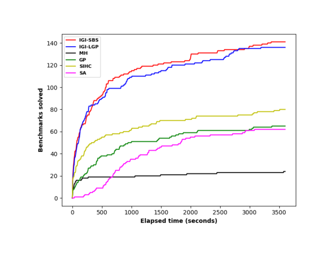
(a)

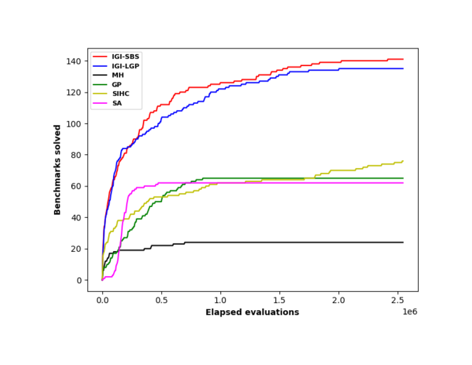
(b)

Figure 9: a) Number of benchmarks solved versus the computation time; (b) Number of benchmarks solved versus the number of evaluations in the list manipulation domain.

In Figure 9, we plot the number of benchmarks solved versus computation time (Figure 9LABEL:sub@fig-lisptime) and the number of evaluations (Figure 9LABEL:sub@fig-lispeval) for each algorithm. Compared to the baselines, the number of benchmarks solved by IGI-SBS or IGI-LGP increases more steadily with elapsed time/evaluations. For MH, almost all the solutions are found during the very early period of the search. Considering that MH searches for progressively larger programs, this implies that its search mechanism is inadequate for synthesizing larger programs. Note that SA gets stuck after a relatively small number of evaluations (i.e., about $5\times 10^{5}$), but these evaluations cost most of the budget time (i.e., about 3000 seconds). This implies that SA tends to examine larger programs whose execution times are longer.

Table 4: Results for 10 hard benchmarks (in the list manipulation domain) that are randomly chosen. The data indicates the number of successful runs out of 50. Best performance is shown in bold.

Benchmarks	IGI-SBS	IGI-LGP	MH	GP	SIHC	SA
L15	20	24	0	1	0	0
L53	20	14	0	0	0	0
L82	4	8	0	1	0	7
L129	37	36	0	1	0	0
L172	15	12	0	0	0	0
L179	29	35	0	12	0	10
L180	26	32	0	0	4	4
L183	30	39	4	13	1	0
L188	32	25	0	0	0	0
L197	32	28	0	0	0	0

Due to the stochastic nature of SPS techniques we measure the performance of each technique as the number of runs out of 50 that solve the benchmark, called success rate. Table 4 lists the success rates of each algorithm on 10 hard benchmarks. These benchmarks are randomly chosen out of the 200 benchmarks and can be solved by no more than three techniques, according to the results in Table 3. It can be seen from Table 4 that IGI-SBS and IGI-LGP perform similarly well and obtain the best success rates on some of the 10 benchmarks. IGI-SBS and IGI-LGP perform much better than all baselines except on L82 where SA is very competitive. On L53, L172, L188 and L197, IGI-SBS and IGI-LGP can achieve decent success rates, whereas all the baselines never succeed.

In summary, the IGI algorithms clearly outperform all the baselines in terms of scalability in the list manipulation domain with overall better solution quality. Moreover, they also have an overwhelming advantage in solving hard synthesis tasks.

IV.3 Results for String Transformation

Table 5 shows the main result in the string transformation domain. IGI-SBS and IGI-LGP solve the most number of benchmarks (i.e., 172 for both of them), followed by GP that solves 159. So IGI algorithms again outperform all the other algorithms in terms of scalability. Moreover, they are also superior to others in terms of synthesis time. In particular, IGI-SBS finds solutions in an average time of 73.39 seconds, whereas SIHC, the fastest baseline, consumes 128.16 seconds on average.

Table 5: Main result (in the string transformation domain) comparing the performance of all algorithms considered.

Statistics	IGI-SBS	IGI-LGP	MH	GP	SIHC	SA
Total solved	172	172	108	159	156	158
Fastest solved	63	50	2	5	51	3
Smallest solved	56	38	38	14	88	6
Average time	73.39	109.45	360.04	135.3	128.16	325.29
Median time	4.02	5.25	29.56	39.39	6.94	91.79
Average size	19.1	20.78	24.82	42.37	14.28	277.43
Median size	17.0	19.0	15.0	27.0	12.5	120.0

In terms of solution size, SA severely suffers from the code growth problem and average solution size reaches over 277, possibly due to the same reason as in Section IV.2. GP suffers from a similar problem with average and median sizes of 42.37 and 27. IGI-SBS and IGI-LGP find solutions that are of comparable size to those by MH and SIHC, but are better in scalability.

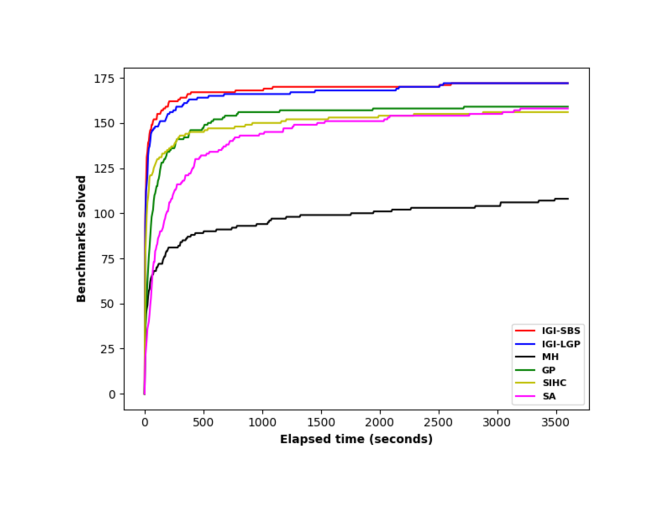
(a)

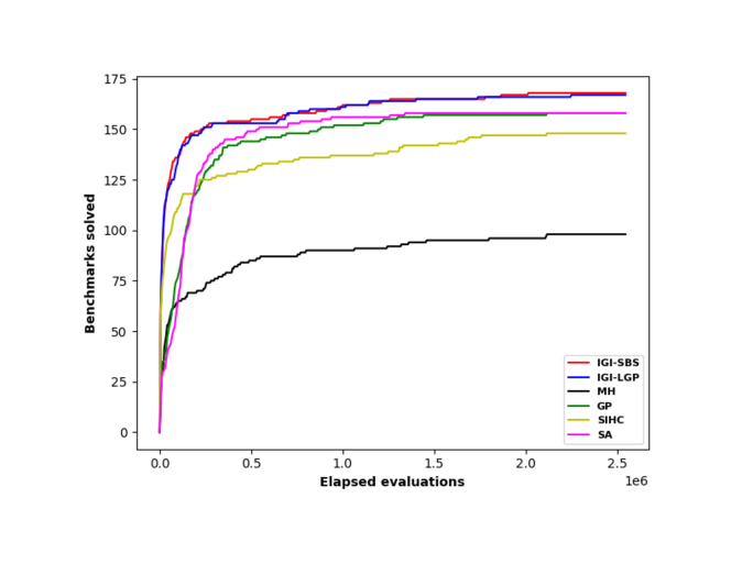
(b)

Figure 10: (a) Number of benchmarks solved versus the computation time; (b) Number of benchmarks solved versus the number of evaluations in the string transformation domain.

Figure 10 plots the number of benchmarks solved with the increasing of computational time (Figure 10LABEL:sub@fig-sliatime) and evaluations (Figure 10LABEL:sub@fig-sliaeval). Unlike in the list manipulation domain, the trajectories of IGI-SBS and IGI-LGP start steep and almost flatten very quickly, indicating that most of benchmarks in this domain do not pose great challenge to IGI.

Table 6: Results for 10 hard benchmarks (in the string transformation domain) that are randomly chosen, where $n$ shows the number of examples for each benchmark. The data indicates the number of successful runs out of 50. Best performance is shown in bold.

Benchmarks	$n$	IGI-SBS	IGI-LGP	MH	GP	SIHC	SA
31753108	3	50	50	0	28	1	22
44789427	4	50	50	0	35	12	42
exceljet2	3	50	50	0	39	9	18
enwfts	4	44	36	0	14	0	23
ewtbwsc	3	50	49	0	47	6	10
gmnffn	4	50	49	0	22	0	18
p10lr	400	46	42	9	26	18	34
stsasc	4	50	50	0	43	1	31
sncfc	3	46	45	0	48	10	41
univ_4	8	49	42	0	32	1	27

To further examine the performance of IGI, we select 10 hard benchmarks in the same way as we do in the list manipulation domain. Table 6 shows the success rates for each algorithm on these 10 benchmarks. From Table 6, IGI-SBS always succeeds in 6 benchmarks, while IGI-LGP always succeeds in 4. Both IGI-SBS and IGI-LGP achieve higher success rates than all the baselines on all the benchmarks except on sncfc where GP is slightly better. MH performs very poorly, which always fails in 9 out of 10 benchmarks. It seems that although SIHC is very competitive to GP and SA in terms of the number of benchmarks solved, it generally performs worse than GP and SA on hard benchmarks. The similar phenomenon can be observed in the list manipulation domain. This implies that it is more difficult for the simple search mechanism of SIHC to adapt to hard synthesis tasks that may have complex fitness landscapes.

In summary, IGI algorithms perform better than all the other algorithms in terms of scalability in the string transformation domain, without sacrificing the solution quality. In addition, they spend less average time to find solution programs, and also have much stronger ability to address hard synthesis tasks.

IV.4 On the Issue of Generalization

Although the issue of generalization is not the focus of this paper, it is interesting to see how well the solution programs found by IGI algorithms generalize to unseen input-output examples. We generated 100 additional input-output examples for each of the 200 benchmarks in the list manipulation domain using the corresponding oracle programs. Note that this cannot be done in the string transformation domain since oracle programs are unknown for those benchmarks.

Table 7: Percentage of solution programs that can generalize to 100 hold-out input-output examples.

Statistics	IGI-SBS	IGI-LGP	MH	GP	SIHC	SA
Total solved	141	136	24	65	80	62
Generalizable	133	122	23	57	68	51
Percentage (%)	94.33	89.71	95.83	87.69	85	82.26

Table 7 reports the percentage of solution programs that can generalize to 100 hold-out input-output examples for each considered algorithm. It can be seen that the IGI algorithms have better generalization ability than GP, SIHC and SA. This also implies that the better scalability of IGI is not due to overfitting on given input-output examples. MH achieves the highest generalization percentage, but from a small basis as it only solves 24 relatively easy tasks with overfitting less likely to occur. It is worth mentioning that in our experiments all algorithms considered stop searching once a solution is found. We can further alleviate overfitting by letting the algorithm return all solution programs found within the time budget and then choose the smallest one among them.

V Related Work

Program synthesis is an active research topic including a large and diverse body of work, such as enumerative program synthesis alur2017scaling ; lee2018accelerating ; huang2020reconciling ; lee2021combining , constraint-based program synthesis solar2008program ; srivastava2010program ; jha2010oracle and neural program synthesis devlin2017robustfill ; parisotto2017neuro ; hong2021latent ; chen2021evaluating . In what follows, we review some prior work on stochastic program synthesis that is most closely related to our proposed IGI.

Metropolis-Hastings algorithm. This line of research started from STOKE schkufza2013stochastic , which tackles superoptimization problems using a stochastic search strategy known as Metropolis-Hastings (MH). Due to the surprisingly good performance of STOKE on superoptimization, it had stirred great interest with its publication and was regarded as a timely and significant contribution gulwani2016technical to program synthesis at that time. Alur et al. alur2013syntax adapted STOKE and introduced a MH approach over programs represented by trees. This MH approach participated in SyGuS competitions 2014–2016 sygus2014 , but it did not achieve very competitive performance compared to other categories of techniques. Since then, the enthusiasm of researchers for stochastic synthesis seemed to drop and there was no stochastic solver participating in SyGuS competitions in the following years. Recently, several studies have been conducted to enhance the performance of STOKE. For example, Bunel et al. bunel2017learning proposed to learn the proposal distribution in STOKE parameterized by a neural network, which is expected to better exploit the power of MH; Koenig et al. koenig2021adaptive proposed an effective adaptive restart algorithm for addressing a limitation in STOKE where the search often progresses via a series of plateaus. However, these enhancements have mostly targeted superoptimization, and it is still unclear how to make them amenable to stochastic search over trees.

Genetic programming. Genetic programming (GP) koza1992genetic ; banzhaf1998genetic ; poli2008field has a much longer history than Metropolis-Hastings algorithm for the purpose of program synthesis. Indeed, achieving automatic programming is arguably the most aspirational goal in the field of GP o2019automatic . In canonical GP, the variation operations are implemented via crossover and mutation. Borrowing ideas from estimation of distribution algorithms (EDAs) larranaga2001estimation , an interesting alternative is to replace such variation operations with the process of sampling from a probability distribution salustowicz1997probabilistic ; sastry2003probabilistic ; yanai2003estimation . One typical example in this family of GP is probabilistic incremental program evolution (PIPE) salustowicz1997probabilistic , where the population is replaced by a hierarchy of probability tables with the tree structure. Although EDA-based GP approaches are appealing, they usually fail to offer significant performance gains over standard tree-based GP poli2008field , which remains to be investigated. It is known that the most widespread type of GP expresses programs as syntax trees, but there are other GP based program synthesizers which use different program representations. PushGP spector2002genetic and grammar-guided GP (GGGP) mckay2010grammar are among the most representative ones. PushGP evolves programs expressed in the Push programming language, which supports different data types by providing a stack for each data type as well as for the code that is executed. Recent studies around PushGP focus on designing new mutation operators helmuth2018program and parent selection methods helmuth2016lexicase ; helmuth2020benchmarking in order to further improve its performance. GGGP can either use the derivation tree whigham1995grammatically or a linear genome o2001grammatical as its program representation, which can be mapped to a resulting program via the context-free grammar. Recently, some work on GGGP has paid attention to grammar design forstenlechner2017grammar , generalizability sobania2021generalizability and the quality of generated code sobania2019teaching ; hemberg2019domain .

Stochastic local search. Although stochastic local search (SLS) hoos2004stochastic has been used extensively for combinatorial problems, there is surprisingly few research on SLS for program synthesis. The most notable work in this direction is O’Reilly’s PhD thesis o1995analysis , where stochastic iterated hill climbing (SIHC) and simulated annealing (SA) were investigated for solving program discovery problems. Her results indicate that SIHC and SA are generally comparable to GP and even sometimes outperform GP. In addition to this work, there are some other research efforts on SLS that target a specific synthesis problem. For example, Nguyen et al. nguyen2014automatic proposed to evolve dispatching rules in job-sop scheduling via iterated local search; Kantor et al. kantor2021simulated presented simulated annealing using the interaction-transformation representation for symbolic regression.

But all these methods have not (yet) succeeded in bringing into being a comprehensive methodology for program synthesis. So it remains to be seen which technique has the most power and will be adopted by the wider community.

VI Conclusion

In this paper, we have proposed IGI, a new framework for stochastic program synthesis. Inspired by the process of human programming, IGI considers a sequence of program improvements by iteratively searching for modifications to the current reference program. In terms of solution representation, IGI uses a differential code representation that will undergo epochs of evolution under the control of input-output examples. IGI can therefore also be seen as a kind of generative or developmental genetic programming koza2010human ; eiben2015evolutionary , which allows the reuse of code and helps to scale up the complexity of evolved programs. Experimental results on two different application domains have demonstrated the clear advantage of IGI over several representative SPS techniques in terms of scalability and solution quality.

In the future, we will investigate how to extend IGI to popular general-purpose programming languages chen2021evaluating . It would also be interesting to use IGI as the symbolic search engine in neurosymbolic programming chaudhuri2021neurosymbolic .

Appendix A DSL for List Manipulation (DSL-LM)

This DSL is introduced in the DeepCoder paper balog2017deepcoder , which is inspired by query languages such as SQL. It contains a number of high-level functions that can be used to manipulate integer arrays or integers. In Tables 8 and 9 we list all of the functions of DSL-LM and give their symbols, argument types, return types and detailed descriptions. For each benchmark task in this domain, all these functions are available. Note that there are no constants in DSL-LM, and terminals are all from the program’s external inputs.

Table 8: Description of functions in the DSL-LM.

Symbol	Arguments	Return Type	Description
HEAD	$x$: Integer array	Integer	Return the first element of a given array $x$ (or
			NULL if $x$ is empty).
LAST	$x$: Integer array	Integer	Return the last element of a given array $x$ (or
			NULL if $x$ is empty).
TAKE	$n$: Integer;	Integer array	Given an integer $n$ and an array $x$, return the
	$x$: Integer array		array truncated after the $n$-th element. (If the
			length of $x$ is not larger than $n$, return $x$ without
			modification.)
DROP	$n$: Integer;	Integer array	Given an integer $n$ and an array $x$, return the
	$x$: Integer array		array with the first $n$ elements dropped. (If the
			length of x is not larger than $n$, return an empty
			array.)
ACCESS	$n$: Integer;	Integer	Given an integer $n$ and an array $x$, return the
	$x$: Integer array		($n+1$)-th element of $x$. (If the length of $x$ is not
			larger than $n$, return NULL.)
MINIMUM	$x$: Integer array	Integer	Return the minimum of a given array (or NULL
			if $x$ is empty).
MAXIMUM	$x$: Integer array	Integer	Return the maximum of a given array (or NULL
			if $x$ is empty).
REVERSE	$x$: Integer array	Integer array	Return the elements of a given array $x$ in reversed
			order.
SORT	$x$: Integer array	Integer array	Return the elements of a given array $x$ in
			non-decreasing order.
SUM	$x$: Integer array	Integer	Return the sum of the elements in a given array $x$.
MAPA1	$x$: Integer array	Integer array	Each element in a given array $x$ plus 1, and the
			modified array is returned.
MAPM1	$x$: Integer array	Integer array	Each element in a given array $x$ minus 1, and the
			modified array is returned.
MAPT2	$x$: Integer array	Integer array	Each element in a given array $x$ is multiplied by 2,
			and the modified array is returned.
MAPT3	$x$: Integer array	Integer array	Each element in a given array $x$ is multiplied by 3,
			and the modified array is returned.
MAPT4	$x$: Integer array	Integer array	Each element in a given array $x$ is multiplied by 4,
			and the modified array is returned.
MAPD2	$x$: Integer array	Integer array	Each element in a given array $x$ divided by 2 (fractions
			are rounded down), and the modified array is returned.
MAPD3	$x$: Integer array	Integer array	Each element in a given array $x$ divided by 3 (fractions
			are rounded down), and the modified array is returned.
MAPD4	$x$: Integer array	Integer array	Each element in a given array $x$ divided by 4 (fractions
			are rounded down), and the modified array is returned.
MAPV1	$x$: Integer array	Integer array	Each element in a given array $x$ is multiplied by -1,
			and the modified array is returned.
MAPP2	$x$: Integer array	Integer array	Each element in a given array $x$ is multiplied by
			itself, and the modified array is returned.
FILG0	$x$: Integer array	Integer array	Return the elements of a given array $x$ that are larger
			than 0 in their original order.
FILL0	$x$: Integer array	Integer array	Return the elements of a given array $x$ that are less
			than 0 in their original order.
FILEV	$x$: Integer array	Integer array	Return the elements of a given array $x$ that are even
			in their original order.
FILOD	$x$: Integer array	Integer array	Return the elements of a given array $x$ that are odd
			in their original order.
COUG0	$x$: Integer array	Integer	Return the number of elements in a given array $x$
			that is larger than 0.
COUL0	$x$: Integer array	Integer	Return the number of elements in a given array $x$
			that is less than 0.
COUEV	$x$: Integer array	Integer	Return the number of elements in a given array $x$
			that is even.
COUOD	$x$: Integer array	Integer	Return the number of elements in a given array $x$
			that is odd.

Table 9: Description of functions in the DSL-LM (continued).

Symbol	Arguments	Return Type	Description
ZIPSUM	$x$: Integer array	Integer array	Return an array $z$ with length $n$ where
	$y$: Integer array		$z[i]=x[i]+y[i]$, $i=0,1,\ldots n-1$ and $n$ is
			the minimum of the lengths of $x$ and $y$.
ZIPDIF	$x$: Integer array	Integer array	Return an array $z$ with length $n$ where
	$y$: Integer array		$z[i]=x[i]-y[i]$, $i=0,1,\ldots n-1$ and $n$ is
			the minimum of the lengths of $x$ and $y$.
ZIPMUL	$x$: Integer array	Integer array	Return an array $z$ with length $n$ where
	$y$: Integer array		$z[i]=x[i]*y[i]$, $i=0,1,\ldots n-1$ and $n$ is
			the minimum of the lengths of $x$ and $y$.
ZIPMAX	$x$: Integer array	Integer array	Return an array $z$ with length $n$ where
	$y$: Integer array		$z[i]=\max\{x[i],y[i]\}$, $i=0,1,\ldots n-1$
			and $n$ is the minimum of the lengths of $x$ and $y$.
ZIPMIN	$x$: Integer array	Integer array	Return an array $z$ with length $n$ where
	$y$: Integer array		$z[i]=\min\{x[i],y[i]\}$, $i=0,1,\ldots n-1$
			and $n$ is the minimum of the lengths of $x$ and $y$.
SCANSUM	$x$: Integer array	Integer array	Returns an array $y$ of the same length as $x$ and
			with its content defined by the recurrence:
			$y[0]=x[0]$, $y[i]=y[i-1]+x[i]$, for $i\geq 1$.
SCANDIF	$x$: Integer array	Integer array	Returns an array $y$ of the same length as $x$ and
			with its content defined by the recurrence:
			$y[0]=x[0]$, $y[i]=y[i-1]-x[i]$, for $i\geq 1$.
SCANMUL	$x$: Integer array	Integer array	Returns an array $y$ of the same length as $x$ and
			with its content defined by the recurrence:
			$y[0]=x[0]$, $y[i]=y[i-1]*x[i]$, for $i\geq 1$.
SCANMAX	$x$: Integer array	Integer array	Returns an array $y$ of the same length as $x$ and
			with its content defined by the recurrence:
			$y[0]=x[0]$, $y[i]=\max\{y[i-1],x[i]\}$, for $i\geq 1$.
SCANMIN	$x$: Integer array	Integer array	Returns an array $y$ of the same length as $x$ and
			with its content defined by the recurrence:
			$y[0]=x[0]$, $y[i]=\min\{y[i-1],x[i]\}$, for $i\geq 1$.

Appendix B DSL for String Transformation (DSL-ST)

This DSL is designed for the PBE-Strings track in the SyGuS competition sygus2014 . Table 10 describes all of the functions of DSL-ST in detail. Terminals include constants and the program’s external inputs. For each task of the SyGuS benchmarks the definition file specifies – besides the input-output examples – what functions in Table 10 are used and provides some string, integer and Boolean constants.

Table 10: Description of functions in the DSL-ST.

Symbol	Arguments	Return Type	Description
CAT	$s$: String	String	Concatenate the strings $s$ and $t$, and return
	$t$: String		the combined string.
REP	$s$: String	String	Return a copy of the string $s$ where the first
	$t$: String		occurrence of a substring $t$ is replaced with
	$r$: String		another substring $r$.
AT	$s$: String	String	Return the string containing a single character
	$i$: Integer		at index $i$ in $s$, i.e., $s[i]$. (If $i<0$ or $i$ is no smaller
			than the length of $s$, return an empty string.)
ITS	$x$: Integer	String	If integer $x$ is not smaller than 0, convert $x$ into
			the string and return the string. Otherwise,
			return an empty string.
SITE	$b$: Boolean	String	If $b$ is true, return $s$, otherwise return $t$.
	$s$: String
	$t$: String
SUBSTR	$s$: String	String	Return the substring of a given string $s$ with the
	$i$: Integer		start index $i$ and the end index $\min\{n,i+j\}-1$,
	$j$: Integer		where $n$ is the length of $s$. (If $i<0$ or $j<0$ or
			$i\geq n$, return an empty string.)
ADD	$x$: Integer	Integer	Return the sum of integers $x$ and $y$.
	$y$: Integer
SUB	$x$: Integer	Integer	Return the difference between integers $x$ and $y$.
	$y$: Integer
LEN	$s$: String	Integer	Return the length of a given string $s$.
STI	$s$: String	Integer	If all characters in the string $s$ are digits, convert
			$s$ into the integer and return the integer.
			Otherwise return $-1$.
IITE	$b$: Boolean	Integer	If $b$ is true, return $x$, otherwise return $y$.
	$x$: Integer
	$y$: Integer
IND	$s$: String	Integer	Search the string $t$ in the substring of $s$ that starts at
	$t$: String		index $i$ and ends at index $n-1$, where $n$ is the length
	$i$: Integer		of $s$, and return the lowest index in $s$ where $t$ is found.
			(If $i<0$ or $i\geq n$ or $t$ is not found in $s$, return $-1$.)
EQ	$x$: Integer	Boolean	If $x$ equals to $y$, return true, otherwise return
	$y$: Integer		false.
PRF	$s$: String	Boolean	If $s$ is the prefix of $t$, return true, otherwise return
	$t$: String		false.
SUF	$s$: String	Boolean	If $s$ is the suffix of $t$, return true, otherwise return
	$t$: String		false.
CONT	$s$: String	Boolean	If $t$ is found in $s$, return true, otherwise return
	$t$: String		false.

Appendix C Parameter Selection

Key parameters of each algorithm were tuned by performing grid search on two hard synthesis tasks from the list and string transformation domains. For each parameter combination of an algorithm, we performed 10 independent runs using a timeout criterion of 20 minutes on the two tasks. We ranked all parameter combinations of an algorithm according to the average maximum fitness achieved over 10 runs and selected the parameter combination with the lowest average rank over the two tasks. For IGI-SBS, the space of parameters considered is beam width $\in\{25,50,100\}$, number of successors for each patch is $\in\{5,10,20\}$, the maximum length of patches considered is $\in\{2,3,4\}$, and tournament size is $\in\{2,5,8\}$, for a total of 81 combinations. For IGI-LGP, the space of parameters considered is population size $\in\{50*i|i=1,\ldots,8\}$, maximum number of generations in each epoch is $\in\{5,10,20\}$ and tournament size is $\in\{2,5,8\}$ for a total of 72 combinations. For MH, the space of parameters considered is switch probability $\in\{0.002*i|i=1,2,\ldots,10\}$ and smoothing constant $\in\{0.1,0.3,0.5,0.7,0.9\}$ for a total of 50 combinations. For GP, the space of parameters considered is population size $\in\{5000,10000,20000\}$, crossover probability $\in\{0.8,0.9,1.0\}$, mutation probability (per node) $\in\{0.05,0.08,0.1\}$ and tournament size $\in\{2,5,8\}$ for a total of 81 combinations. For SIHC, the space of parameters considered is the maximum number of mutations $\in\{500*i|i=1,2,\ldots,40\}$ for a total of 40 combinations. For SA, the space of parameters considered is final temperature $\in\{0.0001,0.0005,0.001,0.005,0.01\}$ and stepsize $\in\{500*i|i=1,2,\ldots 10\}$ for a total of 50 combinations.

The final tuned parameters for all algorithms considered are shown in Tables 11 to 16. These parameters are used throughout our experiments.

Table 11: Parameter setting of IGI-SBS.

Parameter	Value
Beam width ($B$)	50
Number of successors of each patch ($C$)	5
Maximum length of patches considered ($L_{\max}$)	3
Tournament size	2
Number of initial programs ($K$)	$B\times C\times L_{\max}$
Number of perturbations ($M$)	200
Minimum perturbation strength ($S_{\min}$)	4
Minimum depth of initial programs ($d_{\min}$)	2
Maximum depth of initial programs ($d_{\max}$)	4

Table 12: Parameter setting of IGI-LGP.

Parameter	Value
Population size ($N$)	100
Maximum generations ($G$)	5
Tournament size	2
Crossover probability	1.0
Mutation probability	1.0
Number of initial programs ($K$)	$N\times G$
Number of perturbations ($M$)	200
Minimum perturbation strength ($S_{\min}$)	4
Minimum depth of initial programs ($d_{\min}$)	2
Maximum depth of initial programs ($d_{\max}$)	4

Table 13: Parameter setting of MH.

Parameter	Value
Switch probability ($p_{m}$)	0.006
Smoothing constant ($\beta$)	0.7
Maximum allowed depth of programs	30

Table 14: Parameter setting of GP.

Parameter	Value
Population size	20000
Crossover probability	0.9
Mutation probability (per node)	0.1
Tournament size	2
Minimum depth of initial programs ($d_{\min}$)	2
Maximum depth of initial programs ($d_{\max}$)	4
Maximum allowed depth of programs	30

Table 15: Parameter setting of SIHC.

Parameter	Value
Maximum number of mutations ($T_{\max}$)	500
Minimum depth of initial programs ($d_{\min}$)	2
Maximum depth of initial programs ($d_{\max}$)	4
Maximum allowed depth of programs	30

Table 16: Parameter setting of SA.

Parameter	Value
Starting temperature	1.5
Final temperature	0.001
Stepsize	500
Minimum depth of initial programs ($d_{\min}$)	2
Maximum depth of initial programs ($d_{\max}$)	4
Maximum allowed depth of programs	30