Low SNR Multiframe Registration for Cubesats
Abstract
We present a registration algorithm which jointly estimates motion and the ground truth image from a set of noisy frames under rigid, constant translation. The algorithm is non-iterative and needs no hyperparameter tuning. It requires a fixed number of FFT, multiplication, and downsampling operations for a given input size, enabling fast implementation on embedded platforms like cubesats where on-board image fusion can greatly save on limited downlink bandwidth. The algorithm is optimal in the maximum likelihood sense for additive white Gaussian noise and non-stationary Gaussian approximations of Poisson noise. Accurate registration is achieved for very low SNR, even when visible features are below the noise floor.
Index Terms— astronomy, image registration, maximum likelihood, low SNR, motion estimation, embedded signal processing
1 Introduction
Image alignment, or image registration is a classic problem in the field of image processing involving the alignment of an image set or image sequence that has been acquired at different times, sensors, or viewpoints. Registration is an important preprocessing step in image processing pipelines involving change detection, image mosaicing, denoising, and super-resolution with applications in medical imaging [1], computer vision tasks [2] like segmentation or classification, military surveillance [3], and remote-sensing.
Registration techniques have been broadly classified into area-based and feature-based categories [4] [5]. Feature-based approaches rely on detection of keypoints (points, edges, regions, corners, local gradients, etc.) which are then corresponded to estimate motion transformation parameters. In astronomy, these methods tend to be focused on matching starfields [6] [7] or geophysical imagery [8] and the keypoint detection algorithms generally perform poorly for astronomical imagery which is smoothly varying or very low SNR. In these situations, area-based methods which take a statistical approach are more appropriate.
There have been several publications which propose a maximum likelihood (ML) approach to registration, starting with Bradley [9], who showed an equivalence between ML and least squares estimates along with Kumar [10] specifically for registration under additive white Gaussian noise (AWGN). Later, Mort & Srinath [11] developed an ML subpixel registration algorithm for pairs of Nyquist-sampled images. Guillaume, et al. [12] and Gratadour et al. [13] developed a method for a sequence of low SNR astronomical image frames under Poisson and Gaussian noise.
Our algorithm 111https://github.com/evidlo/multiml is most closely related to to the method devised by Gratadour et al. [13], who applied their algorithm to images from an infrared galactic source taken from a ground based telescope. They derive a cost function for an image sequence with unconstrained motion, then used an iterative conjugate gradient minimization requiring evaluation of the cost gradient along with hyperparameter tuning.
We have discovered that when this cost function is constrained to constant interframe motion, the global optimum can be found without the use of an iterative minimizer, requiring only image addition, multiplication, downscaling, and FFT operations which are easily implementable on embedded platforms like FPGAs or are already available as off-the-shelf IP cores [14], making on-board registration and fusion much simpler.
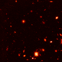
Noiseless frame
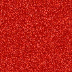
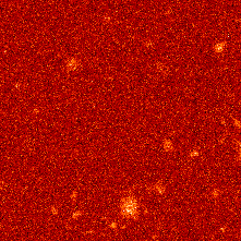
Noisy frame. -25dB SNR
Our algorithm was conceived for the upcoming VISORS mission, a technology demonstration of a diffractive optical element known as a photon sieve designed to study the solar corona at high resolution [15] [16]. VISORS features two freely-flying cubesats where the apparent motion of the scene is approximately constant translation during the 10 second science capture window. This stronger assumption about the motion allows us to register image frames at lower SNRs than more general methods, even when visible features are significantly below the noise floor, as in Fig. 1. Additionally, registering and fusing images sequences on-board rather than on the ground can significantly increase the science return with the limited data downlink budget available on VISORS.
In the next few sections, we provide an observation model describing motion of the frames and noise, a description of the algorithm and implementation for fast computation, a proof of optimality under the described motion and noise model, and experimental results comparing registration error of the algorithm with other area-based astronomical registration methods.
2 Observation Model and Algorithm
Let be an ordered sequence of noisy observed frames captured at a constant frame rate with constant drift between frames of pixels. Each frame has an offset of relative to some unknown ground truth.
For each , we have
| (1) |
where is a translation operator by vector pixels, is a Nyquist sampled version of the ground truth scene (also known as the reference image), and is measurement noise. We have assumed to be a circular translation for ease of derivation, which holds approximately true for small motion vector relative to the size of a frame and has been addressed in other literature for larger values of by windowing the images in a preprocessing step [17].
Note that if blurring induced by motion and the imaging system is spatially and temporally invariant, this constant PSF may be incorporated into and accounted for after registration.
The maximum likelihood solution is given by
| (2) |
which consists of a series of correlations denoted by , two summations, and a downsampling by . Taking over the resultant surface yields the maximum likelihood estimate of the motion, . The number of multiplications required is on the order of
The algorithm can be accelerated by performing correlations in the frequency domain and precomputing the Fourier transforms of the images with FFTs:
| (3) |
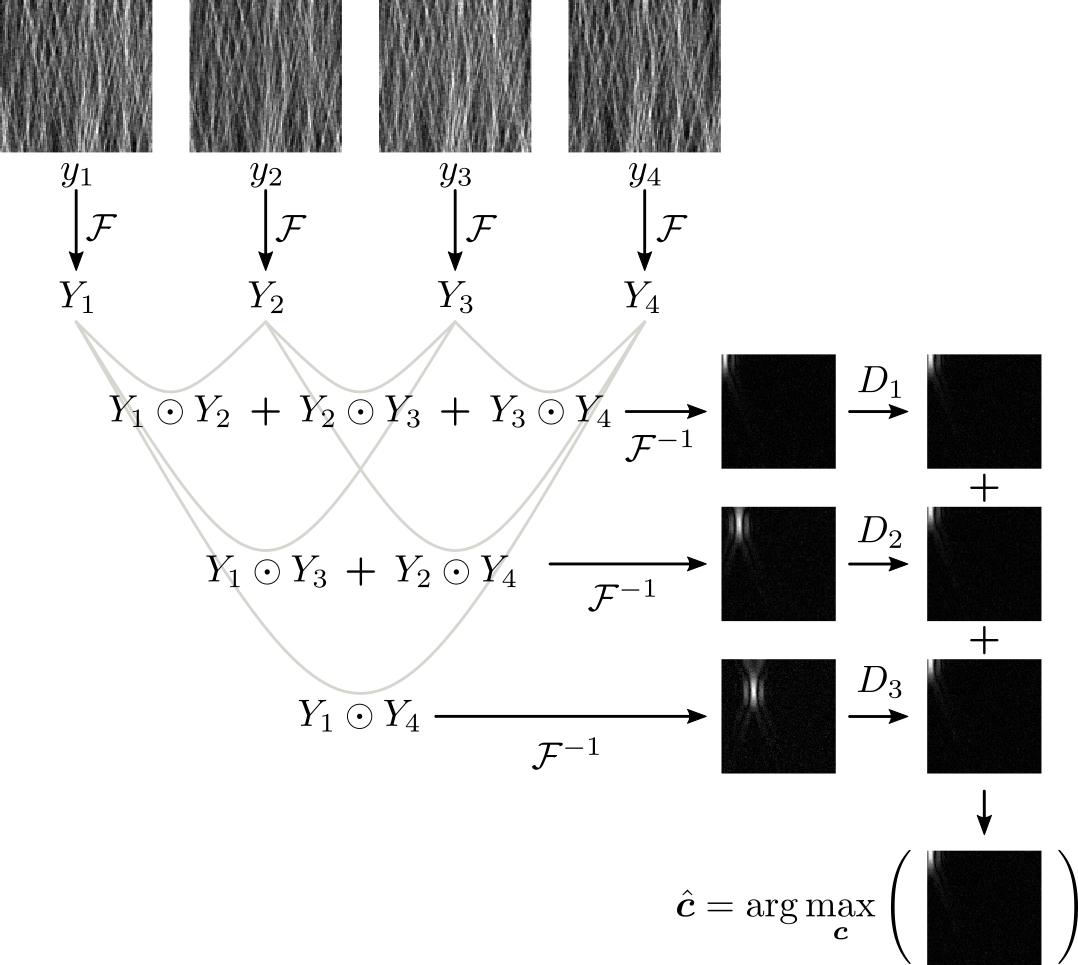
where is a downsample operator by pixels (with zero padding to maintain shape), is the inverse FFT, is the Fourier transform of , and is the elementwise product operator. The new complexity is . The algorithm can be broken into four steps, shown below and illustrated graphically in Fig. 2.
-
1.
Precompute image Fourier transforms:
-
2.
Compute image correlations and sum into groups by degree of separation :
-
3.
Downsample correlation groups by degree of separation and sum:
-
4.
Take the argmax of the resultant surface to find the estimate
3 Proof of ML Optimality
The proof of optimality is presented in 3 parts:
-
1.
Derive the expression for likelihood maximization over and
-
2.
Derive the most likely value for as a function of
-
3.
Show that the log-likelihood solution consists of a sum of downsampled cross correlations
Without loss of generality, we assume the observed frames to be one dimensional vectors of length and that drift is a scalar.
Given the observation model
assume is additive white Gaussian noise with variance . We note that the proof may be extended to non-stationary noise, similar to [13], but omit it here for brevity.
The log-likelihood of having a particular and given observation sequence is
| (4) |
We will take the derivative of the expression denoted cost(, ) in Equation 4 with respect to the th element of to eliminate minimization over .
| (5) |
This is simply the sum of the motion-corrected noisy frames. Plugging this into the cost function, we obtain an expression that depends only on . Expanding and eliminating constant terms, we get
Examining the first term in the cost function, we see it is simply a downsampled correlation between and .
Similarly, the second term can be manipulated into a cross correlation.
Combining the two terms, we arrive at
which is identical to Equation 2 given in the previous section.
4 Experimental Results
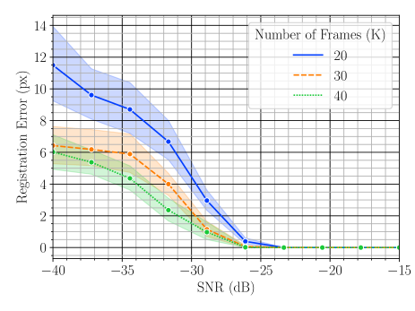
To evaluate performance of the algorithm, we generated a series of simulated pixel noisy frames from Hubble deep field images (shown in Fig. 3a) according to the motion and noise model given in Equation 1. We estimated interframe motion using our algorithm in Equation 3 and then coadded the corrected frames as in Equation 5 to obtain the reconstruction in Fig. 3b.
We repeated this experiment with various noise levels and number of frames for 50 trials each with a random motion vector and noise. As shown in Fig. 4 and corroborated in [13], the registration error decreases with increasing number of frames and is able to obtain less than 1 pixel of mean absolute registration error at -25dB measurement noise for frames, and the same at -30dB for .
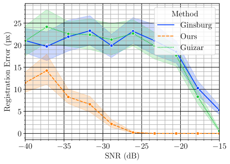
Next, we compared registration performance on astronomical data against another area-based registration method provided by Ginsburg et al. [18], originally used for registering images of cosmic dust in infrared and also against a pairwise version of the algorithm given in [guizar2008efficient]. Since these algorithms have a non-constant motion model, we project their motion estimates to the nearest constant, rigid motion estimate for a fairer comparison. Again, the experiment was repeated for 50 trials with a randomized motion vector and noise realization.
Fig. 5 shows that our algorithm is able to successfully register images at over 10dB lower SNR.
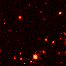
(a) Ground truth
(b) Reconstruction
5 Summary and Conclusion
In this manuscript, we presented a multiframe registration algorithm for constant rigid motion. We showed that the algorithm can be realized without iterative methods or parameter tuning, and that the algorithm is optimal in the maximum likelihood sense. We characterized the algorithm for various noise levels and image sequence lengths.
The algorithm may be directly extended to the subpixel domain by applying the techniques described in [guizar2008efficient]. It is also possible to handle constant scaling and rotation using the Log-Polar transform as described in [19], but this requires interpolation that may be expensive on embedded platforms.
The algorithm is useful in settings where motion is constant and rigid, images are low SNR, or a straightforward implementation on an embedded system is needed.
References
- [1] William M Wells III, Paul Viola, Hideki Atsumi, Shin Nakajima, and Ron Kikinis, “Multi-modal volume registration by maximization of mutual information,” Medical image analysis, vol. 1, no. 1, pp. 35–51, 1996.
- [2] Jiri Matas, Ondrej Chum, Martin Urban, and Tomás Pajdla, “Robust wide-baseline stereo from maximally stable extremal regions,” Image and Vision Computing, vol. 22, no. 10, pp. 761–767, 2004.
- [3] Alan C Bovik, Handbook of Image and Video Processing, Academic Press, 2010.
- [4] Barbara Zitova and Jan Flusser, “Image registration methods: a survey,” Image and vision computing, vol. 21, no. 11, pp. 977–1000, 2003.
- [5] Lisa Gottesfeld Brown, “A survey of image registration techniques,” ACM computing surveys (CSUR), vol. 24, no. 4, pp. 325–376, 1992.
- [6] Martin Beroiz, Juan B Cabral, and Bruno Sanchez, “Astroalign: A python module for astronomical image registration,” Astronomy and Computing, vol. 32, pp. 100384, 2020.
- [7] Dustin Lang, David W Hogg, Keir Mierle, Michael Blanton, and Sam Roweis, “Astrometry. net: Blind astrometric calibration of arbitrary astronomical images,” The astronomical journal, vol. 139, no. 5, pp. 1782, 2010.
- [8] Jianglin Ma, Jonathan Cheung-Wai Chan, and Frank Canters, “Fully automatic subpixel image registration of multiangle chris/proba data,” IEEE transactions on geoscience and remote sensing, vol. 48, no. 7, pp. 2829–2839, 2010.
- [9] Edwin L Bradley, “The equivalence of maximum likelihood and weighted least squares estimates in the exponential family,” Journal of the American Statistical Association, vol. 68, no. 341, pp. 199–200, 1973.
- [10] BVK Vijaya Kumar, Fred M Dickey, and John M DeLaurentis, “Correlation filters minimizing peak location errors,” JOSA A, vol. 9, no. 5, pp. 678–682, 1992.
- [11] Michael S Mort and MD Srinath, “Maximum likelihood image registration with subpixel accuracy,” in Applications of digital Image Processing XI. SPIE, 1988, vol. 974, pp. 38–45.
- [12] Mireille Guillaume, Pierre Melon, Philippe Réfrégier, and Antoine Llebaria, “Maximum-likelihood estimation of an astronomical image from a sequence at low photon levels,” JOSA A, vol. 15, no. 11, pp. 2841–2848, 1998.
- [13] D Gratadour, LM Mugnier, and D Rouan, “Sub-pixel image registration with a maximum likelihood estimator-application to the first adaptive optics observations of arp 220 in the l band,” Astronomy & Astrophysics, vol. 443, no. 1, pp. 357–365, 2005.
- [14] Xilinx, “Fast fourier transform (fft),” https://www.xilinx.com/products/intellectual-property/fft.html#overview.
- [15] Athreya Gundamraj, Rohan Thatavarthi, Christopher Carter, E Glenn Lightsey, Adam Koenig, and Simone D’Amico, “Preliminary design of a distributed telescope cubesat formation for coronal observations,” in AIAA Scitech 2021 Forum, 2021, p. 0422.
- [16] Adam Koenig, Simone D’Amico, and E Glenn Lightsey, “Formation flying orbit and control concept for the visors mission,” in AIAA Scitech 2021 Forum, 2021, p. 0423.
- [17] Stephen C Cain, Majeed M Hayat, and Ernest E Armstrong, “Projection-based image registration in the presence of fixed-pattern noise,” IEEE transactions on image processing, vol. 10, no. 12, pp. 1860–1872, 2001.
- [18] Adam Ginsburg, Jason Glenn, Erik Rosolowsky, Timothy P Ellsworth-Bowers, Cara Battersby, Miranda Dunham, Manuel Merello, Yancy Shirley, John Bally, Neal J Evans II, et al., “The bolocam galactic plane survey. ix. data release 2 and outer galaxy extension,” The Astrophysical Journal Supplement Series, vol. 208, no. 2, pp. 14, 2013.
- [19] B Srinivasa Reddy and Biswanath N Chatterji, “An fft-based technique for translation, rotation, and scale-invariant image registration,” IEEE transactions on image processing, vol. 5, no. 8, pp. 1266–1271, 1996.