Homeostatic and adaptive energetics:
Nonequilibrium fluctuations beyond detailed balance in voltage-gated ion channels

Homeostatic and adaptive energetics:
Nonequilibrium fluctuations beyond detailed balance in voltage-gated ion channels

Abstract

Stochastic thermodynamics has largely succeeded in characterizing both equilibrium and far-from-equilibrium phenomena. Yet many opportunities remain for application to mesoscopic complex systems—especially biological ones—whose effective dynamics often violate detailed balance and whose microscopic degrees of freedom are often unknown or intractable. After reviewing excess and housekeeping energetics—the adaptive and homeostatic components of a system’s dissipation—we extend stochastic thermodynamics with a trajectory class fluctuation theorem for nonequilibrium steady-state, nondetailed-balanced complex systems. We then take up the neurobiological examples of voltage-gated sodium and potassium ion channels to apply and illustrate the theory, elucidating their nonequilibrium behavior under a biophysically plausible action potential drive. These results uncover challenges for future experiments and highlight the progress possible understanding the thermodynamics of complex systems—without exhaustive knowledge of every underlying degree of freedom.

I Introduction

Nonequilbrium phenomena pervade nature: In their many forms, energy gradients send hurricanes and wildfires to ravage, volcanoes to form and erupt, life to emerge. Mesoscopic complex systems—a planetary climate, forest ecosystems, the human body—consist of microscopic degrees of freedom that are inaccessible, intractable, or simply unknown. In point of fact, the human body’s biochemistry relies essentially on out-of-equilibrium dynamics to function, adapt, and maintain homeostasis; its myriad degrees of freedom are only ever partially accessible. Similarly, mesoscopic and complex systems provide fertile grounds for honing and applying tools to analyze real-world nonequilibrium processes.

Describing energetic fluxes in complex systems—developing a suitable mesoscopic nonequilibrium thermodynamics—remains an ongoing challenge: mathematics and physics difficulties continue to hinder deeper understanding of how these systems operate and function. The following leverages and extends tools from stochastic thermodynamics and information theory to address these challenges. To demonstrate the techniques, it takes up two suitably complex, mesoscopic neurobiological systems: voltage-gated ion channels.

I.1 Nonequilibrium steady states

A system is typically called nonequilibrium in two distinct senses. The first, and most common, refers to nonequilibrium processes—say, induced by rapid environmental driving—wherein a system evolves through a series of transient configurations. When the environmental drive remains fixed, such a system remains out of equilibrium as it relaxes to some stationary distribution over its states, determined by the environmental parameters. If that stationary distribution corresponds to a thermodynamic equilibrium, we say the system possesses an equilibrium steady state (ESS), irrespective of its (perhaps highly nonequilibrium) driven, transient dynamics.

The second sense refers not to the transient behavior but to the nature of the stationary distributions: a nonequilbrium steady-state (NESS) system is one whose steady states are themselves out of thermodynamic equilibrium. This is simply achieved by contact with two heat baths at different temperatures. Rayleigh-Bénard convection Cros93a exemplifies this phenomenon: the temperature gradient between the top and bottom boundaries ensures a constant flux of energy through the fluid, from the hotter to the cooler, even when the gradient remains fixed indefinitely. In this case it is not enough to identify the energetic fluxes due to the system’s transient dynamics; we must also identify the energy required to maintain steady-state conditions in the first place.

NESSs appear even without multiple heat baths. For example, by optically dragging a bead through viscous fluid trepagnierExperimentalTestHatano2004 —an experimental realization of nonconservative force-driven Langevin dynamics—by coarse-graining microstates espositoStochasticThermodynamicsCoarse2012 ; or by contact with reservoirs of distinct electrochemical potentials—the case in virtually all common electrical circuits via Joule heating Gao21a . They emerge as well in the voltage-gated ion channels we consider.

A first attempt to give NESS systems a full thermodynamic framing defined the housekeeping heat $Q_{\textnormal{hk}}$ as the portion of the total heat $Q$ that maintains NESS conditions oonoSteadyStateThermodynamics1998 . (In this, the total heat is that energy exchanged between a system and its thermal environment, often idealized as a fixed-temperature bath.) What remains is the energy exchanged owing to the system’s relaxation to steady state, termed the excess heat $Q_{\textnormal{ex}}$:

$$Q=Q_{\textnormal{ex}}+Q_{\textnormal{hk}}\textnormal{.}$$ (1)

Contrast this with an equilibrium system’s steady states, which by definition exchange no net energy with the thermal environment. In this setting, $Q_{\textnormal{hk}}=0$ and so all dissipated heat is excess: $Q_{\textnormal{ex}}\to Q$. In other words, $Q_{\textnormal{ex}}$ in the NESS setting carries the same meaning as total heat $Q$ in the ESS setting, and vice versa.

I.2 Approach

Equilibrium thermodynamics and equilibrium statistical mechanics prove insufficient to analyze nonequilibrium processes . That said, recent advances in stochastic thermodynamics now successfully describe fluctuations in a variety of far-from-equilibrium systems. This has been done both in the first sense (relaxation to ESSs) jarzynskiEquilibriumFreeenergyDifferences1997 ; jarzynskiNonequilibriumEqualityFree1997 ; crooksEntropyProductionFluctuation1999 ; crooksNonequilibriumMeasurementsFree1998 and in the second (NESSs) hatanoSteadyStateThermodynamicsLangevin2001 ; speckIntegralFluctuationTheorem2005 ; riechersFluctuationsWhenDriving2017 . Ref. seifertStochasticThermodynamicsPrinciples2018 gives a recent review.

The following applies and extends these advances to analyze two complex neurobiological systems: voltage-gated sodium and potassium ion channels dayanTheoreticalNeuroscienceComputational2001 —biophysical systems that originally motivated introducing master equations for NESSs schnakenbergNetworkTheoryMicroscopic1976 . This elucidates, for the first time, their nonequilibrium behavior under the realistic, dynamic environmental drive of an action potential spike. In doing so, a toolkit emerges whose validity extends to a host of other mesoscopic complex systems—even those for which a purely energetic interpretation is impossible or problematic—provided a relatively small set of constraints on their effective dynamics.

Our development unfolds as follows. First, Sec. II lays out the relevant notation for our model classes and introduces appropriate excess thermodynamic functionals for describing them, ending with Sec. II.3 which elaborates on the relationship between housekeeping heat, (ir)reversibility, and detailed balance. Sec. III reviews fluctuation theorems, which bind nonequilibrium thermodynamic fluctuations to steady-state quantities. It closes in Sec. III.3 with our primary theoretical result: the first full trajectory class fluctuation theorem valid for NESS systems.

Moving to applications, Sec. IV introduces our example neurobiological systems: voltage-gated sodium and potassium ion channels embedded in neural membranes. Sec. V then applies the techniques developed in the preceding theory to the channels, illustrating and comparing their responses under realistic action potential spikes.

These results serve three roles. First, they show how the trajectory class fluctuation theorem evades the divergences implied by real-world systems with one-way only transitions. Second, they quantitatively demonstrate how failing to account for housekeeping dissipation violates related fluctuation theorems, suggesting an important direction for experimental effort. Finally, despite marked differences between the ion channels’ steady-states, the results show how to directly compare the channels’ excess energetics. This both circumvents implied housekeeping divergences and allows for meaningful comparisons between their adaptive responses to the same environmental stimulus.

II Preliminaries

The central object here is the finite-length controlled stochastic process $X_{0:N}\stackrel{{\scriptstyle.}}{{=}}X_{0}X_{1}X_{2}\dots X_{N}$, where $X_{i}\in\mathcal{X}$ is the random variable corresponding to the state of a system under study (SUS) at times $\{t_{i}\in\mathbb{R}:i=0,\ldots,N\}$. We call a specific realization $x_{0:N}$ a trajectory. The process’ dynamics are not stationary; rather, they are driven by a protocol $\alpha_{0:N}$. Fig. 1 illustrates the scheme.

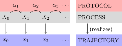
Figure 1: Interaction between the stochastic process $X_{0:N}$, protocol $\alpha_{0:N}$, and realized (observed) trajectories $x_{0:N}$.

We place the following constraints on the SUS.

1. Each system parameter $\alpha_{i}$ leads to a stationary and ergodic stochastic process, realized by holding the protocol fixed indefinitely at $\alpha_{i}$. This implies a unique would-be steady-state distribution $\bm{\pi}_{\alpha_{i}}$ associated to each $\alpha_{i}$.

2. The state and protocol spaces are of even parity, in the sense that we do not negate their values under time reversal, defined precisely later. Sec. II.3 discusses removing this assumption.

We emphasize these are all that is required for the main theoretical result and for meaningful definitions of the excess and housekeeping functionals. Importantly, we do not require dynamics of any particular form or possessing any particular structure—Markovian, Langevin, detailed-balanced, Hamiltonian, master equation, coupled to ideal baths, and so on—beyond that specified by the two conditions above. We do not require states to be microscopic; they can correspond to arbitrary or unknown coarse grainings. With this in mind, even the discrete succession of events is flexible. In particular, from any continuous-time dynamic we may generate a corresponding discrete-time one for appropriately small time steps.

While one cannot, in this most general setting, determine energetics, the fluctuation theorems introduced hold independently and exactly—and at any level of system description. We state the fluctuation theorems in this setting for two primary reasons: first, for clarity of derivation; second, with an eye toward future applications beyond thermodynamic systems to generally nonstationary stochastic processes.

II.1 The thermodynamic system

That said, generality can hinder ease of application. To this end, when presenting the theoretical tools we frequently return to the relevant example “thermal system” of Fig. 2. This is a SUS coupled to an ideal heat bath at inverse temperature $\beta=1/k_{\textnormal{B}}T$, an ideal work reservoir parameterized by $\alpha$, and an auxiliary reservoir representing the otherwise unaccounted-for degrees of freedom. Furthermore, we assign to each SUS state $x$ an energy $E_{\alpha}\pqty{x}$. Finally, while the example system does not assume (order-$1$) Markov dynamics, it does assume no dynamical dependency on times before $t_{0}$. That is, the system’s initial preparation is sufficient to determine the stochastic dynamics during the protocol.

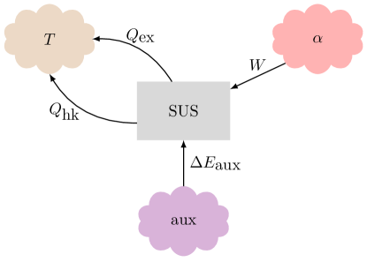
Figure 2: A thermal system and its interactions with various baths. While heat and work reservoirs (labeled with temperature $T$ and parameter $\alpha$, respectively) are ideal, by design we assume nothing about the auxiliary or “aux” reservoir, and so label its energetic contribution by $\Delta E_{\textnormal{aux}}$ to avoid confusion with well-defined terms like heat and work. The labels and arrow directions indicate energetic fluxes to-from the system. Notably, we allow for nonequilibrium steady states and functionally split the total heat $Q$ into the excess heat $Q_{\textnormal{ex}}$—corresponding to adaptive dissipation—and housekeeping heat $Q_{\textnormal{hk}}$—referring to homeostatic dissipation.

These additional restrictions allow identifying the energies associated to each dynamical functional—introduced shortly. While these constraints are minimal, they still allow the SUS to be a coarse-grained representation. In general, this implies that the energetic fluxes are bounds rather than strict equalities espositoStochasticThermodynamicsCoarse2012 .

Of paramount importance—and missing from most idealized thermal schemes—is the presence of the auxiliary bath. The heat and work reservoirs are each proxies for distinct kinds of coarse-grained degrees of freedom with distinct internal structures: the heat reservoir is an infinitely large source of purely thermal energy; the work reservoir is an entropyless source of energy, whose role is to set the SUS’s energetic landscape via parameters $\alpha$.

In contrast, there are no restrictions on the auxiliary reservoir’s structure. It is unnecessary when describing the SUS’s effective state (or energy) at any particular time. Partly, the auxiliary reservoir stands in for coarse-graining out unknown degrees of freedom by unknown schemes. In the case of Rayleigh-Bénard convection, the auxiliary reservoir is a heat bath at a different temperature $T_{2}$. To take another example, in an information ratchet scheme, the auxiliary reservoir may represent the information tape interacting with the ratchet system boydIdentifyingFunctionalThermodynamics2016 ; boydThermodynamicsModularityStructural2018 ; jurgensFunctionalThermodynamicsMaxwellian2020 .

Yet the relevance of the auxiliary bath goes beyond this: specifically, Sec. II.3 shows that it is a necessary source for maintaining NESS conditions in this idealized picture.

Altogether, Fig. 2 captures a large class of mesoscopic physical, chemical, biological, and engineered systems that exhibit nonequilibrium steady states, but that have additional structure and are in contact with at least one thermal environment. We note an important distinction: the “heats” to which we refer in the thermal system context are always associated to the heat bath defined in Fig. 2, and “works” associated to $\alpha$. We avoid calling any fluxes between the auxiliary bath and the system heat or work, since we place no a priori restriction on its structure.

Subsequent sections develop tools for calculating the associated heats and works and for bounding their nonequilibrium fluctuations. Practically, this suggests experimental calorimetry and introduces a valuable way to calibrate effective models—such as, for example, those of the ion channels we take up later.

II.2 Excess energetics

For an ESS system in contact with a single heat bath, the familiar First Law defines work $W$ and heat $Q$ as distinct contributions to its energy change over the course of a protocol jarzynskiNonequilibriumEqualityFree1997 :

$$\Delta E =\underbrace{\int\partial_{\alpha}E_{\alpha}\pqty{x}\differential{\alpha}} +\underbrace{\int\partial_{x}E_{\alpha}\pqty{x}\differential{x}}$$

$$\stackrel{{\scriptstyle.}}{{=}}\qquad\;\;W \qquad\;\;-Q\textnormal{.}$$ (2)

That is, $W$ denotes a difference in system energy owing to a change in protocol—a change in the overall energy landscape—and $Q$ denotes the difference owing to a change in system state—a dissipative signature of its adaptation to environmental conditions.

In contrast, the general setting may not provide a meaningful notion of energy. Worse, even in the restricted case of Fig. 2, we can no longer define total heat for a NESS system by Eq. (2): it leads to contradiction.

To see this, consider a fixed protocol at $\alpha$ and a system poised already in the distribution $\bm{\pi}_{\alpha}$. By definition then $W=0$ and so $\expectationvalue{W}=0$, where $\expectationvalue{\cdot}$ denotes a weighted average over all possible paths. We also have $\expectationvalue{\Delta E}=\Delta\innerproduct{\pi_{\alpha}}{E_{\alpha}}=0$, where:

$$\innerproduct{\pi_{\alpha}}{E_{\alpha}} \stackrel{{\scriptstyle.}}{{=}}\int_{x\in\mathcal{X}}\pi_{\alpha}\pqty{x}E_{\alpha}\pqty{x}\textnormal{.}$$ (3)

Yet we cannot have $\expectationvalue{Q}=0$, for by Eq. (1):

$$\expectationvalue{Q} =\expectationvalue{Q_{\textnormal{hk}}}$$

$$\neq 0~{},$$ (4)

since this is a NESS system. In other words, the observed housekeeping flux, leaving no signature in the state energies, must come from somewhere outside of the system coupled to single ideal heat and work reservoirs. This is precisely what the auxiliary bath provides: in this case $\Delta E_{\textnormal{aux}}=Q_{\textnormal{hk}}$.

However, there is an alternative to energy. Since to every parameter $\alpha$ is an associated steady-state distribution $\bm{\pi}_{\alpha}$, we can define the steady-state surprisal:

$$\phi_{\alpha}\pqty{x}\stackrel{{\scriptstyle.}}{{=}}-\ln\pi_{\alpha}\pqty{x}~{};$$ (5)

so called since it is the Shannon self-information coverElementsInformationTheory2006 of observing state $x$ under the distribution $\bm{\pi}_{\alpha}$.

Taking the surprisal’s state average under this distribution yields its Shannon entropy (or, for continuous-state spaces, its differential entropy):

$$\innerproduct{\pi_{\alpha}}{\phi_{\alpha}} \stackrel{{\scriptstyle.}}{{=}}\int_{x\in\mathcal{X}}\pi_{\alpha}\pqty{x}\phi_{\alpha}\pqty{x}$$

$$=H\bqty{\bm{\pi}_{\alpha}}~{}.$$ (6)

To see how the surprisal relates to energy, consider the canonical ensemble of statistical mechanics—the ESS version of Fig. 2, with $Q_{\textnormal{hk}}=0$ and so no auxiliary bath—where $\bm{\pi}_{\alpha}$ is the Boltzmann distribution sethnaEntropyOrderParameters2021 . Then:

$$-\ln\pi_{\alpha}\pqty{x} =\beta\pqty{E_{\alpha}\pqty{x}-F_{\alpha}^{\textnormal{eq}}}$$

$$=\phi_{\alpha}\pqty{x}~{},$$ (7)

where $F_{\alpha}^{\textnormal{eq}}$ is the equilibrium free energy (the familiar logarithm of the canonical partition function).

Eq. (7) motivates yet another moniker for $\phi_{\alpha}\pqty{x}$: the nonequilibrium potential. In this sense, steady-state surprisal is analogous to a generalized energy. However, it remains a meaningful characterization of a system’s steady-state distribution—via its information-theoretic interpretation—even when energy is not meaningful.

Leveraging this, an analogous First Law for $\phi_{\alpha}\pqty{x}$ defines the excess heat and work:

$$\Delta\phi =\underbrace{\int\partial_{\alpha}\phi_{\alpha}\pqty{x}\differential{\alpha}} +\underbrace{\int\partial_{x}\phi_{\alpha}\pqty{x}\differential{x}}$$

$$\stackrel{{\scriptstyle.}}{{=}}\quad\quad\;\;\mathcal{W}_{\textnormal{ex}} \qquad\;\,-\mathcal{Q}_{\textnormal{ex}}\textnormal{.}$$ (8)

As with their nonexcess counterparts, these quantities characterize distinct dynamical contributions to a change in steady-state surprisal: $\mathcal{W}_{\textnormal{ex}}$ capturing that due to a changing protocol, which sets the steady-state probability landscape; $\mathcal{Q}_{\textnormal{ex}}$ monitoring a system’s adaptation to its environment.

For Fig. 2’s thermal system, these conveniently convert to energies: $\mathcal{W}_{\textnormal{ex}}\to\beta W_{\textnormal{ex}}$ and $\mathcal{Q}_{\textnormal{ex}}\to\beta Q_{\textnormal{ex}}$. And, they agree with other standard formulations of excess thermodynamic functionals hatanoSteadyStateThermodynamicsLangevin2001 ; riechersFluctuationsWhenDriving2017 . Using Eq. (7) and taking the ESS limit of Boltzmann-distributed steady-states yields: (i) $\mathcal{Q}_{\textnormal{ex}}\to\beta Q$—with equilibrium steady states, all dissipated heat is excess—and (ii) $\mathcal{W}_{\textnormal{ex}}\to\beta\pqty{W-\Delta F}$, leading to its classification as an excess environmental entropy production riechersFluctuationsWhenDriving2017 .

We stress, though, that the excess work and heat—and the steady-state surprisal—retain dynamical meaning independent of Boltzmann or even energetic assumptions. In this way, Eq. (7) is a guidepost for thermodynamic interpretation. It is not, however, a strict equivalence. In point of fact, as we will see, sodium channels (as with other NESS systems) lack a well-defined steady-state free energy riechersFluctuationsWhenDriving2017 . Nevertheless, Eq. (8) describes—tractably—two functionally distinct aspects of their response to dynamic environments.

II.3 Detailed balance and housekeeping

The housekeeping heat remains. Recall that it corresponds to energy dissipated to maintain NESSs, as in Eq. (1). Phenomenologically, Eq. (1) provided a satisfactory answer. However, our excess heat definition only required would-be steady-state distributions exist. The definition of total heat, in contrast, depended explicitly on well-defined state energies. This difference led to problems with NESSs.

The upshot is that a more general definition of housekeeping heat is called for. In particular, it should depend only on the stochastic dynamics and, when added to excess heat, it should give a reasonable generalization of total heat. Naturally, we also require interpretability and that it reduces to the corresponding well-understood thermodynamic terms in the appropriate limits.

To these ends, but in a slightly more general form than previously reported, we define housekeeping heat to explicitly allow non-Markovian dynamics:

$$\mathcal{Q}_{\textnormal{hk}}\stackrel{{\scriptstyle.}}{{=}}\ln\, \frac{\mathrm{Pr}\left(X_{1:N}=x_{1:N\phantom{-1}}~{}\middle|~{}X_{0}=x_{0\phantom{N}};\alpha_{0:N}\right)}{\mathrm{Pr}\left(X_{1:N}=x_{N-1:0}~{}\middle|~{}X_{0}=x_{N\phantom{0}};\alpha_{N:0}\right)}$$

$$+\ln\prod_{i=0}^{N-1}\frac{\pi_{\alpha_{i+1}}\pqty{{}_{\phantom{+}}x_{i\phantom{1}}}}{\pi_{\alpha_{i+1}}\pqty{x_{i+1}}}\textnormal{.}$$ (9)

Observe that the first term is a log-ratio of conditioned path probabilities. The denominator is the numerator’s time reversal: the probability of obtaining the reversed path $x_{N:0}$ conditioned on starting in the state $x_{N}$ and subject to the reversed protocol $\alpha_{N:0}$. The second term is exactly $-\mathcal{Q}_{\textnormal{ex}}$ by the discrete form of Eq. (8). And so, by identifying $\mathcal{Q}\stackrel{{\scriptstyle.}}{{=}}\mathcal{Q}_{\textnormal{ex}}+\mathcal{Q}_{\textnormal{hk}}$, housekeeping heat is a component of the generalized total heat $\mathcal{Q}$.

In the (single heat bath) thermal example, one recovers units of energy as $\mathcal{Q}\to\beta Q$ and $\mathcal{Q}_{\textnormal{hk}}\to\beta Q_{\textnormal{hk}}$. And, the resulting total heat is consistent with formulations based on microscopic reversibility crooksEntropyProductionFluctuation1999 . Equivalently, we could have started with this microscopic reversibility condition for even state spaces and arrived at the appropriate housekeeping heat.

With this in mind, consider relaxing the even state space assumption. Doing so and keeping the appropriate microscopic reversibility condition allows for an analogous splitting of housekeeping heat—modified so that the denominator’s terms are negated where required—and excess heat, consistent with previous considerations of odd-parity NESS systems spinneyNonequilibriumThermodynamicsStochastic2012 ; yeoHousekeepingEntropyContinuous2016 . While we note that an analogue to our Eq. (24) holds, we do not treat this further here.

Now, consider a Markov dynamic of order $1$. That is, conditioning on the previous time step fully characterizes the probability distribution over futures. Then, the first term reduces to the logarithm of a product of one-step conditional probabilities. And, $\mathcal{Q}_{\textnormal{hk}}$ tracks the degree of detailed-balance violation over the trajectory. This is in agreement with existing definitions hatanoSteadyStateThermodynamicsLangevin2001 ; harrisFluctuationTheoremsStochastic2007 ; riechersFluctuationsWhenDriving2017 . Concretely, detailed-balanced dynamics imply $\mathcal{Q}_{\textnormal{hk}}=0$ for every trajectory. If any trajectory yields $\mathcal{Q}_{\textnormal{hk}}\neq 0$, the dynamic is necessarily nondetailed-balanced.

Finally, recall that by definition $\mathcal{Q}_{\textnormal{hk}}=0$ for an ESS system. Taken together with assuming an even state space—ensuring correct “reverse” probabilities—the Markov condition says, succinctly:

nondetailed-balanced dynamics

$$\qquad\Updownarrow$$

nonequilibrium steady states.

Recall that the Markov condition is appropriate for many microscopically-modeled thermal systems such as overdamped Langevin dynamics, as well as for a host of biological systems like the ion channels we consider later.

Nonzero housekeeping heat actually necessitates including an auxiliary reservoir for a complete picture. Recall Fig. 2. This follows since a NESS system, even fully relaxed to its stationary distribution, constantly dissipates housekeeping heat to the thermal reservoir. (And does so at an average rate of $\differential\expectationvalue{Q_{\textnormal{hk}}}/\differential t$.) Yet, with the protocol parameter fixed, no work (or excess work) is done: $W=0$ by Eq. (2). The system’s average energy does not change, though, since the parameter and individual state uniquely set its energies: $\differential\expectationvalue{E}/\differential t=0$.

The conclusion is that energy flux through the system, observed in the housekeeping dissipation to the thermal reservoir, must come from somewhere not otherwise described by the ideal constructs. In other words, in the thermodynamically-interpretable setting, nondetailed-balanced dynamics are signatures of unaccounted-for degrees of freedom. In this way, the constructions in Eqs. (8) and (9) provide the tools to isolate this homeostatic part of a system’s energetic fluxes, so called for its role maintaining homeostatic (steady-state) conditions.

We close by calling out a feature on direct display in Eq. (9). While placing minimal restrictions on the dynamics, problems arise when any path is strictly irreversible, in the sense that a nonzero-probability forward trajectory is associated a zero-probability reverse. Then, $\mathcal{Q}_{\textnormal{hk}}$ diverges. And this seemingly forbids dynamics in finite state spaces with one-way-only transitions.

In the thermodynamic interpretation, such a transition costs infinite dissipation. And, with this realization, usually a model’s mesoscopic nature comes to bear. Indeed, Ref. riechersFluctuationsWhenDriving2017 in its related sodium channel analysis remarks that “more careful experimental effort should be done to bound the actual housekeeping entropy production in these ion channels”. The following section demonstrates that a new trajectory class fluctuation theorem provides a tool for analyzing such experiments and circumvents the divergence while still placing strong bounds on fluctuations.

III Fluctuations and Free Energy

So far, we defined the generalized quantities $\mathcal{W}_{\textnormal{ex}}$, $\mathcal{Q}_{\textnormal{ex}}$, and $\mathcal{Q}_{\textnormal{hk}}$ and elucidated their meanings outside the ESS regime. As with their ESS counterparts, though, they depend on the specific path a system takes through its state space under a particular protocol. A suite of statistical tools called fluctuation theorems (FTs) tie such nonequilibrium behaviors to equilibrium (or steady-state, more generally) quantities. They come in three primary flavors: (i) integral FTs (IFTs) concern weighted averages over all possible trajectories, (ii) detailed FTs (DFTs) fix the relationship between a specific path and its associated reversal, and (iii) trajectory class FTs (TCFTs) interpolate between the two Wims19a .

The remainder of this section compares and contrasts these, discusses their relation to free energy, and concludes with a TCFT for NESS systems. This sets the stage for analyzing the two ion channels’ thermodynamic responses—expressed in terms of excess work, excess heat, and housekeeping heat—to complex environmental signals.

III.1 Fluctuation theorems

Integral and detailed FTs each exhibit complementary tradeoffs—tradeoffs discussed below as we introduce the theorems. TCFTs, meanwhile, combine the strengths of both and so are adaptable to a variety of systems and experimental conditions. Here we present a general TCFT valid for NESS systems. It simultaneously extends the previously known ESS FT and reveals experimental difficulties unique to NESS systems, ultimately suggesting a need for new experimental tools.

Jarzynski’s equality jarzynskiEquilibriumFreeenergyDifferences1997 ; jarzynskiNonequilibriumEqualityFree1997 , an IFT and the progenitor of the FTs we consider, links equilibrium free energies to the averaged exponential work distribution. It applies specifically to ESS systems that begin in their equilibrium distribution and are connected to a single heat bath. Under these conditions:

$$\expectationvalue{\mathrm{e}^{-\beta W}}=\mathrm{e}^{-\beta\Delta F^{\textnormal{eq}}}~{},$$ (10)

where the angle brackets again refer to a weighted average over all possible trajectories. That is, Jarzynski’s equality ties an arbitrarily nonequilibrium quantity—the averaged exponential work $\expectationvalue{\mathrm{e}^{-\beta W}}$—to the equilibrium free energy difference $\Delta F^{\textnormal{eq}}$—a state function. Practically, this enables free energy estimation from nonequilibrium work measurements cetinerRecoveryEquilibriumFree2020 .

It comes with disadvantages, however. In particular, extremely rare paths often dominate the exponential work distribution jarzynskiRareEventsConvergence2006 , leading to poor statistical accuracy when estimating with finitely many experimental realizations. Nonetheless, Jarzynski’s equality has been confirmed for a wide variety of systems hummerFreeEnergyReconstruction2001 ; liphardtEquilibriumInformationNonequilibrium2002 ; jarzynskiWorkFluctuationTheorems2006 . In addition, while Eq. (10) only applies to ESS systems, a variety of generalizations have been derived and tested for NESS systems hatanoSteadyStateThermodynamicsLangevin2001 ; trepagnierExperimentalTestHatano2004 ; speckIntegralFluctuationTheorem2005 ; seifertStochasticThermodynamicsFluctuation2012 .

In contrast to Jarzynski’s IFT, the detailed FTs (DFTs), express a symmetry relation between a particular trajectory-protocol pair and its appropriate time reversal. Perhaps the most well-known of these is due to Crooks crooksNonequilibriumMeasurementsFree1998 ; crooksEntropyProductionFluctuation1999 , which is complementary to Jarzynski’s IFT in several ways. For one, it makes the same assumptions: an ESS system connected to a bath, beginning in equilibrium and driven away from it. For another, Jarzynski’s IFT results directly from trajectory-averaging both sides of Crooks’ DFT. Before presenting the DFT, though, we pause to precisely define and set notation for what we mean by an “appropriate reversal”.

Consider a system that begins in state distribution $\bm{\mu}_{\textnormal{F}}$, is driven by the protocol $\alpha_{1:N}$, and realizes a trajectory in the measurable subset $C\subseteq\mathcal{X}^{N+1}$. We call $C$ a trajectory class. Then, we define the forward process probability as:

$$\mathcal{P}_{\bm{\mu}_{\textnormal{F}}}\left(C\right)\stackrel{{\scriptstyle.}}{{=}}\mathrm{Pr}\left(C~{}\middle|~{}X_{0}\sim\bm{\mu}_{\textnormal{F}};\alpha_{1:N}\right)~{}.$$ (11)

(Here, $\sim$ means “is distributed as”.) Now, consider the same system beginning in the distribution $\bm{\mu}_{\textnormal{R}}$ and driven by the reverse protocol $\widetilde{\alpha}_{N:1}$, where the tilde indicates negation of time-odd variables (such as magnetic field). In turn, we define the reverse process probability:

$$\mathcal{R}_{\bm{\mu}_{\textnormal{R}}}\left(C\right)\stackrel{{\scriptstyle.}}{{=}}\mathrm{Pr}\left(C~{}\middle|~{}X_{0}\sim\bm{\mu}_{\textnormal{R}};\widetilde{\alpha}_{N:1}\right)\textnormal{.}$$ (12)

For finite state spaces, Eqs. (11) and (12) define distinct probability measures on the trajectory space. In a continuous state space, we use the same notation to indicate probability densities.

Let $\bm{\pi}_{\textnormal{F}}\stackrel{{\scriptstyle.}}{{=}}\bm{\pi}_{\alpha_{0}}$ and $\bm{\pi}_{\textnormal{R}}\stackrel{{\scriptstyle.}}{{=}}\bm{\pi}_{\widetilde{\alpha}_{N}}$. In these terms, Crooks’ DFT reads:

$$\frac{\mathcal{P}_{\bm{\pi}_{\textnormal{F}}}\left(x_{0:N}\right)}{\mathcal{R}_{\bm{\pi}_{\textnormal{R}}}\left(\widetilde{x}_{N:0}\right)}=\mathrm{e}^{\beta\pqty{W-\Delta F^{\textnormal{eq}}}}\textnormal{.}$$ (13)

As with Jarzynski’s IFT, the Crooks DFT has withstood experimental test collinVerificationCrooksFluctuation2005 and seen use in empirically estimating free energy differences cetinerRecoveryEquilibriumFree2020 . Also, paralleling Jarzynski’s IFT, Crooks’ DFT has been generalized to a variety of NESS systems lahiriFluctuationTheoremsExcess2014 ; mandalEntropyProductionFluctuation2017 ; riechersFluctuationsWhenDriving2017 .

We highlight Ref. riechersFluctuationsWhenDriving2017 ’s generalization of these. We recall, in particular, its Eq. (25), since it is the DFT upon which we base our TCFT.

Here and in the remainder, we assume even state and protocol spaces (keeping in mind Sec. II.3’s notes on relaxing this assumption), so there is never negation under time reversal. However, in further contrast to Crooks’ DFT, we do not assume equilibrium steady states (or detailed balance), any particular starting distribution for the forward and reverse processes, nor a single heat bath system (or any specific bath structure). Instead, we require only the functionals $\mathcal{W}_{\textnormal{ex}}$ and $\mathcal{Q}_{\textnormal{hk}}$ as defined in Eqs. (8) and (9), along with an additional one—the (unitless) nonsteady-state free energy:

$$\mathcal{F}^{\textnormal{nss}}_{\alpha}\pqty{\bm{\mu},x} \stackrel{{\scriptstyle.}}{{=}}\ln\frac{\mu\pqty{x}}{\pi_{\alpha}\pqty{x}}~{}.$$ (14)

Its name derives from its indicating how far a given distribution is from the associated steady-state distribution. Indeed, on state averaging we have $\innerproduct{\mu}{\mathcal{F}^{\textnormal{nss}}_{\alpha}}=D_{\textnormal{KL}}\bqty{\bm{\mu}\,\|\,\bm{\pi}_{\alpha}}$, where $D_{\textnormal{KL}}\bqty{\bm{p}\,\|\,\bm{q}}$ is the Kullback-Leibler divergence between distributions $p$ and $q$ Cove06a . As with the other functionals generalized to the stochastic process picture, it carries meaning—departure from steady-state conditions
—outside of energetic or thermal assumptions.

Given this, Ref. riechersFluctuationsWhenDriving2017 ’s DFT is:

$$\frac{\mathcal{R}_{\bm{\mu}_{\textnormal{R}}}\left(x_{N:0}\right)}{\mathcal{P}_{\bm{\mu}_{\textnormal{F}}}\left(x_{0:N}\right)}=\mathrm{e}^{-\pqty{\mathcal{W}_{\textnormal{ex}}+\mathcal{Q}_{\textnormal{hk}}-\Delta\mathcal{F}^{\textnormal{nss}}}}~{},$$ (15)

where $\Delta\mathcal{F}^{\textnormal{nss}}=\mathcal{F}^{\textnormal{nss}}_{\alpha_{N}}\pqty{\bm{\mu}_{\textnormal{R}},x_{N}}-\mathcal{F}^{\textnormal{nss}}_{\alpha_{0}}\pqty{\bm{\mu}_{\textnormal{F}},x_{0}}$ is a correction due to starting the forward and reverse processes out of steady state. If we began the forward and reverse processes in their associated steady-state distributions, by definition we would have $\Delta\mathcal{F}^{\textnormal{nss}}=0$.

As a mathematical statement involving a stochastic process’ trajectories, their probabilities, and the functionals $\mathcal{W}_{\textnormal{ex}}$, $\mathcal{Q}_{\textnormal{hk}}$, and $\Delta\mathcal{F}^{\textnormal{nss}}$ we have so far defined, Eq. (15) holds independent of any thermodynamic assumptions. Yet, as before, reducing it to thermodynamically meaningful cases is straightforward and illuminates several important considerations when moving from ESS into NESS regimes.

III.2 Multiple NESS IFTs and second laws

In the ESS case, Eq. (15) reduces neatly to Crooks’ DFT of Eq. (13), which under integration directly yields Jarzynski’s equality. However, the NESS setting introduces more freedom under this type of integration.

Consider rearranging Eq. (15) like so:

$$\mathcal{R}_{\bm{\mu}_{\textnormal{R}}}\left(x_{N:0}\right)=\mathcal{P}_{\bm{\mu}_{\textnormal{F}}}\left(x_{0:N}\right)\mathrm{e}^{-\pqty{\mathcal{W}_{\textnormal{ex}}+\mathcal{Q}_{\textnormal{hk}}-\Delta\mathcal{F}^{\textnormal{nss}}}}\textnormal{.}$$ (16)

Then integrate both sides over all trajectories $x_{0:N}$. The righthand side directly yields the forward trajectory average of the exponential, while the lefthand side yields $1$ by probability conservation (and since the sets of all measurable forward and reverse trajectories are the same set). This gives a generalized IFT:

$$1=\expectationvalue{\mathrm{e}^{-\pqty{\mathcal{W}_{\textnormal{ex}}+\mathcal{Q}_{\textnormal{hk}}-\Delta\mathcal{F}^{\textnormal{nss}}}}}$$ (17)

and—via Jensen’s inequality—a generalized second law:

$$\expectationvalue{\mathcal{W}_{\textnormal{ex}}}+\expectationvalue{\mathcal{Q}_{\textnormal{hk}}}-\Delta D_{\textnormal{KL}}\bqty{\bm{\mu}\,\|\,\bm{\pi}}\geq 0\textnormal{,}$$ (18)

where $\Delta D_{\textnormal{KL}}\bqty{\bm{\mu}\,\|\,\bm{\pi}}=D_{\textnormal{KL}}\bqty{\bm{\mu}_{\textnormal{R}}\,\|\,\bm{\pi}_{\textnormal{R}}}-D_{\textnormal{KL}}\bqty{\bm{\mu}_{\textnormal{F}}\,\|\,\bm{\pi}_{\textnormal{F}}}$. This latter term is a classical analogue to the “initial-state dependence” of Ref. riechersInitialstateDependenceThermodynamic2021 ; it quantifies additional entropic dissipation when beginning and ending out of the steady-state distribution.

Yet Eq. (17) is not unique. To take one example, by direct calculation as in Ref. hatanoSteadyStateThermodynamicsLangevin2001 , we find for Markov dynamics:

$$1=\expectationvalue{\mathrm{e}^{-\mathcal{F}^{\textnormal{nss}}_{\alpha_{0}}\pqty{\bm{\mu}_{\textnormal{F}},\,x_{0}}-\mathcal{W}_{\textnormal{ex}}}}$$ (19)

$$\implies\expectationvalue{\mathcal{W}_{\textnormal{ex}}}+D_{\textnormal{KL}}\bqty{\bm{\mu}_{\textnormal{F}}\,\|\,\bm{\pi}_{\textnormal{F}}}\geq 0\textnormal{,}$$ (20)

a slight generalization of their result with the inclusion of initial-state dependence (thereby relaxing the requirement of steady-state initial conditions). In other words, a second law holds for $\expectationvalue{\mathcal{W}_{\textnormal{ex}}}$ itself, not just for its sum with $\expectationvalue{\mathcal{Q}_{\textnormal{hk}}}$. This is not only a meaningfully different bound, but this IFT also does not result naturally from the underlying DFT.

To take another example, directly substituting $\expectationvalue{\mathcal{Q}_{\textnormal{hk}}}=\expectationvalue{\mathcal{Q}}-\expectationvalue{\mathcal{Q}_{\textnormal{ex}}}$ into Eq. (17) generalizes to a different IFT:

$$1=\expectationvalue{\mathrm{e}^{-\pqty{\mathcal{Q}+\Delta\phi-\Delta\mathcal{F}^{\textnormal{nss}}}}}\textnormal{,}$$ (21)

first proven in Ref. speckIntegralFluctuationTheorem2005 .

Finally, taken on their own, Eqs. (18) and (20) do not imply a third NESS IFT—and so Second Law—for housekeeping heat alone; cf. again Ref. speckIntegralFluctuationTheorem2005 . However, as we now show, it is implied rather directly by the combination of Eqs. (15) and (19).

First rearrange Eq. (15) as:

$$\mathcal{R}_{\bm{\mu}_{\textnormal{R}}}\left(x_{N:0}\right)\mathrm{e}^{\mathcal{W}_{\textnormal{ex}}-\mathcal{F}^{\textnormal{nss}}_{\alpha_{N}}\pqty{\bm{\mu}_{\textnormal{R}},x_{N}}}$$

$$\qquad=\mathcal{P}_{\bm{\mu}_{\textnormal{F}}}\left(x_{0:N}\right)\mathrm{e}^{-\mathcal{Q}_{\textnormal{hk}}-\mathcal{F}^{\textnormal{nss}}_{\alpha_{0}}\pqty{\bm{\mu}_{\textnormal{F}},x_{0}}}~{}.$$

Again, we wish to integrate both sides over all $x_{0:N}$, but at first glance the lefthand side (first line) poses an issue: $\mathcal{W}_{\textnormal{ex}}$ refers to the excess work over a trajectory driven by the forward protocol, while $\mathcal{R}$ is the probability of a trajectory as driven by the reverse protocol.

Fortunately, $\mathcal{W}_{\textnormal{ex}}$ is odd under full time reversal: $\mathcal{W}_{\textnormal{ex}}=-\mathcal{W}_{\textnormal{ex}}^{\textnormal{R}}$, where $\mathcal{W}_{\textnormal{ex}}^{\textnormal{R}}$ is the excess work generated by the time-reversed trajectory driven by the time-reversed protocol. This matches up driving protocols and “initial” conditions on the lefthand side. Since Eq. (19) holds regardless of the chosen protocol or starting distribution, under integration the lefthand side is unity. The righthand side, meanwhile, becomes simply the forward trajectory average of its argument. And, we obtain the generalized IFT for housekeeping heat:

$$1=\expectationvalue{\mathrm{e}^{-\mathcal{F}^{\textnormal{nss}}_{\alpha_{0}}\pqty{\mu_{\textnormal{F}},\,x_{0}}-\mathcal{Q}_{\textnormal{hk}}}}$$ (22)

$$\implies\expectationvalue{\mathcal{Q}_{\textnormal{hk}}}+D_{\textnormal{KL}}\bqty{\bm{\mu}_{\textnormal{F}}\,\|\,\bm{\pi}_{\textnormal{F}}}\geq 0\textnormal{,}$$ (23)

once again extended to include the effects of initial-state dependence.

To adopt Ref. speckIntegralFluctuationTheorem2005 ’s language, these IFTs—for $\mathcal{W}_{\textnormal{ex}}+\mathcal{Q}_{\textnormal{hk}}$, $\mathcal{W}_{\textnormal{ex}}$-only, $\mathcal{Q}+\Delta\phi$, and $\mathcal{Q}_{\textnormal{hk}}$-only—are “genuinely different” but no longer require especially “different derivation[s]” nor restrictive physical assumptions. To emphasize the former point, though: just as with the equilibrium second law $\expectationvalue{\Delta S}\geq 0$, these hold only under full trajectory averaging. That is, individual rare trajectories (or sets thereof) may well produce negative excess works, negative housekeeping heats, or both. Sec. V.1 explores these consequences for our example ion channels.

Notably absent is the notion of steady-state free energy, analogous to the equilibrium free energy from Jarzynski’s equality. Defining one for general NESS systems remains problematic, in part since the steady-state distributions may no longer be Boltzmann. Instead, the excess work subsumes what would have been a steady-state free energy difference, and we work directly with it. The downside, however, is the inability to extract such a free energy as a “steady state” quantity separate from the path-dependent nonequilibrium dynamical ones. Indeed, this was an extremely important consequence of Eq. (10).

The suite of IFTs given by our Eqs. (18), (20), and (23), however, do include strong connections between path-independent and path-dependent quantities in the form of initial-state dependence and changes in steady-state surprisal. Unlike for ESS systems, however, even in well-controlled NESS thermal examples applying the IFTs presents a rather serious experimental challenge: direct measurement of heat (most notably housekeeping heat). Even when testing FTs phrased in terms of heat, often work (excess or not) is experimentally tracked trepagnierExperimentalTestHatano2004 . And so, we expect direct measurement to be a key, requisite step in leveraging the resulting FTs to analyze experimental NESS systems.

III.3 NESS trajectory class fluctuation theorem

With appropriate DFTs and IFTs for NESS systems now in hand, we are confronted with yet another challenging experimental tradeoff. Just as the IFTs suffer from extremely rare-but-large contributions, the DFTs require precise control and measurement of individual realizations, as well as accurate estimations of individual realization probabilities (or their ratios). This is often intractable even in principle. For example, as experimental systems, the ion channels considered shortly do not permit measurement of the conformational states themselves. Instead, ionic current is the only observable. Moreover, the state space topology varies with each individual rate model vandenbergSodiumChannelGating1991 . This is all to say that thermodynamic analysis requires a more flexible intermediary between the DFT’s trajectory-level information and the IFT’s ensemble-level information.

Ref. Wims19a recently provided just such an intermediary for ESS systems—the trajectory class FT (TCFT). At root, it relates the forward and reverse probabilities of an arbitrary subset of trajectories—the trajectory class $C$ as introduced earlier—to the average exponential work within that trajectory class. In this way, the TCFT is maximally adaptable to experimental conditions: It need neither suffer rare-event errors nor require individual-trajectory-level control. Instead, whatever the unique experimental conditions at hand, it provides a framework for laying out an associated FT. As a practical matter, the TCFT has already provided a diagnostic tool for monitoring the thermodynamics of successful and failed microscopic information processing in superconducting flux logic Wims19a ; sairaNonequilibriumThermodynamicsErasure2020 .

The following extends Ref. Wims19a ’s ESS TCFT (Eq. (3) there) in two ways. First, we allow for NESS systems. Second, we allow starting the forward and reverse processes in arbitrary distributions $\bm{\mu}_{\textnormal{F}}$ and $\bm{\mu}_{\textnormal{R}}$, respectively. This results in our exponential NESS TCFT, derived in App. A:

$$\frac{\mathcal{R}_{\bm{\mu}_{\textnormal{R}}}\left(C_{\textnormal{R}}\right)}{\mathcal{P}_{\bm{\mu}_{\textnormal{F}}}\left(C\right)}=\expectationvalue{\mathrm{e}^{-\pqty{\mathcal{W}_{\textnormal{ex}}+\mathcal{Q}_{\textnormal{hk}}-\Delta\mathcal{F}^{\textnormal{nss}}}}}_{C}~{},$$ (24)

where $\expectationvalue{\cdot}_{C}$ denotes the conditionally-weighted average over only those trajectories in the class $C$ and the reverse trajectory class $C_{\textnormal{R}}\stackrel{{\scriptstyle.}}{{=}}\set{x_{N:0}\,}{\,x_{0:N}\in C}$.

Eq. (24) imports to the NESS setting all the benefits of the TCFT. Most notably, it adapts readily to a variety of experimental conditions while maintaining robust statistics. The associated DFT and IFT emerge simply by setting the class $C$ to be a single trajectory or the set of all trajectories, respectively. Equation (24), as with its ESS counterpart, allows selecting trajectory classes most accessible in a particular experimental configuration and then proposes the appropriate theory against which to test.

Once again, in this form Eq. (24) makes only two assumptions about a stochastic process, as outlined previously: a unique stationary distribution for each $\alpha$ and an even state space. It reproduces Ref. Wims19a ’s TCFT given ESS assumptions. Similarly, it reproduces Ref. riechersFluctuationsWhenDriving2017 ’s Eq. (52) when the class is chosen to start and end in a particular desired subset of states. However, our main result holds independently of any energetic, Markovian, or particular class assumption.

Generalization to NESS systems is not without caveat, however. $\mathcal{Q}_{\textnormal{hk}}$ plays a central role and we do not have our state- and path-independent equilibrium free energy to extract from the average and estimate. This suggests experimentally tracking the housekeeping heat itself is key to understanding nondetailed balanced, NESS systems. (Alternatively, one could monitor the total heat per Eq. (18).) This is not surprising, considering $Q_{\textnormal{hk}}$ is the defining difference between an ESS and NESS system.

IV Na⁺ and K⁺ Ion Channels

Armed with this toolkit, we are now ready to probe the thermodynamic functionality of two example biophysical systems: Ref. dayanTheoreticalNeuroscienceComputational2001 ’s delayed-rectifier potassium (K⁺) and fast sodium (Na⁺) voltage-gated ion channels. (See its Figs. 5.12 and 5.13, reproduced in our Figs. 3 and 4, respectively.) These single-channel models are based on relatively more macroscopic descriptions of channel ensembles due to Hodgkin and Huxley hodgkinQuantitativeDescriptionMembrane1952 . However, they better represent the interdependencies between molecular-conformational transformations and more accurately reproduce experimentally-observed currents, especially for the Na⁺ channel dayanTheoreticalNeuroscienceComputational2001 .

The models are both continuous-time Markov chains (CTMCs), whose dynamics are described by the stochastic master equation:

$$\derivative{t}\bra{\mu\pqty{t}}=\bra{\mu\pqty{t}}\mathbf{\mathbf{G}}_{\alpha}\textnormal{.}$$ (25)

The row vector $\bra{\mu\pqty{t}}$ specifies the state distribution or mixed state at time $t$; its elements are $\mu\pqty{x,t}\stackrel{{\scriptstyle.}}{{=}}\mathrm{Pr}\left(X\pqty{t}=x\right)$. The transition rate matrix $\mathbf{\mathbf{G}}_{\alpha}$ is controlled by the protocol and, thus, varies with time. The would-be steady-state distributions for each $\alpha$ are given by:

$$\bra{\pi_{\alpha}}\mathbf{G}_{\alpha}=\bra{0}~{},$$ (26)

with $\bra{0}$ the all-$0$ vector.

The transition-rate matrices corresponding to the two channels are:

$$\mathbf{G}_{\alpha}^{\textnormal{K${}^{+}$\phantom{a}}} =\begin{bmatrix}-4a_{n}&4a_{n}&0&0&0\\ b_{n}&-\pqty{3a_{n}+b_{n}}\phantom{+k_{1}}&3a_{n}&0&0\\ 0&2b_{n}&-\pqty{2a_{n}+2b_{n}}\phantom{+k_{2}}&2a_{n}&0\\ 0&0&3b_{n}&-\pqty{3b_{n}+a_{n}}\phantom{+k_{3}}&a_{n}\\ 0&0&0&4b_{n}&-4b_{n}\end{bmatrix}\textnormal{ and}$$ (27)

$$\mathbf{G}_{\alpha}^{\textnormal{Na${}^{+}$}} =\begin{bmatrix}-3a_{m}&3a_{m}&0&0&0\\ b_{m}&-\pqty{2a_{m}+b_{m}+k_{1}}&2a_{m}&0&k_{1}\\ 0&2b_{m}&-\pqty{a_{m}+2b_{m}+k_{2}}&a_{m}&k_{2}\\ 0&0&3b_{m}&-\pqty{3b_{m}+k_{3}}&k_{3}\\ 0&0&a_{h}&0&-a_{h}\phantom{4}\end{bmatrix}\textnormal{.}$$ (28)

Letting $\alpha$ denote the transmembrane voltage, the associated transition rates are:

$$a_{m}\pqty{\alpha} =\frac{\pqty{\alpha+40\textnormal{ mV}}/10\textnormal{ mV}}{1-\exp\pqty{-\pqty{\alpha+40\textnormal{ mV}}/10\textnormal{ mV}}}\textnormal{,} b_{m}\pqty{\alpha}=4\exp\pqty{-\pqty{\alpha+65\textnormal{ mV}}/18\textnormal{ mV}}\textnormal{,}$$ (29)

$$a_{h}\pqty{\alpha} =\frac{7}{100}\exp\pqty{-\pqty{\alpha+65\textnormal{ mV}}/20\textnormal{ mV}}\textnormal{,} k_{1}=\frac{6}{25}\textnormal{ ms}^{-1}\textnormal{, }k_{2}=\frac{2}{5}\textnormal{ ms}^{-1}\textnormal{, }k_{3}=\frac{3}{2}\textnormal{ ms}^{-1}\textnormal{,}$$ (30)

$$a_{n}\pqty{\alpha} =\frac{\pqty{\alpha+55\textnormal{ mV}}/100\textnormal{ mV}}{1-\exp\pqty{-\pqty{\alpha+55\textnormal{ mV}}/10\textnormal{ mV}}}\textnormal{, and}\qquad b_{n}\pqty{\alpha}=\frac{1}{8}\exp\pqty{-\pqty{\alpha+65\textnormal{ mV}}/80\textnormal{ mV}}\textnormal{.}$$ (31)

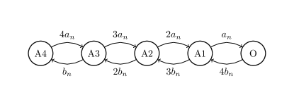
Figure 3: Continuous-time Markov chain model of the K⁺ channel adapted from Fig. 5.12 of Ref. dayanTheoreticalNeuroscienceComputational2001 . Self-transitions are implied. In the states labeled A$n$, a number $n\in\{1,2,3,4\}$ activation gates close the channel. O labels the open channel state, the only one in which K⁺ current can flow through the channel. The rate parameters $a_{n}$ and $b_{n}$ are voltage-dependent; their functional forms are given in Eqs. (31). This channel model is fully detailed-balanced, in the sense that Eq. (33) vanishes for every allowed transition pair.

We map these CTMC systems to discrete-time stochastic processes by taking $\alpha\pqty{t}$ fixed for sufficiently small time intervals $\Delta t$, generating the transition matrices:

$$\mathbf{T}_{\alpha}^{\Delta t}\stackrel{{\scriptstyle.}}{{=}}\mathrm{e}^{\Delta t\,\mathbf{G}_{\alpha}}$$ (32)

for each such time interval. Having discretized time in this way, they are examples of the thermodynamic scheme in Fig. 2, being surrounded by a single thermal environment at body temperature.

A voltage-gated ion channel’s basic function is to selectively allow ions to permeate a cell membrane. The selection is based on the transmembrane voltage—the voltage difference between the membrane’s inside and outside. In our models, this difference is specified by the parameter $\alpha$, and so a neuronal action potential spike is a specific protocol. Ref. dayanTheoreticalNeuroscienceComputational2001 ’s K⁺ and Na⁺ models correspond to channels that play crucial roles in generating and propagating such spikes in mammalian neuronal axons. Both Markov chain models are estimated from single-channel experiments.

We selected these two channel models for several reasons.

First, in terms of their biological function, they are comparable: They accomplish similar tasks, are connected to the same environmental parameters, and are suitably mesoscopic. That is, despite being more detailed than the Hodgkin-Huxley ensemble models, neither model accounts for the many additional molecular degrees of freedom involved in the channel dynamics, be it steady-state or transient functions. The small effective state spaces in the Markov chain models reflect this.

One consequence of this implied coarse graining is that any total entropy production is a lower bound espositoStochasticThermodynamicsCoarse2012 . Still, we are able to make headway analyzing their nonequilibrium dynamics without knowledge of the underlying coarse-graining methods—knowledge missing for the vast majority of mesoscopic complex systems.

Second, the Na⁺ channel’s transition rates do not, in general, satisfy detailed balance, while the K⁺ channel’s do. Indeed, the Na⁺ channel model includes both finitely nondetailed-balanced transition pairs and one-way-only transition rates, which imply divergent infinitesimal-time housekeeping heat. These violations of ideality are typical and widely encountered in molecular biophysical systems, as well as in real-world thermodynamic processes.

To appreciate these nonidealities, note that under our time discretization and the Markov property, the infinitesimal(-time) housekeeping heat—a single “step” of Eq. (9)—for a transition between states indexed by $i$ to $j$:

$$\bqty{\differential\mathcal{Q}_{\textnormal{hk}}}_{ij} =\lim_{\Delta t\to 0}\ln\frac{\pi_{\alpha}\pqty{x_{i}}\bqty{\mathbf{T}_{\alpha}^{\Delta t}}_{ij}}{\pi_{\alpha}\pqty{x_{j}}\bqty{\mathbf{T}_{\alpha}^{\Delta t}}_{ji}}$$

$$=\lim_{\Delta t\to 0}\ln\frac{\pi_{\alpha}\pqty{x_{i}}\bqty{\mathbf{G}_{\alpha}+\mathcal{O}\pqty{\Delta t}}_{ij}}{\pi_{\alpha}\pqty{x_{j}}\bqty{\mathbf{G}_{\alpha}+\mathcal{O}\pqty{\Delta t}}_{ji}}\textnormal{.}$$ (33)

For systems with one-way-only transition rates, such as from the second to the fifth state of the Na⁺ channel (indexing the states left to right, Fig. 4), infinitesimal housekeeping heat diverges. This contrast between the two channels—wherein one of them exhibits equilibrium steady states and the other nonequilbrium steady states—allows showcasing several features of the NESS TCFT and of the NESS framework more broadly. These, in turn, reveal the dynamical interplay of different modes of thermodynamic transformation.

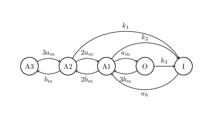
Figure 4: Continuous-time Markov chain model of the Na⁺ channel adapted from Fig. 5.13 of Ref. dayanTheoreticalNeuroscienceComputational2001 . Self-transitions are implied. In the states labeled A$n$, a number $n\in\{1,2,3\}$ activation gates close the channel. O labels the open channel state, in which Na⁺ current flows through the channel. Finally, I labels the channel’s inactivation by its inactivation gate—its so-called ball and chain. The rate parameters $a_{m}$, $b_{m}$, and $a_{h}$ are all voltage-dependent; their functional forms are given in Eqs. (29)–(30). The rate constants $k_{1}$, $k_{2}$, and $k_{3}$ are given by Eqs. (30). Unlike the K⁺ channel, this model of the Na⁺ channel features one-way transitions in the rate dynamic—states O to I and A2 to I. These transitions are maximally irreversible. These imply divergent infinitesimal housekeeping heat in the sense of Eq. (33). In addition to these, many of the other transition pairs do not satisfy detailed balance—Eq. (33) evaluates finite but nonzero.

As a test case, the K⁺ channel should satisfy the ESS TCFT (where $\mathcal{Q}_{\textnormal{hk}}=0$) while the Na⁺ channel should violate it. Both, however, should satisfy our NESS TCFT of Eq. (24).

One benefit of the TCFT’s averaging over arbitrary trajectory classes comes from avoiding the divergences implied by one-way transition rates: We select only those trajectories that do not include one-way transitions in the Na⁺ channel, but still satisfy the appropriate DFT (and therefore TCFT) with those trajectories.

In this way, the NESS TCFT allows monitoring nonequilibrium fluctuations in systems with drastically different steady-state characteristics: detailed balance on the one hand and spurious divergences on the other.

Yet separating heat into excess and housekeeping components also enables direct comparison of the channels’ adaptive energetics. Given the same environmental drive, which components of their dissipations are due solely to their internal adaptation to that drive? The excess heat, $\mathcal{Q}_{\textnormal{ex}}$. This remains true without regard for the divergence implied by one model’s steady states. In essence, we cleave the housekeeping infinity to directly compare adaptive energetics.

Finally, both models are simple and illustrative. There are many more-detailed candidate state-space models for the Na⁺ channel: take those found in Refs. vandenbergSodiumChannelGating1991 and palDynamicalCharacterizationInactivation2016 , for instance, whose variations have important implications for understanding responses to drug treatments marbanStructureFunctionVoltagegated1998 . While we do not analyze them directly, our techniques generalize to any such candidate models straightforwardly and provide an alternative formulation to that of Ref. palDynamicalCharacterizationInactivation2016 . Indeed, our ability to carry out these thermodynamic analyses provides new grounds for model selection, contingent on measurement techniques to experimentally extract the appropriate quantities.

V Methods and Results

Our goal, ultimately, is to describe the nonequilibrium thermodynamics of driven mesoscopic NESS systems—how they respond thermodynamically to environmental stimuli and attempt to maintain stability. We take up the challenges here in two ways.

First, Sec. V.1 samples individual trajectories from both channels under the neurobiologically-plausible action potential spike protocol. Trajectories in hand, it compares $Q_{\textnormal{hk}}$ versus $W_{\textnormal{ex}}$ for each, showcasing the need for corrected NESS D/TCFTs, revealing various modes of second-law-type violations allowed of each channel, and discussing the surprising biophysical functionality these violations imply.

We derived the spike protocol by solving the reduced ODEs (8.5) and (8.6) of Izhikevich izhikevichDynamicalSystemsNeuroscience2006 (also presented earlier izhikevichSimpleModelSpiking2003 ), integrating via the explicit forward Euler method. We adopt the “regular spiking” parameters of their Fig. 8.12, except that we set the membrane capacitance to $1$ pF and input DC pulse to $80$ pA to change the time scale of a single pulse to $2$ ms, more accurately reflecting measurements in Ref. dayanTheoreticalNeuroscienceComputational2001 . The protocol begins with the transmembrane voltage at its resting potential (of $-60$ mV in this parameter set) and the recovery variable $u$ at $0$. We took $200\,001$ equidistant time steps, resulting in $10$ ns increments.

Second, Sec. V.2 calculates the full trajectory-averaged excess heat and work—$\expectationvalue{Q_{\textnormal{ex}}}$ and $\expectationvalue{W_{\textnormal{ex}}}$, respectively—of the two channel models under both our spike protocol and the $12$ ms pulse protocol matching Ref. riechersFluctuationsWhenDriving2017 ’s and providing for direct comparison with their results. We took the same number of equidistant time steps, resulting in $60$ ns increments. In the spike case, we directly compare for the first time the detailed adaptive energetics of the two channel types under a neurobiologically-plausible protocol. Our analysis both reveals functionality not visible under a pulse drive and highlights the preceding theoretical framework’s ability to directly compare the channels’ adaptive energetic response to the same drive, despite their dramatically different steady-state behaviors.

The ion channels are examples of Fig. 2’s scheme with a single heat bath, so we have that $\mathcal{Q}_{\textnormal{hk}}\to\beta Q_{\textnormal{hk}}$, $\mathcal{W}_{\textnormal{ex}}\to\beta W_{\textnormal{ex}}$, and $\mathcal{Q}_{\textnormal{ex}}\to\beta Q_{\textnormal{ex}}$. For convenience, then, we label all thermodynamic axes in units of $\bqty{k_{\textnormal{B}}T}$. In more general settings, however, these functionals are purely dynamical quantities, to be understood and interpreted as indicated in Secs. II.2 and II.3.

Admittedly, the selected ion channel models are not realistic in the sense that they do not incorporate feedback between the transmembrane potential and the ion channel states themselves. (Or, put another way, they ignore correlation between channels.) This feedback is crucial to in vivo generation of the spike patterns. In one sense, this simplification is actually an advantage of our approach, since we ask: Given a particular transmembrane protocol—regardless of how it got there—how do these individual channels respond? How do they absorb and dissipate energy in response to this environment?

V.1 NESS TCFT reveals thermal response

This section compares the detailed-balanced dynamics of the K⁺ channel with the nondetailed-balanced dynamics of the Na⁺ channel. It demonstrates agreement between ESS and NESS FTs in the former, but violation in the latter. This exposes the channels’ different dynamical responses—how thermodynamic fluxes of energy and entropy support their distinct biophysical functioning. The TCFT’s flexibility allows us to select only trajectories-of-interest and take partial sums on either side of the underlying DFT. This helps not only to gather experimental statistics—improving statistical efficiency—but also to generate statistics from models, as the following does.

While Eq. (33)’s first-order approximation is valid in the infinitesimal time limit, any finite time step—no matter how small—maps every zero in the transition-rate matrices to nonzero values in the discrete-time transition matrices. As long as any state can transition to any other eventually in the rate dynamic, we observe a direct transition from any state to any other state after any finite time. Mathematically, this results from higher-order terms in the matrix exponentials.

Since we wish to explicitly highlight the differences between the channels—the ESS in the K⁺ case and the divergent transitions in the Na⁺—we take the first-order approximation of Eq. (33). Formally, it defines a distinct discrete-time dynamic compared to taking the full matrix exponentials, but the fluctuation theorems apply just as well to this approximated dynamic. In sampling trajectories, we avoid the divergent Na⁺ transitions altogether by selecting only paths that do not include them, yet another advantage the TCFT affords. This does not alter the TCFT’s validity as long as we accurately collect the probabilities of the selected trajectories.

We can collect those probabilities, having the full transition dynamic in hand. However, simulating $200\,001$-step trajectories, the resulting probabilities are extraordinarily small. To ameliorate numerical precision issues, we instead directly collect the natural logarithms of trajectory probabilities. Finally, since we wish to isolate the differences between the channels due to NESSs (or, equivalently in our case, to nondetailed-balanced dynamics), we make one last simplifying assumption before numerical simulation: We begin all forward and reverse processes in their local stationary distributions, setting $\Delta\mathcal{F}^{\textnormal{nss}}=0$.

This simplifies Eq. (24)’s DFT kernel to:

$$\ln\frac{\mathcal{P}_{\bm{\pi}_{\textnormal{F}}}\left(x_{0:N}\right)}{\mathcal{R}_{\bm{\pi}_{\textnormal{R}}}\left(x_{N:0}\right)}=\mathcal{W}_{\textnormal{ex}}\bqty{x_{0:N}}+\mathcal{Q}_{\textnormal{hk}}\bqty{x_{0:N}}~{}.$$ (34)

Comparing this to Crooks’ DFT as in Eq. (13) reveals the presence of $\mathcal{Q}_{\textnormal{hk}}$ as the only difference. For an ESS system, this should vanish for all inputs; otherwise, it represents a violation of Crooks’ DFT by a factor of $\mathrm{e}^{\mathcal{Q}_{\textnormal{hk}}}$. To probe the violation, Fig. 5 directly plots $Q_{\textnormal{hk}}$—via Eq. (9)—on the vertical axis, where each point represents an individual trajectory. We plot these values against $W_{\textnormal{ex}}$—with the discrete form of Eq. (8)—on the horizontal axis to aid interpretation: Via Eqs. (20) and (23), there are individual second laws for both the generalized housekeeping heat and the generalized excess work. As with the familiar equilibrium second law, however, these are strictly true only on full trajectory averaging.

To arrive at Fig. 5, we sampled trajectories according to their distributions as given by each channel’s first-order dynamics under spike driving. For the Na⁺ channel, as previously mentioned, this excludes the one-way-only transitions. For the K⁺ channel, we obtained $9\,626$ individual trajectories; for the Na⁺ channel, we obtained $23\,834$.

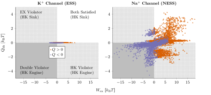
Figure 5: The two channel models compared via their nonequilibrium excess work and housekeeping heat distributions, respectively, in response to the spike protocol drive. Nonzero values of $Q_{\textnormal{hk}}$ indicate violations of the Crooks DFT Eq. (13), where the corrected NESS DFT Eq. (15) is needed. In addition, the axes here are of quantities with associated independent second laws; see Eqs. (20) and (23). And so, the labeled quadrants carry thermodynamic (and, in this case, biophysical) meaning as single-shot violations of each statistical second law.

Plotting housekeeping heat against excess work in Fig. 5 directly visualizes the independent kinds of negative entropy trajectories: where $\mathcal{W}_{\textnormal{ex}}<0$, we have single-shot violations of the familiar second law. In the isothermal environment of the ion channel models, trajectories for which this is the case imply channels that, under the spike protocol’s drive, funnel energy to the work reservoir. Where $\mathcal{Q}_{\textnormal{hk}}<0$, however, we have a new kind of second law violation unique to the NESS setting: in context, these are channels which have taken energy from the heat bath to maintain NESS conditions, rather than dissipated to it. For this reason, in Fig. 5, we label these quadrants “housekeeping (HK) engines.” Where total heat is also negative, the channel as a whole functions as a “total heat engine,” but—notably—these possibilities are independent of one and other. To take but one example: the negative total heat trajectories of the first quadrant act as heat engines, yet the housekeeping part of their total heat remains dissipative.

As Fig. 5 shows, the additional dimension of thermodynamic behavior afforded by nonzero housekeeping heat and its associated second law gives rise to a number of otherwise inaccessible combinations. Driving the channels according to the biologically-plausible spike protocol also reveals a greater range of possible Crooks DFT violations than did the more artificial pulse-driven result of Ref. riechersFluctuationsWhenDriving2017 , with only several violations. Taken together, Fig. 5 reveals a rich taxonomy of thermodynamic behaviors for the Na⁺ channel—behaviors that are not reflected (indeed, flattened) in the K⁺ channel or, indeed, in any ESS system, where Crooks’ DFT is satisfied and $\mathcal{Q}_{\textnormal{hk}}=0$. In particular, there are four functionally-distinct thermodynamic quadrants, corresponding to the positive and negative values of $\mathcal{Q}_{\textnormal{hk}}$ and $\mathcal{W}_{\textnormal{ex}}$, and labeled by their excess and housekeeping functionality on the K⁺ channel plot for clarity.

To be clear, each point on these plots corresponds to a single trajectory-reverse pair that itself is a valid trajectory class. Yet, (i) the samples themselves may be taken from a special class—for the Na⁺ channel we explicitly exclude resource-divergent trajectories—and (ii) any subsample on the plot corresponds to its own valid trajectory class as well.

The clustering of realized $Q_{\textnormal{hk}}$ in Fig. 5 reveals additional structure in Crooks DFT violations not previously observed. Apparently, there are distinct thermodynamic mechanisms that generate the violations. These result directly from the relative frequencies of transitions as functions of the driving protocol.

To lend additional insight into this structure, Fig. 6 plots the one-step rates of $Q_{\textnormal{hk}}$ production for each allowed transition in our modified Na⁺ channel. The A3 $\leftrightarrow$ A2 transition pair is the only one of this dynamic that is fully detailed-balanced for all inputs; the A2 $\leftrightarrow$ A1 pair is nearly detailed-balanced, with very small housekeeping heat production. By comparison, both of the remaining transitions strongly violate detailed balance, and so contribute the bulk of the nonzero $Q_{\textnormal{hk}}$.

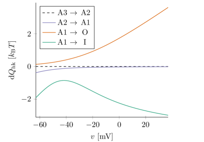
Figure 6: Na⁺ channel transition rates of housekeeping heat $Q_{\textnormal{hk}}$ as functions of transmembrane potential. The total housekeeping heat along any stochastic trajectory, driven by any protocol, is the sum of these values with the associated state transition-protocol parameter pairs here.

Physically, the latter two correspond to transitions directly to/from the open and inactivated channel states. Interestingly, their violations run in opposite directions. On the one hand, the A1 $\rightarrow$ O transition dissipates housekeeping heat to the thermal environment—indeed, more as the membrane voltage rises. On the other hand, the A1 $\rightarrow$ I transition describes the “ball and chain” that plugs the channel without opening, leaving no opportunity for Na⁺ current to flow. Thermodynamically, this transition actually absorbs housekeeping heat from the thermal environment. Since the housekeeping heat production rate is odd under transition reversal, these roles are reversed for the reverse transitions. Thus, the results shown in Fig. 5 arise directly from integrating those in Fig. 6 according to each trajectory-protocol pair.

As a final consideration, we note that the ESS TCFT (and so the Crooks DFT) do not claim to be valid for NESS systems. That said, our results visually verify the facts that the NESS generalization both extends the range of validity of the TCFT and reduces in the correct way for ESS systems.

That we have a trajectory class form for the NESS TCFT, captured in our Eq. (24), imports its ESS progenitor’s flexibility. That is, we need capture neither individual trajectory-level information to verify the DFT nor accurately sample the full trajectory space for an IFT.

That said, experimental verification remains a significant challenge. Generalizing to NESS systems requires not only the excess work distribution but housekeeping heats as well. Indeed, these results suggest that carefully considering how to measure housekeeping dissipation is crucial to characterizing fluctuations in NESS systems. As Fig. 5 demonstrates, improper accounting leads in general to TCFT violations and, if the ESS FTs are used to estimate free energy differences, to potentially drastically mischaracterizing the system of interest.

V.2 Average excess energetics

Despite the channels’ distinct thermodynamic functioning as revealed by the TCFT, we can compare the channels’ adaptive energetics via the excess works and heats. We begin by directly calculating the full trajectory averages, obtaining for discrete time:

$$-\expectationvalue{\mathcal{Q}_{\textnormal{ex}}} =\sum_{n=0}^{N-1}\innerproduct{\mu\pqty{t_{n+1}}-\mu\pqty{t_{n}}}{\phi_{\alpha_{n}}}\textnormal{ and}$$ (35)

$$\expectationvalue{\mathcal{W}_{\textnormal{ex}}} =\sum_{n=0}^{N-1}\innerproduct{\mu\pqty{t_{n}}}{\mu\pqty{t_{n}}}{\phi_{\alpha_{n+1}}-\phi_{\alpha_{n}}}\textnormal{,}$$ (36)

in agreement with Ref. riechersFluctuationsWhenDriving2017 . As above, we set the initial distributions to the local stationary distribution for convenience. Armed with the discrete protocols, time steps, and starting distributions, we directly evaluate the mixed states [Eq. (25)] and steady-state distributions [Eq. (26)] for each time step. These are all that is needed to calculate $\expectationvalue{\mathcal{Q}_{\textnormal{ex}}}$ and $\expectationvalue{\mathcal{W}_{\textnormal{ex}}}$ via Eqs. (35) and (36).

Figs. 7 and 8 give the simulation results for excess heat.

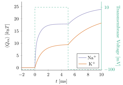
Figure 7: Excess heats (solid lines) for both channels under the pulse protocol (dashed line). The K⁺ channel is less dissipative. Both expend energy as they relax to environmentally-induced steady states.

First, driven by the pulse, the K⁺ channel dissipates less excess heat over the course of this protocol. Its rate of relaxation to steady state—corresponding to constant epochs in the protocol—appears slower than the Na⁺ channel’s on the jump from $-100$ to $10$ mV, but faster on the subsequent drop back down to $-100$ mV.

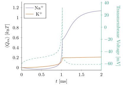
Figure 8: Excess heats (solid lines) for both channels driven by the spike protocol (dashed line). Under this more biologically realistic protocol, the Na⁺ dissipates significantly more than the K⁺ channel and does so responding much more rapidly to changes in membrane voltage. This suggests a tradeoff between the speed of the channel’s response and its dissipation, one not necessarily present in the more artificial pulse protocol.

The spike protocol paints a very different picture. Here, while the Na⁺ channel still dissipates (in this case, significantly) more over the course of the protocol, it also appears to respond much more quickly to changes in the protocol than does the K⁺ channel. A tradeoff appears: the cost of the Na⁺ channel adapting more quickly to its environment is that it dissipates more in the process. This did not arise when driven by the pulse protocol. (Likely, this is due to that protocol operating outside of the “normal” voltage range for these channels—by dropping as low as $-100$ mV.)

Besides showcasing a detailed energetic comparison between different channels, the discrepancy between the pulse- and spike-driven behaviors demonstrate that in vivo thermodynamic response can qualitatively differ from that elicited by voltage-clamp experiments.

The corresponding results for excess work are given in Figs. 9 and 10. Unlike excess heat, the excess work is not sensitive to the timescales of each channel’s relaxation to steady state. Instead, it tracks environmental entropy produced by the external drive. Yet it is still sensitive to the dynamics of the individual channel [per Eq. (8)], and this sensitivity is reflected in the thermodynamic responses.

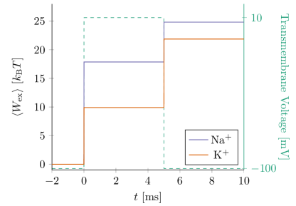
Figure 9: Excess works (solid lines) for both channels under the pulse protocol (dashed line). Unlike excess heat, excess work is only done upon change in the driving parameter. Thus, we see changes only at the pulse’s rise and fall. Much more excess work is done on the Na⁺ channel than on the K⁺ during the rise of the pulse, but these roles are reversed on its fall. Over the entire protocol, the Na⁺ channel produces (slightly) more excess environmental entropy.

As in the excess heat calculations, there is a difference in behavior between the pulse and spike protocols. In the former, the K⁺ channel and Na⁺ channels trade off under the rise and fall of the pulse. Driven by the spike protocol, however, the Na⁺ channel induces more environmental entropy production across the board, though they track extremely closely until the peak and reset phases of the action potential spike. This reflects not only the larger potential for dissipation in the Na⁺ channel under the spike protocol, but highlights where during the protocol most of the difference arises.

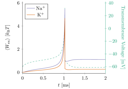
Figure 10: Excess works (solid lines) for both channels under the spike protocol (dashed line). We see that more excess work is done on the Na⁺ channel across the board. This corresponds to larger environmental entropy production and indicates a greater potential for dissipated work in the Na⁺ channel. However, we also see that up until the peak and reset phases of the action potential spike, they track very closely before diverging.

To reiterate, while excess heat is an energetic signature of relaxation to steady state, these calculations do not assume the system ever reaches such a steady state. While the pulse protocol allows each of the channels to do so, over the course of the spike we see a dynamic dissipation in the two channels—this is energy expended while attempting to reach an ever-evolving steady-state target. We close by highlighting that our theoretical developments enabled quantitatively comparing the channels’ adaptive energetics under realistic environmental stimuli—captured in our Fig. 8—despite the departures in their underlying steady-state dissipation.

VI Conclusion

We reviewed and extended the techniques of stochastic thermodynamics, culminating in a TCFT for NESSs, and even, for nonthermal stochastic processes. Using these, we analyzed the adaptive and homeostatic energetic signatures of two neurobiological systems—systems key to propagating action potentials in mammalian neurons. Along the way, we developed a toolkit for probing the nonequilbrium thermodynamics in a broad range of mesoscopic complex systems that requires little in the way of restrictive assumptions.

Our results exposed a new quantitative structure in how systems appear to violate equilibrium steady-state assumptions, both warning against and elucidating the consequences of inappropriately assuming detailed-balanced dynamics. In this, they suggest a need for both our corrected and generalized TCFT and new experimental tools.

Specifically, for nonequilibrium steady-state systems, tracking housekeeping entropy production is crucial to extracting functionally relevant thermodynamics and observing an additional kind of second law dynamics. While experimental tests have verified Eq. (20), they do not allow for observing the housekeeping thermodynamics, which play an important and independent part in assessing a system’s functionality.

Our simulations of the averaged excess energetics, in contrast, show how to compare specific aspects of a system’s functionality—the adaptive energetics—despite what are in this case infinite differences in the steady state behavior. In essence, these tools allow us to “cleave off” the divergence in the Na⁺ model’s housekeeping heat and still compare the channels’ adaptation to environmental drive on equal footing. Finally, the spike protocol simulations also identified what would not be observed in traditional patch-clamp experiments on ion channels, namely detailed differences in response to each segment of an action potential.

Taken together, our development and associated numerical experiments revealed a rich—and, indeed, necessary—set of tools with which to probe the nonequilibrium dynamics of mesoscopic complex systems.

Appendix A NESS TCFT Derivation

In addition to requiring a unique stationary distribution for each protocol value, we assume that for any $x_{0:N}\in\mathcal{X}^{N+1}$:

1. $x_{N:0}\in\mathcal{X}^{N+1}$,

2. $\mathcal{P}_{\bm{\mu}_{\textnormal{F}}}\pqty{x_{0:N}}\neq 0\implies\mathcal{P}_{\bm{\mu}_{\textnormal{F}}}\pqty{x_{N:0}}\neq 0$, and

3. $\mathcal{R}_{\bm{\mu}_{\textnormal{R}}}\pqty{x_{N:0}}\neq 0\implies\mathcal{R}_{\bm{\mu}_{\textnormal{R}}}\pqty{x_{0:N}}\neq 0$.

The second and third requirements, in particular, forbid one-way-only transitions in the discrete-time dynamic. Once we derive the TCFT, we will discuss the edge cases of completely irreversible trajectories.

Given the preceding constraints, a slightly rearranged form of Ref. riechersFluctuationsWhenDriving2017 ’s NESS DFT reads:

$$\mathcal{R}_{\bm{\mu}_{\textnormal{R}}}\pqty{x_{N:0}}=\mathcal{P}_{\bm{\mu}_{\textnormal{F}}}\pqty{x_{0:N}}\,\mathrm{e}^{-\pqty{\mathcal{W}_{\textnormal{ex}}+\mathcal{Q}_{\textnormal{hk}}-\Delta\mathcal{F}^{\textnormal{nss}}}}~{}.$$

We wish to integrate both sides over a trajectory class—the measurable subset $C\subseteq\mathcal{X}^{N+1}$ of trajectories. We also define the reverse trajectory class $C_{\textnormal{R}}\stackrel{{\scriptstyle.}}{{=}}\set{x_{N:0}\,}{\,x_{0:N}\in C}$. The following derivation mimics that of Ref. Wims19a after their Eq. (F3).

Integrating the lefthand side gives:

$$\int \bqty{x_{0:N}\in C}\,\mathcal{R}_{\bm{\mu}_{\textnormal{R}}}\pqty{x_{N:0}}\differential{x_{0:N}}$$

$$=\int\bqty{x_{0:N}\in C}\,\mathcal{R}_{\bm{\mu}_{\textnormal{R}}}\pqty{x_{N:0}}\differential{x_{N:0}}$$

$$=\int\bqty{x_{N:0}\in C_{\textnormal{R}}}\,\mathcal{R}_{\bm{\mu}_{\textnormal{R}}}\pqty{x_{N:0}}\differential{x_{N:0}}$$

$$=\mathcal{R}_{\bm{\mu}_{\textnormal{R}}}\pqty{C_{\textnormal{R}}}~{},$$

where $[\cdot]$ is the Iverson bracket.

Integrating the righthand side gives:

$$\int \bqty{x_{0:N}\in C}\,\mathcal{P}_{\bm{\mu}_{\textnormal{F}}}\pqty{x_{0:N}}\,\mathrm{e}^{-\pqty{\mathcal{W}_{\textnormal{ex}}+\mathcal{Q}_{\textnormal{hk}}-\Delta\mathcal{F}^{\textnormal{nss}}}}\differential{x_{0:N}}$$

$$=\int\mathcal{P}_{\bm{\mu}_{\textnormal{F}}}\pqty{x_{0:N}\cap C}\,\mathrm{e}^{-\pqty{\mathcal{W}_{\textnormal{ex}}+\mathcal{Q}_{\textnormal{hk}}-\Delta\mathcal{F}^{\textnormal{nss}}}}\differential{x_{0:N}}$$

$$=\mathcal{P}_{\bm{\mu}_{\textnormal{F}}}\pqty{C}\times$$

$$\qquad\int\mathcal{P}_{\bm{\mu}_{\textnormal{F}}}\left(x_{0:N}\,|\,C\right)\,\mathrm{e}^{-\pqty{\mathcal{W}_{\textnormal{ex}}+\mathcal{Q}_{\textnormal{hk}}-\Delta\mathcal{F}^{\textnormal{nss}}}}\differential{x_{0:N}}$$

$$=\mathcal{P}_{\bm{\mu}_{\textnormal{F}}}\pqty{C}\expectationvalue{\mathrm{e}^{-\pqty{\mathcal{W}_{\textnormal{ex}}+\mathcal{Q}_{\textnormal{hk}}-\Delta\mathcal{F}^{\textnormal{nss}}}}}_{C}~{},$$

where $\expectationvalue{\,\cdot\,}_{C}$ is the average over the trajectory class $C$. Thus, we have Eq. (24)—a TCFT for NESS systems, whose forward and reverse processes may start in arbitrary distributions:

$$\frac{\mathcal{R}_{\bm{\mu}_{\textnormal{R}}}\pqty{C_{\textnormal{R}}}}{\mathcal{P}_{\bm{\mu}_{\textnormal{F}}}\pqty{C}}=\expectationvalue{\mathrm{e}^{-\pqty{\mathcal{W}_{\textnormal{ex}}+\mathcal{Q}_{\textnormal{hk}}-\Delta\mathcal{F}^{\textnormal{nss}}}}}_{C}\textnormal{.}$$ (37)

Now, it remains to investigate the edge cases. Suppose that either (i) $\mathcal{P}_{\bm{\mu}_{\textnormal{F}}}\pqty{C}=0$ or (ii) $\mathcal{R}_{\bm{\mu}_{\textnormal{R}}}\pqty{C_{\textnormal{R}}}=0$, but not both. (The latter would amount to analyzing fluctuations for a pair of trajectories that never occur.) Since our probabilities are strictly nonnegative, the possible behaviors of the lefthand side are either $+\infty$ or $0$, respectively, by considering the limit of a vanishing probability. In case (i), by definition either $\mathrm{e}^{-\mathcal{Q}_{\textnormal{hk}}}\to+\infty$ or $\mathrm{e}^{\Delta\mathcal{F}^{\textnormal{nss}}}\to+\infty$ (or both) for each forward trajectory, yielding agreement with the lefthand side. In case (ii), similarly either $\mathrm{e}^{-\mathcal{Q}_{\textnormal{hk}}}\to 0$ or $\mathrm{e}^{\Delta\mathcal{F}^{\textnormal{nss}}}\to 0$ (or both) for each forward trajectory. Since the preceding derivation established the TCFT for all nondiverging cases, this establishes its validity even in the divergent limiting cases.

References

- (1) M. C. Cross and P. C. Hohenberg. Pattern formation outside of equilibrium. Rev. Mod. Phys., 65(3):851–1112, 1993.
- (2) E. H. Trepagnier, C. Jarzynski, F. Ritort, G. E. Crooks, C. J. Bustamante, and J. Liphardt. Experimental test of Hatano and Sasa’s nonequilibrium steady-state equality. Proc. Natl. Acad. Sci. U.S.A., 101(42):15038–15041, 2004.
- (3) M. Esposito. Stochastic thermodynamics under coarse graining. Phys. Rev. E, 85(4):041125, 2012.
- (4) C. Y. Gao and D. T. Limmer. Principles of low dissipation computing from a stochastic circuit model. arXiv:2102.13067, 2021.
- (5) Y. Oono and M. Paniconi. Steady State Thermodynamics. Prog. Theor. Phys. Suppl., 130:29–44, 1998.
- (6) With important exceptions, particularly in the first sense, under small perturbations from equilibrium Onsa31a ; Kond08a .
- (7) C. Jarzynski. Equilibrium free-energy differences from nonequilibrium measurements: A master-equation approach. Phys. Rev. E, 56(5):5018–5035, 1997.
- (8) C. Jarzynski. Nonequilibrium Equality for Free Energy Differences. Phys. Rev. Lett., 78(14):2690–2693, 1997.
- (9) G. E. Crooks. Entropy production fluctuation theorem and the nonequilibrium work relation for free energy differences. Phys. Rev. E, 60(3):2721–2726, 1999.
- (10) G. E. Crooks. Nonequilibrium Measurements of Free Energy Differences for Microscopically Reversible Markovian Systems. J. Stat. Phys., 90(5-6):1481–1487, 1998.
- (11) T. Hatano and S.-i. Sasa. Steady-State Thermodynamics of Langevin Systems. Phys. Rev. Lett., 86(16):3463–3466, 2001.
- (12) T. Speck and U. Seifert. Integral fluctuation theorem for the housekeeping heat. J. Phys. A: Math. Gen., 38(34):L581–L588, 2005.
- (13) P. M. Riechers and J. P. Crutchfield. Fluctuations When Driving Between Nonequilibrium Steady States. J. Stat. Phys., 168(4):873–918, 2017.
- (14) U. Seifert. Stochastic thermodynamics: From principles to the cost of precision. Physica A, 504:176–191, 2018.
- (15) P. Dayan and L. F. Abbott. Theoretical Neuroscience: Computational and Mathematical Modeling of Neural Systems. Computational Neuroscience. Massachusetts Institute of Technology Press, Cambridge, Mass, 2001.
- (16) J. Schnakenberg. Network theory of microscopic and macroscopic behavior of master equation systems. Rev. Mod. Phys., 48(4):571–585, 1976.
- (17) A. B. Boyd, D. Mandal, and J. P. Crutchfield. Identifying Functional Thermodynamics in Autonomous Maxwellian Ratchets. New J. Phys., 18(2):023049, 2016.
- (18) A. B. Boyd, D. Mandal, and J. P. Crutchfield. Thermodynamics of Modularity: Structural Costs Beyond the Landauer Bound. Phys. Rev. X, 8(3):031036, 2018.
- (19) A. M. Jurgens and J. P. Crutchfield. Functional thermodynamics of Maxwellian ratchets: Constructing and deconstructing patterns, randomizing and derandomizing behaviors. Phys. Rev. Research, 2(3):033334, 2020.
- (20) T. M. Cover and J. A. Thomas. Elements of Information Theory. Wiley-Interscience, second edition, 2006.
- (21) J. P. Sethna. Entropy, Order Parameters, and Complexity. Oxford Master Series in Physics. Oxford University Press, Oxford, second edition, 2021.
- (22) R. E. Spinney and I. J. Ford. Nonequilibrium Thermodynamics of Stochastic Systems with Odd and Even Variables. Phys. Rev. Lett., 108(17):170603, 2012.
- (23) J. Yeo, C. Kwon, H. K. Lee, and H. Park. Housekeeping entropy in continuous stochastic dynamics with odd-parity variables. J. Stat. Mech., 2016(9):093205, 2016.
- (24) R. J. Harris and G. M. Schütz. Fluctuation theorems for stochastic dynamics. J. Stat. Mech., 2007(07):P07020–P07020, 2007.
- (25) G. Wimsatt, O.-P. Saira, A. B. Boyd, M. H. Matheny, S. Han, M. L. Roukes, and J. P. Crutchfield. Harnessing fluctuations in thermodynamic computing via time-reversal symmetries. Phys. Rev. Res., 3(3):033115, 2021.
- (26) U. Çetiner, O. Raz, S. Sukharev, and C. Jarzynski. Recovery of Equilibrium Free Energy from Nonequilibrium Thermodynamics with Mechanosensitive Ion Channels in E. coli. Phys. Rev. Lett., 124(22):228101, 2020.
- (27) C. Jarzynski. Rare events and the convergence of exponentially averaged work values. Phys. Rev. E, 73(4):046105, 2006.
- (28) G. Hummer and A. Szabo. Free energy reconstruction from nonequilibrium single-molecule pulling experiments. Proc. Natl. Acad. Sci. U.S.A., 98(7):3658–3661, 2001.
- (29) J. Liphardt, S. Dumont, S. B. Smith, I. Tinoco, and C. Bustamante. Equilibrium Information from Nonequilibrium Measurements in an Experimental Test of Jarzynski’s Equality. Science, 296(5574):1832–1835, 2002.
- (30) C. Jarzynski. Work Fluctuation Theorems and Single-Molecule Biophysics. Prog. Theor. Phys. Suppl., 165:1–17, 2006.
- (31) U. Seifert. Stochastic thermodynamics, fluctuation theorems and molecular machines. Rep. Prog. Phys., 75(12):126001, 2012.
- (32) D. Collin, F. Ritort, C. Jarzynski, S. B. Smith, I. Tinoco, and C. Bustamante. Verification of the Crooks fluctuation theorem and recovery of RNA folding free energies. Nature, 437(7056):231–234, 2005.
- (33) S. Lahiri and A. M. Jayannavar. Fluctuation theorems for excess and housekeeping heat for underdamped Langevin systems. Eur. Phys. J. B, 87(9):195, 2014.
- (34) D. Mandal, K. Klymko, and M. R. DeWeese. Entropy Production and Fluctuation Theorems for Active Matter. Phys. Rev. Lett., 119(25):258001, 2017.
- (35) T. M. Cover and J. A. Thomas. Elements of Information Theory. Wiley-Interscience, New York, second edition, 2006.
- (36) P. M. Riechers and M. Gu. Initial-state dependence of thermodynamic dissipation for any quantum process. Phys. Rev. E, 103(4):042145, 2021.
- (37) C. A. Vandenberg and F. Bezanilla. A sodium channel gating model based on single channel, macroscopic ionic, and gating currents in the squid giant axon. Biophys. J., 60(6):1511–1533, 1991.
- (38) O.-P. Saira, M. H. Matheny, R. Katti, W. Fon, G. Wimsatt, J. P. Crutchfield, S. Han, and M. L. Roukes. Nonequilibrium thermodynamics of erasure with superconducting flux logic. Phys. Rev. Research, 2(1):013249, 2020.
- (39) A. L. Hodgkin and A. F. Huxley. A quantitative description of membrane current and its application to conduction and excitation in nerve. J. Physiol., 117(4):500–544, 1952.
- (40) K. Pal and G. Gangopadhyay. Dynamical characterization of inactivation path in voltage-gated Na${̂+}$ ion channel by non-equilibrium response spectroscopy. Channels, 10(6):478–497, 2016.
- (41) E. Marban, T. Yamagishi, and G. F. Tomaselli. Structure and function of voltage-gated sodium channels. J. Physiol., 508(3):647–657, 1998.
- (42) E. M. Izhikevich. Dynamical Systems in Neuroscience: The Geometry of Excitability and Bursting. Computational Neuroscience. The MIT Press, first edition, 2006.
- (43) E. M. Izhikevich. Simple model of spiking neurons. IEEE Trans. Neural Netw., 14(6):1569–1572, 2003.
- (44) L. Onsager. Reciprocal relations in irreversible processes, I". Phys. Rev., 37(4):405–426, 1931.
- (45) D. Kondepudi. Introduction to Modern Thermodynamics. Wiley, Chichester, 2008.