Joint Offloading Decision and Resource Allocation for Vehicular Fog-Edge Computing Networks: A Contract-Stackelberg Approach

Abstract

With the popularity of mobile devices and development of computationally intensive applications, researchers are focusing on offloading computation to Mobile Edge Computing (MEC) server due to its high computational efficiency and low communication delay. As the computing resources of an MEC server are limited, vehicles in the urban area who have abundant idle resources should be fully utilized. However, offloading computing tasks to vehicles faces many challenging issues. In this paper, we introduce a vehicular fog-edge computing paradigm and formulate it as a multi-stage Stackelberg game to deal with these issues. Specifically, vehicles are not obligated to share resources, let alone disclose their private information (e.g., stay time and the amount of resources). Therefore, in the first stage, we design a contract-based incentive mechanism to motivate vehicles to contribute their idle resources. Next, due to the complicated interactions among vehicles, road-side unit (RSU), MEC server and mobile device users, it is challenging to coordinate the resources of all parties and design a transaction mechanism to make all entities benefit. In the second and third stages, based on Stackelberg game, we develop pricing strategies that maximize the utilities of all parties. The analytical forms of optimal strategies for each stage are given. Simulation results demonstrate the effectiveness of our proposed incentive mechanism, reveal the trends of energy consumption and offloading decisions of users with various parameters, and present the performance comparison between our framework and existing MEC offloading paradigm in vehicular networks.

I Introduction

The development of Internet of Things and wireless communication technologies facilitates the emergence of computationally intensive applications with requirements of low latency and real-time processing, such as computer vision, natural language processing and autonomous driving. However, it is difficult for mobile devices with limited resources to provide required quality of service (QoS) for users [1].

Plenty of attempts have been made to offload computing tasks to the remote cloud server [2]. Although cloud computing can significantly improve computational performance, the long distance transmission may lead to considerable overhead and large latency [3]. By contrast, MEC with low cost servers in the vicinity of users, is a promising solution to computation offloading.

However, the computing resources of MEC server are usually constrained. Offloading computationally intensive tasks to these servers may cause low QoS, especially when the server is bursting with requests. Therefore, it is urgent to expand the resource capacity of MEC servers by exploiting idle resources from existing network entities and then effectively scheduling them for better services. Besides, energy-efficient optimization is also required for large-scale deployment and sustainable development of edge computing [4].

Recently, it is observed that vehicles with abundant idle computing resources can be organized into a vehicular fog computing (VFC) network so as to improve urban communication and computing capabilities [5]. In our daily life, many vehicles stay in the parking lot for a long time, or move slowly on the street. Due to their large number, long-term stay or slow movement, and relatively fixed location, vehicles in the urban area are ideal candidates for static backbone network and edge servers. In addition to the basic functions of computation offloading, such as providing users with computing, storage and application services, VFC also has the characteristics of low deployment cost, proximity to users, dense geographical distribution and so on. In this paper, we propose to utilize urban vehicles’ idle resources for computation offloading.

Nevertheless, there exist some challenging issues to be addressed. Firstly, vehicles are self-interested and have no obligation to share their idle resources. Therefore, a carefully designed incentive mechanism with reasonable rewards is indispensable. Additionally, vehicles are intuitively reluctant to disclose their private information, which creates an information asymmetry between vehicles and the organizer of VFC network like RSU. Secondly, the interactions among vehicles, RSU, the MEC server and mobile device users are complicated and difficult to model, due to their rationality and selfishness, and the tight coupling between resource demands and resource provisions. Thirdly, in order to realize a real-time and scalable computation offloading framework, an effective algorithm for joint offloading decision and resource allocation is preferred.

Motivated by the above issues, we introduce a new computing paradigm, named vehicular fog-edge computing (VFEC). In particular, a multi-stage Stackelberg game with an incentive mechanism is proposed to model the VFEC scenario. In a long-term market, RSU rents computing resources from vehicles. In this process, the information superiority over RSU for vehicles hinders the realization of Pareto optimal configuration. Based on contract theory, we design incentive mechanism to properly handle this problem. By designing a series of contract items for vehicles to choose from, the contract can reveal the respective types of vehicles, make up for the influence of information asymmetry, and maximize the utilities of two sides of trade. On the other hand, the transaction between RSU and the MEC server, as well as between the MEC server and users, can be considered as a short-term market, which involves various interactions such as publishing prices, offloading decision-making and computing resources purchase. Stackelberg game is suitable for modelling this short-term, complex and dynamic process. Moreover, the solution to equilibrium of Stackelberg game only needs one round of operations, instead of the iterative algorithms commonly used in some auctions and non-cooperative games. This is good news for the time-varying computation offloading service market.

The main contributions of this paper are listed below.

• We propose a vehicular fog-edge computing paradigm to utilize urban vehicles for computation offloading, and develop a multi-stage Stackelberg game with an incentive mechanism to model the interactions among RSU, MEC server and mobile device users.

• We design a contract-based incentive mechanism for RSU to manage the idle computing resources of nearby vehicles. In order to overcome the information asymmetry between vehicles and RSU, the contract items are designed carefully not only to maximize the utility of RSU, but also to satisfy individual rationality and incentive compatibility of vehicles.

• The analytical forms of optimal strategies for each stage of the transaction are given. Numerical evaluation is conducted, which demonstrates the effectiveness of our proposed algorithms, reveal the trends of energy consumption and offloading decisions of users with various parameters.

The rest of this paper is organized as follows. Related works are listed in Section II. Section III describes the system model. Section IV introduces the multi-stage Stackelberg game with a contract-based incentive mechanism. The optimal algorithms are presented elaborately in Section V. The simulation results are shown and interpreted in Section VI. Finally, we conclude this paper in Section VII.

II Related Works

MEC has recently attracted widespread attention from academia and industry. MEC servers are located on the edge of wireless network with more computing and storage resources than mobile terminals. Many existing works focus on MEC offloading in wireless networks, some of which are dedicated to minimize energy consumption [4, 6, 7, 8, 9], reduce latency [10, 11], or optimize a weighted objective of energy consumption and delay [12, 13]. In addition, most of the above works optimize resource allocation [8] or joint computation offloading and resource allocation [4, 6, 7, 8, 9, 12, 13] for MEC offloading in heterogeneous cellular networks. Due to the roll out of 5G mobile networks and Internet of Things, numerous and diverse users, servers and applications coexist in MEC systems. Therefore, server deployment and resource allocation become quite complicated in such system. Rodrigues et al. presented the utilization of Machine Learning (ML) to tackle these challenges in [14] and [15].

Thanks to MEC’s high computational efficiency and low communication delay, some works have deployed MEC server in vehicular networks, and aim to better support computationally intensive services with requirements of low latency and real-time processing [16]. In [17], Liu et al. provided an overview of Vehicular Edge Computing (VEC). A mobility-aware computation offloading design for MEC-based vehicular networks was studied in [18]. Due to the limited computing resources of single MEC server and high requirements for timely task processing of a large amount of computations in the emerging mobile applications, some works focus on MEC cooperation or grouping. For instance, a cloud-MEC collaborative computation offloading scheme in vehicular networks was presented in [19]. Considering the cooperative utilization of computing resources of MEC/cloud servers, Dai et al. solved a distributed task assignment problem [20]. Based on game theory, a noncooperative game-based strategy selection algorithm was presented in [21] to realize MEC grouping for task offloading, and a multi-user noncooperative computation offloading game was formulated in [22] to adjust the offloading probability of each vehicle. Besides, some works utilize neighbouring vehicles with idle computing resources to provide offloading opportunities to other vehicles having limited computing capabilities [23, 24, 25]. Among them, in [23], Gu et al. addressed the task offloading between MEC servers deployed at RSUs and vehicles with excessive computing resources. By treating vehicles as edge computing infrastructure, Qiao et al. introduced a vehicular edge multi-access network and constructed a cooperative and distributed computing architecture [24]. In [25], both an autonomous vehicular edge (AVE) which shares neighbouring vehicles’ available resources and a hybrid vehicular edge cloud (HVC) which shares accessible resources of RSUs and cloud were introduced. Hou et al. in [26] proposed an edge-computing-enabled software-defined Internet of vehicles (EC-SDIoV) architecture to efficiently orchestrate the heterogeneous edge computing nodes, and provide reliable and low-latency computation offloading, where partial offloading, reliable task allocation and the reprocessing mechanism are jointly considered. In order to deal with the dynamic vehicular environment, Shi et al. in [27] proposed a priority-aware task offloading scheme in the context of vehicular fog computing, where a soft actor-critic method is developed to select the service vehicles and publish dynamic prices. The algorithm in [27] achieved more robust and sample-efficient performance in task completion ratio and offloading delay. More and deeper issues of MEC are surveyed in [28] toward future vehicular networks.

Recently, parked and slow moving vehicles have attracted much attention to improve the performance of vehicular networks. Malandrino et al. investigated the possibility of exploiting parked vehicles to extend the RSU service coverage [29]. In [30], a game theoretic framework of content delivery which utilized parked vehicles was proposed. Sun et al. considered the parked vehicles as relay nodes in [31]. Observing that parked or slow moving vehicles have rich and under-utilized resources for task execution, some works studied utilizing vehicles to develop new computing paradigms [5, 32]. Aiming to minimize the average response time for events reported by vehicles, Wang et al. put forward a feasible solution which enables offloading by moving and parked vehicles for real-time traffic management [33]. With adopting parked vehicles for computation offloading, an energy-efficient parked vehicular computing (PVC) paradigm was developed in [34].

Different from existing works, this paper focuses on some challenging issues. First, vehicles have no obligation and willingness to share their idle computing resources. Second, there is information asymmetry between vehicles and the organizer of VFC network, which makes it difficult to distinguish the qualification of vehicles. Therefore, it is necessary to design an incentive mechanism to reveal the types of vehicles, and encourage them to participate in the computation offloading with a certain reward. Third, the offloading service involves multiple transaction processes with multiple participants. How to coordinate the resources of all parties in an integrated way so that all entities can benefit is also a major challenge. In this paper, we introduce a vehicular fog-edge computing paradigm and formulate it as a multi-stage Stackelberg game to deal with these issues.

TABLE I: Key Notations and Definitions

Notation	Definition	Notation	Definition
$c_{i}$	the computation needed by user $i$’s task	$f_{i}^{thresh}$	a threshold of resources for judging whether user $i$ choose to offload its task or not
$d_{i}$	the size of input data of user $i$’s task	$f_{e}$	the computing resources of MEC server used for task offloading
$t_{i}^{\mathrm{max}}$	the maximum tolerable latency of user $i$’s task	$f_{RSU}$	the computing resources that the MEC server purchases from RSU
$f_{i}^{l}$	the local computing resources of user $i$	$e,e_{v}$	the unit monetary cost of server’s / vehicle’s energy consumption
$f_{e}^{\mathrm{max}}$	the computing resources of MEC server	$k$	the effective switched capacitance, which depends on the chip architecture
$f_{v}^{\mathrm{max}}$	the idle computing resources of each vehicle	$\theta_{m},m\in\{1,2,\ldots,M\}$	the type of a vehicle
$U_{i},U_{MEC},U_{RSU},U_{V_{m}}$	the utility of user $i$ / the MEC server / RSU / a type-$m$ vehicle	$l_{m}$	the number of type-$m$ vehicles near RSU
$p$	the price of MEC server’s computing resources	$f_{m}$	the computing resources that RSU rents from a type-$m$ vehicle
$c$	the price of computing resources collected by RSU	$p_{m}$	the rent for leased resources of a type-$m$ vehicle per unit of time
$f_{i}$	the quantity of resources that user $i$ purchases from the MEC server

III System Model

III-A Overview

We consider a small district in the urban area, where an MEC server, an RSU, some vehicles and some mobile device users are located. We assume that the connections between all involved entities are single hop.

There are $N$ mobile device users in this region, such as smart phones, vehicles, wearable devices and so on. We denote the ID set of these users as $\mathscr{N}=\{1,2,\ldots,N\}$. At some point, each user has a computationally intensive task to be completed, which is characterized by a tuple $(c_{i},d_{i},t_{i}^{\mathrm{max}}),\ \forall i\in\mathscr{N}$. $c_{i}$ represents the computation (in CPU cycles) needed by user $i$’s task. $d_{i}$ is the size of input data of user $i$’s task. $t_{i}^{\mathrm{max}}$ is the maximum tolerable latency of user $i$. $f_{i}^{l}$ denotes the local computing resources of user $i$ (in CPU cycles/s).

There exists an MEC server, whose computing resources, denoted as $f_{e}^{\mathrm{max}}$, are limited. A user may offload its task to the MEC server or execute it locally, depending on the price of resources and how fast its task will be completed.

The resources of MEC server are not always able to meet the needs of all users, which means high latency, expensive prices and low QoS. We may consider making full use of vehicular idle resources to improve users’ experience, where the resources are collected and scheduled by RSU.

All vehicles in this region, whether parking or moving slowly, can establish stable wireless connection with RSU via vehicle-to-infrastructure (V2I) communications. Each vehicle is equipped with an on-board-unit (OBU), which is not a simple device tracking the vehicle location and measuring its speed, but a mobile device with storage, communication and computing capabilities [35]. We assume that the total amount of idle resources owned by each vehicle, $f_{v}^{\mathrm{max}}$, is the same. After signing the contract, OBUs within the communication range of RSU can be organized into a fog cluster so as to enhance service capabilities.

In order to perform computation offloading efficiently after the MEC server has prepared computing resources and users have made their offloading decisions, the HVC architecture in [25] may be used, which designs a workflow that includes steps such as job caching, job scheduling, data transmission, job execution and result data transmission. Additionally, to facilitate the entire transaction process and take care of the interests in all parties to a fair and impartial manner, a third-party central controller is set up in the system, which is subordinate to a computation offloading operator. Its responsibilities include collecting global information, running the proposed algorithms, scheduling users’ tasks and transmitting control messages, etc. As mentioned earlier, this paper focuses on resource scheduling and users’ offloading decisions. The details of these implementations are beyond the scope of this paper and will be the direction of future work.

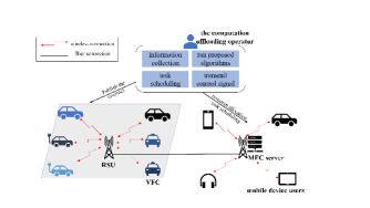
Figure 1: The vehicular fog-edge computing network architecture

III-B Three-stage Stackelberg game

In order to ensure that vehicles, RSU, the MEC server and users are willing to participate in computation offloading, we design a multi-stage Stackelberg game for this vehicular fog-edge computing paradigm. In this game, a contract-based incentive mechanism is developed for RSU to recruit the idle computing resources of vehicles, while the interactions between RSU and the MEC server, the MEC server and users are modeled as a multi-stage Stackelberg game.

Specifically, in the first stage, a contract-based trading mechanism is designed to employ vehicles for users’ task execution. The RSU acts as an employer who offers different contract items to vehicles, while each vehicle is an employee who selects a certain type of contract which suits it best. At the same time, RSU also acts as the leader of RSU-MEC Stackelberg game and announces the price of computing resources to the MEC server.

In the second stage, the MEC server is both the follower of RSU-MEC Stackelberg game and the leader of MEC-user Stackelberg game, determining the quantity of computing resources purchased from RSU and broadcasting the price of resources to all mobile device users.

In the third stage, all users are the followers of MEC-user Stackelberg game. Each user decides whether to offload its task and the quantity of computing resources purchased from the MEC server.

Note that since parked or slow moving vehicles are considered, the leasing of idle vehicular computing resources is a long-term market. In contrast, the deadline for a user’s task is shorter, so the RSU-MEC Stackelberg game and the MEC-user Stackelberg game are played slot by slot.

III-C Utility functions

mobile device users

The utility function of user $i$ is defined as

$$U_{i}(f_{i})=\frac{C}{t_{i}^{\mathrm{max}}}\ln\left(\frac{f_{i}}{f^{l}_{i}}+\delta\right)-pf_{i}.$$ (1)

In fact, users tend to purchase more computing resources to minimize delay. However, with the continuous growth of obtained resources, the shortened completion time is reduced, and the benefits of unit computing resource are gradually declining as well. That is, diminishing marginal effect appears. Therefore, the benefits of a user can be characterized by a concave function of the purchased computing resources over its local resources. So we may adopt a logarithmic function. $C>0$ is a constant, and $\tau_{i}\triangleq C/t_{i}^{\mathrm{max}}$ represents user $i$’s sensitivity to latency. $\delta\geq 1$, is to make sure that the logarithmic function has a positive value. $p$ denotes the price of MEC server’s computing resources, and $f_{i}$ is the quantity of resources that user $i$ purchases from the MEC server. The utility of a mobile device user is defined as the benefits of offloading service minus the expenditure of resources.

If user $i$ decides to execute its task locally, the completion time is

$$t_{i}^{l}=\frac{c_{i}}{f_{i}^{l}}.$$ (2)

Otherwise, user $i$ offloads its task to the MEC server. The completion time is composed of upload latency and execution delay. Then the completion latency for offloading user $i$’s task to the MEC server is

$$t_{i}^{e}=\frac{d_{i}}{r_{i}}+\frac{c_{i}}{f_{i}},$$ (3)

where $r_{i}$ represents the upload transmission rate from user $i$ to the MEC server. When $t_{i}^{e}<t_{i}^{l}$, user $i$ may prefer to offload its computationally intensive task to the MEC server. Let $f_{i}^{thresh}=\frac{c_{i}}{\frac{c_{i}}{f_{i}^{l}}-\frac{d_{i}}{r_{i}}}$. If

$$f_{i}>f_{i}^{thresh},$$ (4)

then user $i$ will choose to offload its task.

the MEC server

The utility function of the MEC server is defined as

$$U_{MEC}(p,f_{e},f_{RSU})=\sum_{i=1}^{N}pf_{i}-ekf_{e}^{2}-cf_{RSU},$$ (5)

where $f_{e}$ is the computing resources of MEC server used for task offloading, and $e$ denotes the unit cost of server’s energy consumption. $kf_{e}^{2}$ represents the energy of MEC server consumed by computation. Here, the energy consumption model of computation is referenced from [10]. $k$ is the effective switched capacitance, which depends on the chip architecture. In order to simplify expressions, let $k_{e}=ek$. $c$ denotes the price of resources collected by RSU, and $f_{RSU}$ is the computing resources that the MEC server purchases from RSU. The utility of MEC server is the revenues from users minus the energy cost and the expenditure of purchasing computing resources from the RSU.

the RSU

Before the contract is signed, we assume that RSU has obtained the current stay time of each vehicle within its communication range, which is denoted as $\theta_{v}^{\prime}$. The type of a vehicle $v$ is defined as the length of time it continues to park or stay, $\theta_{v}$. Of course, RSU prefers the vehicle who has a longer stay. Due to the existence of information asymmetry between vehicles and RSU, the latter does not know the exact types of former. However, through statistics on the historical data, RSU can obtain the probability cumulative function of vehicle stay time $F(t)$ about the timing in a day, vehicle position and other factors. Then we have:

$$P(\theta\geq\theta_{v}+\theta_{v}^{\prime}|\theta\geq\theta_{v}^{\prime})=\frac{1-F(\theta_{v}+\theta_{v}^{\prime})}{1-F(\theta_{v}^{\prime})}.$$ (6)

In order to facilitate the subsequent analysis, we discretize the type of vehicles into $M$ items: $\theta_{1},\theta_{2},\ldots,\theta_{M}$ with $\theta_{1}\leq\theta_{2}\leq\ldots\leq\theta_{M}$. Then it can be seen that RSU can calculate the probability distribution of the vehicles’ continued stay time at the current moment, $f(\theta_{m})$ with $\sum_{m=1}^{M}f(\theta_{m})=1$. Therefore, the number of type-$m$ vehicles near the RSU is $l_{m}=f(\theta_{m})L$, where $L$ is the total number of vehicles.

The utility function of RSU is

$$U_{RSU}(f_{m},p_{m},c)=cf_{RSU}-\sum_{m=1}^{M}l_{m}\theta_{m}p_{m},$$ (7)

where $p_{m}$ represents the rent for leased resources of a type-$m$ vehicle per unit of time. The utility of RSU is defined as payment from the MEC server minus the cost of renting computing resources from vehicles.

vehicles

The utility function of a type-$m$ vehicle is defined as

$$U_{V_{m}}(f_{m},p_{m})=\theta_{m}p_{m}-e_{v}kf_{m}^{2},$$ (8)

where $f_{m}$ denotes the quantity of computing resources offered by a type-$m$ vehicle, and $e_{v}$ is the unit monetary cost of vehicle’s energy consumption. The utility of a vehicle is the rewards from RSU minus the cost of energy consumption on computing.

IV Problem Formulation

IV-A Stage I

To motivate the vehicles to participate the transaction and select the contract item which fits their types best, the following IR and IC conditions should be satisfied [36].

Definition 1

[Individual Rationality (IR)] Since the vehicles are rational, IR condition committed a nonnegative utility to a vehicle if it accepts the contract item designed for its type. The IR conditions can be formulated as

$$\theta_{m}p_{m}-k_{v}f_{m}^{2}\geq 0,\ \forall m\in\{1,2,\cdots,M\}.$$ (9)

Similar to the MEC server, let $k_{v}=e_{v}k$ to simplify the derivation process.

Definition 2

[Incentive Compatibility (IC)] IC conditions guarantee that a type-$m$ vehicle will select the contract $(f_{m},p_{m})$, rather than any other contract items $(f_{j},p_{j}),\ \forall j\in\{1,2,\cdots,M\}\backslash\{m\}$. The IC conditions can be written as

$$\theta_{m}p_{m}-k_{v}f_{m}^{2}\geq\theta_{m}p_{j}-k_{v}f_{j}^{2},\\ \forall m,j\in\{1,2,\cdots,M\},m\neq j.$$ (10)

Meanwhile, the RSU also plays the leader of RSU-MEC Stackelberg game and announces the price of computing resources $c$ to the MEC server. We formulate the utility maximization problem of RSU as

$$\max_{f_{m},p_{m},c} U_{RSU}(f_{m},p_{m},c)$$ (11)

$$\mathrm{s.t.}\ \mathbf{C1:} c\geq 0$$

$$\mathbf{C2:} 0\leq f_{m}\leq f_{v}^{\mathrm{max}},\ \forall m\in\{1,2,\cdots,M\}$$

$$\mathbf{C3:} \sum_{m=1}^{M}l_{m}f_{m}\geq f_{RSU}$$

$$\mathbf{C4:} \eqref{eq:IR}$$

$$\mathbf{C5:} \eqref{eq:IC}$$

C3 ensures that the MEC server does not purchase more resources than the resources RSU renting from vehicles.

IV-B Stage II

In this transaction, the MEC server plays two roles. It is the follower of RSU-MEC Stackelberg game as well as the leader of MEC-user Stackelberg game. The MEC server determines computing resources $f_{RSU}$ purchased from the RSU and computing resources $f_{e}$ used locally based on the price of unit resources $c$ of RSU. At the same time, it broadcasts the price of unit resources $p$ to all mobile device users. We can describe the utility maximization problem of MEC server as

$$\max_{p,f_{e},f_{RSU}} U_{MEC}(p,f_{e},f_{RSU})$$ (12)

$$\mathrm{s.t.}\ \mathbf{C6:} p\geq 0$$

$$\mathbf{C7:} 0\leq f_{e}\leq f_{e}^{\mathrm{max}}$$

$$\mathbf{C8:} f_{RSU}\geq 0$$

$$\mathbf{C9:} f_{e}+f_{RSU}=\sum_{i=1}^{N}f_{i}$$

IV-C Stage III

The mobile device user $i$, as a follower of MEC-user Stackelberg game, determines the quantity of computing resources $f_{i}$ purchased from the MEC server based on the price $p$ to maximize its own utility. We can formulate the optimization problem of user $i$ as

$$\max_{f_{i}} U_{i}(f_{i})$$ (13)

$$\mathrm{s.t.}\ \mathbf{C10:} \eqref{eq:f_thresh}$$

V Optimal Algorithm

In this section, we use the backward induction method to analyze this multi-stage Stackelberg game and the contract-based incentive mechanism.

V-A Solution of Stage III

Since the utility function of user $i$ is a concave function, the zero point of its first derivative is the optimal solution. That is,

$$f_{i}^{\star}=\begin{cases}\frac{\tau_{i}}{p}-f_{i}^{l}\delta,\quad&p<\frac{\tau_{i}}{f_{i}^{l}\delta+f_{i}^{thresh}}\\ 0,\ &p\geq\frac{\tau_{i}}{f_{i}^{l}\delta+f_{i}^{thresh}}\end{cases}$$ (14)

We can see that if the price of computing resources is too high, i.e., $p\geq\frac{\tau_{i}}{f_{i}^{l}\delta+f_{i}^{thresh}}$, user $i$ is unwilling to offload its task.

V-B Solution of Stage II

Given the quantity of computing resources (14) purchased by users, we can substitute it into the utility function of MEC server. Note that $f_{i}^{\star}$ is a piecewise function, we introduce the following indicator variable for user $i$

$$\chi_{i}=\begin{cases}1,\quad&p<\frac{\tau_{i}}{f_{i}^{l}\delta+f_{i}^{thresh}}\\ 0,\quad&p\geq\frac{\tau_{i}}{f_{i}^{l}\delta+f_{i}^{thresh}}\end{cases}$$ (15)

Then (12) can be rewritten as

$$\max_{p,f_{e},f_{RSU},\chi} \sum_{i=1}^{N}\chi_{i}\left(\tau_{i}-f_{i}^{l}\delta p\right)-k_{e}f_{e}^{2}-cf_{RSU}$$ (16)

$$\mathrm{s.t.}\ \mathbf{C6} \mathbf{-C9}$$

$$\mathbf{C11} \mathbf{:}\ \chi_{i}\in\{0,1\},\ \forall i\in\mathscr{N}$$

where $\chi=[\chi_{1},\chi_{2},\cdots,\chi_{N}]^{\intercal}$. Since $\chi$ is a binary vector, and $p,f_{e},f_{RSU}$ are continuous variables, the optimization problem (16) is a mixed integer nonlinear programming problem. Given the indicator vector $\chi$, it is easy to verify that this problem is concave.

We assume that the users are sorted in the following order:

$$\frac{\tau_{1}}{f_{1}^{l}\delta+f_{1}^{thresh}} \geq\frac{\tau_{2}}{f_{2}^{l}\delta+f_{2}^{thresh}}$$ (17)

$$\geq\cdots$$

$$\geq\frac{\tau_{N}}{f_{N}^{l}\delta+f_{N}^{thresh}}.$$

According to (15), we can see that whether a user chooses to offload its task depends on the price of unit computing resources of MEC server, i.e., $p$. Further, in our transaction framework, $p$ depends on the price of unit computing resources of RSU, i.e., $c$. Thus, we consider a special case of (16), in which we assume that $c$ is small enough such that all users choose to participate in the offloading. That is, the indicators for all users are equal to $1$. Under this assumption, (16) can be rewritten as

$$\max_{p,f_{e},f_{RSU}} \sum_{i=1}^{N}\left(\tau_{i}-f_{i}^{l}\delta p\right)-k_{e}f_{e}^{2}-cf_{RSU}$$ (18)

$$\mathrm{s.t.}\ \mathbf{C6} \mathbf{-C8}\$$

$$\mathbf{\overline{C9}} \mathbf{:}\ \sum_{i=1}^{N}\left(\frac{\tau_{i}}{p}-f_{i}^{l}\delta\right)=f_{e}+f_{RSU}$$

Proposition 1

The optimal solution of (18) is

$$p^{\star}=\sqrt{\frac{c\sum_{i=1}^{N}\tau_{i}}{\delta\sum_{i=1}^{N}f_{i}^{l}}},$$ (19)

$$f_{e}^{\star}=\min\left\{\frac{c}{2k_{e}},f_{e}^{\mathrm{max}}\right\},$$ (20)

when $2k_{e}f_{e}^{\mathrm{max}}\leq T_{N}$, $f_{RSU}^{\star}$ is shown as

$$f_{RSU}^{\star}=\begin{cases}\left[\sqrt{\frac{\tau\Delta}{c}}-\Delta-\frac{c}{2k_{e}}\right]^{+},\ &c\leq 2k_{e}f_{e}^{\mathrm{max}}\\ \left[\sqrt{\frac{\tau\Delta}{c}}-\Delta-f_{e}^{\mathrm{max}}\right]^{+},\ &2k_{e}f_{e}^{\mathrm{max}}<c<T_{N}\end{cases}$$ (21)

when $2k_{e}f_{e}^{\mathrm{max}}>T_{N}$,

$$f_{RSU}^{\star}=\left[\sqrt{\frac{\tau\Delta}{c}}-\Delta-\frac{c}{2k_{e}}\right]^{+},\ 0\leq c<T_{N},$$ (22)

where $\tau=\sum_{i=1}^{N}\tau_{i},\Delta=\sum_{i=1}^{N}f_{i}^{l}\delta,T_{N}=\frac{\tau_{N}\sqrt{\delta\sum_{i=1}^{N}f_{i}^{l}}}{\left(f_{N}^{l}\delta+f_{N}^{thresh}\right)\left(\sum_{i=1}^{N}\tau_{i}\right)}$. The proof of this proposition is shown in part A of Appendix.

Proposition 2

The price of MEC server’s computing resources given by (19) and the quantity of computing resources purchased by the MEC server from RSU given by (21) and (22) are optimal solution of (16) if and only if $c<T_{N}$. The proof of Proposition 2 is shown in part B of Appendix.

Then the optimal solution of (16) is given by the following theorem.

Theorem 1

The optimal solution of (16) is

$$p^{\star}=\begin{cases}q_{N},\quad&c<T_{N}\\ q_{N-1},\quad&T_{N}\leq c<T_{N-1}\\ \quad\vdots\quad&\quad\vdots\\ q_{1},\quad&T_{2}\leq c<T_{1}\end{cases}$$ (23)

(i): $2k_{e}f_{e}^{\mathrm{max}}\geq T_{1}$,

$$f_{RSU}^{\star}=\begin{cases}\left[L_{N}-\frac{c}{2k_{e}}\right]^{+},\quad&c<T_{N}\\ \left[L_{N-1}-\frac{c}{2k_{e}}\right]^{+},\quad&T_{N}\leq c<T_{N-1}\\ \quad\vdots\quad&\quad\vdots\\ \left[L_{1}-\frac{c}{2k_{e}}\right]^{+},\quad&T_{2}\leq c<T_{1}\end{cases}$$ (24)

(ii): $2k_{e}f_{e}^{\mathrm{max}}\leq T_{N}$

$$f_{RSU}^{\star}=\begin{cases}\left[L_{N}-\frac{c}{2k_{e}}\right]^{+},\quad&c\leq 2k_{e}f_{e}^{\mathrm{max}}\\ \left[L_{N}-f_{e}^{\mathrm{max}}\right]^{+},\quad&2k_{e}f_{e}^{\mathrm{max}}<c<T_{N}\\ \left[L_{N-1}-f_{e}^{\mathrm{max}}\right]^{+},\quad&T_{N}\leq c<T_{N-1}\\ \quad\vdots\quad&\quad\vdots\\ \left[L_{1}-f_{e}^{\mathrm{max}}\right]^{+},\quad&T_{2}\leq c<T_{1}\end{cases}$$ (25)

(iii): $T_{N}<2k_{e}f_{e}^{\mathrm{max}}<T_{1}$ and $T_{o}\leq 2k_{e}f_{e}^{\mathrm{max}}<T_{o-1},\forall o\in\{2,3,\cdots,N\}$

$$f_{RSU}^{\star}=\begin{cases}\left[L_{N}-\frac{c}{2k_{e}}\right]^{+},\quad&c<T_{N}\\ \quad\vdots\quad&\quad\vdots\\ \left[L_{o}-\frac{c}{2k_{e}}\right]^{+},\quad&T_{o}\leq c\leq 2k_{e}f_{e}^{\mathrm{max}}\\ \left[L_{o}-f_{e}^{\mathrm{max}}\right]^{+},\quad&2k_{e}f_{e}^{\mathrm{max}}<c<T_{o-1}\\ \quad\vdots\quad&\quad\vdots\\ \left[L_{1}-f_{e}^{\mathrm{max}}\right]^{+},\quad&T_{2}\leq c<T_{1}\end{cases}$$ (26)

where $q_{k}=\sqrt{\frac{c\sum_{i=1}^{k}\tau_{i}}{\delta\sum_{i=1}^{k}f_{i}^{l}}},T_{k}=\frac{\tau_{k}\sqrt{\delta\sum_{i=1}^{k}f_{i}^{l}}}{\left(f_{k}^{l}\delta+f_{k}^{thresh}\right)\left(\sum_{i=1}^{k}\tau_{i}\right)},L_{k}=\sqrt{\frac{\left(\sum_{i=1}^{k}\tau_{i}\right)\left(\delta\sum_{i=1}^{k}f_{i}^{l}\right)}{c}}-\delta\sum_{i=1}^{k}f_{i}^{l},\ \forall k\in\{1,2,\cdots,N\}$.

Proof:

If $c<T_{N}$, the optimal solution of (16) is obtained by Proposition 2. For $c$ in other intervals, the solution can be obtained similarly as Proposition 2, and is thus omitted. ∎

The algorithm for optimal solution of Stage II is shown as below:

Algorithm 1 the optimal solution of Stage II

  Step 1: Initialize $k=N$;

  Step 2: Sort all users according to (17);

  Step 3: Compute $T_{k}=\frac{\tau_{k}\sqrt{\delta\sum_{i=1}^{k}f_{i}^{l}}}{\left(f_{k}^{l}\delta+f_{k}^{thresh}\right)\left(\sum_{i=1}^{k}\tau_{i}\right)}$;

  Step 4: Compare $T_{k}$ with $c$. If $c\geq T_{k}$, remove user $k$ from the game, set $k=k-1$, and go to step 3; otherwise, go to step 5;

  Step 5: According to Theorem 1, find the optimal solution $p^{\star}$ and $f_{RSU}^{\star}$.

V-C Solution of Stage I

It can be seen that the expression of $f_{RSU}^{\star}$ can be divided into three cases depending on the relationship between the values of $2k_{e}f_{e}^{\mathrm{max}}$ and $T_{k},\forall k\in\{1,2,\cdots,N\}$. Here, we only give the solving process of Stage I in the case of $2k_{e}f_{e}^{\mathrm{max}}\geq T_{1}$. The other two cases can be solved in similar ways. To solve the utility maximization problem of RSU (11), we substitute (24) into (11). Since the expression of $f_{RSU}^{\star}$ is piecewise, the problem is decomposed into $N$ subproblems. Assuming that $T_{k}\leq c<T_{k-1}$, (11) can be rewritten as:

$$\min_{f_{m},p_{m},c} \sum_{m=1}^{M}l_{m}\theta_{m}p_{m}-c\left(L_{k}-\frac{c}{2k_{e}}\right)$$ (27)

$$\mathrm{s.t.}\ \mathbf{C2,} \mathbf{C4,C5}$$

$$\mathbf{\overline{C1}:} T_{k}\leq c<T_{k-1}$$

$$\mathbf{\overline{C3}:} L_{k}-\frac{c}{2k_{e}}\leq\sum_{m=1}^{M}l_{m}f_{m}$$

$$\mathbf{C11:} L_{k}-\frac{c}{2k_{e}}\geq 0$$

The optimization problem (27) is difficult to solve due to $M$ IR constraints and $M(M-1)$ IC constraints. Below we propose several lemmas to simplify these constraints.

Lemma 1

For any feasible contract, if $\theta_{i}>\theta_{j}$, then we have $p_{i}>p_{j},\forall i,j\in\{1,2,\cdots,M\}$.

Lemma 2

For any feasible contract, $p_{i}>p_{j}$ if and only if $f_{i}>f_{j},\forall i,j\in\{1,2,\cdots,M\}$.

The above two lemmas have been proved in [36]. Then, we can reduce IR and IC constraints by the following lemmas.

Lemma 3

If the IR constraint of type-$1$ vehicles is satisfied, then all other IR constraints of type-$m$, $m\in\{2,3,\cdots,M\}$ vehicles are also satisfied. That is,

$$\theta_{m}p_{m}-k_{v}f_{m}^{2}\geq\theta_{1}p_{1}-k_{v}f_{1}^{2}\geq 0.$$ (28)

Lemma 4

The IC conditions can be reduced to the local downward incentive compatibility (LDIC) conditions and the local upward incentive compatibility (LUIC):

$$\theta_{m}p_{m}-k_{v}f_{m}^{2}\geq\theta_{m}p_{m-1}-k_{v}f_{m-1}^{2},\ \forall m\in\{2,3,\cdots,M\},$$ (29)

$$\theta_{m}p_{m}-k_{v}f_{m}^{2}\geq\theta_{m}p_{m+1}-k_{v}f_{m+1}^{2},\ \forall m\in\{1,2,\cdots,M-1\}.$$ (30)

Lemma 5

Under the optimal contract, all the LDIC constraints are active, and the IR constraint of type-$1$ vehicles is active as well. That is,

$$\theta_{m}p_{m}-k_{v}f_{m}^{2}=\theta_{m}p_{m-1}-k_{v}f_{m-1}^{2},\ \forall m\in\{2,3,\cdots,M\},$$ (31)

$$\theta_{1}p_{1}-k_{v}f_{1}^{2}=0.$$ (32)

Lemma 6

If all the LDIC constraints are active, then all the LUIC constraints are satisfied.

See the Appendix for proofs of above four lemmas.

Then, the IR and IC conditions are reduced to active type-$1$ IR constraint and active LDIC constraints. Note that $\mathbf{C11}$ is not concave, we transform $\mathbf{C11}$ to a concave function of $c$ $\mathbf{\overline{C11}}$. Thus, (27) can be rewritten as

$$\min_{f_{m},p_{m},c} \sum_{m=1}^{M}l_{m}\theta_{m}p_{m}-c\left(L_{k}-\frac{c}{2k_{e}}\right)$$ (33)

$$\mathrm{s.t.}\ \mathbf{\overline{C1},} \mathbf{C2,\overline{C3}}$$

$$\mathbf{\overline{C4}:} \theta_{1}p_{1}-k_{v}f_{1}^{2}=0$$

$$\mathbf{\overline{C5}:} \theta_{m}p_{m}-k_{v}f_{m}^{2}=\theta_{m}p_{m-1}-k_{v}f_{m-1}^{2},\ m\geq 2$$

$$\mathbf{\overline{C11}:} c\left(L_{k}-\frac{c}{2k_{e}}\right)\geq 0$$

$$\mathbf{C12:} 0\leq p_{1}\leq p_{2}\leq\cdots\leq p_{M}$$

Obviously, the optimization problem (33) is convex and can be solved by Lagrangian multiplier method. The Lagrangian function is defined as

$$\mathscr{L}= \sum_{m=1}^{M}l_{m}\theta_{m}p_{m}-c\left(L_{k}-\frac{c}{2k_{e}}\right)$$ (34)

$$+ \gamma(\theta_{1}p_{1}-k_{v}f_{1}^{2})+\beta\left(-cL_{k}+\frac{c^{2}}{2k_{e}}\right)$$

$$+ \sum_{m=2}^{M}\mu_{m}\left(\theta_{m}(p_{m-1}-p_{m})-k_{v}(f_{m-1}^{2}-f_{m}^{2})\right)$$

$$+ \eta\left(L_{k}-\frac{c}{2k_{e}}-\sum_{m=1}^{M}l_{m}f_{m}\right),$$

where $\gamma,\beta,\mu=\{\mu_{m}\},\eta$ are Lagrangian multipliers for constraints $\mathbf{\overline{C4},\ \overline{C11},\ \overline{C5}}$ and $\mathbf{\overline{C3}}$. $\mathbf{C12}$ is used to verify feasibility of the obtained optimal $p_{m},\forall m\in\{1,2,\cdots,M\}$. Then, we can get the optimal solution presented in Theorem 2.

Theorem 2

The optimal solution of (33) is given as

$$\mu_{m}=\frac{\mu_{m+1}\theta_{m+1}}{\theta_{m}}+l_{m},\forall m\in\{2,3,\cdots,M-1\},\mu_{M}=l_{M},$$ (35)

$$f_{1}=\frac{l_{1}\eta}{2k_{v}\left(\l_{1}+\mu_{2}\frac{\theta_{2}-\theta_{1}}{\theta_{1}}\right)},$$ (36)

$$f_{m}=\frac{l_{m}\eta}{2k_{v}(\mu_{m}-\mu_{m+1})},\ \forall m\in\{2,3,\cdots,M-1\},$$ (37)

$$f_{M}=\frac{\eta}{2k_{v}},$$ (38)

$$p_{1}=\frac{k_{v}f_{1}^{2}}{\theta_{1}},$$ (39)

$$p_{m}=p_{m-1}+\frac{k_{v}\left(f_{m}^{2}-f_{m-1}^{2}\right)}{\theta_{m}},\ \forall m\in\{2,3,\cdots,M\}.$$ (40)

The proof of Theorem 2 is shown in part G of Appendix.

The subgradient method is used to update Lagrangian multipliers $\eta$ and $\beta$.

$$\eta^{(l+1)} =\left[\eta^{(l)}+k^{(l)}\left(L_{k}^{(l)}-\frac{c^{(l)}}{2k_{e}}-\sum_{m=1}^{M}l_{m}f_{m}^{(l)}\right)\right]^{+},$$ (41)

$$\beta^{(l+1)} =\left[\beta^{(l)}+k^{(l)}\left(\frac{{c^{(l)}}^{2}}{2k_{e}}-c^{(l)}L_{k}^{(l)}\right)\right]^{+},$$

where $k^{(l)}=\frac{q}{\sqrt{l}}$ is the learning rate, $l$ is the number of iterations, and $q>0$ is a small positive constant.

The optimal solution $f_{m}^{\star},p_{m}^{\star}$ and $c^{\star}$ of Stage I is selected from the optimal solutions of $N$ optimization subproblems, i.e., the one which makes $U_{RSU}$ largest. The other two cases $T_{N}<2k_{e}f_{e}^{\mathrm{max}}<T_{1}$ and $2k_{e}f_{e}^{\mathrm{max}}\leq T_{N}$ can be solved in similar ways. Lagrangian multiplier method for Stage I is shown in Algorithm 2.

Algorithm 2 Lagrangian multiplier method for the Stage I

1:  Initialize Lagrangian multipliers $\eta^{(l)},\beta^{(l)}$, set $l=0,\mu_{M}=l_{M}$;

2:  for $m=M-1$ to $2$ do

3:     $\mu_{m}=\frac{\mu_{m+1}\theta_{m+1}}{\theta_{m}}+l_{m}$

4:  end for

5:  repeat

6:     $f_{1}^{(l)}=\frac{l_{1}\eta^{(l)}}{2k_{v}\left(l_{1}+\mu_{2}\frac{\theta_{2}-\theta_{1}}{\theta_{1}}\right)}$

7:     $f_{M}^{(l)}=\frac{\eta^{(l)}}{2k_{v}}$

8:     for $m=M-1$ to $2$ do

9:        $f_{m}^{(l)}=\frac{l_{m}\eta^{(l)}}{2k_{v}(\mu_{m}-\mu_{m+1})}$

10:     end for

11:     $p_{1}^{(l)}=\frac{k_{v}f_{1}^{(l)2}}{\theta_{1}}$

12:     for $m=2$ to $M$ do

13:        $p_{m}^{(l)}=p_{m-1}^{(l)}+\frac{k_{v}(f_{m}^{(l)2}-f_{m-1}^{(l)2})}{\theta_{m}}$

14:     end for

15:     $c^{(l)}=\left[c^{(l-1)}-\frac{\partial L}{\partial c^{(l-1)}}\right]_{T_{k}}^{T_{k-1}}$

16:     Update $\eta^{(l+1)},\beta^{(l+1)}$ according to (41);

17:     $l=l+1$

18:  until $U_{RSU}$ converges

As already proved in [37], the convergence of Algorithm 2 can be guaranteed by adopting decreasing step sizes $k^{(l)}$ for (41). Since we define $k^{(l)}=\frac{q}{\sqrt{l}}$, the conditions in [37], i.e., $\sum_{l=1}^{\infty}k^{(l)}=\infty$ and $\sum_{l=1}^{\infty}(k^{(l)})^{2}<\infty$, are satisfied. Therefore, Algorithm 2 converges to the optimal solution given in Theorem 2.

The algorithm for optimal solution of the multi-stage Stackelberg game and the contract-based incentive mechanism is shown below.

V-D The computational complexity analysis

Stage I

The comparison of $T_{k}$ and $2k_{e}f_{e}^{\mathrm{max}}$ will take $O(N)$ time. According to Theorem 2 and (41), we can see that the time complexity of one-step iteration of primal variables and Lagrangian multipliers is $O(M)$. We assume that when $\frac{\|U_{RSU}^{(l+1)}-U_{RSU}^{(l)}\|}{\|U_{RSU}^{(l)}-U_{RSU}^{(l-1)}\|}\leq\varepsilon$, Lagrangian multiplier method will stop. Then it can be seen that the number of iterations $l$ is $O(\mathrm{ln}\varepsilon)$ [38]. Since the optimal solution of Stage I is selected from the optimal solutions of $N$ optimization subproblems, the total time complexity of this Stage is $O(N+NM\mathrm{ln}\varepsilon)=O(NM\mathrm{ln}\varepsilon)$.

Stage II

In the worst case, the time complexity of Algorithm 1 depends on Step 3 and Step 4, namely $O(N^{2})$.

Stage III

According to (14), the time complexity of solving $f_{i}^{\star}$ is a constant, $O(1)$.

Based on the above analysis, our proposed algorithm is a polynomial-time algorithm, which is efficient.

Algorithm 3 the algorithm for optimal solution of the multi-stage Stackelberg game and the contract-based incentive mechanism

  Step 1: Compare $T_{k},\forall k\in\{1,2,\cdots,N\}$ with $2k_{e}f_{e}^{\mathrm{max}}$ and use Algorithm 2 or similar methods to obtain the RSU’s optimal solution $f_{m}^{\star},p_{m}^{\star}$ and $c^{\star},\forall m\in\{1,2,\cdots,M\}$;

  Step 2: Use Algorithm 1 to find the MEC server’s optimal solution $f_{RSU}^{\star}$ and $p^{\star}$;

  Step 3: According to (15), user $i$ determines whether to offload its task to the MEC server. If yes, the computing resources purchased by user $i$ is obtained based on (14).

VI Numerical Results

VI-A Parameter Setting

In this section, we use numerical simulation to evaluate the performance of our proposed algorithm. In the simulation, we set $\delta=1,C=100$. We assume that there are $M=10$ types of vehicles in this $200\mathrm{m}\times 200\mathrm{m}$ district. The probability of vehicles’ types and some other parameters are borrowed from [34]. We set the time interval $t=20\ \mathrm{min}$ and the value of type $m$ is defined as $\theta_{m}=(m\cdot t)/60,\forall m\in\{1,2,\cdots,M\}$. The total computing resources of MEC server is $f_{e}^{\mathrm{max}}=300\mathrm{GHz}$, while each user and vehicle has $1\mathrm{GHz}$ local computing resources, i.e., $f_{i}^{l}=f_{v}^{\mathrm{max}}=1\mathrm{GHz},\forall i\in\mathscr{N}$. The maximum delay tolerance of user $i$, $t_{i}^{\mathrm{max}}$ is assigned as a random number in $[0.5,\ 2]\ \mathrm{ms}$.

VI-B Convergence and Effectiveness

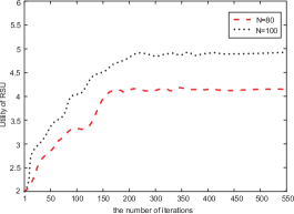
Figure 2: The convergence of utility of RSU with different number of users

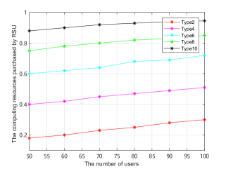
Figure 3: The computing resources purchased by RSU with different number of users

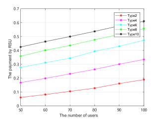
Figure 4: The payment by RSU with different number of users

With $e=e_{v}=a=60$, Fig. 2 shows the convergence of utility of RSU with different number of users, and demonstrates the convergence of Algorithm 2. Fig. 3 and Fig. 4 show the optimal contracts between the RSU and vehicles. As shown in Fig. 3, with the number of mobile device users rising, the computing resources that the RSU borrows from different types of vehicles also rise. Fig. 3 verifies Lemma 2, showing that the higher type a vehicle is, the more computing resources the RSU purchases. Fig. 4 shows that when the computing resources purchased by RSU increase, the expenses paid by RSU to each type of vehicles also increase. Fig. 4 demonstrates Lemma 1 as well, showing that the higher type a vehicle is, the more payment it gets.

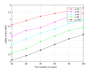
Figure 5: Utility of the RSU versus the number of users

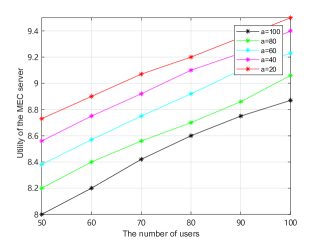
Figure 6: Utility of the MEC server versus the number of users

Fig. 5 and Fig. 6 reveal the relationship between the utility of RSU or MEC server and the number of users. Fixed the parameter $a$, it can be seen that with the number of users rising, the utility of RSU and MEC server also rises. However, when the number of users is fixed, with $a$ increasing, the utility of RSU and MEC server decreases.

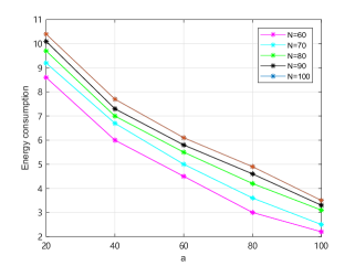
Figure 7: Energy consumption of MEC server versus energy cost coefficient $a$

Fig. 7 shows that, with $a$ increasing, the energy consumption of MEC server decreases. This means that the MEC server tends to use external resources. Fixed $a$, with the number of users rising, the energy consumption of MEC server also rises.

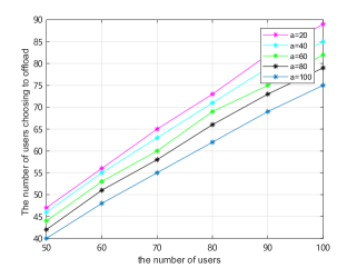
Figure 8: The number of users choosing to offload versus the total number of users

Fig. 8 shows the relationship between the number of users choosing to offload and the energy cost coefficient $a$. We can see that, fixed the number of users, when $a$ increases, since the energy consumption of MEC server decreases, users must pay more for computing resources and tend not to offload.

VI-C Comparative Study

TABLE II: Performance comparison between our mechanism vs pure MEC offloading [18], cloud-MEC collaborative offloading [19], and autonomous MEC offloading [24]

Compared Based On	Our Mechanism	Pure MEC Offloading	Cloud-MEC Collaborative Offloading	Autonomous MEC Offloading
Delay	low	medium	high	low
Energy Consumption	low	high	medium	low
Availability	almost always	within server’s range	always	always but not reliable
Cost	low	medium	high	low

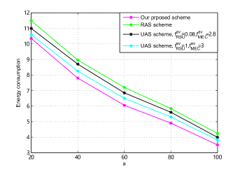
Figure 9: Energy consumption of MEC server in different schemes

First, we compare our approach with the existing schemes for vehicular MEC offloading. That is, the pure MEC offloading with dedicated MEC server in [18], the cloud-MEC collaborative computation offloading in [19], where an MEC server and a cloud server coexist, and the autonomous MEC offloading using neighbouring vehicles’ idle computing resources in [24]. In table II, we present the performance comparison between our proposed mechanism and the existing pure MEC offloading, cloud-MEC collaborative offloading and autonomous MEC offloading, which shows the advantages of our proposed mechanism in offloading delay, energy consumption and cost.

Then, we compare our proposed optimal computing resource allocation scheme with random allocation scheme (RAS) and uniform allocation scheme (UAS). Given $N=100$ users, RAS randomly allocates computing resources of the MEC server or vehicles, while in UAS, we have $f_{RSU}^{av}=\{0.08,0.1\}\mathrm{GHz},f_{MEC}^{av}=\{2.8,3\}\mathrm{GHz}$ for each user. As shown in Fig. 9, the energy consumption of MEC server in our scheme is lower than that in RAS and UAS schemes.

VII Conclusion

In this paper, we propose a vehicular fog-edge computing network for computation offloading. In order to portray this scene, we formulate it as a multi-stage Stackelberg game and a contract-based incentive mechanism. We solve this complex three-stage optimization problem by the backward induction method. Then we obtain the optimal price and computing resource demand strategies in each stage. Numerical results demonstrate the effectiveness of our proposed incentive mechanism and trading mechanism, reveal the trends of energy consumption and offloading decisions on various parameters, and show the performance comparison between our work and the other existing MEC offloading framework in vehicular networks. Our future work will include two aspects. First, based on HVC framework, combined with specific vehicle-to-everything applications (e.g., sensor data sharing and processing, use cases of automatic driving or advanced driving), the proposed algorithm will be verified with real objects. Besides, taking the heterogeneity of mobile device users and of vehicles, a finer-grained task assignment and resource scheduling algorithm will be studied.

Appendix

VII-A Proof of Proposition 1

Proof:

Obviously, the objective function of problem (18) is concave. Rewrite (18) as

$$\min_{p,f_{e},f_{RSU}} -\tau+\Delta p+k_{e}f_{e}^{2}+cf_{RSU}$$ (42)

$$\mathrm{s.t.}\ \mathbf{C6:} p\geq 0$$

$$\mathbf{C7:} 0\leq f_{e}\leq f_{e}^{\mathrm{max}}$$

$$\mathbf{C8:} f_{RSU}\geq 0$$

$$\mathbf{\overline{C9}:} \frac{\tau}{p}-\Delta=f_{e}+f_{RSU}$$

The Lagrangian function is defined as

$$\mathscr{L} =-\tau+\Delta p+k_{e}f_{e}^{2}+cf_{RSU}$$ (43)

$$+\alpha\left(\frac{\tau}{p}-\Delta-f_{e}-f_{RSU}\right)$$

$$+\gamma(f_{e}-f_{e}^{\mathrm{max}})-\zeta p-\xi f_{e}-\nu f_{RSU}.$$

According to the Karush-Kunh-Tucker (KKT) conditions, we have

$$\frac{\partial\mathscr{L}}{\partial p}=\Delta-\frac{\alpha\tau}{p^{2}}-\zeta=0,$$ (44)

$$\frac{\partial\mathscr{L}}{\partial f_{e}}=2k_{e}f_{e}-\alpha+\gamma-\xi=0,$$ (45)

$$\frac{\partial\mathscr{L}}{\partial f_{RSU}}=c-\alpha-\nu=0,$$ (46)

$$\frac{\tau}{p}-\Delta-f_{e}-f_{RSU}=0,$$ (47)

$$\gamma(f_{e}-f_{e}^{\mathrm{max}})=0,$$ (48)

$$\zeta p=0,\ \xi f_{e}=0,\ \nu f_{RSU}=0,$$ (49)

$$p,f_{e},f_{RSU},\alpha,\gamma,\zeta,\xi,\nu\geq 0.$$ (50)

Lemma 7

$\zeta=0$

Proof:

Suppose $\zeta\neq 0$. Since $\zeta p=0$, it follows that $p=0$. However, if $p=0$, then (47) does not hold. Thus, we have $\zeta=0$. ∎

Lemma 8

$\xi=0$

Proof:

Suppose $\xi\neq 0$. Similarly, we have $f_{e}=0$. If $f_{e}=0$, from (48) we know $\gamma=0$. From (45), we have $\alpha=-\xi$. Substituting $\alpha<0$ into $\frac{\partial\mathscr{L}}{\partial p}$, we can obtain that $\frac{\partial\mathscr{L}}{\partial p}>0$, which contradicts (44). Thus, $\xi=0$. ∎

Lemma 9

$\nu=0$

Proof:

Suppose $\nu\neq 0$. Then we have $f_{RSU}=0$. It means that the MEC server does not buy any computing resource from RSU. Therefore, the price of RSU’s resources is $c=0$. When $c=0$, from (46) we can obtain that $\alpha=-\nu<0$, which creates contradiction like Lemma 8. Thus, we have $\nu=0$. ∎

According to Lemma 7, 8 and 9, we can obtain the optimal solution of (42) by the KKT conditions easily. This problem is based on the assumption that all users choose to offload their tasks. Therefore, the price of MEC server’s computing resources must follow this condition:

$$p<\min\left\{\frac{\tau_{1}}{f_{1}^{l}\delta+f_{1}^{thresh}},\frac{\tau_{2}}{f_{2}^{l}\delta+f_{2}^{thresh}},\cdots,\frac{\tau_{N}}{f_{N}^{l}\delta+f_{N}^{thresh}}\right\},$$ (51)

From (17), we can reduce this condition to $p<\frac{\tau_{N}}{f_{N}^{l}\delta+f_{N}^{thresh}}$. Then, from (19), we have $\sqrt{\frac{c\sum_{i=1}^{N}\tau_{i}}{\delta\sum_{i=1}^{N}f_{i}^{l}}}<\frac{\tau_{N}}{f_{N}^{l}\delta+f_{N}^{thresh}}$. Thus, it follows that $c<T_{N}$. Then, the optimal solution of (18) can be solved. ∎

VII-B Proof of Proposition 2

Proof:

The sufficiency part has been proved in the proof of Proposition 1. Now we consider the necessity part. Suppose $T_{N}\leq c<T_{N-1}$, and the optimal price of MEC server’s computing resources is $p^{\star}$ given by (23). Since $c\geq T_{N}$, we have $p\geq\frac{\tau_{N}}{f_{N}^{l}\delta+f_{N}^{thresh}}$ and $f_{N}^{\star}=0$. Then (16) can be rewritten as

$$\max_{p,f_{e},f_{RSU}} \sum_{i=1}^{N-1}(\tau_{i}-f_{i}^{l}\delta p)-k_{e}f_{e}^{2}-cf_{RSU}$$ (52)

$$\mathrm{s.t.}\ \mathbf{C6} \mathbf{-C8}$$

$$\mathbf{\overline{C9}} \mathbf{:}\ \sum_{i=1}^{N-1}\left(\frac{\tau_{i}}{p}-f_{i}^{l}\delta\right)=f_{e}+f_{RSU}$$

This problem has the same structure as (18). Therefore, from the proof of the sufficiency part, we can see that the optimal price of MEC server’s computing resources for this problem is

$$p^{\star}=\sqrt{\frac{c\sum_{i=1}^{N-1}\tau_{i}}{\delta\sum_{i=1}^{N-1}f_{i}^{l}}}.$$ (53)

We can also obtain the optimal quantity of resources purchased by the MEC server from RSU.

Obviously, the optimal solution of (52) is different from that of (18). This contradicts with our presumption. Thus, $p^{\star}$ given by (19) is the optimal solution of (18) only if $c<T_{N}$. The necessity part is thus proved. ∎

VII-C Proof of Lemma 3

Proof:

According to IR conditions, we have

$$\theta_{1}p_{1}-k_{v}f_{1}^{2}\geq 0.$$ (54)

Due to IC conditions, we have

$$\theta_{m}p_{m}-k_{v}f_{m}^{2}\geq\theta_{m}p_{1}-k_{v}f_{1}^{2},\forall m\in\{2,3,\cdots,M\}.$$ (55)

As we know, $\theta_{1}\leq\theta_{2}\leq\cdots\leq\theta_{M}$, thus

$$\theta_{m}p_{m}-k_{v}f_{m}^{2}\geq\theta_{1}p_{1}-k_{v}f_{1}^{2}\geq 0,\forall m\in\{2,3,\cdots,M\}.$$ (56)

That is, if the IR condition of type-$1$ vehicles is satisfied, the other IR conditions also hold. ∎

VII-D Proof of Lemma 4

Proof:

According to IC conditions, we have

$$\theta_{m+1}p_{m+1}-k_{v}f_{m+1}^{2}\geq\theta_{m+1}p_{m}-k_{v}f_{m}^{2},$$ (57)

$$\theta_{m}p_{m}-k_{v}f_{m}^{2}\geq\theta_{m}p_{m-1}-k_{v}f_{m-1}^{2}.$$ (58)

According to Lemma 1 and 2, we have

$$\theta_{m+1}(p_{m}-p_{m-1})\geq\theta_{m}(p_{m}-p_{m-1}).$$ (59)

Combining (58) and (59), we get

$$\theta_{m+1}p_{m}-k_{v}f_{m}^{2}\geq\theta_{m+1}p_{m-1}-k_{v}f_{m-1}^{2}.$$ (60)

Combining (57) and (60), we get

$$\theta_{m+1}p_{m+1}-k_{v}f_{m+1}^{2}\geq\theta_{m+1}p_{m-1}-k_{v}f_{m-1}^{2}.$$ (61)

Recursively like this, we can prove Lemma 4. ∎

VII-E Proof of Lemma 5

Proof:

Assume that an LDIC constraint is not active, i.e., for type-$m$ vehicles,

$$\theta_{m}p_{m}-k_{v}f_{m}^{2}>\theta_{m}p_{m-1}-k_{v}f_{m-1}^{2}.$$ (62)

At this time, the RSU can gradually reduce the payment $p_{m}$ until both sides of (62) equal. This measure does not violate the LDIC constraints, but improves the utility of RSU. Therefore, under the optimal contract, all the LDIC constraints must be active.

Similarly, we can prove that the IR constraint of type-$1$ vehicles is active as well. ∎

VII-F Proof of Lemma 6

Proof:

According to Lemma 1, we have

$$\theta_{m}(p_{m}-p_{m-1})>\theta_{m-1}(p_{m}-p_{m-1}).$$ (63)

From Lemma 5, we get

$$k_{v}(f_{m}^{2}-f_{m-1}^{2})=\theta_{m}(p_{m}-p_{m-1}).$$ (64)

Then,

$$k_{v}(f_{m}^{2}-f_{m-1}^{2})>\theta_{m-1}(p_{m}-p_{m-1})$$ (65)

$$\Rightarrow \theta_{m-1}p_{m-1}-k_{v}f_{m-1}^{2}>\theta_{m-1}p_{m}-k_{v}f_{m}^{2},$$

i.e., the LUIC constraints hold. ∎

VII-G Proof of Theorem 2

Proof:

The first-order conditions of Lagrangian function (34) are

$$\frac{\partial\mathscr{L}}{\partial p_{m}}=\mu_{m+1}\theta_{m+1}-\mu_{m}\theta_{m}+l_{m}\theta_{m}=0,\ \forall m\in\{2,3,\cdots,M-1\},$$ (66)

$$\frac{\partial\mathscr{L}}{\partial p_{1}}=l_{1}\theta_{1}+\gamma\theta_{1}+\mu_{2}\theta_{2}=0,$$ (67)

$$\frac{\partial\mathscr{L}}{\partial p_{M}}=l_{M}\theta_{M}-\mu_{M}\theta_{M}=0.$$ (68)

Combining (66) and (68), we can obtain (35). From (67), we know that $\gamma=-\l_{1}-\mu_{2}\frac{\theta_{2}}{\theta_{1}}$.

$$\frac{\partial\mathscr{L}}{\partial f_{m}}=2k_{v}(\mu_{m}-\mu_{m+1})f_{m}-l_{m}\eta=0,\ \forall m\in\{2,3,\cdots,M-1\},$$ (69)

$$\frac{\partial\mathscr{L}}{\partial f_{1}}=-2k_{v}(\mu_{2}+\gamma)f_{1}-l_{1}\eta=0,$$ (70)

$$\frac{\partial\mathscr{L}}{\partial f_{M}}=2k_{v}\mu_{M}f_{M}-l_{M}\eta=0.$$ (71)

From (69), (70) and (71), we can obtain (37), (36) and (38).

According to the reduced IR constraint $\mathbf{\overline{C4}}$, the solution of $p_{1}$ can be written as (39). Then, given the solution $f_{i}^{\star},\ \forall i\in\{1,2,\cdots,M\}$ and the reduced IC constraints $\mathbf{\overline{C5}}$, we can get the optimal solution $p_{i}^{\star},\forall i\in\{1,2,\cdots,M\}$, which is shown in (40).

However, the analytical solution of $c$ can not be obtained directly. The gradient method can be used to update the Lagrangian multipliers to approximate to the optimal $c$, i.e.,

$$c^{(l)}=\left[c^{(l-1)}-\frac{\partial\mathscr{L}}{\partial c^{(l-1)}}\right]_{T_{k}}^{T_{k-1}}.$$ (72)

∎

References

- [1] C. Wang, Y. Li, D. Jin and S. Chen “On the Serviceability of Mobile Vehicular Cloudlets in a Large-Scale Urban Environment” In IEEE Transactions on Intelligent Transportation Systems 17.10, 2016, pp. 2960–2970 DOI: 10.1109/TITS.2016.2561293
- [2] R. Yu et al. “Optimal Resource Sharing in 5G-Enabled Vehicular Networks: A Matrix Game Approach” In IEEE Transactions on Vehicular Technology 65.10, 2016, pp. 7844–7856 DOI: 10.1109/TVT.2016.2536441
- [3] C. Shao et al. “Performance Analysis of Connectivity Probability and Connectivity-Aware MAC Protocol Design for Platoon-Based VANETs” In IEEE Transactions on Vehicular Technology 64.12, 2015, pp. 5596–5609 DOI: 10.1109/TVT.2015.2479942
- [4] K. Zhang et al. “Energy-Efficient Offloading for Mobile Edge Computing in 5G Heterogeneous Networks” In IEEE Access 4, 2016, pp. 5896–5907 DOI: 10.1109/ACCESS.2016.2597169
- [5] X. Hou et al. “Vehicular Fog Computing: A Viewpoint of Vehicles as the Infrastructures” In IEEE Transactions on Vehicular Technology 65.6, 2016, pp. 3860–3873 DOI: 10.1109/TVT.2016.2532863
- [6] W. Zhang et al. “Energy-Optimal Mobile Cloud Computing under Stochastic Wireless Channel” In IEEE Transactions on Wireless Communications 12.9, 2013, pp. 4569–4581 DOI: 10.1109/TWC.2013.072513.121842
- [7] S. Sardellitti, G. Scutari and S. Barbarossa “Joint Optimization of Radio and Computational Resources for Multicell Mobile-Edge Computing” In IEEE Transactions on Signal and Information Processing over Networks 1.2, 2015, pp. 89–103 DOI: 10.1109/TSIPN.2015.2448520
- [8] C. You, K. Huang, H. Chae and B. Kim “Energy-Efficient Resource Allocation for Mobile-Edge Computation Offloading” In IEEE Transactions on Wireless Communications 16.3, 2017, pp. 1397–1411 DOI: 10.1109/TWC.2016.2633522
- [9] Y. Dai, D. Xu, S. Maharjan and Y. Zhang “Joint Computation Offloading and User Association in Multi-Task Mobile Edge Computing” In IEEE Transactions on Vehicular Technology 67.12, 2018, pp. 12313–12325 DOI: 10.1109/TVT.2018.2876804
- [10] Y. Mao, J. Zhang and K.. Letaief “Dynamic Computation Offloading for Mobile-Edge Computing With Energy Harvesting Devices” In IEEE Journal on Selected Areas in Communications 34.12, 2016, pp. 3590–3605 DOI: 10.1109/JSAC.2016.2611964
- [11] J. Liu, Y. Mao, J. Zhang and K.. Letaief “Delay-optimal computation task scheduling for mobile-edge computing systems” In 2016 IEEE International Symposium on Information Theory (ISIT), 2016, pp. 1451–1455 DOI: 10.1109/ISIT.2016.7541539
- [12] C. Wang et al. “Joint Computation Offloading and Interference Management in Wireless Cellular Networks with Mobile Edge Computing” In IEEE Transactions on Vehicular Technology 66.8, 2017, pp. 7432–7445 DOI: 10.1109/TVT.2017.2672701
- [13] T.. Tran and D. Pompili “Joint Task Offloading and Resource Allocation for Multi-Server Mobile-Edge Computing Networks” In IEEE Transactions on Vehicular Technology 68.1, 2019, pp. 856–868 DOI: 10.1109/TVT.2018.2881191
- [14] T. Koketsu Rodrigues, K. Suto and N. Kato “Edge Cloud Server Deployment with Transmission Power Control through Machine Learning for 6G Internet of Things” In IEEE Transactions on Emerging Topics in Computing, 2019, pp. 1–1 DOI: 10.1109/TETC.2019.2963091
- [15] T.. Rodrigues et al. “Machine Learning Meets Computation and Communication Control in Evolving Edge and Cloud: Challenges and Future Perspective” In IEEE Communications Surveys Tutorials 22.1, 2020, pp. 38–67 DOI: 10.1109/COMST.2019.2943405
- [16] J. Liu et al. “A Scalable and Quick-Response Software Defined Vehicular Network Assisted by Mobile Edge Computing” In IEEE Communications Magazine 55.7, 2017, pp. 94–100 DOI: 10.1109/MCOM.2017.1601150
- [17] Lei Liu et al. “Vehicular Edge Computing and Networking: A Survey”, 2019 arXiv:1908.06849 [eess.SP]
- [18] V. Huy Hoang, T.. Ho and L.. Le “Mobility-Aware Computation Offloading in MEC-Based Vehicular Wireless Networks” In IEEE Communications Letters 24.2, 2020, pp. 466–469 DOI: 10.1109/LCOMM.2019.2956514
- [19] J. Zhao, Q. Li, Y. Gong and K. Zhang “Computation Offloading and Resource Allocation For Cloud Assisted Mobile Edge Computing in Vehicular Networks” In IEEE Transactions on Vehicular Technology 68.8, 2019, pp. 7944–7956 DOI: 10.1109/TVT.2019.2917890
- [20] H. Ke et al. “Deep Reinforcement Learning-Based Adaptive Computation Offloading for MEC in Heterogeneous Vehicular Networks” In IEEE Transactions on Vehicular Technology 69.7, 2020, pp. 7916–7929 DOI: 10.1109/TVT.2020.2993849
- [21] Z. Xiao et al. “Vehicular Task Offloading via Heat-Aware MEC Cooperation Using Game-Theoretic Method” In IEEE Internet of Things Journal 7.3, 2020, pp. 2038–2052 DOI: 10.1109/JIOT.2019.2960631
- [22] Y. Wang et al. “A Game-Based Computation Offloading Method in Vehicular Multiaccess Edge Computing Networks” In IEEE Internet of Things Journal 7.6, 2020, pp. 4987–4996 DOI: 10.1109/JIOT.2020.2972061
- [23] B. Gu and Z. Zhou “Task Offloading in Vehicular Mobile Edge Computing: A Matching-Theoretic Framework” In IEEE Vehicular Technology Magazine 14.3, 2019, pp. 100–106 DOI: 10.1109/MVT.2019.2902637
- [24] G. Qiao, S. Leng, K. Zhang and Y. He “Collaborative Task Offloading in Vehicular Edge Multi-Access Networks” In IEEE Communications Magazine 56.8, 2018, pp. 48–54 DOI: 10.1109/MCOM.2018.1701130
- [25] J. Feng, Z. Liu, C. Wu and Y. Ji “Mobile Edge Computing for the Internet of Vehicles: Offloading Framework and Job Scheduling” In IEEE Vehicular Technology Magazine 14.1, 2019, pp. 28–36 DOI: 10.1109/MVT.2018.2879647
- [26] Xiangwang Hou et al. “Reliable Computation Offloading for Edge-Computing-Enabled Software-Defined IoV” In IEEE Internet of Things Journal 7.8, 2020, pp. 7097–7111 DOI: 10.1109/JIOT.2020.2982292
- [27] Jinming Shi et al. “Priority-Aware Task Offloading in Vehicular Fog Computing Based on Deep Reinforcement Learning” In IEEE Transactions on Vehicular Technology 69.12, 2020, pp. 16067–16081 DOI: 10.1109/TVT.2020.3041929
- [28] F. Tang, Y. Kawamoto, N. Kato and J. Liu “Future Intelligent and Secure Vehicular Network Toward 6G: Machine-Learning Approaches” In Proceedings of the IEEE 108.2, 2020, pp. 292–307 DOI: 10.1109/JPROC.2019.2954595
- [29] F. Malandrino et al. “The Role of Parked Cars in Content Downloading for Vehicular Networks” In IEEE Transactions on Vehicular Technology 63.9, 2014, pp. 4606–4617 DOI: 10.1109/TVT.2014.2316645
- [30] Z. Su et al. “A Game Theoretic Approach to Parked Vehicle Assisted Content Delivery in Vehicular Ad Hoc Networks” In IEEE Transactions on Vehicular Technology 66.7, 2017, pp. 6461–6474 DOI: 10.1109/TVT.2016.2630300
- [31] G. Sun, M. Yu, D. Liao and V. Chang “Analytical Exploration of Energy Savings for Parked Vehicles to Enhance VANET Connectivity” In IEEE Transactions on Intelligent Transportation Systems 20.5, 2019, pp. 1749–1761 DOI: 10.1109/TITS.2018.2834569
- [32] Jyoti Grover “Vehicular fog computing paradigm: Scenarios and applications” In Vehicular Cloud Computing for Traffic Management and Systems IGI Global, 2018, pp. 200–215
- [33] X. Wang, Z. Ning and L. Wang “Offloading in Internet of Vehicles: A Fog-Enabled Real-Time Traffic Management System” In IEEE Transactions on Industrial Informatics 14.10, 2018, pp. 4568–4578 DOI: 10.1109/TII.2018.2816590
- [34] C. Li et al. “Parked Vehicular Computing for Energy-Efficient Internet of Vehicles: A Contract Theoretic Approach” In IEEE Internet of Things Journal 6.4, 2019, pp. 6079–6088 DOI: 10.1109/JIOT.2018.2869892
- [35] H. Sami, A. Mourad and W. El-Hajj “Vehicular-OBUs-As-On-Demand-Fogs: Resource and Context Aware Deployment of Containerized Micro-Services” In IEEE/ACM Transactions on Networking 28.2, 2020, pp. 778–790 DOI: 10.1109/TNET.2020.2973800
- [36] Z. Hou et al. “A contract-based incentive mechanism for energy harvesting-based Internet of Things” In 2017 IEEE International Conference on Communications (ICC), 2017, pp. 1–6 DOI: 10.1109/ICC.2017.7997316
- [37] B. Johansson, P. Soldati and M. Johansson “Mathematical decomposition techniques for distributed cross-layer optimization of data networks” In IEEE Journal on Selected Areas in Communications 24.8, 2006, pp. 1535–1547 DOI: 10.1109/JSAC.2006.879364
- [38] Dimitri P Bertsekas “Nonlinear programming” In Journal of the Operational Research Society 48.3 Taylor & Francis, 1997, pp. 334–334