Phase-field fracture irreversibility using the slack variable approach

Abstract

In this manuscript, the phase-field fracture irreversibility constraint is transformed into an equality-based constraint using the slack variable approach. The equality-based fracture irreversibility constraint is then introduced in the phase-field fracture energy functional using the Lagrange Multiplier Method and the Penalty method. Both methods are variationally consistent with the conventional variational inequality phase-field fracture problem, unlike the history-variable approach. Thereafter, numerical experiments are carried out on benchmark problems in brittle and quasi-brittle fracture to demonstrate the efficacy of the proposed method.

Highlights

• Effective equality constraint for fracture irreversibility inequality constraint using slack variable.

• The Lagrange Multiplier Method and the Penalty method are adopted to augment the energy functional.

• Numerical experiments carried out on both brittle and quasi-brittle fracture problems.

Keywords: phase-field fracture, brittle, quasi-brittle, Lagrange multiplier method, Penalty method, COMSOL

1 Introduction

The phase-field model for fracture emerged from the seminal work of [1], wherein the Griffith fracture criterion was cast into a variational setting. Later, a numerical implementation of the same was proposed in [2], using the Ambrosio–Tortorelli regularisation of the Mumford-Shah potential [3]. In this implementation, the fracture is represented by an auxiliary variable, that interpolates between the intact and broken material states. Such a formulation allows the automatic tracking of fractures on a fixed mesh, thereby eliminating the need for the tedious tracking and remeshing processes observed with discrete methods. Furthermore, the phase-field model for fracture is also able to handle topologically complex (branching, kinking and merging) fractures, and is able to demonstrate fracture initiation without introducing any singularity [4]. Owing to these advantages, the phase-field model for fracture has gained popularity in the computational mechanics community in the past decade.

A thermodynamically consistent formulation of the phase-field fracture model was proposed by [5], adopting an energetic cracking driving force definition. Since then, over the past decade, researchers have extended the work to thermo-mechanical problems at large strain [6], ductile failure [7, 8], fracture in thin films [9], anisotropic fracture [10], fracture in fully/partially saturated porous media [11, 12, 13], hydrogen assisted cracking [14], dissolution-driven stress corrosion cracking [15], fracture and fatigue in shape-memory alloys [16], and brittle failure of Reisner-Mindlin plates [17] to cite a few. Finally, the phase-field model for fracture has also been used for the multi-scale finite element method [18, 19, 20], asymptotic homogenisation [21], and variationally consistent homogenisation [22]. For a detailed overview on the phase-field fracture model, the reader is referred to the comprehensive review works [23, 24, 25].

Despite its growing popularity, the phase-field model for fracture poses several challenges when it comes to robust and computationally efficient solution techniques [25]. These include,

1. the poor performance of the monolithic Newton-Raphson (NR) method due to the non-convex energy functional,

2. variational inequality arising from fracture irreversibility, and

3. extremely fine meshes are required in the fracture zone.

In order to alleviate the problem concerning the poor-performance of the NR method (A), [26] utilised a linear extrapolation in time for the phase-field variable in the momentum balance equation. In [27], a novel line search technique was developed, while in [28] and [29] Augmented Lagrangian and modified NR approaches were proposed. More recently, [30] adopted a recursive multilevel trust region method, that resulted in improved convergence of the NR method. The development of robust, monolithic solution technique is still an active area in phase-field fracture research, and this manuscript is contribution towards this aspect.

The next issue pertains to the variational inequality problem arising out of the fracture irreversibility condition (B). This aspect has been treated in different ways in the phase-field fracture literature. They include crack set irreversibility [2, 31, 32], penalisation [4, 28, 29], and the implicit History variable based method proposed by [33]. The lattermost method remains popular despite its non-variational nature, over-estimation of the fracture surface energy, and the necessity for computationally expensive alternate minimisation (staggered) solution procedure [4]. In a novel approach, this manuscript adopts the slack variable method [34, 35], that constructs an equivalent variational equality problem, while maintaining the variational structure of the original problem.

Another issue pertaining to the phase-field fracture model is the requirement of extremely fine meshes in the smeared fracture zone (C). In this context, [2] and [9] advocates the use of uniformly refined meshes together with parallel computing while [36, 37, 38] opted for error-controlled adaptive mesh refinement. Some other approaches include pre-refined meshes when the fracture path is known [23, 27, 4], adaptive mesh refinement in [26] based on a phase-field threshold or Kelly error estimates [39], and multi-level hp-FEM in [40]. In this manuscript, uniformly refined meshes and pre-refined meshes based on a priori knowledge of the fracture path, are used.

The novelty of this manuscript lies in the alternative treatment of the fracture irreversibility inequality constraint, using the slack variable approach. The inequality constraint is replaced by an equivalent equality-based fracture irreversibility constraint. The constraint is then augmented to the phase-field fracture energy functional using the Lagrange Multiplier method and the Penalty method. These methods are variationally consistent, unlike the history-variable approach proposed in [33].

The manuscript is organised as follows: Section 2 introduces the phase-field model for fracture, its underlying energy functional and the Karush-Kuhn-Tucker (KKT) optimality conditions. Thereafter, in Section 3, the Method of Multipliers is adopted to augment the energy functional a slack variable-based fracture irreversibility criterion. The equivalence of the new formulation with the original problem in Section 2 is established in terms of KKT conditions. Furthermore, the Euler-Lagrange equations are presented. In Section 4, the slack variable-based fracture irreversibility constraint is introduced in the energy functional using the Penalisation method, followed by the derivation of the pertinent Euler-Lagrange equations. The numerical experiments on benchmark problems are presented in Section 5, and Section 6 lays down the concluding remarks of this manuscript.

Notation

The following notations are strictly adhered to in this manuscript:

• Zero-order tensors are represented using small italicized letters, e.g., $a$. Bold symbols are used for first and second-order tensors, for instance, stress $\sigma$ and strain $\epsilon$.

• A function $f$ with its arguments $x$, $y$ is written in the form $f(x,y)$, whereas a variable $g$ with operational dependencies $p,q$ is written as $g[p,q]$.

• The Macaulay operator on a variable $x$ is defined as $\langle x\rangle_{\pm}=\frac{1}{2}(x\pm|x|)$.

2 Phase-field fracture model

2.1 Energy functional

Let $\hbox{$\Omega$}\in\mathbb{R}^{\text{dim}}$ ($\text{dim}=2,3$) be the domain occupied by the fracturing solid, shown in Figure 1. Its boundary $\Gamma$ is decomposed into a Dirichlet boundary $\hbox{$\Gamma$}_{D}^{\scriptsize{u}}$ and a Neumann boundary $\hbox{$\Gamma$}_{N}^{\scriptsize{u}}$, such that $\hbox{$\Gamma$}=\hbox{$\hbox{$\Gamma$}_{D}^{\scriptsize{u}}$}\cup\hbox{$\hbox{$\Gamma$}_{N}^{\scriptsize{u}}$}$ and $\hbox{$\hbox{$\Gamma$}_{D}^{\scriptsize{u}}$}\cap\hbox{$\hbox{$\Gamma$}_{N}^{\scriptsize{u}}$}=\emptyset$. Furthermore, the fracture is represented by an auxiliary variable (phase-field) $\hbox{$\varphi$}\in[0,1]$ within a diffusive (smeared) zone of width $\hbox{$l$}>0$.

Figure 1: A solid $\hbox{$\Omega$}\in\mathbb{R}^{2}$ embedded with a diffused (smeared) crack. Dirichlet and Neumann boundaries are indicated with $\hbox{$\Gamma$}_{D}^{\scriptsize{u}}$ and $\hbox{$\Gamma$}_{N}^{\scriptsize{u}}$ respectively. Figure adopted from [22].

The energy functional of the phase-field fracture model [27, 4] is stated as,

$${}\displaystyle E(\hbox{$\mathbf{u}$},\hbox{$\varphi$})=\int_{\hbox{$\Omega$}}g(\hbox{$\varphi$})\Psi^{+}(\hbox{$\hbox{\boldmath$\epsilon$}$}[\hbox{$\mathbf{u}$}])\>\text{d}\hbox{$\Omega$}+\int_{\hbox{$\Omega$}}\Psi^{-}(\hbox{$\hbox{\boldmath$\epsilon$}$}[\hbox{$\mathbf{u}$}])\>\text{d}\hbox{$\Omega$}-\int_{\hbox{$\hbox{$\Gamma$}_{N}^{\scriptsize{u}}$}}\hbox{$\mathbf{t}_{p}^{\scriptsize{u}}$}\cdot\hbox{$\mathbf{u}$}\>\text{d}\hbox{$\Gamma$}+\int_{\hbox{$\Omega$}}\dfrac{\hbox{$G_{c}$}}{c_{w}\hbox{$l$}}\left(w(\hbox{$\varphi$})+\hbox{$l$}|\hbox{\boldmath$\nabla$}\hbox{$\varphi$}|^{2}\right)\>\text{d}\hbox{$\Omega$},$$ (1)

with $\mathbf{u}$ and $\varphi$ representing the displacement and the phase-field respectively. The symbols adopted for the additional functions and parameters in (1) are presented in Table 1.

Symbol	Function/Parameter
$g(\hbox{$\varphi$})$	Degradation function
$\Psi^{+}$	Fracture driving strain energy density
$\Psi^{-}$	Residual strain energy density
$\hbox{$\hbox{\boldmath$\epsilon$}$}[\hbox{$\mathbf{u}$}]$	Symmetric gradient of $\mathbf{u}$
$\mathbf{t}_{p}^{\scriptsize{u}}$	Prescribed traction
$G_{c}$	Griffith fracture energy
$c_{w}$	Normalisation constant
$l$	Fracture length-scale
$w(\hbox{$\varphi$})$	Local fracture energy function

Table 1: List of functions and parameters corresponding to the phase-field fracture energy functional (1).

In this manuscript, $\Psi^{+}$ and $\Psi^{-}$ represent the tensile and the compressive strain energy density functions respectively. They are functions of strain tensor $\hbox{$\hbox{\boldmath$\epsilon$}$}[\hbox{$\mathbf{u}$}]$, given by

$${}\hbox{$\hbox{\boldmath$\epsilon$}$}[\hbox{$\mathbf{u}$}]=(\hbox{$\mathbf{u}$}\otimes\hbox{\boldmath$\nabla$})^{\text{sym}}.$$ (2)

The explicit expression for $\Psi^{\pm}$ is obtained following [5] as,

$${}\Psi^{\pm}(\hbox{$\hbox{\boldmath$\epsilon$}$}[\hbox{$\mathbf{u}$}])=\frac{1}{2}\IfEqCase{1}{{1}{\lambda}{2}{\mu}}[]\langle(\mathbf{I}\colon\hbox{$\hbox{\boldmath$\epsilon$}$}[\hbox{$\mathbf{u}$}])\rangle^{2}_{\pm}+\IfEqCase{2}{{1}{\lambda}{2}{\mu}}[]\hbox{$\hbox{\boldmath$\epsilon$}$}^{\pm}[\hbox{$\mathbf{u}$}]\colon\hbox{$\hbox{\boldmath$\epsilon$}$}^{\pm}[\hbox{$\mathbf{u}$}],$$ (3)

where $\IfEqCase{1}{{1}{\lambda}{2}{\mu}}[]$ and $\IfEqCase{2}{{1}{\lambda}{2}{\mu}}[]$ are the Lamé constants, $\mathbf{I}$ is a second-order identity tensor, $\mathbf{u}$ is the displacement. Moreover, the tensile/compressive strain $\hbox{$\hbox{\boldmath$\epsilon$}$}^{\pm}[\hbox{$\mathbf{u}$}]$ is defined as

$$\hbox{$\hbox{\boldmath$\epsilon$}$}^{\pm}[\hbox{$\mathbf{u}$}]=\sum_{i=1}^{\text{dim}}\langle\epsilon_{i}\rangle_{\pm}\mathbf{p}_{i}\otimes\mathbf{p}_{i}$$ (4)

where $\epsilon_{i}$ represents the $i^{th}$ eigenvalue of the strain, and $\mathbf{p}_{i}$ is its corresponding normalised eigenvector. The tensile/compressive strain energy definition in (3) yield the corresponding stresses upon taking the derivative w.r.t the strain. They are explicitly stated in a compact form as,

$$\hbox{$\hbox{\boldmath$\sigma$}$}^{\pm}=\frac{\partial\Psi^{\pm}}{\partial\hbox{$\hbox{\boldmath$\epsilon$}$}}=\IfEqCase{1}{{1}{\lambda}{2}{\mu}}[]\langle(\mathbf{I}\colon\hbox{$\hbox{\boldmath$\epsilon$}$}[\hbox{$\mathbf{u}$}])\rangle_{\pm}\mathbf{I}+2\IfEqCase{2}{{1}{\lambda}{2}{\mu}}[]\hbox{$\hbox{\boldmath$\epsilon$}$}^{\pm}[\hbox{$\mathbf{u}$}].$$ (5)

The last integral in the energy functional (1) represents the fracture energy in a phase-field fracture model. The phase-field fracture model allows flexibility in the choice of the degradation function $g(\hbox{$\varphi$})$ and the locally dissipated fracture energy function $w(\hbox{$\varphi$})$. Table 2 presents commonly adopted functions for brittle and quasi-brittle fracture.

Model	$g(\hbox{$\varphi$})$	$w(\hbox{$\varphi$})$	$c_{w}$
Brittle-AT1[41]	$(1-\hbox{$\varphi$})^{2}$	$\varphi$	$8/3$
Brittle-AT2[31]	$(1-\hbox{$\varphi$})^{2}$	$\hbox{$\varphi$}^{2}$	$2$
Quasi-Brittle[42]	$\dfrac{(1-\hbox{$\varphi$})^{p}}{(1-\hbox{$\varphi$})^{p}+a_{1}\hbox{$\varphi$}+a_{1}a_{2}\hbox{$\varphi$}^{2}+a_{1}a_{2}a_{3}\hbox{$\varphi$}^{3}}$	$2\hbox{$\varphi$}-\hbox{$\varphi$}^{2}$	$\pi$

Table 2: Degradation function, local fracture energy function and its normalisation constant for different phase-field fracture models. The abbreviation ‘AT’ stands for Ambrosio-Tortorelli.

For the Quasi-Brittle model in Table 2, the parameters $p$, $a_{1}$, $a_{2}$ and $a_{3}$ are chosen such that they mimic the different traction-separation laws in cohesive zone modelling. Following [42], the constant $a_{1}$ is given by

$$a_{1}=\dfrac{4E_{0}\hbox{$G_{c}$}}{\pi\hbox{$l$}f_{t}^{2}}$$ (6)

where, the newly introduced parameters $E_{0}$ and $f_{t}$ represent the Youngs’ modulus and the tensile strength of the material. Next, Table 3 presents the different traction-separation laws and the corresponding values of $p$, $a_{2}$ and $a_{3}$ [42].

Model	$p$	$a_{2}$	$a_{3}$
Linear Softening	$2$	$-0.5$	$0$
Exponential Softening	$2.5$	$2^{5/3}-3$	$0$
Cornelissen et. al.[43] Softening	$2$	$1.3868$	$0.6567$

Table 3: Quasi-brittle phase-field fracture models and their parameters, based on [42].

The prediction of fracture initiation and propagation in the solid occupying the domain $\Omega$ requires solving the constrained minimisation problem:

Problem 1.

Find $\hbox{$\mathbf{u}$}(t)$ and $\hbox{$\varphi$}(t)$, where ${}^{n}\hbox{$\varphi$}=\hbox{$\varphi$}(t_{n})$ is known for $t_{n}<t$ such that,

$$\begin{array}[]{lll}min_{\tiny{\hbox{$\mathbf{u}$}(t),\hbox{$\varphi$}(t)}}E&\text{and}&h(\hbox{$\varphi$})\geq 0,\end{array}$$ (7)

where $h(\hbox{$\varphi$})=\hbox{$\varphi$}-{}^{n}\hbox{$\varphi$}$, and the left superscript $n$ denotes the previous time-step. Moreover, the problem is augmented with (pseudo) time-dependent Dirichlet boundary conditions $\hbox{$\mathbf{u}$}^{p}$ on $\hbox{$\Gamma$}_{D}^{\scriptsize{u}}$ and $\hbox{$\varphi$}^{p}$ on $\hbox{$\Gamma$}_{D}^{\scriptsize{\hbox{$\varphi$}}}$, and/or Neumann boundary conditions $\mathbf{t}_{p}^{\scriptsize{u}}$ on $\hbox{$\Gamma$}_{N}^{\scriptsize{u}}$ and $\mathbf{t}_{p}^{\scriptsize{\hbox{$\varphi$}}}$ on $\hbox{$\Gamma$}_{N}^{\scriptsize{\hbox{$\varphi$}}}$. Furthermore, the boundary $\Gamma$ is split as $\hbox{$\Gamma$}=\hbox{$\hbox{$\Gamma$}_{D}^{\scriptsize{u}}$}\cup\hbox{$\hbox{$\Gamma$}_{N}^{\scriptsize{u}}$}$, $\hbox{$\hbox{$\Gamma$}_{D}^{\scriptsize{u}}$}\cap\hbox{$\hbox{$\Gamma$}_{N}^{\scriptsize{u}}$}=\emptyset$ and $\hbox{$\Gamma$}=\hbox{$\hbox{$\Gamma$}_{D}^{\scriptsize{\hbox{$\varphi$}}}$}\cup\hbox{$\hbox{$\Gamma$}_{N}^{\scriptsize{\hbox{$\varphi$}}}$}$, $\hbox{$\hbox{$\Gamma$}_{D}^{\scriptsize{\hbox{$\varphi$}}}$}\cap\hbox{$\hbox{$\Gamma$}_{N}^{\scriptsize{\hbox{$\varphi$}}}$}=\emptyset$ respectively. $\blacksquare$

2.2 Karush-Kuhn-Tucker conditions

The KKT triple ($\hbox{$\mathbf{u}$},\hbox{$\varphi$},\Lambda$) in appropriate spaces for the Problem 1 requires

$$\big{[}E(\hbox{$\mathbf{u}$},\hbox{$\varphi$})-\int_{\hbox{$\Omega$}}\Lambda h(\hbox{$\varphi$})\,\text{d}\hbox{$\Omega$}\big{]}^{\prime}_{\hbox{$\mathbf{u}$}} =0,$$ (8a)

$$\big{[}E(\hbox{$\mathbf{u}$},\hbox{$\varphi$})-\int_{\hbox{$\Omega$}}\Lambda h(\hbox{$\varphi$})\,\text{d}\hbox{$\Omega$}\big{]}^{\prime}_{\hbox{$\varphi$}} =0,,$$ (8b)

$$h(\hbox{$\varphi$}) \geq 0,$$ (8c)

$$\Lambda \geq 0,$$ (8d)

$$\Lambda h(\hbox{$\varphi$}) =0$$ (8e)

to hold, where $\Lambda$ is a multiplier. Equations (8a) and (8b) represent the Euler-Lagrange equations pertaining to the stationary condition, while equations (8c-8e) are the primal and dual feasibility conditions, and the complementary slackness respectively. Formally, the latter set of equations enforces fracture irreversbility. To the same end, alternative, but equivalent formulations have been adopted in the phase-field fracture literature. For instance, [26] adopted the primal-dual active set strategy proposed by [44], [28] utilised an Augmented Lagrangian penalisation approach with the Moreau-Yoshida indicator function, and [4] opted for a simple penalisation approach. The authors would like to emphasise that the rather popular history-variable approach in [5] is not variationally consistent.

3 Lagrange Multiplier Method (LMM)

3.1 Fracture irreversibility and modified energy functional

In order to enforce fracture irreversibility $h(\hbox{$\varphi$})=\hbox{$\varphi$}-{}^{n}\hbox{$\varphi$}\geq 0$, a slack variable is defined as

$$\hbox{$\theta$}^{2}=h(\hbox{$\varphi$})=\hbox{$\varphi$}-{}^{n}\hbox{$\varphi$}.$$ (9)

It is observed that $\hbox{$\theta$}^{2}$ admits value greater than or equal to zero, thereby fulfilling the fracture irreversibility criterion. Next, the constrained minimisation Problem 1 is reformulated as:

Problem 2.

Find $\hbox{$\mathbf{u}$}(t)$, $\hbox{$\varphi$}(t)$ and $\hbox{$\theta$}(t)$ such that,

$$\begin{array}[]{lll}\text{min}_{\scriptsize{\hbox{$\mathbf{u}$}(t),\hbox{$\varphi$}(t)},\hbox{$\theta$}(t)}\>\>E\\ \text{subjected to}\>\>h(\hbox{$\varphi$})-\hbox{$\theta$}^{2}=0.\end{array}$$ (10)

with suitable (pseudo) time-dependent Dirichlet and/or Neumann boundary conditions, as mentioned in Problem 1. $\blacksquare$

Augmenting the equality constraint (10) in (1) via the Lagrange multiplier $\Lambda$ results in the modified energy functional,

$${}\tilde{E}(\hbox{$\mathbf{u}$},\hbox{$\varphi$},\theta,\Lambda)=E(\hbox{$\mathbf{u}$},\hbox{$\varphi$})-\Lambda\big{(}h(\hbox{$\varphi$})-\hbox{$\theta$}^{2}\big{)}.$$ (11)

3.2 Stationary conditions

The stationary conditions for the Problem 2 are given by

$$\tilde{E}^{\prime}_{\hbox{$\mathbf{u}$}}(\hbox{$\mathbf{u}$},\hbox{$\varphi$},\hbox{$\theta$},\Lambda;\hbox{$\delta\mathbf{u}$}) =0,$$ (12a)

$$\tilde{E}^{\prime}_{\hbox{$\varphi$}}(\hbox{$\mathbf{u}$},\hbox{$\varphi$},\hbox{$\theta$},\Lambda;\hbox{$\delta\varphi$}) =0,$$ (12b)

$$\tilde{E}^{\prime}_{\hbox{$\theta$}}(\hbox{$\mathbf{u}$},\hbox{$\varphi$},\hbox{$\theta$},\Lambda;\delta\hbox{$\theta$}) =0,$$ (12c)

$$\tilde{E}^{\prime}_{\Lambda}(\hbox{$\mathbf{u}$},\hbox{$\varphi$},\hbox{$\theta$},\Lambda;\delta\Lambda) =0.$$ (12d)

For equivalence of these conditions with those presented for Problem 1, the reader is referred to Proposition 3.1 in [45].

3.3 Euler-Lagrange equations

The Euler-Lagrange equations for Problem 2 are (12a)-(12d), obtained upon taking the first variation of the energy functional (11) w.r.t its solution variables $\mathbf{u}$, $\varphi$, $\theta$ and $\Lambda$. This results in,

Problem 3.

Find ($\mathbf{u}$, $\varphi$, $\theta$, $\Lambda$) $\in\mathbb{U}\times\mathbb{V}\times\mathbb{W}\times\mathbb{A}$ with

$$R^{\mathbf{u}} =\int_{\hbox{$\Omega$}}\bigg{(}g(\hbox{$\varphi$})\hbox{$\hbox{\boldmath$\sigma$}^{+}$}[\hbox{$\mathbf{u}$}]+\hbox{$\hbox{\boldmath$\sigma$}^{-}$}[\hbox{$\mathbf{u}$}]\bigg{)}\colon\hbox{$\hbox{\boldmath$\epsilon$}$}[\hbox{$\delta\mathbf{u}$}]\>\text{d}\hbox{$\Omega$}=0\>\>\> \forall\>\hbox{$\delta\mathbf{u}$}\in\mathbb{U}^{0}$$ (13a)

$$R^{\varphi} =\int_{\hbox{$\Omega$}}\bigg{(}\dfrac{\hbox{$G_{c}$}}{c_{w}\hbox{$l$}}w^{\prime}(\hbox{$\varphi$})+g^{\prime}(\hbox{$\varphi$})\Psi^{+}(\hbox{$\hbox{\boldmath$\epsilon$}$}[\hbox{$\mathbf{u}$}])-\Lambda\bigg{)}\hbox{$\delta\varphi$}\>\text{d}\hbox{$\Omega$}+\int_{\hbox{$\Omega$}}\dfrac{2\hbox{$G_{c}$}\hbox{$l$}}{c_{w}}\hbox{\boldmath$\nabla$}\hbox{$\varphi$}\cdot\hbox{\boldmath$\nabla$}\hbox{$\delta\varphi$}\>\text{d}\hbox{$\Omega$}=0\>\>\> \forall\>\hbox{$\delta\varphi$}\in\mathbb{V}^{0}$$ (13b)

$$R^{\theta} =\int_{\hbox{$\Omega$}}2\Lambda\theta\delta\theta\>\text{d}\hbox{$\Omega$}=0\>\>\> \forall\>\delta\theta\in\mathbb{W}$$ (13c)

$$R^{\Lambda} =-\int_{\hbox{$\Omega$}}\big{(}h(\hbox{$\varphi$})-\hbox{$\theta$}^{2}\big{)}\delta\Lambda\>\text{d}\hbox{$\Omega$}=0\>\>\> \forall\>\delta\Lambda\in\mathbb{A}.$$ (13d)

with trial function spaces

$$\mathbb{U}:=\{\hbox{$\mathbf{u}$}\in[H^{1}(\hbox{$\Omega$})]^{\text{dim}}|\hbox{$\mathbf{u}$}=\hbox{$\mathbf{u}$}^{\text{{p}}}\>\>\text{on}\>\>\hbox{$\hbox{$\Gamma$}_{D}^{\scriptsize{u}}$}\},$$ (14a)

$$\mathbb{V}:=\{\hbox{$\varphi$}\in[H^{1}(\hbox{$\Omega$})]^{1}|\hbox{$\varphi$}=\hbox{$\varphi$}^{\text{{p}}}\>\>\text{on}\>\>\hbox{$\hbox{$\Gamma$}_{D}^{\scriptsize{\hbox{$\varphi$}}}$}\},$$ (14b)

$$\mathbb{W}:=\{\theta\in[L_{2}(\hbox{$\Omega$})]\},$$ (14c)

$$\mathbb{A}:=\{\Lambda\in[L_{2}(\hbox{$\Omega$})]\},$$ (14d)

and test function spaces

$$\mathbb{U}^{0}:=\{\hbox{$\mathbf{u}$}\in[H^{1}(\hbox{$\Omega$})]^{\text{dim}}|\hbox{$\mathbf{u}$}=0\>\>\text{on}\>\>\hbox{$\hbox{$\Gamma$}_{D}^{\scriptsize{u}}$}\},$$ (15a)

$$\mathbb{V}^{0}:=\{\hbox{$\varphi$}\in[H^{1}(\hbox{$\Omega$})]^{1}|\hbox{$\varphi$}=0\>\>\text{on}\>\>\hbox{$\hbox{$\Gamma$}_{D}^{\scriptsize{\hbox{$\varphi$}}}$}\},$$ (15b)

and pertinent (pseudo) time-dependent Neumann condition

$$\mathbf{t}:=\left(g(\hbox{$\varphi$})\hbox{$\hbox{\boldmath$\sigma$}^{+}$}+\hbox{$\hbox{\boldmath$\sigma$}^{-}$}\right)\cdot\mathbf{n}=\hbox{$\mathbf{t}_{p}^{\scriptsize{u}}$}\>\>\text{on}\>\>\hbox{$\hbox{$\Gamma$}_{N}^{\scriptsize{u}}$}.$$ (16)

$\blacksquare$

Remark 1.

In the event $\Lambda$ and $\theta$ are zero, their stiffness contribution is zero and the stiffness matrix is singular. In order to avoid this situation a fictitious stiffness is introduced to guarantee solvability.

4 Penalty (Pen.) method

4.1 The energy functional

In an alternative approach, the squared slack variable equation (9) is introduced in the energy functional (1) as a quadratic term via penalisation. This results in the modified energy functional,

$${}\hat{E}(\hbox{$\mathbf{u}$},\hbox{$\varphi$},\theta)=E(\hbox{$\mathbf{u}$},\hbox{$\varphi$})+\dfrac{\eta}{2}\int_{\hbox{$\Omega$}}\bigg{(}h(\hbox{$\varphi$})-\hbox{$\theta$}^{2}\bigg{)}^{2}\,\text{d}\hbox{$\Omega$},$$ (17)

where, $\eta$ is a penalty parameter.

4.2 Euler-Lagrange equations

The Euler-Lagrange equations are obtained upon taking the first variation of the energy functional (17) w.r.t its solution variables $\mathbf{u}$, $\varphi$ and $\theta$. This results in:

Problem 4.

Find ($\mathbf{u}$, $\varphi$, $\theta$) $\in\mathbb{U}\times\mathbb{V}\times\mathbb{W}$ with

$$R^{\mathbf{u}} =\int_{\hbox{$\Omega$}}\bigg{(}g(\hbox{$\varphi$})\hbox{$\hbox{\boldmath$\sigma$}^{+}$}[\hbox{$\mathbf{u}$}]+\hbox{$\hbox{\boldmath$\sigma$}^{-}$}[\hbox{$\mathbf{u}$}]\bigg{)}\colon\hbox{$\hbox{\boldmath$\epsilon$}$}[\hbox{$\delta\mathbf{u}$}]\>\text{d}\hbox{$\Omega$}=0\>\>\> \forall\>\hbox{$\delta\mathbf{u}$}\in\mathbb{U}^{0}$$ (18a)

$$R^{\varphi} =\int_{\hbox{$\Omega$}}\bigg{(}\dfrac{\hbox{$G_{c}$}}{c_{w}\hbox{$l$}}w^{\prime}(\hbox{$\varphi$})+g^{\prime}(\hbox{$\varphi$})\Psi^{+}(\hbox{$\hbox{\boldmath$\epsilon$}$}[\hbox{$\mathbf{u}$}])+\eta(h(\hbox{$\varphi$})-\hbox{$\theta$}^{2})\bigg{)}\hbox{$\delta\varphi$}\>\text{d}\hbox{$\Omega$}+\int_{\hbox{$\Omega$}}\dfrac{2\hbox{$G_{c}$}\hbox{$l$}}{c_{w}}\hbox{\boldmath$\nabla$}\hbox{$\varphi$}\cdot\hbox{\boldmath$\nabla$}\hbox{$\delta\varphi$}\>\text{d}\hbox{$\Omega$}=0\>\>\> \forall\>\hbox{$\delta\varphi$}\in\mathbb{V}^{0}$$ (18b)

$$R^{\theta} =\int_{\hbox{$\Omega$}}-2\eta\theta(h(\hbox{$\varphi$})-\hbox{$\theta$}^{2})\delta\theta\>\text{d}\hbox{$\Omega$}=0\>\>\> \forall\>\delta\theta\in\mathbb{W}$$ (18c)

with trial function spaces

$$\mathbb{U}:=\{\hbox{$\mathbf{u}$}\in[H^{1}(\hbox{$\Omega$})]^{\text{dim}}|\hbox{$\mathbf{u}$}=\hbox{$\mathbf{u}$}^{\text{{p}}}\>\>\text{on}\>\>\hbox{$\hbox{$\Gamma$}_{D}^{\scriptsize{u}}$}\},$$ (19a)

$$\mathbb{V}:=\{\hbox{$\varphi$}\in[H^{1}(\hbox{$\Omega$})]^{1}|\hbox{$\varphi$}=\hbox{$\varphi$}^{\text{{p}}}\>\>\text{on}\>\>\hbox{$\hbox{$\Gamma$}_{D}^{\scriptsize{\hbox{$\varphi$}}}$}\},$$ (19b)

$$\mathbb{W}:=\{\theta\in[L_{2}(\hbox{$\Omega$})]|\},$$ (19c)

and test function spaces

$$\mathbb{U}^{0}:=\{\hbox{$\mathbf{u}$}\in[H^{1}(\hbox{$\Omega$})]^{\text{dim}}|\hbox{$\mathbf{u}$}=0\>\>\text{on}\>\>\hbox{$\hbox{$\Gamma$}_{D}^{\scriptsize{u}}$}\},$$ (20a)

$$\mathbb{V}^{0}:=\{\hbox{$\varphi$}\in[H^{1}(\hbox{$\Omega$})]^{1}|\hbox{$\varphi$}=0\>\>\text{on}\>\>\hbox{$\hbox{$\Gamma$}_{D}^{\scriptsize{\hbox{$\varphi$}}}$}\},$$ (20b)

and pertinent (pseudo) time-dependent Neumann condition

$$\mathbf{t}:=\left(g(\hbox{$\varphi$})\hbox{$\hbox{\boldmath$\sigma$}^{+}$}+\hbox{$\hbox{\boldmath$\sigma$}^{-}$}\right)\cdot\mathbf{n}=\hbox{$\mathbf{t}_{p}^{\scriptsize{u}}$}\>\>\text{on}\>\>\hbox{$\hbox{$\Gamma$}_{N}^{\scriptsize{u}}$}.$$ (21)

$\blacksquare$

Remark 2.

In the event $h(\hbox{$\varphi$})-\hbox{$\theta$}^{2}$ and $\theta$ are zero, their stiffness contribution is zero and the stiffness matrix is singular. In order to avoid this situation a fictitious stiffness is introduced to guarantee solvability.

5 Numerical Study

The numerical experiments on benchmark problems are presented in this section. They include both brittle and quasi-brittle fracture. In the brittle fracture domain, the Single Edge Notched Specimen under Tension (SENT), and under Shear (SENS), and the Notched concrete specimen with a hole [23] is presented. For quasi-brittle fracture, the benchmark problems include the concrete three-point bending problem [46], and the Winkler L-shaped panel experiment [47]. For each problem, the geometry as well as the material properties and loading conditions are presented in the respective sub-section. The load-displacement curves and the phase-field topology at the final step of analysis is also presented.

For the penalty method, the penalty parameter $\eta$ is set to $10^{6}$ [N/mm²] throughout the study. This choice is motivated by similarity of the load-displacement curves obtained with those from the Lagrange Multiplier Method. Furthermore, for both the aforementioned methods, a fully coupled monolithic solution technique is adopted using the Newton-Raphson solver in COMSOL Multiphysics. The iterations are terminated when the error measure defined as the weighted Euclidean norm of the solution update,

$$err:=\sqrt{\dfrac{1}{M}}\sqrt{\sum_{j=1}^{M}\dfrac{1}{N_{j}}\sum_{i=1}^{N}\bigg{(}\dfrac{|E_{i,j}|}{W_{i,j}}\bigg{)}^{2}},$$ (22)

is less than $1e-4$. In the above equation, $M$ indicates the number of fields, $j$ is the number of degree of freedom for each field $j=1,2,..M$, $E$ represents the absolute update (say, $\hbox{$\mathbf{u}$}^{(m)}$-${\hbox{$\mathbf{u}$}}^{(m-1)}$ for displacement, $m$ being the iteration count), and $W_{i,j}=max(|\mathbf{U}_{i,j}|,S_{j})$. The entire solution vector is represented with $\mathbf{U}$ and $S_{j}$ refers to scaling of solution variables.

5.1 Brittle: Single Edge Notched specimen under Tension (SENT)

A unit square (in mm) embedded with a horizontal notch, midway along the height is considered, as shown in Figure 3. The length of the notch (shown in red) is equal to half of the edge length of the plate. The notch is modelled explicitly in the finite element mesh. A quasi-static loading is applied at the top boundary in the form of prescribed displacement increment $\Delta\hbox{$u$}=1e-5$[mm] for the first $450$ steps, following which it is changed to $1e-6$[mm]. Furthermore, the bottom boundary remains fixed. The additional model parameters are presented in Table 4.

Figure 2: SENT experiment

Figure 3: SENS experiment

Parameters	Value
Model	Brittle-AT2
$\lambda$	121.154 [GPa]
$\mu$	80.769 [GPa]
$G_{c}$	2700 [N/m]
$l$	1.5e-2 [mm]
Element size	$\hbox{$l$}/2$

Table 4: Parameters

(a)

(b)

Figure 4: Figure (a) presents the load-displacement curves for the single edge notched specimen under tension. Here, LMM and Pen. refer to the Lagrange Multiplier Method and the Penalty method respectively. Figure (b) shows the distribution of the phase-field variable at the final step of the analysis.

Figure 4(a) presents the load-displacement curves obtained using the Lagrange Multiplier Method (LMM) and Penalty (Pen.) method, along with those from the literature [5, 23]. Both methods yield a similar behaviour compared to [5], in terms of the peak load and the post-peak behaviour. Moreover, the phase-field fracture topology at failure in Figure 4(b) is also identical to those reported in the aforementioned literature.

5.2 Brittle: Single Edge Notched specimen under Shear (SENS)

In order to perform a shear test, the SEN specimen is loaded horizontally along the top edge as shown in Figure 3. The material properties remain same as presented in Table 4. A quasi-static loading is applied to the top boundary in the form of prescribed displacement increment $\Delta\hbox{$u$}=1e-4$[mm] for the first $90$ steps, following which it is changed to $1e-5$[mm]. Furthermore, the bottom boundary remains fixed, and roller support is implemented in left and right edges thereby restricting the vertical displacement.

Figure 5(a) presents the load-displacement curves obtained using the Lagrange Multiplier Method and the Penalty method, along with those from the literature [5]. The former methods result in  $9\%$ higher peak load estimation as compared to [5]. However, the phase-field fracture topology in the final step of the analysis is consistent with those reported in the aforementioned literature.

(a)

(b)

Figure 5: Figure (a) presents the load-displacement curves for the single edge notched specimen under shear. Here, LMM and Pen. refer to the Lagrange Multiplier Method and the Penalty method respectively. Figure (b) shows the distribution of the phase-field variable at the final step of the analysis.

5.3 Brittle: Notched concrete specimen with a hole

A notched concrete specimen with a hole, shown in Figure 7 is considered in this study. The experimental and numerical analysis of the same has been carried out earlier in [23]. The specimen has dimensions 65 x 120 [mm²], the hole being 20 [mm] in diameter located at (36.5 [mm], 51[mm]). Moreover, a notch, 10 [mm] in length is located at 65 [mm] height from the bottom of the plate. The model parameters used in the simulation is presented in Table 5, while the experimentally observed fracture pattern is shown in Figure 7. As shown in Figure 7, the plate is loaded via the upper pin (in grey) with displacement increment $\Delta\hbox{$u$}=1e-3$ mm, while the lower pin (in grey) is remains fixed.

Figure 6: Geometry and constraints

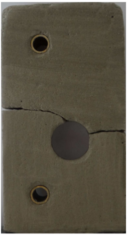
Figure 7: Experimental results [23]

Symbol	Value
Model	Brittle-AT2
$\lambda$	1.94 [kN/mm2]
$\mu$	2.45 [kN/mm2]
$G_{c}$	2.28e-3 [kN/mm]
$l$	0.25 [mm]
Element size	$\hbox{$l$}/2$

Table 5: Material properties [48]

Figure 8(a) presents the load-displacement curves obtained using the Lagrange Multiplier Method and the Penalty method, along with those from the literature [23, 48]. The curves corresponding to the Lagrange Multiplier Method and the Penalty method coincide, and predict peak loads close to those obtained in [23] and [48]. However, the load-displacement curves are significantly different from [23]. The reason for this behaviour is not investigated in this manuscript. However, it is important to note that in this work, the upper and lower pins are assumed to be rigid connectors. As such, the loading or fixed boundary conditions is applied w.r.t. the centre of the pin. Furthermore, [23] opted for $\hbox{$l$}=0.1$ [mm], in this manuscript as well as in [48], $\hbox{$l$}=0.25$ [mm]. Finally, from Figure 8(b), it observed that the final phase-field fracture topology does match the experimentally observed fracture patterns in Figure 7.

(a)

(b)

Figure 8: Figure (a) presents the load-displacement curves for the notched specimen with hole test, obtained from the current implementation, [23], and [48]. Here, LMM and Pen. refer to the Lagrange Multiplier Method and the Penalty method respectively. Figure (b) shows the distribution of the phase-field variable at the final step of the analysis in a section of the specimen.

5.4 Quasi-brittle: Concrete three-point bending

A three-point bending experiment on a notched concrete beam reported in [46] is considered here. The beam has dimensions $450\times 100$ [mm²], and has a notch $5\times 50$ [mm²]. A schematic of the beam along with the loading conditions is presented in Figure 9. Displacement-based load increments of $\Delta\hbox{$u$}=1e-3$ [mm] is enforced throughout the simulation. The model parameters are presented in Table 6.

Figure 9: Three point bending test

Parameters	Value
Model	Quasi-brittle
Softening	Cornellisen et. al. [43]
$E_{0}$	2e4 [MPa]
$\nu$	0.2 [-]
$f_{t}$	2.4 [MPa]
$G_{c}$	0.113 [N/mm]
$l$	2.5 [mm]
Element size	$\hbox{$l$}/5$

Table 6: Parameters for three point bending test

Figure 10(a) presents the load-displacement curves obtained using the Lagrange Multiplier Method and the Penalty method, along with those obtained from the experiments [46]. It is observed that both methods yield identical curves. These curves are close to the experimental upper bound (shaded region). Furthermore, the phase-field fracture topology at the final step in the analysis in Figure 10(b) is also identical to that reported in [46].

(a) Load-displacement plot

(b)

Figure 10: Figure (a) presents the load-displacement curves for the concrete three-point bending test. Here, LMM and Pen. refer to the Lagrange Multiplier Method and the Penalty method respectively. The experimental range is represented by the shaded area. Figure (b) shows the distribution of the phase-field variable at the final step of the analysis in a section of the beam.

5.5 Quasi-brittle: Winkler L-panel

The L-shaped panel studied by [47, 49] is considered in this sub-section. Figure 11 shows the geometry as well as the loading conditions. The longer edges of the panel are 500 [mm] and the smaller edges are 250 [mm]. The loading is applied on the edge marked in blue, 30 [mm] in length, and is in the form of displacement-based increments of $\Delta\hbox{$u$}=1e-3$ [mm]. The additional model parameters are presented in Table 7.

Figure 11: Winkler L-panel

Parameters	Value
Model	Quasi-brittle
Softening	Cornellisen et. al. [43]
$E_{0}$	2.0e4 [MPa]
$\nu$	0.18 [-]
$f_{t}$	2.5 [MPa]
$G_{c}$	0.130 [N/mm]
$l$	5 [mm]
Element size	$\hbox{$l$}/5$

Table 7: Parameters for L-shaped panel test [49]

(a) Load-displacement plot

(b)

Figure 12: Figure (a) presents the load-displacement curves for the concrete Winkler L-panel test. Here, LMM and Pen. refer to the Lagrange Multiplier Method and the Penalty method respectively. The experimental range is represented by the shaded area. Figure (b) shows the distribution of the phase-field variable at the final step of the analysis in a section of the beam.

Figure 12(a) presents the load-displacement curves obtained using the Lagrange Multiplier Method and the Penalty method, along with those obtained from the experiments [47, 49]. It is observed that the curves obtained using both methods are identical. These curves are also close to the experimental range (shaded region). Furthermore, the phase-field fracture topology at the final step in the analysis in Figure 12(b) is also identical to that reported in [47, 49].

6 Concluding Remarks

An alternative treatment of the phase-field fracture irreversibility constraint is presented in this manuscript. The fracture irreversibility constraint $h(\hbox{$\varphi$})\geq 0$ is transformed into an equivalent equality constraint. This is carried out upon introducing a slack variable $\theta$, and equating $h(\hbox{$\varphi$})$ to $\theta^{2}$. By definition, $\theta^{2}$ admits zero or positive values, thereby ensuring the fracture irreversibility constraint. The constraint is then introduced in the phase-field fracture energy functional using the Lagrange Multiplier Method and the Penalty method. The slack variable approach preserves the variational nature of the phase-field fracture problem, unlike the history variable approach in [33]. Furthermore, numerical experiments are conducted on benchmark brittle (AT2) and quasi-brittle fracture problems to demonstrate the efficacy of the proposed methods.

The scope for future studies include the extension towards complex multi-physics problems, large-scale problems, that maybe require special preconditioning techniques. Other future research directions may be towards accelerating the convergence rate using Anderson acceleration [50] or Large time increment method [51, 52].

7 Software Implementation and Data Availability

The numerical study in Section 5 is carried out using the equation-based modelling approach in the software package COMSOL Multiphysics 5.6. The source files would be made available in Github repository of the corresponding author (https://github.com/rbharali/PhaseFieldFractureCOMSOL/).

References

- [1] G.A. Francfort and J.-J. Marigo “Revisiting brittle fracture as an energy minimization problem” In Journal of the Mechanics and Physics of Solids 46.8, 1998, pp. 1319–1342 DOI: 10.1016/S0022-5096(98)00034-9
- [2] B. Bourdin, G.A. Francfort and J-J. Marigo “Numerical experiments in revisited brittle fracture” In Journal of the Mechanics and Physics of Solids 48.4, 2000, pp. 797–826 DOI: https://doi.org/10.1016/S0022-5096(99)00028-9
- [3] David Mumford and Jayant Shah “Optimal approximations by piecewise smooth functions and associated variational problems” In Communications on Pure and Applied Mathematics 42.5, 1989, pp. 577–685 DOI: 10.1002/cpa.3160420503
- [4] T. Gerasimov and L. De Lorenzis “On penalization in variational phase-field models of brittle fracture” In Computer Methods in Applied Mechanics and Engineering 354, 2019, pp. 990–1026 DOI: https://doi.org/10.1016/j.cma.2019.05.038
- [5] C. Miehe, F. Welschinger and M. Hofacker “Thermodynamically consistent phase-field models of fracture: Variational principles and multi-field FE implementations” In International Journal for Numerical Methods in Engineering 83.10, 2010, pp. 1273–1311 DOI: 10.1002/nme.2861
- [6] Christian Miehe, Lisa Marie Schänzel and Heike Ulmer “Phase field modeling of fracture in multi-physics problems. Part I. Balance of crack surface and failure criteria for brittle crack propagation in thermo-elastic solids” In Computer Methods in Applied Mechanics and Engineering 294, 2015, pp. 449–485 DOI: 10.1016/j.cma.2014.11.016
- [7] C. Miehe, M. Hofacker, L.. Schänzel and F. Aldakheel “Phase field modeling of fracture in multi-physics problems. Part II. Coupled brittle-to-ductile failure criteria and crack propagation in thermo-elastic-plastic solids” In Computer Methods in Applied Mechanics and Engineering 294, 2015, pp. 486–522 DOI: 10.1016/j.cma.2014.11.017
- [8] M. Ambati, T. Gerasimov and L. De Lorenzis “Phase-field modeling of ductile fracture” In Computational Mechanics 55.5, 2015, pp. 1017–1040 DOI: 10.1007/s00466-015-1151-4
- [9] A. Mesgarnejad, B. Bourdin and M.M. Khonsari “A variational approach to the fracture of brittle thin films subject to out-of-plane loading” In Journal of the Mechanics and Physics of Solids 61.11, 2013, pp. 2360–2379 DOI: https://doi.org/10.1016/j.jmps.2013.05.001
- [10] Thanh Tung Nguyen, Julien Réthoré and Marie-Christine Baietto “Phase field modelling of anisotropic crack propagation” In European Journal of Mechanics - A/Solids 65, 2017, pp. 279–288 DOI: https://doi.org/10.1016/j.euromechsol.2017.05.002
- [11] Christian Miehe and Steffen Mauthe “Phase field modeling of fracture in multi-physics problems. Part III. Crack driving forces in hydro-poro-elasticity and hydraulic fracturing of fluid-saturated porous media” In Computer Methods in Applied Mechanics and Engineering 304 Elsevier B.V., 2016, pp. 619–655 DOI: 10.1016/j.cma.2015.09.021
- [12] T. Cajuhi, L. Sanavia and L. De Lorenzis “Phase-field modeling of fracture in variably saturated porous media” In Computational Mechanics 61.3 Springer Berlin Heidelberg, 2018, pp. 299–318 DOI: 10.1007/s00466-017-1459-3
- [13] A. Mikelić, M.. Wheeler and T. Wick “Phase-field modeling through iterative splitting of hydraulic fractures in a poroelastic medium” In GEM - International Journal on Geomathematics 10 Springer International Publishing, 2019 DOI: 10.1007/s13137-019-0113-y
- [14] Emilio Martínez-Pañeda, Alireza Golahmar and Christian F. Niordson “A phase field formulation for hydrogen assisted cracking” In Computer Methods in Applied Mechanics and Engineering 342, 2018, pp. 742–761 DOI: 10.1016/j.cma.2018.07.021
- [15] Chuanjie Cui, Rujin Ma and Emilio Martínez-Pañeda “A phase field formulation for dissolution-driven stress corrosion cracking” In Journal of the Mechanics and Physics of Solids 147, 2021, pp. 104254 DOI: https://doi.org/10.1016/j.jmps.2020.104254
- [16] Marlini Simoes and Emilio Martínez-Pañeda “Phase field modelling of fracture and fatigue in Shape Memory Alloys” In Computer Methods in Applied Mechanics and Engineering 373, 2021, pp. 113504 DOI: https://doi.org/10.1016/j.cma.2020.113504
- [17] G. Kikis, M. Ambati, L. De Lorenzis and S. Klinkel “Phase-field model of brittle fracture in Reissner–Mindlin plates and shells” In Computer Methods in Applied Mechanics and Engineering 373, 2021, pp. 113490 DOI: https://doi.org/10.1016/j.cma.2020.113490
- [18] R.U. Patil, B.K. Mishra and I.V. Singh “An adaptive multiscale phase field method for brittle fracture” In Computer Methods in Applied Mechanics and Engineering 329, 2018, pp. 254–288 DOI: 10.1016/j.cma.2017.09.021
- [19] R.U. Patil, B.K. Mishra, I.V. Singh and T.Q. Bui “A new multiscale phase field method to simulate failure in composites” In Advances in Engineering Software 126, 2018, pp. 9–33 DOI: https://doi.org/10.1016/j.advengsoft.2018.08.010
- [20] R.U. Patil, B.K. Mishra and I.V. Singh “A multiscale framework based on phase field method and XFEM to simulate fracture in highly heterogeneous materials” In Theoretical and Applied Fracture Mechanics 100, 2019, pp. 390–415 DOI: https://doi.org/10.1016/j.tafmec.2019.02.002
- [21] F. Fantoni, A. Bacigalupo, M. Paggi and J. Reinoso “A phase field approach for damage propagation in periodic microstructured materials” In International Journal of Fracture, 2019 DOI: 10.1007/s10704-019-00400-x
- [22] Ritukesh Bharali, Fredrik Larsson and Ralf Jänicke “Computational homogenisation of phase-field fracture” In European Journal of Mechanics - A/Solids 88, 2021, pp. 104247 DOI: https://doi.org/10.1016/j.euromechsol.2021.104247
- [23] Marreddy Ambati, Tymofiy Gerasimov and Laura De Lorenzis “A review on phase-field models of brittle fracture and a new fast hybrid formulation” In Computational Mechanics 55.2, 2014, pp. 383–405 DOI: 10.1007/s00466-014-1109-y
- [24] Jian-Ying Wu et al. “Chapter One - Phase-field modeling of fracture” 53, Advances in Applied Mechanics Elsevier, 2020, pp. 1–183 DOI: https://doi.org/10.1016/bs.aams.2019.08.001
- [25] Laura De Lorenzis and Tymofiy Gerasimov “Numerical implementation of phase-field models of brittle fracture” In Modeling in Engineering Using Innovative Numerical Methods for Solids and Fluids Springer, 2020, pp. 75–101
- [26] Timo Heister, Mary F. Wheeler and Thomas Wick “A primal-dual active set method and predictor-corrector mesh adaptivity for computing fracture propagation using a phase-field approach” In Computer Methods in Applied Mechanics and Engineering, 2015 DOI: 10.1016/j.cma.2015.03.009
- [27] T. Gerasimov and L. De Lorenzis “A line search assisted monolithic approach for phase-field computing of brittle fracture” In Computer Methods in Applied Mechanics and Engineering 312, 2016, pp. 276–303 DOI: 10.1016/j.cma.2015.12.017
- [28] Thomas Wick “An Error-Oriented Newton/Inexact Augmented Lagrangian Approach for Fully Monolithic Phase-Field Fracture Propagation” In SIAM Journal on Scientific Computing 39.4, 2017, pp. B589–B617 DOI: 10.1137/16m1063873
- [29] Thomas Wick “Modified Newton methods for solving fully monolithic phase-field quasi-static brittle fracture propagation” In Computer Methods in Applied Mechanics and Engineering, 2017 DOI: 10.1016/j.cma.2017.07.026
- [30] Alena Kopaničáková and Rolf Krause “A recursive multilevel trust region method with application to fully monolithic phase-field models of brittle fracture” In Computer Methods in Applied Mechanics and Engineering 360, 2020, pp. 112720 DOI: https://doi.org/10.1016/j.cma.2019.112720
- [31] B. Bourdin “Numerical implementation of the variational formulation for quasi-static brittle fracture” In Interfaces and Free Boundaries 9, 2007, pp. 411–430 DOI: 10.4171/IFB/171
- [32] Siobhan Burke, Christoph Ortner and Endre Süli “An Adaptive Finite Element Approximation of a Variational Model of Brittle Fracture” In SIAM Journal on Numerical Analysis 48.3, 2010, pp. 980–1012 DOI: 10.1137/080741033
- [33] Christian Miehe, Martina Hofacker and Fabian Welschinger “A phase field model for rate-independent crack propagation: Robust algorithmic implementation based on operator splits” In Computer Methods in Applied Mechanics and Engineering 199.45-48 Elsevier B.V., 2010, pp. 2765–2778 DOI: 10.1016/j.cma.2010.04.011
- [34] FA Valentine “The problem of Lagrange with differentiable inequality as added side conditions. 407–448” In Contributions to the Calculus of Variations 37, 1933
- [35] D P Bertsekas “Nonlinear Programming” In Journal of the Operational Research Society 48.3 Taylor & Francis, 1997, pp. 334–334 DOI: 10.1057/palgrave.jors.2600425
- [36] Siobhan Burke, Christoph Ortner and Endre Süli “An adaptive finite element approximation of a variational model of brittle fracture” In SIAM Journal on Numerical Analysis 48.3 SIAM, 2010, pp. 980–1012
- [37] Marco Artina, Massimo Fornasier, Stefano Micheletti and Simona Perotto “Anisotropic mesh adaptation for crack detection in brittle materials” In SIAM Journal on Scientific Computing 37.4 SIAM, 2015, pp. B633–B659
- [38] Thomas Wick “Goal functional evaluations for phase-field fracture using PU-based DWR mesh adaptivity” In Computational Mechanics 57.6 Springer, 2016, pp. 1017–1035
- [39] D.. Kelly, J.. De S.., O.. Zienkiewicz and I. Babuska “A posteriori error analysis and adaptive processes in the finite element method: Part I—error analysis” In International Journal for Numerical Methods in Engineering 19.11, 1983, pp. 1593–1619 DOI: https://doi.org/10.1002/nme.1620191103
- [40] S. Nagaraja et al. “Phase-field modeling of brittle fracture with multi-level hp-FEM and the finite cell method” In Computational Mechanics 63.6, 2019, pp. 1283–1300 DOI: 10.1007/s00466-018-1649-7
- [41] Kim Pham, Hanen Amor, Jean-Jacques Marigo and Corrado Maurini “Gradient damage models and their use to approximate brittle fracture” In International Journal of Damage Mechanics 20.4 SAGE Publications Sage UK: London, England, 2011, pp. 618–652
- [42] Jian-Ying Wu “A unified phase-field theory for the mechanics of damage and quasi-brittle failure” In Journal of the Mechanics and Physics of Solids 103 Elsevier, 2017, pp. 72–99
- [43] H Cornelissen, D Hordijk and H Reinhardt “Experimental determination of crack softening characteristics of normalweight and lightweight” In Heron 31.2, 1986, pp. 45–46
- [44] M. Hintermüller, K. Ito and K. Kunisch “The Primal-Dual Active Set Strategy as a Semismooth Newton Method” In SIAM Journal on Optimization 13.3, 2002, pp. 865–888 DOI: 10.1137/S1052623401383558
- [45] R.. Tapia “A stable approach to Newton’s method for general mathematical programming problems inRn” In Journal of Optimization Theory and Applications 14.5, 1974, pp. 453–476 DOI: 10.1007/BF00932842
- [46] Jan Rots “Computational modeling of concrete fracture”, 1988
- [47] Bernhard Josef Winkler “Traglastuntersuchungen von unbewehrten und bewehrten Betonstrukturen auf der Grundlage eines objektiven Werkstoffgesetzes für Beton” Innsbruck University Press, 2001
- [48] Yousef Navidtehrani, Covadonga Betegón and Emilio Martínez-Pañeda “A Unified Abaqus Implementation of the Phase Field Fracture Method Using Only a User Material Subroutine” In Materials 14.8, 2021 DOI: 10.3390/ma14081913
- [49] Jörg F Unger, Stefan Eckardt and Carsten Könke “Modelling of cohesive crack growth in concrete structures with the extended finite element method” In Computer methods in applied mechanics and engineering 196.41-44 Elsevier, 2007, pp. 4087–4100
- [50] Donald G Anderson “Iterative procedures for nonlinear integral equations” In Journal of the ACM (JACM) 12.4 ACM New York, NY, USA, 1965, pp. 547–560
- [51] Dan Givoli, Ritukesh Bharali and Lambertus J Sluys “LATIN: A new view and an extension to wave propagation in nonlinear media” In International Journal for Numerical Methods in Engineering 112.2 Wiley Online Library, 2017, pp. 125–156
- [52] Ritukesh Bharali “An Adaptive Generic Incremental LATIN method”, 2017