Fast Sinkhorn I: an $O(N)$ algorithm for the Wasserstein-1 metric

Abstract

The Wasserstein metric is broadly used in optimal transport for comparing two probabilistic distributions, with successful applications in various fields such as machine learning, signal processing, seismic inversion, etc. Nevertheless, the high computational complexity is an obstacle for its practical applications. The Sinkhorn algorithm, one of the main methods in computing the Wasserstein metric, solves an entropy regularized minimizing problem, which allows arbitrary approximations to the Wasserstein metric with $O(N^{2})$ computational cost. However, higher accuracy of its numerical approximation requires more Sinkhorn iterations with repeated matrix-vector multiplications, which is still unaffordable. In this work, we propose an efficient implementation of the Sinkhorn algorithm to calculate the Wasserstein-1 metric with $O(N)$ computational cost, which achieves the optimal theoretical complexity. By utilizing the special structure of Sinkhorn’s kernel, the repeated matrix-vector multiplications can be implemented with $O(N)$ times multiplications and additions, using the Qin Jiushao or Horner’s method for efficient polynomial evaluation, leading to an efficient algorithm without losing accuracy. In addition, the log-domain stabilization technique, used to stabilize the iterative procedure, can also be applied in this algorithm. Our numerical experiments show that the newly developed algorithm is one to three orders of magnitude faster than the original Sinkhorn algorithm.

49M25; 49M30; 65K10

1 Introduction

The Wasserstein metric has been widely used in optimal transport for the global comparison between probabilistic distributions. It has been successfully used in various fields such as machine learning [17, 28], image processing [38], inverse problems [8, 14, 33, 51, 19], and density function theory[21, 7, 12]. Many numerical methods have been developed, including the linear programming methods [36, 26, 50], combinatorial methods [42], solving Monge-Amphère equations [16, 15, 5, 4] and proximal splitting methods [11, 34]. In recent years, several approximation techniques in optimal transport for high-dimensional distributions have also been proposed approximately [31, 32].

One of the popular numerical techniques to compute the Wasserstein metric, is the the Sinkhorn algorithm [13, 45], which minimizes the entropy regularized problem. It provides the solution roughly in $O(N^{2})$ operations with guaranteed convergence [29]. With the help of GPU acceleration, the efficiency of using the Sinkhorn algorithm to solve the optimal transport problem can be more significantly improved [25, 40, 41]. For the Wasserstein-2 matric, the computation can be accelerated using the Gaussian convolution by approximating the geodesic distance-based kernel with the heat kernel [46]. Moreover, through statistical sampling, dimensional reduction, and other approximation methods, the complexity of the Sinkhorn algorithm can be reduced to $O(N\log N)$ [2, 23] or even $O(N)$ [43]. An alternative way is to define the Wasserstein metric on the finite tree space, and the computational complexity could be $O(N\log N)$ [24, 47]. Because of these progresses, the Sinkhorn algorithm has been widely used in practical problems. However, those techniques provide just approximations of the transportation cost, rather than the precise computation of the original optimization problem. Therefore, it is still of great interest to develop fast and accurate Sinkhorn-type algorithms for solving large-scale optimal transport problems.

In recent years, some fast algorithms for accurately solving the optimal transport problem have been developed recently. For example, through multi-level grids, the computation complexity can be reduced to $O(N^{1.5}\log N)$ [30]. Another well-known conclusion is that for the one-dimensional quadratic Wasserstein metric, the complexity of the sorting-based algorithm is only $O(N\log N)$ [37].

In this work, by observing the special structure of the kernel matrix in the Sinkhorn algorithm to solve the Wasserstein-1 metric, we propose a novel matrix-vector multiplication based on dynamic programming [22]. During each iteration step, it involves only a forward and backward recursive sweeping process, as in Qin Jiushao’s (or Horners’, although it appeared several centuries later) method for polynomial evaluations [35, 20], which reduces the computational cost from $O(N^{2})$ to $O(N)$ in each step, thus achieving the optimal theoretical complexity. In addition, the log-stabilization [9], an important technique to improve the numerical stability of the Sinkhorn algorithm, can be implemented in this strategy with the same stability property. In this paper we abbreviate this method as FS-1.

The rest of the paper is organized as follows. In Section 2, the basics of the Wasserstein-1 metric and the Sinkhorn algorithm are briefly introduced. After showing the elaborate structure of the obtained kernel matrix, we use it to develop the FS-1 algorithm in Section 3. We will also analyze the stability and integrate the log-stabilization technique into our FS-1 to improve the numerical stability. In Section 4, the FS-1 is generalized to higher dimension. We will provide numerical experiments to illustrate the huge efficiency advantage of our FS-1 algorithm in Section 5. Finally, we conclude the paper in Section 6.

2 The Wasserstein-1 metric and the Sinkhorn algorithm

Consider two probabilistic density functions $u(x)$ and $v(x)$ on a doman $\Omega\subset\mathbb{R}$, the Kantorovich’s formulation of Wasserstein-1 metric is defined as [48]:

$$\begin{split}W(u,v)&=\inf_{\gamma(x,y)\in\Gamma}\int_{\Omega\times\Omega}d(x,y)\gamma(x,y)\mathrm{d}x\mathrm{d}y,\\ \Gamma=\Big{\{}\gamma(x,y)\Big{|}&\int_{\Omega}\gamma(x,y)\mathrm{d}y=u(x),\int_{\Omega}\gamma(x,y)\mathrm{d}x=v(y)\Big{\}},\end{split}$$ (2.1)

where $d(x,y)=|x-y|$. The Sinkhorn algorithm proposed in [13, 45] introduces an entropy term and solves the regularized problem:

$$W_{\varepsilon}(u,v)=\inf_{\gamma(x,y)\in\Gamma}\int_{\Omega\times\Omega}\left|x-y\right|\gamma(x,y)+\varepsilon\gamma(x,y)\ln\big{(}\gamma(x,y)\big{)}\mathrm{d}x\mathrm{d}y.$$ (2.2)

As for numerical realization, we consider two discretized probabilistic distributions

$$\boldsymbol{u}=(u_{1},u_{2},\cdots u_{N}),\quad\boldsymbol{v}=(v_{1},v_{2},\cdots,v_{N}),$$

on a uniform mesh grid with a grid spacing of $h$. Then the entropy regularized minimizing problem (2.2) can be discretized as

$$W_{\varepsilon}(\boldsymbol{u},\boldsymbol{v})=\inf_{\gamma_{ij}}\sum_{i=1}^{N}\sum_{j=1}^{N}\left(\gamma_{ij}\left|i-j\right|h+\varepsilon\gamma_{ij}\ln\big{(}\gamma_{ij}\big{)}\right),$$ (2.3)

and $\gamma_{ij}$ satisfies

$$\sum_{j=1}^{N}\gamma_{ij}=u_{i},\quad\sum_{i=1}^{N}\gamma_{ij}=v_{j},\quad\gamma_{ij}\geq 0.$$

The Lagrangian of the above equations writes

$$L(\boldsymbol{\gamma},\boldsymbol{\alpha},\boldsymbol{\beta})=\sum_{i=1}^{N}\sum_{j=1}^{N}\left(\gamma_{ij}\left|i-j\right|h+\varepsilon\gamma_{ij}\ln(\gamma_{ij})\right)+\sum_{i=1}^{N}\alpha_{i}(\sum_{j=1}^{N}\gamma_{ij}-u_{i})+\sum_{j=1}^{N}\beta_{j}(\sum_{i=1}^{N}\gamma_{ij}-v_{j}).$$

Taking the derivative of the Lagrangian with respect of $\gamma_{ij}$ directly leads to

$$\gamma_{ij}=e^{-\frac{1}{2}-\frac{1}{\varepsilon}\alpha_{i}}K_{ij}e^{-\frac{1}{2}-\frac{1}{\varepsilon}\beta_{j}},\;\;\textrm{where}\;\;K_{ij}=e^{-\left|i-j\right|h/\varepsilon}.$$

To avoid $\varepsilon$ in the denominator, set $\phi_{i}=e^{-\frac{1}{2}-\frac{1}{\varepsilon}\alpha_{i}}$ and $\psi_{j}=e^{-\frac{1}{2}-\frac{1}{\varepsilon}\beta_{j}}$, we obtain

$$\phi_{i}\sum_{j=1}^{N}K_{ij}\psi_{j}=u_{i},\quad\psi_{j}\sum_{i=1}^{N}K_{ij}\phi_{i}=v_{j},\quad\forall i,\;j=1,2,\cdots,N.$$

Since the entries in $K=(K_{ij})$ are strictly positive, Sinkhorn’s iteration [45] can be applied to iteratively update vectors $\boldsymbol{\phi}=(\phi_{i})$ and $\boldsymbol{\psi}=(\psi_{j})$ by pointwise computation:

$$\boldsymbol{\psi}^{(\ell+1)}=\boldsymbol{v}\oslash(K^{T}\boldsymbol{\phi}^{(\ell)}),\quad\boldsymbol{\phi}^{(\ell+1)}=\boldsymbol{u}\oslash(K\boldsymbol{\psi}^{(\ell+1)}),$$ (2.4)

in which the notion $\oslash$ represents pointwise division and $\ell$ denotes the iterative steps.

Remark 2.1.

In [9], a log-domain stabilization technique is proposed to reduce the numerical instability caused by the small parameter $\varepsilon$. The idea is that when the infinite norms of $\boldsymbol{\phi}$ or $\boldsymbol{\psi}$ exceed a given threshold $\tau$, these two vectors will be normalized with the excessive part ‘absorbed’ in $\boldsymbol{\alpha}$ and $\boldsymbol{\beta}$:

$$\boldsymbol{\alpha}\leftarrow\boldsymbol{\alpha}+\ln(\boldsymbol{\phi}^{(\ell)}),\quad\boldsymbol{\beta}\leftarrow\boldsymbol{\beta}+\ln(\boldsymbol{\psi}^{(\ell)}),\quad\boldsymbol{\phi}^{(\ell)}\leftarrow\mathbf{1}_{N},\quad\boldsymbol{\psi}^{(\ell)}\leftarrow\mathbf{1}_{N}.$$

Correspondingly, the matrix $K$ needs to be rescaled as $K\leftarrow diag(e^{\boldsymbol{\alpha}/\varepsilon})\times K\times diag(e^{\boldsymbol{\beta}/\varepsilon}).$

3 The FS-1 Algorithm

The key to the Sinkhorn algorithm is to iteratively update $\boldsymbol{\phi}$ and $\boldsymbol{\psi}$ through equation (2.4). By introducing the notation $\lambda=e^{-h/\varepsilon}$, the matrix multiplication vector operation is written as

$$K\boldsymbol{\psi}^{(\ell)}=\begin{pmatrix}\psi^{(\ell)}_{1}&+&\lambda\psi^{(\ell)}_{2}&+&\lambda^{2}\psi^{(\ell)}_{3}&\cdots&+&\lambda^{N-1}\psi^{(\ell)}_{N}\\ \lambda\psi^{(\ell)}_{1}&+&\psi^{(\ell)}_{2}&+&\lambda\psi^{(\ell)}_{3}&\cdots&+&\lambda^{N-2}\psi^{(\ell)}_{N}\\ \lambda^{2}\psi^{(\ell)}_{1}&+&\lambda\psi^{(\ell)}_{2}&+&\psi^{(\ell)}_{3}&\cdots&+&\lambda^{N-3}\psi^{(\ell)}_{N}\\ \vdots&\vdots&\vdots&\vdots&\vdots&\ddots&\vdots&\vdots\\ \lambda^{N-1}\psi^{(\ell)}_{1}&+&\lambda^{N-2}\psi^{(\ell)}_{2}&+&\lambda^{N-3}\psi^{(\ell)}_{3}&\cdots&+&\psi^{(\ell)}_{N}\end{pmatrix}.$$ (3.5)

We separate the summation of row $k$ to the lower triangular part $p_{k}$ and the strictly upper triangular part $q_{k}$. Then updating $\boldsymbol{\phi}^{(\ell+1)}$ is formulated as

$$\phi^{(\ell+1)}_{k}=u_{k}/(p_{k}+q_{k}),\quad p_{k}=\sum_{i=1}^{k}\psi^{(\ell)}_{i}\lambda^{k-i},\quad q_{k}=\sum_{i=k+1}^{N}\psi^{(\ell)}_{i}\lambda^{i-k},\quad k=1,2,\cdots,N.$$

Instead of directly calculating $p_{k}$ and $q_{k}$, we use the recursive computation given by

$$p_{1}=\psi^{(\ell)}_{1},\quad p_{k+1}=\lambda p_{k}+\psi^{(\ell)}_{k+1},\quad k=1,2,\cdots,N-1,$$ (3.6)

$$q_{N}=0,\quad q_{k}=\lambda(q_{k+1}+\psi^{(\ell)}_{k+1}),\quad k=N-1,N-2,\cdots,1.$$

This is the Qin Jiushao or Horner method for efficient polynomial evaluation [35, 20]. Thus we develop the FS-1 algorithm with linear computational complexity, which only takes $2(N-1)$ times additions and multiplications for the matrix multiplication operation. The pseudo-code is presented in Algorithm 1.

Algorithm 1 FS-1 Algorithm

Input: $\boldsymbol{u}$ and $\boldsymbol{v}$ of size $(N,1)$, $h$, $\varepsilon$, $\mathrm{tol}$, $\mathrm{itr\_max}$
  Output: $W_{\varepsilon}(\boldsymbol{u},\boldsymbol{v})$

1:$\lambda=e^{-h/\varepsilon}$; $\boldsymbol{\phi}^{(0)},\boldsymbol{\psi}^{(0)}=\frac{1}{N}\mathbf{1}_{N}$; $\boldsymbol{p}^{(0)},\boldsymbol{r}^{(0)},\boldsymbol{q}^{(0)},\boldsymbol{s}^{(0)}=\mathbf{0}_{N}$; $\ \ell=0$

2:while $\left(\ell\;<\;\mathrm{itr\_max}\right)$ and $\left(\sum_{i=1}^{N}\left|\psi_{i}^{(\ell)}(\sum_{j=1}^{N}\phi_{j}^{(\ell)}\lambda^{\left|i-j\right|})-v_{i}\right|\;>\;\mathrm{tol}\right)$ do

3:     $r^{(\ell)}_{1}=\phi^{(\ell)}_{1}$, $s^{(\ell)}_{N}=0$

4:     for $i=1\;:\;N-1$ do

5:         $r^{(\ell)}_{i+1}=\lambda r^{(\ell)}_{i}+\phi^{(\ell)}_{i+1}$

6:         $s^{(\ell)}_{N-i}=\lambda(s^{(\ell)}_{N-i+1}+\phi^{(\ell)}_{N-i+1})$      

7:     $\boldsymbol{\psi}^{(\ell+1)}=\boldsymbol{v}\oslash\left(\boldsymbol{r}^{(\ell)}+\boldsymbol{s}^{(\ell)}\right)$

8:     $p^{(\ell)}_{1}=\psi^{(\ell+1)}_{1}$, $q^{(\ell)}_{N}=0$

9:     for $i=1\;:\;N-1$ do

10:         $p^{(\ell)}_{i+1}=\lambda p^{(\ell)}_{i}+\psi^{(\ell+1)}_{i+1}$

11:         $q^{(\ell)}_{N-i}=\lambda(q^{(\ell)}_{N-i+1}+\psi^{(\ell+1)}_{N-i+1})$      

12:     $\boldsymbol{\phi}^{(\ell+1)}=\boldsymbol{u}\oslash\left(\boldsymbol{p}^{(\ell)}+\boldsymbol{q}^{(\ell)}\right)$

13:     $\ell=\ell+1$ return $\sum_{i,j=1}^{N}\phi^{(\ell)}_{i}\psi^{(\ell)}_{j}\lambda^{\left|i-j\right|}\left|i-j\right|h$

It is well-known that the Sinkhorn algorithm has stability issues [9] due to the division and the multiplication of the small parameter $\lambda^{k}$. Next, we need to discuss the stability of the FS-1 algorithm to ensure that its stability is not worse than the Sinkhorn algorithm.

Consider the matrix multiplication in (3.5),

$$S^{\alpha}=K\boldsymbol{\psi}^{\alpha},\quad S^{\alpha}=(S^{\alpha}_{1},\;S^{\alpha}_{2},\cdots,S^{\alpha}_{N})^{T},\quad\boldsymbol{\psi}^{\alpha}=(\psi^{\alpha}_{1},\;\psi^{\alpha}_{2},\cdots,\psi^{\alpha}_{N})^{T},\quad\alpha=1,2.$$

assume that

$$\left|\psi^{1}_{k}-\psi^{2}_{k}\right|\leq\delta,\quad k=1,2,\cdots,N,$$

thus

$$\left|S_{k}^{1}-S_{k}^{2}\right|=\left|\lambda^{k-1}\left(\psi_{1}^{1}-\psi_{1}^{2}\right)\!+\!\lambda^{k-2}\left(\psi_{2}^{1}-\psi_{2}^{2}\right)\!+\!\cdots\!+\!\left(\psi_{k}^{1}-\psi_{k}^{2}\right)\!+\!\cdots\!+\!\lambda^{N-k}\left(\psi_{N}^{1}-\psi_{N}^{2}\right)\right|,\\ \leq\left|\lambda^{k-1}+\lambda^{k-2}+\cdots+\lambda+1+\lambda+\cdots+\lambda^{N-k}\right|\delta=\left(\frac{2-\left(\lambda^{k}+\lambda^{N-k+1}\right)}{1-\lambda}-1\right)\delta.$$

On the other hand, consider the successive computation in (3.6), an easy induction gives

$$\left|p_{k}^{1}-p_{k}^{2}\right|\leq\lambda\left|p_{k-1}^{1}-p_{k-1}^{2}\right|+\left|\psi_{k}^{1}-\psi_{k}^{2}\right|\leq\cdots\leq\left(1+\lambda+\cdots\lambda^{k-1}\right)\delta=\frac{1-\lambda^{k}}{1-\lambda}\delta,$$

and

$$\left|q_{k}^{1}-q_{k}^{2}\right|\leq\lambda\left|q_{k\!+\!1}^{1}-q_{k\!+\!1}^{2}\right|+\left|\psi_{k\!+\!1}^{1}-\psi_{k\!+\!1}^{2}\right|\leq\cdots\leq\left(\lambda+\cdots+\lambda^{N\!-\!k\!-\!1}\right)\delta\leq\left(\frac{1-\lambda^{N\!-\!k}}{1-\lambda}-1\right)\delta.$$

Thus, we have

$$\left|(p_{k}^{1}+q_{k}^{1})-(p_{k}^{2}+q_{k}^{2})\right|\leq\left(\frac{2-\left(\lambda^{k}+\lambda^{N-k+1}\right)}{1-\lambda}-1\right)\delta,$$

that is, the FS-1 algorithm and the Sinkhorn algorithm has the same stability.

Remark 3.1.

Similarly, the log-domain stabilization [9] technique can also be aggregated into the FS-1 algorithm. First, we need to ‘absorb’ the excessive part of vectors $\boldsymbol{\phi}$ and $\boldsymbol{\psi}$ into $\boldsymbol{\alpha}$ and $\boldsymbol{\beta}$:

$$\boldsymbol{\alpha}\leftarrow\boldsymbol{\alpha}+\ln(\boldsymbol{\phi}^{(l)}),\quad\boldsymbol{\beta}\leftarrow\boldsymbol{\beta}+\ln(\boldsymbol{\psi}^{(l)}),\quad\boldsymbol{\phi}^{(l)}\leftarrow\mathbf{1}_{N},\quad\boldsymbol{\psi}^{(l)}\leftarrow\mathbf{1}_{N}.$$

Next, we have to replace lines 5-6 and 10-11 in the Algorithm 1 as

$$5:\quad r^{(\ell)}_{i+1} =\lambda e^{(\beta_{i+1}-\beta_{i})/\varepsilon}r^{(\ell)}_{i}+e^{(\alpha_{i+1}+\beta_{i+1})/\varepsilon}\phi^{(\ell)}_{i+1},$$

$$6:\quad s^{(\ell)}_{N-i} =\lambda e^{(\beta_{N-i}-\beta_{N-i+1})/\varepsilon}\left(s^{(\ell)}_{N-i+1}+e^{(\alpha_{N-i+1}+\beta_{N-i+1})/\varepsilon}\phi^{(\ell)}_{N-i+1}\right),$$

$$10:\quad p^{(\ell)}_{i+1} =\lambda e^{(\alpha_{i+1}-\alpha_{i})/\varepsilon}p^{(\ell)}_{i}+e^{(\alpha_{i+1}+\beta_{i+1})/\varepsilon}\psi^{(\ell+1)}_{i+1},$$

$$11:\quad q^{(\ell)}_{N-i} =\lambda e^{(\alpha_{N-i}-\alpha_{N-i+1})/\varepsilon}\left(q^{(\ell)}_{N-i+1}+e^{(\alpha_{N-i+1}+\beta_{N-i+1})/\varepsilon}\psi^{(\ell+1)}_{N-i+1}\right).$$

This leads to the stabilized FS-1 algorithm with $O(N)$ complexity.

Remark 3.2.

In practice, the direct calculation of $\lambda^{m}=e^{-mh/\varepsilon}$ and the multiplication of $\lambda^{m}$ may be troublesome since $\lambda^{m}$ could be very small. However, the FS-1 algorithm gets around this problem by stepwise multiplication of $\lambda$.

4 Extension to high dimension

In this section, we illustrate how the FS-1 algorithm generalizes to higher dimensions using the two-dimensional case as an example. First, consider two discretized probabilistic distributions

$$\boldsymbol{u} =\left(u_{11},u_{21},\cdots,u_{N1},u_{12},\cdots,u_{i_{1}j_{1}},\cdots,u_{NM}\right),$$

$$\boldsymbol{v} =\left(v_{11},v_{21},\cdots,v_{N1},v_{12},\cdots,v_{i_{2}j_{2}},\cdots,v_{NM}\right),$$

on a uniform 2D mesh of size $N\times M$ with a vertical spacing of $h_{1}$ and a horizontal spacing of $h_{2}$, the entropy regularized 2D Wasserstein-1 metric can be discretized as the optimal value of the following minimizing problem:

$$W_{\varepsilon}(\boldsymbol{u},\boldsymbol{v})=\!\inf_{\Gamma_{\!i_{1}j_{1}i_{2}j_{2}\!}}\sum_{\!i_{1},i_{2}=1\!}^{N}\sum_{\!j_{1},j_{2}=1\!}^{M}\left(\Gamma_{\!i_{1}j_{1}i_{2}j_{2}\!}\left(\!\left|i_{1}-i_{2}\right|h_{1}\!+\!\left|j_{1}-j_{2}\right|h_{2}\!\right)+\varepsilon\Gamma_{\!i_{1}j_{1}i_{2}j_{2}\!}\ln\big{(}\Gamma_{\!i_{1}j_{1}i_{2}j_{2}\!}\big{)}\right)\!,$$ (4.7)

where $\Gamma_{i_{1}j_{1}i_{2}j_{2}}$ satisfies

$$\sum_{i_{2}=1}^{N}\sum_{j_{2}=1}^{M}\Gamma_{i_{1}j_{1}i_{2}j_{2}}=u_{i_{1}j_{1}},\quad\sum_{i_{1}=1}^{N}\sum_{j_{1}=1}^{M}\Gamma_{i_{1}j_{1}i_{2}j_{2}}=v_{i_{2}j_{2}},\quad\Gamma_{i_{1}j_{1}i_{2}j_{2}}\geq 0.$$

Same as in the 1D case, the problem (4.7) can be solved by the Sinkhorn iteration. If $\boldsymbol{u}$ and $\boldsymbol{v}$ are flattened into 1D vectors in column-major order, the corresponding kernel matrix is written as

$$K=\left(\begin{array}[]{c|c|c|c|c}K_{0}&\lambda_{2}K_{0}&\lambda_{2}^{2}K_{0}&\cdots&\lambda_{2}^{M-1}K_{0}\\ \hline\cr\lambda_{2}K_{0}&K_{0}&\lambda_{2}K_{0}&\cdots&\lambda_{2}^{M-2}K_{0}\\ \hline\cr\vdots&\vdots&\vdots&\ddots&\vdots\\ \hline\cr\lambda_{2}^{M-1}K_{0}&\lambda_{2}^{M-2}K_{0}&\lambda_{2}^{M-3}K_{0}&\cdots&K_{0}\end{array}\right),$$

where the sub-matrix

$$K_{0}=\begin{pmatrix}1&\lambda_{1}&\cdots&\lambda_{1}^{N-1}\\ \lambda_{1}&1&\cdots&\lambda_{1}^{N-2}\\ \vdots&\vdots&\ddots&\vdots\\ \lambda_{1}^{N-1}&\lambda_{1}^{N-2}&\cdots&1\end{pmatrix},$$

and

$$\lambda_{1}=e^{-h_{1}/\varepsilon},\quad\lambda_{2}=e^{-h_{2}/\varepsilon}.$$

Obviously, the cost of direct matrix-vector multiplication in Sinkhorn is $O(N^{2}M^{2})$. By using the FS-1’s trick twice, we expect the computational cost can be significantly reduced, the key idea is as follows. Let

$$\boldsymbol{\psi}^{(\ell)}_{i}=\left(\psi_{1i}^{(\ell)},\psi_{2i}^{(\ell)},\cdots,\psi_{Ni}^{(\ell)}\right),\quad i=1,2,\cdots,M,$$

the matrix-vector multiplication $K\boldsymbol{\psi}^{(\ell)}$ is written as

$$K\boldsymbol{\psi}^{(\ell)}=\begin{pmatrix}K_{0}\boldsymbol{\psi}^{(\ell)}_{1}&+&\lambda_{2}K_{0}\boldsymbol{\psi}^{(\ell)}_{2}&+&\lambda_{2}^{2}K_{0}\boldsymbol{\psi}^{(\ell)}_{3}&\cdots&+&\lambda_{2}^{M-1}K_{0}\boldsymbol{\psi}^{(\ell)}_{M}\\ \lambda_{2}K_{0}\boldsymbol{\psi}^{(\ell)}_{1}&+&K_{0}\boldsymbol{\psi}^{(\ell)}_{2}&+&\lambda_{2}K_{0}\boldsymbol{\psi}^{(\ell)}_{3}&\cdots&+&\lambda_{2}^{M-2}K_{0}\boldsymbol{\psi}^{(\ell)}_{M}\\ \lambda_{2}^{2}K_{0}\boldsymbol{\psi}^{(\ell)}_{1}&+&\lambda_{2}K_{0}\boldsymbol{\psi}^{(\ell)}_{2}&+&K_{0}\boldsymbol{\psi}^{(\ell)}_{3}&\cdots&+&\lambda_{2}^{M-3}K_{0}\boldsymbol{\psi}^{(\ell)}_{M}\\ \vdots&\vdots&\vdots&\vdots&\vdots&\ddots&\vdots&\vdots\\ \lambda_{2}^{M-1}K_{0}\boldsymbol{\psi}^{(\ell)}_{1}&+&\lambda_{2}^{M-2}K_{0}\boldsymbol{\psi}^{(\ell)}_{2}&+&\lambda_{2}^{M-3}K_{0}\boldsymbol{\psi}^{(\ell)}_{3}&\cdots&+&K_{0}\boldsymbol{\psi}^{(\ell)}_{M}\end{pmatrix}.$$ (4.8)

We separate the summation of row $k$ to the lower triangular part $\boldsymbol{p}_{k}$ and the strictly upper triangular part $\boldsymbol{q}_{k}$. Then updating $\boldsymbol{\phi}^{(\ell+1)}$ is formulated as

$$\boldsymbol{\phi}^{(\ell+1)}_{k}=\boldsymbol{u}_{k}\oslash(\boldsymbol{p}_{k}+\boldsymbol{q}_{k}),\quad\boldsymbol{p}_{k}=\sum_{i=1}^{k}K_{0}\boldsymbol{\psi}^{(\ell)}_{i}\lambda_{2}^{k-i},\quad\boldsymbol{q}_{k}=\sum_{i=k+1}^{M}K_{0}\boldsymbol{\psi}^{(\ell)}_{i}\lambda_{2}^{i-k},\quad k=1,\cdots,M.$$

Instead of directly calculating $\boldsymbol{p}_{k}$ and $\boldsymbol{q}_{k}$, a successive computation is used

$$\boldsymbol{p}_{1}=K_{0}\boldsymbol{\psi}^{(\ell)}_{1},\quad\boldsymbol{p}_{k+1}=\lambda_{2}\boldsymbol{p}_{k}+K_{0}\boldsymbol{\psi}^{(\ell)}_{k+1},\quad k=1,2,\cdots,M-1,$$ (4.9)

$$\boldsymbol{q}_{M}=\mathbf{0}_{N},\quad\boldsymbol{q}_{k}=\lambda_{2}(\boldsymbol{q}_{k+1}+K_{0}\boldsymbol{\psi}^{(\ell)}_{k+1}),\quad k=M-1,M-2,\cdots,1.$$

Thus, the total cost of matrix-vector multiplication of our FS-1 algorithm for 2D Wasserstein-1 metric is reduced to $O(NM)$. The pseudo-code is presented in Algorithm 2.

This idea can be easily extended to high-dimensional cases, and we will not repeat it here. An argument similar to the one used in Section 3 shows that the FS-1 algorithm and the Sinkhorn algorithm in the 2D case still has the same stability. Thus, we shall omit the discussions.

Algorithm 2 2D FS-1 Algorithm

Input: $\boldsymbol{u}$ and $\boldsymbol{v}$ of size $(N\times M,1)$, $h_{1}$, $h_{2}$, $\varepsilon$, $\mathrm{tol}$, $\mathrm{itr\_max}$
  Output: $W_{\varepsilon}(\boldsymbol{u},\boldsymbol{v})$

1:$\lambda_{1}=e^{-h_{1}/\varepsilon};\lambda_{2}=e^{-h_{2}/\varepsilon}$; $\boldsymbol{\phi}^{(0)},\boldsymbol{\psi}^{(0)}=\frac{1}{NM}\mathbf{1}_{NM}$; $\boldsymbol{p}^{(0)},\boldsymbol{r}^{(0)},\boldsymbol{q}^{(0)},\boldsymbol{s}^{(0)}=\mathbf{0}_{NM}$; $\ell=0$

2:while $\left(\ell\;<\;\mathrm{itr\_max}\right)$ and $\left(\sum_{i=1}^{M}\|\boldsymbol{\psi}_{i}\odot(\sum_{j=1}^{M}\lambda_{2}^{\left|i-j\right|}K_{0}\boldsymbol{\phi}_{j}^{(\ell)})-\boldsymbol{v}_{i}\|_{1}\;>\;\mathrm{tol}\right)$ do

3:     $\boldsymbol{r}^{(\ell)}_{1}=K_{0}\boldsymbol{\phi}^{(\ell)}_{1}$ (using Algorithm 1 with $h=h_{1}$, $\varepsilon=\varepsilon$), $\boldsymbol{s}^{(\ell)}_{M}=\mathbf{0}_{N}$

4:     for $i=1\;:\;M-1$ do

5:         $\boldsymbol{r}^{(\ell)}_{i+1}=\lambda_{2}\boldsymbol{r}^{(\ell)}_{i}+K_{0}\boldsymbol{\phi}^{(\ell)}_{i+1}$

6:         $\boldsymbol{s}^{(\ell)}_{M-i}=\lambda_{2}(\boldsymbol{s}^{(\ell)}_{M-i+1}+K_{0}\boldsymbol{\phi}^{(\ell)}_{M-i+1})$      

7:     $\boldsymbol{\psi}^{(\ell+1)}=\boldsymbol{v}\oslash\left(\boldsymbol{r}^{(\ell)}+\boldsymbol{s}^{(\ell)}\right)$

8:     $\boldsymbol{p}^{(\ell)}_{1}=K_{0}\boldsymbol{\psi}^{(\ell+1)}_{1}$ (using Algorithm 1 with $h=h_{1}$, $\varepsilon=\varepsilon$), $\boldsymbol{q}^{(\ell)}_{M}=\mathbf{0}_{N}$

9:     for $i=1\;:\;M-1$ do

10:         $\boldsymbol{p}^{(\ell)}_{i+1}=\lambda_{2}\boldsymbol{p}^{(\ell)}_{i}+K_{0}\boldsymbol{\psi}^{(\ell+1)}_{i+1}$

11:         $\boldsymbol{q}^{(\ell)}_{M-i}=\lambda_{2}(\boldsymbol{q}^{(\ell)}_{M-i+1}+K_{0}\boldsymbol{\psi}^{(\ell+1)}_{M-i+1})$      

12:     $\boldsymbol{\phi}^{(\ell+1)}=\boldsymbol{u}\oslash\left(\boldsymbol{p}^{(\ell)}+\boldsymbol{q}^{(\ell)}\right)$

13:     $\ell=\ell+1$ return $\sum\limits_{i_{1},i_{2}=1}^{N}\sum\limits_{j_{1},j_{2}=1}^{M}\phi^{(\ell)}_{i_{1},j_{1}}\psi^{(\ell)}_{i_{2},j_{2}}\lambda_{1}^{\left|i_{1}-i_{2}\right|}\lambda_{2}^{\left|j_{1}-j_{2}\right|}(\left|i_{1}-i_{2}\right|h_{1}+\left|j_{1}-j_{2}\right|h_{2})$

5 Numerical Experiments

In this section, we carry out four numerical experiments to evaluate the FS-1 algorithm. The first two examples show the performance of the FS-1 algorithm in 1D cases. Specifically, we consider the comparison of two 1D random distributions and the comparison of two Ricker wavelets arising from seismology [8]. The last two examples show the performance of the FS-1 algorithm in 2D cases. Specifically, we consider the comparison of two 2D random distributions and the comparison of two images arising from the image matching problem [39]. The marginal error $\|\text{diag}(\boldsymbol{\psi})\times K^{T}\times\boldsymbol{\phi}-\boldsymbol{v}\|_{1}$ is chosen as the termination condition [3, 44]. All the experiments are conducted on a platform with 128G RAM, and one Intel(R) Xeon(R) Gold 5117 CPU @2.00GHz with 14 cores.

5.1 1D random distributions

We consider the Wasserstein-1 metric between two 1D random distributions on the interval $[-3,3]$. There are uniform grid points

$$x_{i}=(i-1)\Delta x-3,\quad\Delta x=\frac{6}{N-1},\quad i=1,\;2,\cdots,N.$$

Correspondingly, we consider the two random vectors on the grid points

$$\boldsymbol{u}=(u_{1},\;u_{2},\cdots,u_{N}),\quad\boldsymbol{v}=(v_{1},\;v_{2},\cdots,v_{N}),$$

where $u_{i}$ and $v_{j}$ are both uniformly distributed on $[0,1]$. We would like to compare the performance and computational cost on computing the Wasserstein-1 metric $W_{\varepsilon}\left(\frac{\boldsymbol{u}}{\left\|\boldsymbol{u}\right\|},\frac{\boldsymbol{v}}{\left\|\boldsymbol{v}\right\|}\right)$ using the Sinkhorn algorithm and the FS-1 algorithm. We tested 100 random experiments, and each experiment was performed for 1000 iterations.

In Table 1, we output the averaged computational time of two different algorithms. We can see that the FS-1 algorithm has an overwhelming advantage in computational speed. Moreover, the transport plans obtained by the two algorithms are almost identical. To further study the efficiency advantage of our FS-1 algorithm, we present the computational time of the two algorithms in different cases. By data fitting, we can see the empirical complexity of the FS-1 algorithm is $O(N^{1.02})$, while that of the Sinkhorn algorithm is $O(N^{2.22})$, see Figure 1 (Left) for illustration. In Figure 1 (Right), we discuss the computational time required to reach the corresponding marginal error under different regularization parameters $\varepsilon$ for the random distribution with dimension $N=10000$. Obviously, the FS-1 algorithm is about two orders of magnitude faster than the Sinkhorn algorithm.

N	Computational time (s)		Speed-up ratio	$\left\|P_{NB}-P\right\|_{F}$
	FS-1	Sinkhorn
500	$8.70\times 10^{-3}$	$7.68\times 10^{-2}$	$8.83\times 10^{0}$	$6.54\times 10^{-15}$
2000	$4.25\times 10^{-2}$	$2.81\times 10^{0}$	$6.61\times 10^{1}$	$4.98\times 10^{-18}$
8000	$1.53\times 10^{-1}$	$4.80\times 10^{1}$	$3.14\times 10^{2}$	$3.92\times 10^{-18}$

Table 1: The 1D random distribution problem. The comparison between the Sinkhorn algorithm and the FS-1 algorithm with the different number of grid points $N$. The regularization parameter $\varepsilon=0.001$. Columns 2-4 are the averaged computational time of the two algorithms and the speed-up ratio of the FS-1 algorithm. Column 5 is the Frobenius norm of the difference between the transport plan computed by the two algorithms.

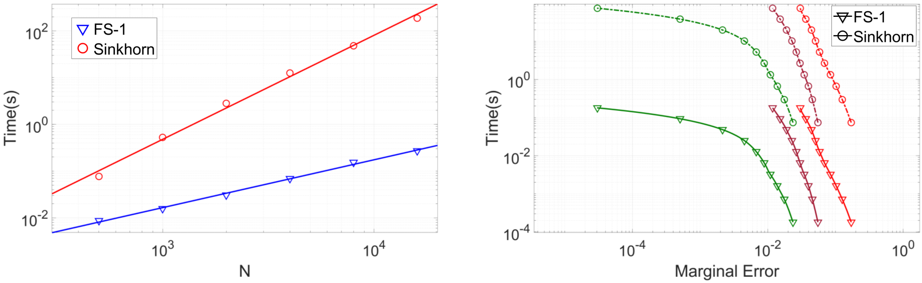
Figure 1: The 1D random distribution problem. Left: The comparison of computational time between the FS-1 algorithm and the Sinkhorn algorithm with different numbers of grid pointss $N$. Right: The computational time required to reach the corresponding marginal error under different regularization parameter $\varepsilon=0.1$(Green), $\varepsilon=0.01$(Purple), and $\varepsilon=0.001$(Red).

5.2 Ricker wavelet

Next, we consider the computation of the Wasserstein-1 metric between the Ricker wavelet

$$R(t)=A(1-2\pi^{2}f_{0}^{2}t^{2})e^{-\pi^{2}f_{0}^{2}t^{2}},$$

and its translation $R(t-s)$. The Ricker wavelet is commonly used to model source time function in seismology [8]. Here $f_{0}$ is the dominant frequency, and $A$ denotes the wave amplitude. For simplicity, we set

$$f_{0}=1,\quad A=1.$$

Since the Ricker wavelet is not always positive over the entire time duration, we will square and normalize it for the comparisons of the Wasserstein-1. In [27], a new normalization method with better convexity is given as follows:

$$D(f,g)=W_{1,\varepsilon}\left(\frac{\frac{f^{2}}{\left\|f^{2}\right\|}+\delta}{1+L\delta},\frac{\frac{g^{2}}{\left\|g^{2}\right\|}+\delta}{1+L\delta}\right),$$ (5.10)

where $\delta$ is a sufficiently small parameter to improve numerical stability, and $L$ is a given parameter to guarantee that the two functions being compared are normalized.

Below, we randomly select the translation parameter $s=-1.2032$. This parameter can ensure that the two Ricker wavelets $R(t)$ and $R(t-s)$ are sufficiently far apart. And the small parameter $\delta=10^{-3}$. We repeated the experiment 100 times, and each experiment was performed for 500 iterations. In Table 2, we output the averaged computational time of two different algorithms. We also present the computational time required to reach the corresponding marginal error under different regularization parameters $\varepsilon$ for the distribution with dimension $N=10000$, see Figure 2 (Left) for illustration, from which, we can draw the same conclusions as those in Subsection 5.1.

In Figure 2 (Right), we also discuss the impact of the log-domain stabilization technique for $\varepsilon=0.001$. Without the technique, the Sinkhorn algorithm terminates abnormally at the 97th iteration and the FS-1 algorithm terminates abnormally at the 104th iteration. By introducing the log-domain stabilization technique, neither algorithm is terminated abnormally. Moreover, the stabilized FS-1 algorithm still maintains a significant efficiency advantage over the stabilized Sinkhorn algorithm.

N	Computational time (s)		Speed-up ratio	$||P_{NB}-P||_{F}$
	FS-1	Sinkhorn
500	$4.90\times 10^{-3}$	$2.30\times 10^{-2}$	$4.69\times 10^{0}$	$5.67\times 10^{-16}$
2000	$1.52\times 10^{-2}$	$1.36\times 10^{0}$	$8.93\times 10^{1}$	$1.81\times 10^{-17}$
8000	$5.96\times 10^{-2}$	$2.81\times 10^{1}$	$4.72\times 10^{2}$	$1.22\times 10^{-16}$

Table 2: The Ricker wavelet problem. The comparison between the Sinkhorn algorithm and the FS-1 algorithm with the different number of grid points $N$. The regularization parameter $\varepsilon=0.01$. Columns 2-4 are the averaged computational time of the two algorithms and the speed-up ratio of the FS-1 algorithm. Column 5 is the Frobenius norm of the difference between the transport plan computed by the two algorithms.

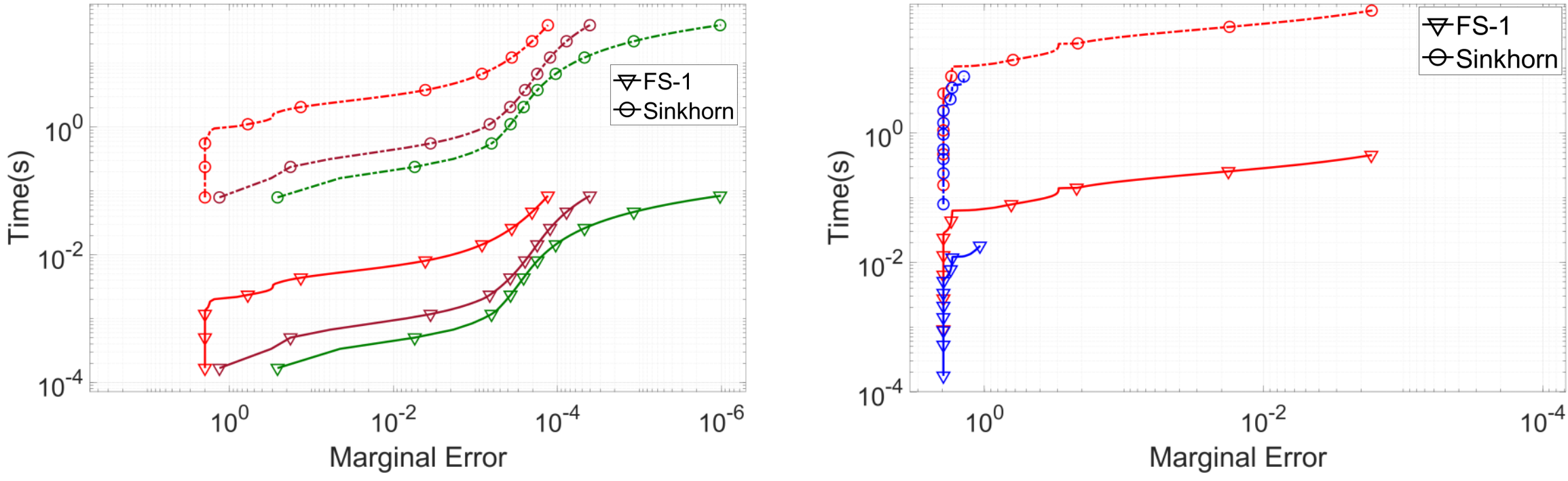
Figure 2: The Ricker wavelet problem. Left: The computational time required to reach the corresponding marginal error under different regularization parameter $\varepsilon=0.1$(Green), $\varepsilon=0.05$(Purple), and $\varepsilon=0.01$(Red). Right: The comparison between the Sinkhorn-type algorithms with (Red) and without (Blue) the log-domain stabilization for $\varepsilon=0.001$.

5.3 2D Random distributions

Next, we discuss the performance of the FS-1 algorithm in two dimension. This Subsection generalizes the 1D random distributions in Subsection 5.1 to 2D random distributions. The basic settings are almost the same as in Subsection 5.1. And we need to compute the Wasserstein-1 metric between two $N\times N$ dimensional random vectors, where $N$ is the number of grid points at each dimension. Without loss of generality, we set $h_{1}=h_{2}=1$. We also tested 100 random experiments, and each experiment was performed for 1000 iterations. The averaged computational time for different numbers of nodes $N\times N$ of the two algorithms are output in Table 3 and Figure 3 (Left). By data fitting, we can see the empirical complexity of the FS-1 algorithm is $O(N^{1.66})$ , while that of the Sinkhorn algorithm is $O(N^{4.44})$. These results are even better than the expected $O(N^{2})$ complexity for the FS-1 algorithm. This again shows the big efficiency advantage of the FS-1 algorithm compared to the Sinkhorn algorithm. In Figure 3 (Right), we also present the computational time required to reach the corresponding marginal error under different regularization parameters $\varepsilon$ for the random distribution with dimension $100\times 100$. Obviously, the FS-1 algorithm still maintains the efficiency advantage for more than two orders of magnitude.

$N\times N$	Computational time (s)		Speed-up ratio	$||P_{NB}-P||_{F}$
	FS-1	Sinkhorn
10$\times$10	$1.27\times 10^{-2}$	$8.02\times 10^{-2}$	$6.34\times 10^{0}$	$1.20\times 10^{-17}$
20$\times$20	$2.01\times 10^{-2}$	$6.73\times 10^{-1}$	$3.34\times 10^{1}$	$5.96\times 10^{-18}$
40$\times$40	$7.38\times 10^{-2}$	$1.38\times 10^{1}$	$1.87\times 10^{2}$	$3.00\times 10^{-18}$
80$\times$80	$2.64\times 10^{-1}$	$4.78\times 10^{2}$	$1.81\times 10^{3}$	$1.55\times 10^{-18}$
160$\times$160	$1.08\times 10^{0}$	$1.38\times 10^{4}$	$1.28\times 10^{4}$	$7.68\times 10^{-19}$

Table 3: The 2D random distribution problem. The comparison between the Sinkhorn algorithm and the FS-1 algorithm with the different number of grid points $N\times N$. The regularization parameter $\varepsilon=0.01$. Columns 2-4 are the averaged computational time of the two algorithms and the speed-up ratio of the FS-1 algorithm. Column 5 is the Frobenius norm of the difference between the transport plan computed by the two algorithms.

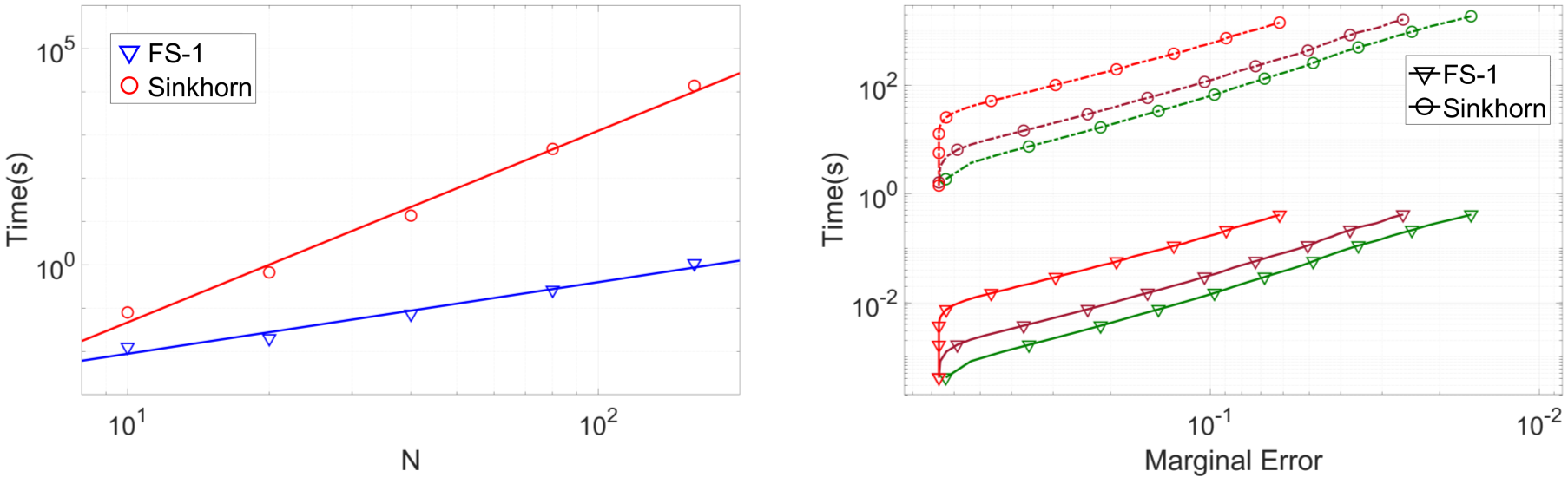
Figure 3: The 2D random distribution problem. Left: The comparison of computational time between the FS-1 algorithm and the Sinkhorn algorithm with different numbers of grid nodes $N$. Right: The computational time required to reach the corresponding marginal error under different regularization parameter $\varepsilon=0.1$(Green), $\varepsilon=0.05$(Purple), and $\varepsilon=0.01$(Red).

5.4 Image matching problem

An important application of the optimal transport in 2D is to match images. OT plays a fundamental role of related tasks including density regularization [6], image registration [18], and optical flow [10]. The complexity advantage of the FS-1 algorithm compared to the Sinkhorn algorithm can further enable practical applications of optimal transport in high-resolution images.

Here we consider the image matching experiment. We randomly select two images, see Figure 4 for illustration, from the DIV2K dataset[1], where the images have 2K pixels for at least one of the axes (vertical or horizontal). Considering that the resolutions of the images are different, we first sample them to the same scale $N\times N$. Without loss of generality, we set $h_{1}=h_{2}=1$. In addition, to facilitate the optimal transport comparison, we convert them to grayscale images and normalize them using formula (5.10) with $\delta=10^{-7}$. Again, we repeated the experiment $100$ times and each experiment was performed for $1000$ iterations.

Figure 4: The image matching problem. Illustration of images.

In Table 4, we output the averaged computational time of two different algorithms. It should be emphasized that the computational time of the Sinkhorn algorithm is too long for large-scale images, so there is no result. However, the FS-1 algorithm can still handle this simply. We also present the computational time required to reach the corresponding marginal error under different regularization parameters $\varepsilon$. Here, the image size is $100\times 100$, see Figure 5 (Left) for illustration, from which we can draw the same conclusions as those in Subsection 5.3.

In Figure 5 (Right), we also discuss the impact of the log-domain stabilization technique for $\varepsilon=0.01$. Without the technique, the Sinkhorn algorithm and the FS-1 algorithm both terminate abnormally at the 138th iteration. By introducing the log-domain stabilization technique, neither algorithm is terminated abnormally. Moreover, the stabilized FS-1 algorithm still maintains a significant efficiency advantage over the stabilized Sinkhorn algorithm.

$N\times N$	Computational time (s)		Speed-up ratio	$\left\|P_{NB}-P\right\|_{F}$
	FS-1	Sinkhorn
100$\times$100	$4.10\times 10^{-1}$	$1.32\times 10^{3}$	$3.23\times 10^{3}$	$2.28\times 10^{-17}$
200$\times$200	$1.72\times 10^{0}$	$3.08\times 10^{4}$	$1.79\times 10^{5}$	$9.52\times 10^{-18}$
400$\times$400	$7.23\times 10^{0}$	$-$	$-$	$-$
800$\times$800	$3.20\times 10^{1}$	$-$	$-$	$-$

Table 4: The image matching problem. The comparison between the Sinkhorn algorithm and the FS-1 algorithm with the different total number of grid nodes $N\times N$. The regularization parameter $\varepsilon=1$. Columns 2-4 are the averaged computational time of the two algorithms and the speed-up ratio of the FS-1 algorithm. Column 5 is the Frobenius norm of the difference between the transport plan computed by the two algorithms.

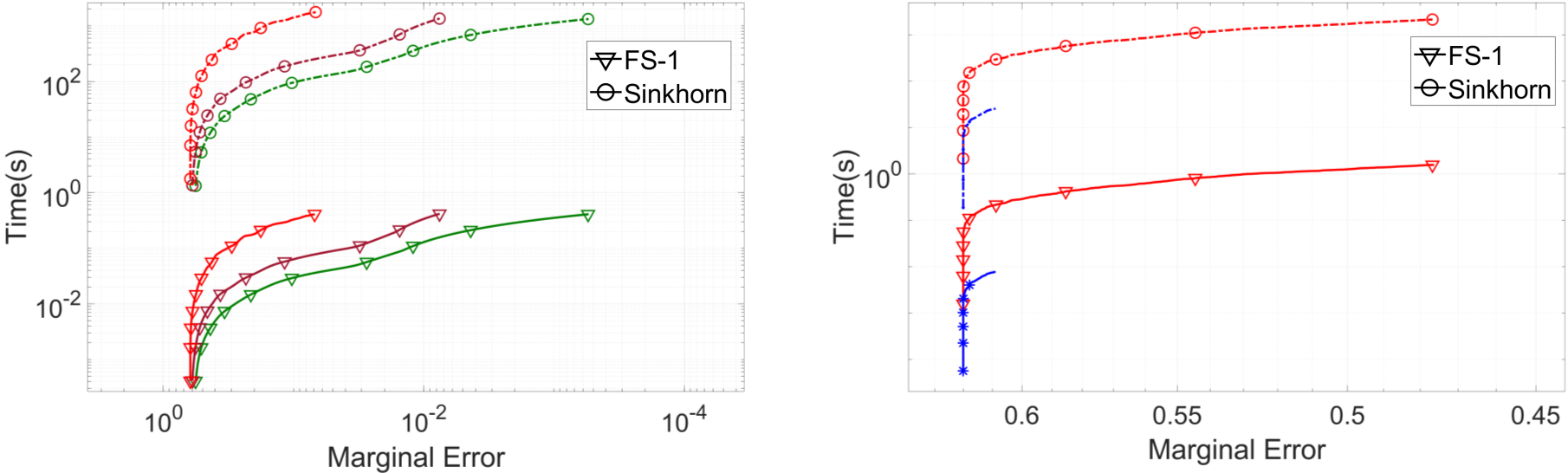
Figure 5: The image matching problem. Left: The computational time required to reach the corresponding marginal error under different regularization parameter $\varepsilon=1$(Green), $\varepsilon=0.5$(Purple), and $\varepsilon=0.1$(Red). Right: The comparison between the Sinkhorn-type algorithms with (Red) and without (Blue) the log-domain stabilization for $\varepsilon=0.01$.

6 Conclusion

In this paper, we propose an efficient (abbreviated as FS-1) algorithm to compute the Wasserstein-1 metric with linear computational cost per iteration. This method is developed by discovering the natural structure of Sinkhorn’s kernel, which allows a matrix-vector multiplication to be carried out exactly with $O(n)$ cost for each iteration by using Qin Jiushao’s or Horner’s method for efficient polynomial evaluation. Moreover, the FS-1 algorithm can also be adapted to the widely used log-domain stabilization technique. As shown by numerous experiments, the FS-1 algorithm achieves a huge speed advantage without losing accuracy.

Finally, this paper mainly considers the acceleration of the Sinkhorn algorithm in the matrix-vector multiplication. It is well known that the number of iterations of the Sinkhorn algorithm will significantly increase with the increase of numerical accuracy, which leads to slow convergence. In [49], the Inexact Proximal point method for the Optimal Transport problem (IPOT) was proposed for this problem. We believe that FS-1 and IPOT can be effectively combined to develop a new algorithm for solving the Optimal Transport problem with fast convergence and low complexity. We are currently investigating this important extension and hope to report the progress in a future paper.

References

- [1] E. Agustsson and R. Timofte, Ntire 2017 challenge on single image super-resolution: Dataset and study, in The IEEE Conference on Computer Vision and Pattern Recognition (CVPR) Workshops, July 2017.
- [2] J. Altschuler, F. Bach, A. Rudi, and J. Weed, Massively scalable Sinkhorn distances via the Nyström method, Advances in Neural Information Processing Systems, 1050 (2018), p. 12.
- [3] J. Altschuler, J. Weed, and P. Rigollet, Near-linear time approximation algorithms for optimal transport via Sinkhorn iteration, arXiv preprint arXiv:1705.09634, (2017).
- [4] J.-D. Benamou and Y. Brenier, A computational fluid mechanics solution to the Monge-Kantorovich mass transfer problem, Numerische Mathematik, 84 (2000), pp. 375–393.
- [5] J.-D. Benamou, B. D. Froese, and A. M. Oberman, Numerical solution of the optimal transportation problem using the Monge–Ampère equation, Journal of Computational Physics, 260 (2014), pp. 107–126.
- [6] M. Burger, M. Franek, and C.-B. Schönlieb, Regularized regression and density estimation based on optimal transport, Applied Mathematics Research eXpress, 2012 (2012), pp. 209–253.
- [7] G. Buttazzo, L. De Pascale, and P. Gori-Giorgi, Optimal-transport formulation of electronic density-functional theory, Physical Review A, 85 (2012), p. 062502.
- [8] J. Chen, Y. Chen, H. Wu, and D. Yang, The quadratic Wasserstein metric for earthquake location, Journal of Computational Physics, 373 (2018), pp. 188–209.
- [9] L. Chizat, G. Peyré, B. Schmitzer, and F.-X. Vialard, Scaling algorithms for unbalanced optimal transport problems, Mathematics of Computation, 87 (2018), pp. 2563–2609.
- [10] P. Clarysse, B. Delhay, M. Picq, and J. Pousin, Optimal extended optical flow subject to a statistical constraint, Journal of Computational and Applied Mathematics, 234 (2010), pp. 1291–1302.
- [11] P. L. Combettes and J.-C. Pesquet, Proximal splitting methods in signal processing, in Fixed-Point Algorithms for Inverse Problems in Science and Engineering, Springer, 2011, pp. 185–212.
- [12] C. Cotar, G. Friesecke, and C. Klüppelberg, Density functional theory and optimal transportation with Coulomb cost, Communications on Pure and Applied Mathematics, 66 (2013), pp. 548–599.
- [13] M. Cuturi, Sinkhorn distances: Lightspeed computation of optimal transport, Advances in Neural Information Processing Systems, 26 (2013), pp. 2292–2300.
- [14] B. Engquist, K. Ren, and Y. Yang, The quadratic Wasserstein metric for inverse data matching, Inverse Problems, 36 (2020), p. 055001.
- [15] B. D. Froese, Numerical methods for the elliptic Monge-Ampere equation and optimal transport, PhD thesis, Science: Department of Mathematics, 2012.
- [16] B. D. Froese and A. M. Oberman, Convergent finite difference solvers for viscosity solutions of the elliptic Monge–Ampère equation in dimensions two and higher, SIAM Journal on Numerical Analysis, 49 (2011), pp. 1692–1714.
- [17] I. Goodfellow, J. Pouget-Abadie, M. Mirza, B. Xu, D. Warde-Farley, S. Ozair, A. Courville, and Y. Bengio, Generative adversarial nets, Advances in Neural Information Processing Systems, 27 (2014).
- [18] S. Haker, L. Zhu, A. Tannenbaum, and S. Angenent, Optimal mass transport for registration and warping, International Journal of Computer Vision, 60 (2004), pp. 225–240.
- [19] H. Heaton, S. W. Fung, A. T. Lin, S. Osher, and W. Yin, Wasserstein-based projections with applications to inverse problems, arXiv preprint arXiv:2008.02200, (2020).
- [20] W. G. Horner, Xxi. a new method of solving numerical equations of all orders, by continuous approximation, Philosophical Transactions of the Royal Society of London, (1819), pp. 308–335.
- [21] Y. Hu, H. Chen, and X. Liu, A global optimization approach for multi-marginal optimal transport problems with Coulomb cost, arXiv preprint arXiv:2110.07352, (2021).
- [22] J. Kleinberg and E. Tardos, Algorithm design, Pearson Education India, 2006.
- [23] J. Klicpera, M. Lienen, and S. Günnemann, Scalable optimal transport in high dimensions for graph distances, embedding alignment, and more, in International Conference on Machine Learning, PMLR, 2021, pp. 5616–5627.
- [24] T. Le, M. Yamada, K. Fukumizu, and M. Cuturi, Tree-sliced variants of Wasserstein distances, Advances in Neural Information Processing Systems, 32 (2019), pp. 12304–12315.
- [25] W. Li, E. K. Ryu, S. Osher, W. Yin, and W. Gangbo, A parallel method for earth mover’s distance, Journal of Scientific Computing, 75 (2018), pp. 182–197.
- [26] X. Li, D. Sun, and K.-C. Toh, An asymptotically superlinearly convergent semismooth Newton augmented Lagrangian method for linear programming, SIAM Journal on Optimization, 30 (2020), pp. 2410–2440.
- [27] Z. Li, Y. Tang, J. Chen, and H. Wu, The quadratic Wasserstein metric with squaring scaling for seismic velocity inversion, arXiv preprint arXiv:2201.11305, (2022).
- [28] A. T. Lin, W. Li, S. Osher, and G. Montúfar, Wasserstein proximal of GANs, in International Conference on Geometric Science of Information, Springer, 2021, pp. 524–533.
- [29] T. Lin, N. Ho, and M. I. Jordan, On the efficiency of the Sinkhorn and Greenkhorn algorithms and their acceleration for optimal transport, International Conference on Machine Learning, (2019).
- [30] J. Liu, W. Yin, W. Li, and Y. T. Chow, Multilevel optimal transport: a fast approximation of Wasserstein-1 distances, SIAM Journal on Scientific Computing, 43 (2021), pp. A193–A220.
- [31] C. Meng, Y. Ke, J. Zhang, M. Zhang, W. Zhong, and P. Ma, Large-scale optimal transport map estimation using projection pursuit, Advances in Neural Information Processing Systems, 32 (2019), pp. 8118–8129.
- [32] C. Meng, J. Yu, J. Zhang, P. Ma, and W. Zhong, Sufficient dimension reduction for classification using principal optimal transport direction, Advances in Neural Information Processing Systems, 33 (2020).
- [33] L. Métivier, R. Brossier, Q. Mérigot, E. Oudet, and J. Virieux, Measuring the misfit between seismograms using an optimal transport distance: Application to full waveform inversion, Geophysical Supplements to the Monthly Notices of the Royal Astronomical Society, 205 (2016), pp. 345–377.
- [34] L. Métivier, R. Brossier, Q. Merigot, É. Oudet, and J. Virieux, An optimal transport approach for seismic tomography: Application to 3D full waveform inversion, Inverse Problems, 32 (2016), p. 115008.
- [35] J. Needham, Science and civilisation in China, vol. 5, Cambridge University Press, 1974.
- [36] O. Pele and M. Werman, Fast and robust earth mover’s distances, in 2009 IEEE 12th International Conference on Computer Vision, IEEE, 2009, pp. 460–467.
- [37] G. Peyré, M. Cuturi, et al., Computational optimal transport: With applications to data science, Foundations and Trends® in Machine Learning, 11 (2019), pp. 355–607.
- [38] Y. Rubner, C. Tomasi, and L. J. Guibas, The earth mover’s distance as a metric for image retrieval, International Journal of Computer Vision, 40 (2000), pp. 99–121.
- [39] O. Russakovsky, J. Deng, H. Su, J. Krause, S. Satheesh, S. Ma, Z. Huang, A. Karpathy, A. Khosla, M. Bernstein, A. C. Berg, and L. Fei-Fei, ImageNet Large Scale Visual Recognition Challenge, International Journal of Computer Vision (IJCV), 115 (2015), pp. 211–252.
- [40] E. K. Ryu, Y. Chen, W. Li, and S. Osher, Vector and matrix optimal mass transport: theory, algorithm, and applications, SIAM Journal on Scientific Computing, 40 (2018), pp. A3675–A3698.
- [41] E. K. Ryu, W. Li, P. Yin, and S. Osher, Unbalanced and partial L1 Monge–Kantorovich problem: A scalable parallel first-order method, Journal of Scientific Computing, 75 (2018), pp. 1596–1613.
- [42] F. Santambrogio, Optimal transport for applied mathematicians, Birkäuser, NY, 55 (2015), p. 94.
- [43] M. Scetbon and M. Cuturi, Linear time Sinkhorn divergences using positive features, Advances in Neural Information Processing Systems, (2020).
- [44] M. Scetbon, M. Cuturi, and G. Peyré, Low-rank Sinkhorn factorization, International Conference on Machine Learning, (2021).
- [45] R. Sinkhorn, Diagonal equivalence to matrices with prescribed row and column sums, The American Mathematical Monthly, 74 (1967), pp. 402–405.
- [46] J. Solomon, F. De Goes, G. Peyré, M. Cuturi, A. Butscher, A. Nguyen, T. Du, and L. Guibas, Convolutional wasserstein distances: Efficient optimal transportation on geometric domains, ACM Transactions on Graphics (ToG), 34 (2015), pp. 1–11.
- [47] Y. Takezawa, R. Sato, and M. Yamada, Supervised tree-Wasserstein distance, in Proceedings of the 38th International Conference on Machine Learning, M. Meila and T. Zhang, eds., vol. 139 of Proceedings of Machine Learning Research, PMLR, 18–24 Jul 2021, pp. 10086–10095.
- [48] C. Villani, Optimal transport: old and new, vol. 338, Springer, 2009.
- [49] Y. Xie, X. Wang, R. Wang, and H. Zha, A fast proximal point method for computing exact wasserstein distance, in Uncertainty in artificial intelligence, PMLR, 2020, pp. 433–453.
- [50] L. Yang, J. Li, D. Sun, and K.-C. Toh, A fast globally linearly convergent algorithm for the computation of Wasserstein barycenters., Journal of Machine Learning Research, 22 (2021), pp. 1–37.
- [51] Y. Yang, B. Engquist, J. Sun, and B. F. Hamfeldt, Application of optimal transport and the quadratic Wasserstein metric to full-waveform inversion, Geophysics, 83 (2018), pp. R43–R62.